Advances in surface water and ocean topography for fine-scale eddy identification from altimeter sea surface height merging maps in the South China Sea

The recently launched Surface Water and Ocean Topography (SWOT) satellite mission has reduced the noise levels and increased resolution, thereby improving the ability to detect previously unobserved fine-scale signals. We employed a method to utilize the unique and advanced abilities of SWOT to validate the accuracy of identified eddies in merged maps of a widely used Archiving, Validation, and Interpretation of Satellite Oceanographic (AVISO) data product and a newly implemented two-dimensional variational method (2DVAR), which uses a $\mathrm{1}/\mathrm{12}$° grid and reduces decorrelation of spatial length scales. SWOT data are more likely to provide detailed comparisons of eddy boundaries for fine-scale to mesoscale structures compared with conventional in situ data (e.g., drifting buoys). The validation results demonstrate that, compared with AVISO, the 2DVAR method exhibited greater consistency with the SWOT observations, especially at small scales, confirming the accuracy and ability of the 2DVAR method in the reconstruction and resolution of fine-scale oceanic dynamical structures.

1 Introduction

The ocean has diverse spatial length scales of dynamical processes, from mesoscale signals at approximately 100–1000 km to submesoscale processes below 100 km. Fine-scale ocean processes are characterized by a spatial variability of 1–100 km and a temporal variability of days to months (Lévy et al., 2024). These processes are primarily revealed through the absolute dynamic topography (ADT), which is an estimate of sea surface height (SSH) above the geoid. The ADT also plays a substantial role in the thermohaline circulation, atmosphere–ocean interactions, physical–biological–biochemical interactions, and numerical modeling of coupled atmospheric–oceanic systems (Chelton et al., 2007; Ma et al., 2016; Mahadevan, 2016; Wunsch and Heimbach, 2013).

Global satellite altimeters offer systematic ADT measurements and mapping of ocean topography, currently providing the most effective data for detecting and tracking large and mesoscale ocean dynamic signals (Chelton et al., 2007; Mason et al., 2014; Zhang et al., 2023). Due to differences in orbit cycles and swaths from different satellites, the observing data exhibit misalignment in both space and time. Consequently, ensemble Kalman filtering or data assimilation techniques based on optimal estimation methods are employed to merge data from different satellites, yielding a spatiotemporally continuous ADT map (Cohn, 1997; Le Traon et al., 1998; Taburet et al., 2019). The main techniques of data assimilation typically include the homogenization and cross-calibration of multisource altimetry data, continuous calibration of reference orbits, cross-calibration between altimeters, long-wavelength error correction, and error budget modeling. Finally, optimal interpolation is used for gridding to generate daily gridded products and derived products (Pujol et al., 2016). Diverse merging methods result in disparate capacities for capturing oceanic dynamic signals, which can be assessed by metrics such as effective resolution and eddy kinetic energy (Ballarotta et al., 2019, 2020; Pascual et al., 2007; Taburet et al., 2019; Wang et al., 2021). Those assessment methods that rely on conventional measurement data are inherently limited by linear and long temporal sampling, low resolution, and other observational uncertainties, making them unsuitable for assessing merged maps in regions characterized by intricate multiscale oceanic dynamic signals.

The Surface Water and Ocean Topography (SWOT) satellite, launched in December 2022, comprises a new generation of Ka-band radar interferometers (KaRIns), which reduces instrument noise by 2 orders of magnitude compared to that of the conventional satellites (Abdalla et al., 2021; Fu et al., 2024). The KaRIn technique allows mapping of two-dimensional ADT with a 120 km swath, which is over 5 times the width of a conventional nadir, and offers an unprecedented 15 km spatial resolution for an altimeter satellite (Dufau et al., 2016; Morrow et al., 2019; Wang and Fu, 2019). Globally, SWOT data have undergone in situ observational calibration and validation and data assimilation application studies before their formal use for global mapping, confirming the capability of detecting previously unobserved fine-scale signals, reinforcing the capabilities of ocean monitoring and signifying a pivotal advancement in enhancing spatial resolution (Martin et al., 2024; Ubelmann et al., 2024; Verger-Miralles et al., 2024; Zhang et al., 2024). However, the intrinsic challenge posed by the discrepancy between low temporal and high spatial resolutions requires further interpretation before direct utilization as inputs for ADT merged maps in future research endeavors.

This study aims to validate the accuracy and reliability of different merging methods, specifically two-dimensional variation (2DVAR) and the Archiving, Validation, and Interpretation of Satellite Oceanographic (AVISO) data product, in reconstructing oceanic dynamic signals, with a particular focus on fine-scale eddies. It introduces a novel application scenario and methodology for utilizing state-of-the-art international sea surface observation data. Furthermore, it offers a new framework for assessing the quality of merged maps, which can provide valuable insights and guidance for the development of future merging techniques.

2 Materials and methods

2.1 ADT merging maps

The SWOT mission consists of two phases: the science phase, which conducted 21 d repeat sampling from 7 September to 21 November 2023, and the calibration and validation phase (CALVAL), which performed 1 d rapid sampling from 1 April to 31 July 2023 (AVISO/DUACS, 2024). The CALVAL phase data were used exclusively in the second part of Sect. 3.2 to analyze the temporal evolution of eddies. In contrast, the science phase data were the primary datasets for examining the spatial dynamic structures and performing statistical analyses of eddy characteristics. Although the CALVAL phase sampled a limited sea surface area due to its fixed rapid-sampling orbit, this orbit covered part of the South China Sea (SCS) and facilitated the capture of time-evolving fine-scale eddy structures in the SCS. The nadir observation points, located between two slices of KaRIn observations (Fig. 1a), were excluded in both phases due to their high error rates and our focus on the advanced KaRIn technology. To ensure consistency in data resolution and to focus the current study on the fine scale to the mesoscale, we employed a regional averaging method to reduce the resolution of the SWOT data from the original 2 km sampling interval to $\mathrm{1}/\mathrm{12}$°. Owing to the inclination angle between the SWOT satellite orbital plane and the equatorial plane, each downsampled square region is covered by observations. Consequently, interpolation across swath gaps is unnecessary, thereby avoiding the substantial errors associated with interpolating these gaps.

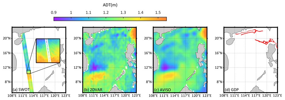
Figure 1 Four datasets of absolute dynamic topography (ADT) in the South China Sea. (a) SWOT, (b) 2DVAR, (c) AVISO, and (d) GDP. The ADT data in panels (a), (b), and (c) were obtained on 12 September 2023, and panel (d) covers the entire period of the science phase.

We employed two types of ADT merged data to generate corresponding eddy identification ensembles. The first ADT product (Fig. 1b) was produced using a ±11 d time window near-real-time (NRT) two-dimensional variation (2DVAR) method with a $\mathrm{1}/\mathrm{12}$° grid resolution. It employs optimized background and observation errors to decorrelate the length scales in the merging process with an improved method for calculating the background error covariance matrix (Liu et al., 2020). The second ADT merged map (Fig. 1c) was a product released by AVISO, which uses the optimal interpolation method (Pujol et al., 2016) with a global $\mathrm{1}/\mathrm{4}$° grid resolution. During the science phase of the SWOT mission, the AVISO merged-map delayed-time (DT) products utilized SWOT nadir data as an input source (Copernicus Marine Service repository, 2023b). To maintain the independence of the datasets, we employed NRT products, which do not include SWOT nadir data (Copernicus Marine Service repository, 2023a). Similarly, during the CALVAL phase of the SWOT mission, we used an older version of the DT products, which do not include SWOT data as an input source. The DT products are reanalysis datasets that incorporate the highest-quality altimeter measurements and geophysical corrections to minimize the risk of mass loss or false signals over time. The NRT data provide ready-to-use, real-time published altimeter data from all available missions. In the data processing, the DT products are computed optimally using a centered computation time window of ±6 weeks around the date of the map to be computed. In the NRT processing, future data are not available; therefore, the computation time window covers the period from 7 weeks prior to the computation date. Both the AVISO and 2DVAR methods were based on the principle of optimal estimation and were calculated using all available on-orbit altimeter mission data, including Jason-3, Sentinel-3A, HY-2B, Saral/AltiKa, CryoSat-2, Sentinel-3B, and Sentinel-6A. Notably, the 2DVAR method successfully reduced the effective resolution to approximately half that of AVISO, enhancing the resolution of signals from fine-scale to mesoscale eddies, particularly in areas with rich eddy kinetic energy, such as the SCS and the northwestern Pacific Ocean (Jiang et al., 2022; Liu et al., 2023).

The SCS is a significant dynamic marginal sea in the northwestern Pacific, featuring complex bathymetry, a large area, and multiple straits that facilitate water exchange with the Pacific and Indian oceans (Chen et al., 2023). It serves as an exemplary model of an open ocean with well-defined continental shelves, shelf breaks, and a central deep basin. In the SCS, the first obliquely pressured Rossby deformation radius was less than 20 km in winter (Cai et al., 2008), suggesting a rich environment for fine-scale oceanic dynamical processes. Additionally, the SCS receives energy transport from the submesoscale energy reservoir of the Kuroshio via the western boundary currents, resulting in a dense concentration of mesoscale and fine-scale processes on the 10 km scale (Lin et al., 2020; Ni et al., 2021; Zu et al., 2019). Thus, this study of the SCS holds substantial significance and a reference value for understanding complex dynamic marginal seas and the broader northwestern Pacific region.

2.2 Eddy identification

Currently, the main methods for eddy identification based on satellite altimeters include the Okubo–Weiss (OW) parameter from the velocity field method, the curvature center method, the surrounding angle method, the local extreme of sea surface topography method, the local and normalized angular momentum method, and the Lagrangian coherent structure (LCS) method (Chelton et al., 2011; Laxenaire et al., 2018; Mcwilliams, 1990; Mkhinini et al., 2014; Okubo, 1970; Sadarjoen and Post, 2000; Weiss, 1991). Of these, the sea surface topography method provides the clearest and most cohesive identification of eddies, regardless of their size or boundary (Chen et al., 2021). Therefore, this research employed a sea surface topography method based on contour analysis for eddy identification in 2DVAR and AVISO ADT merged maps as well as in SWOT maps during both phases of the SWOT mission (Chelton et al., 2011). The eddy tracking was only adopted during the science phase because of the fixed observation area of the CALVAL phase. It is worth noting that, due to SWOT observation data limitations, we are currently unable to identify eddies located at the edges of the swath or outside the swath. To avoid the influence of grid resolution, different merged maps were interpolated to a high-resolution grid with the same resolution ($\mathrm{1}/\mathrm{12}$°). The outermost circle of the closed contours with a 1 mm step in the ADT difference containing the unique center was recognized as the “quasi-eddy edge”, and a minimum of only three points were retained. Each quasi-eddy edge was then contracted inward until it corresponded to a single center. Lastly, the geometric center of the innermost circle of the closed contours was identified as the eddy center. This process allowed the determination of the eddy boundary, type, radius, and amplitude. All possible eddies with a difference in ADT between the eddy center and the boundary contour line of less than ±2 cm were excluded from further analysis.

2.3 Eddy validation

The accuracy and reliability of the identified eddies were validated and assessed using two observational ADT datasets as true values. First, the Level-3 LR ADT v1.0.2 datasets from the SWOT product were used for eddy validation, and a visualization method was employed to examine the clarity and intuitiveness of the eddy boundaries. The Level-3 data are more suitable for capturing fine-scale to mesoscale structures compared to the Level-4 products, which rely on merging methods and data from other satellites (Ballarotta et al., 2023). The 2 km sampling interval allowed the SWOT data to capture finer-scale signals that are not the primary focus of the current research. Therefore, spatial average filtering with a $\mathrm{1}/\mathrm{12}$° grid was conducted to filter out those finer-scale signals (Fig. 1a), highlighting the fine-scale to mesoscale eddies in this study.

Before the validation process, all identified eddies were preliminarily evaluated to ensure that they could be matched with a specific SWOT eddy. Once a successful match was established, the eddy reconstruction of the ADT map was considered correct and retained along with its corresponding eddy captured from the SWOT map. Only eddies that met the following three criteria were considered to match the SWOT eddy, which was assumed to be topical:

1. The rotation directions or types of the merged-map eddy and the SWOT eddy are the same.

2. The distance between the center of the merged-map eddy and the SWOT eddy is less than 50 km.

3. The difference in radius between the merged-map eddy and the SWOT eddy is less than 120 km.

The criteria were set according to the KaRIn swath, which is approximately 120 km for the full swath and approximately 50 km for the half swath. After filtering out eddies that cannot be matched with SWOT, a systematic standardization process was adopted to make merged-map eddies comparable with SWOT eddies in terms of spatial scales and relative locations (Chen and Yu, 2024). The operation aims to standardize SWOT eddies of diverse sizes and proportionally scale the eddies in the 2DVAR and AVISO merged maps relative to those in SWOT, thereby retaining the relative differences between the merged maps and SWOT. The normalization and proportional scaling allow statistical synthesis of differences between thousands of eddies into a single standard grid composite map, effectively characterizing the radius discrepancies between the merged maps and the SWOT eddies. Firstly, the scale normalization factor α was calculated for each SWOT eddy to adjust it to a fixed size based on the eddy radius:

$$\begin{array}{}\text{(1)}& {\mathit{\alpha }}_i={\displaystyle \frac{\frac{\mathrm{1}}{N}\sum _{i=\mathrm{1}}^n{r}_i}{r{}_i}},\end{array}$$

where i is the index of the ith eddy in the SWOT ensemble, N denotes the total number of eddies, and r represents the radius of the eddy. To eliminate the absolute positional differences, we established a local coordinate system with the center of the normalized SWOT eddy as the origin. The geographical coordinates of the ith SWOT eddy center (X_i,S, Y_i,S) were subtracted from those of the corresponding merged-map eddy centers (X_i,c, Y_i,c) and boundary points (X_i,bm, Y_i,bm).

$$\begin{array}{}\text{(2)}& \left\{\begin{array}{l}\left(X_{i,\mathrm{c}}^{\prime },Y_{i,\mathrm{c}}^{\prime }\right)=\left(X_{i,\mathrm{c}}-X_{i,\mathrm{S}},Y_{i,\mathrm{c}}-Y_{i,\mathrm{S}}\right)\\ \left(X_{i,\mathrm{bm}}^{\prime },Y_{i,\mathrm{bm}}^{\prime }\right)=\left(X_{i,\mathrm{bm}}-X_{i,\mathrm{S}},Y_{i,\mathrm{bm}}-Y_{i,\mathrm{S}}\right)\end{array}\right.\end{array}$$

The new center and boundary points of the ith merged-map eddy in the local coordinate system are ($X_{i,\mathrm{c}}^{\prime }$,$Y_{i,\mathrm{c}}^{\prime })$ and ($X_{i,\mathrm{bm}}^{\prime },Y_{i,\mathrm{bm}}^{\prime })$, where bm denotes the index of the boundary point.

Based on the coordinate system transformation, the position information of the merged-map eddies in the new coordinate system was scaled using the SWOT eddy normalization factor α. Considering that eddy scaling is related to radial distance, this step applied a polar coordinate transformation to extract the radial distances r_i,c,r_i,bm and angles θ_i,c, θ_i,bm of the points.

$$\begin{array}{}\text{(3)}& \left\{\begin{array}{l}{r}_{i,\mathrm{c}}=\sqrt{{\left(X_{i,\mathrm{c}}^{\prime }\right)}^{\mathrm{2}}+{\left(Y_{i,\mathrm{c}}^{\prime }\right)}^{\mathrm{2}}}\\ {\mathit{\theta }}_{i,\mathrm{c}}=\arctan \left(\frac{Y_{i,\mathrm{c}}^{\prime }}{X_{i,\mathrm{c}}^{\prime }}\right)\\ r_{i,\mathrm{bm}}=\sqrt{{\left(X_{i,\mathrm{bm}}^{\prime }\right)}^{\mathrm{2}}+{\left(Y_{i,\mathrm{bm}}^{\prime }\right)}^{\mathrm{2}}}\\ {\mathit{\theta }}_{i,\mathrm{bm}}=\arctan \left(\frac{Y_{i,\mathrm{bm}}^{\prime }}{X_{i,\mathrm{bm}}^{\prime }}\right)\end{array}\right.\end{array}$$

By multiplying the coordinates by the normalization factor α, we implemented the scaling. The scaled coordinates were then transformed back to obtain geometrically similar coordinates ($X_{i,\mathrm{c}}^{\prime \prime }$, $Y_{i,\mathrm{c}}^{\prime \prime })$ and ($X_{i,\mathrm{bm}}^{\prime \prime }$, $Y_{i,\mathrm{bm}}^{\prime \prime })$.

$$\begin{array}{}\text{(4)}& \left\{\begin{array}{l}{X}_{i,\mathrm{c}}^{\prime \prime }=r_{i,\mathrm{c}}\cdot {\mathit{\alpha }}_i\cdot \cos \left({\mathit{\theta }}_{i,\mathrm{c}}\right)\\ Y_{i,\mathrm{c}}^{\prime \prime }=r_{i,\mathrm{c}}\cdot {\mathit{\alpha }}_i\cdot \sin \left({\mathit{\theta }}_{i,\mathrm{c}}\right)\\ X_{i,\mathrm{bm}}^{\prime \prime }=r_{i,\mathrm{bm}}\cdot {\mathit{\alpha }}_i\cdot \cos \left({\mathit{\theta }}_{i,\mathrm{c}}\right)\\ Y_{i,\mathrm{bm}}^{\prime \prime }=r_{i,\mathrm{bm}}\cdot {\mathit{\alpha }}_i\cdot \sin \left({\mathit{\theta }}_{i,\mathrm{bm}}\right)\end{array}\right.\end{array}$$

For comparison with SWOT, this section also describes the validation of eddies using traditional in situ drifter observations. The Global Drifter Program (GDP) data provide the positions of a 15 m depth drogue drifter at 1 h frequency and have frequently been employed in the validation and assessment of surface dynamic signals (Zhang and Qiu, 2018). These data enable studies of fine-scale to mesoscale dynamical structures and comparative evaluation of global ocean numerical models and provide input data for forecasting (Lumpkin and Elipot, 2010; Yu et al., 2019). Due to its Lagrangian nature, the drifter is more likely to respond to low pressure and high velocity in the central region of the eddy, and it then becomes entrained within the eddy as it rotates towards the center (Ohlmann et al., 2017). Thus, the trajectory of the drifter allows for the observation and capture of fine-scale and mesoscale eddies in this research. The region of interest in this study is situated within the convergence zone of the subtropical circulation, and it contains several drifter sampling areas and involves a long drift time. However, the GDP datasets are only available during the scientific phase of the SWOT mission (Fig. 1d).

3 Results

3.1 Accuracy and reliability of identified eddies

In this section, composite maps of normalized eddy ensembles for 2DVAR and AVISO ADT merged maps will be presented first, followed by a summary of the errors and characteristics of the identified eddies.

The colored areas in Fig. 2 represent the distributions of the normalized radii of eddies identified by 2DVAR and AVISO, which were successfully matched with SWOT eddies. All identified eddies were categorized into three groups based on the radii of SWOT eddies: those with radii below 10 km, between 10 and 20 km, and exceeding 20 km were classified as fine-scale (Fig. 2a), submesoscale (Fig. 2b), and mesoscale (Fig. 2c) eddies, respectively. The dashed circle lines in each component represent the normalized SWOT eddies, and the size of the colored area outside these dashed circles illustrates the discrepancy between the merged-map eddies and SWOT eddies. A grid space extent equal to twice the normalized SWOT eddy radius was chosen.

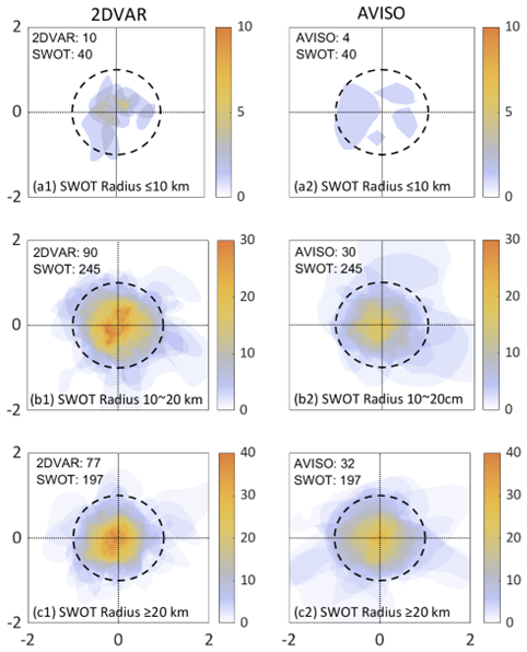
Figure 2 Composite maps of the normalized eddy identified from 2DVAR (a1, b2, c1) and AVISO (a2, b2, c2) merged maps; the color on the grid points shows the density of covered eddies, and the higher the density of the grid points, the darker the orange. The dashed circles mark the normalized SWOT eddies with radii of less than 10 km (a), 10 to 20 km (b), and more than 20 km (c). The total numbers of eddies detected by each map are in the upper-left corner.

Despite geographical and radius distribution discrepancies, the merged map shows a certain degree of accuracy and similarity to SWOT in Fig. 2. As the eddy scale increases from Fig. 2a to c, the maxima on the eddy composite maps are situated closer to the origin, and the error proportions beyond the dashed circles decrease. This suggests that the merged map is more accurate at reconstructing mesoscale eddies compared to fine-scale eddies.

To reconstruct the same SWOT eddy categories, the two merged maps exhibit different performances. Since the same color bar is applied to the eddy ensembles of the two merged maps for the same scale range, the distribution and concentration of the eddies can be judged by the intensity of the colors. It is evident that the area of the colored region outside the normalized SWOT eddies (marked by black dashed circles) on the 2DVAR merged map is smaller, especially in Fig. 2b and c. Meanwhile, despite the number of eddies identified by 2DVAR being 2 to 3 times that of AVISO, the color outside the normalized eddy circles remains a light shade of purple (i.e., no more than 10 eddies). These results suggest that the concentration of 2DVAR eddies within the normalized SWOT eddies is higher, and the eddy boundaries maintain a higher degree of consistency. Additionally, 2DVAR results in more matches with SWOT across all of the categories, particularly for SWOT eddies with scales of less than 10 km (Fig. 2a), where the number of matches is 3 times greater than that achieved by AVISO.

For all of the matched eddies, the average radii of the matched SWOT, 2DVAR, and AVISO eddies are approximately 20, 40, and 65 km, respectively, indicating a significant difference between the merged maps. The size range for all of the matched 2DVAR eddies, from 15 to 100 km, is closer to that of SWOT (ranging roughly from 8 to 54 km) than the broader span of 15 to 134 km for AVISO. Compared to the normalized eddies from AVISO, those of 2DVAR are more concentrated, and their boundaries are more precise relative to the dashed circle representing the actual SWOT eddies. This indicates that 2DVAR performs better than AVISO in reconstructing smaller eddies. We also calculated the eddy identification ratio based on the eddy quantity in the merged map compared to that in the SWOT data. The results demonstrate that, as the SWOT observation radius increases, the eddy identification ratio of the 2DVAR method increases from 25 % to 40 %, while the identification ratio of AVISO remains relatively stable at around 11 %. This leads to a significant increase in the gap between the two methods, from 2.5 times to 4 times. This contrast highlights the superior performance of the 2DVAR method in detecting eddies using SWOT data, especially in capturing fine-scale to mesoscale features that AVISO may miss.

The discrepancies in eddy radius between the merged maps and SWOT maps should not be ignored. To provide a more detailed assessment, the root mean square error (RMSE) for the eddy radius, amplitude, and center location is also summarized in Table 1. Of these statistics, the RMSE for the eddy radius, especially for AVISO, is comparable to the SWOT radius itself, illustrating that the spatial scale is a significant issue in the ADT merged map. The 2DVAR merging method has reduced the radius error by approximately 20 km compared to AVISO, which is mostly due to its accurate capturing of mesoscale eddies. The amplitude error is about 3 cm for both merged maps, which is half the maximum amplitude of the SWOT eddies (as shown in Sect. 3.2). The center location error was calculated using the physical location, which is caused by the positional deviation of local maxima or minima in ADT signals. However, the errors in the amplitude and center position do not show a notable improvement in 2DVAR compared to AVISO.

Table 1 Root mean square error (RMSE) and extremes: eddy radius, amplitude, center location, and identified ratio (2DVAR and AVISO compared to SWOT).

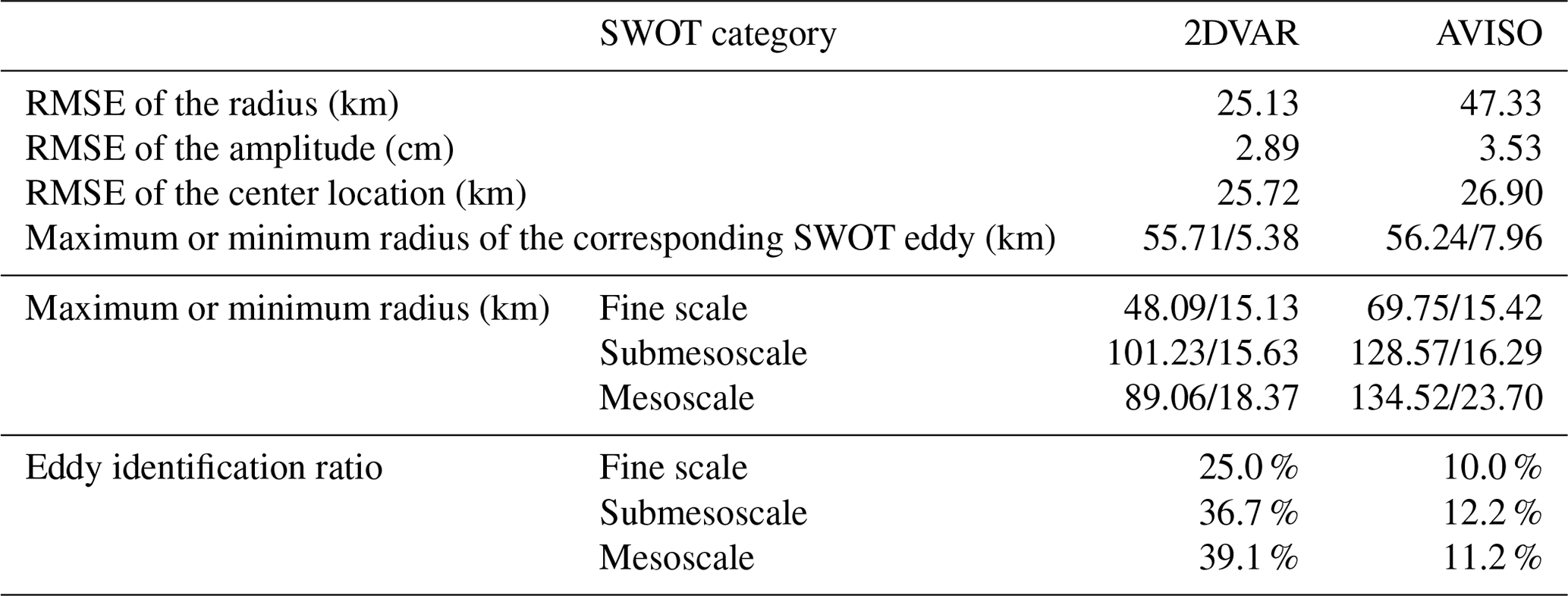
Note: in rows four and five, the “maximum or minimum radius” specifies the range of merged-map eddy radii for each SWOT category corresponding to Fig. 2, with the leading number being the maximum radius and the trailing number being the minimum radius.

3.2 Eddy boundary verification in space and time

This section presents a detailed visual display of merged-map eddies compared with SWOT eddies and eddy boundaries compared with drifter trajectories to further validate the reliability and accuracy of the identified eddies.

Figure 3 provides a detailed comparison of eddies from two merged maps using science-phase SWOT mission data in the central area of the SCS. The colored points in the figure show the Level-3 ADT observations directly from the KaRIn measurement on the SWOT satellite. A high degree of agreement was found between the eddies identified using 2DVAR and SWOT at scales ranging from 50 to 200 km. The 2DVAR product demonstrates strong agreement with the SWOT-derived anticyclonic eddies at 21° N, 116° E in Fig. 3a1, 17.5° N, 112° E and 16° N, 112° E in Fig. 3b1, and 18° N, 113° E in Fig. 3c1, together with the cyclonic eddy at 16.5° N, 111.5° E in Fig. 3b1. In contrast, the AVISO product fails to accurately match the cyclonic eddy at 16.5° N, 111.5° E with the SWOT observations in Fig. 3b2. Additionally, the AVISO product captures an eddy at 21° N, 116° E in Fig. 3a2 that only partially overlaps with the corresponding SWOT eddy, with minimal spatial correspondence. For other eddies where both merged products exhibit agreement, the radii of the AVISO eddies are notably larger than those identified by 2DVAR. Although the AVISO product exhibits lower consistency with SWOT observations compared to 2DVAR, it still captures a considerable number of eddies that align with SWOT, thereby maintaining its fundamental utility as a merged product for eddy identification. However, both products fail to detect certain small eddies in SWOT observations, such as the cyclonic eddy at 17° N, 112.5° E in Fig. 3c.

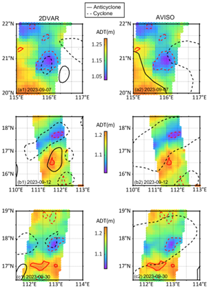
Figure 3 The ADT observation data of SWOT with the eddies detected by SWOT (in red), 2DVAR (in black, a1–c1), and AVISO (in black, a2–c2). The solid line represents the anticyclonic eddies, and the dashed line represents the cyclonic eddies.

It is important to emphasize that the examples presented in this section are representative of the eddy boundary reconstruction capabilities of both AVISO and 2DVAR. While these examples show that AVISO performs slightly worse than 2DVAR in terms of eddy radius and positional accuracy, they nonetheless represent some of the best-case scenarios for the AVISO product. This conclusion is not influenced by selective bias in the examples chosen but rather reflects the inherent performance differences between the two merged products, which is consistent with the statistical findings presented in Sect. 3.1.

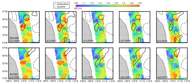
Figure 4 Observation data of SWOT (in red) with the 2DVAR (in black, a1–e1) and AVISO (in black, a2–e2) merged maps from 6 to 10 April 2023. The solid (dashed) line represents the anticyclonic (cyclonic) eddy, and the color-filled plot contains the KaRIn data from SWOT.

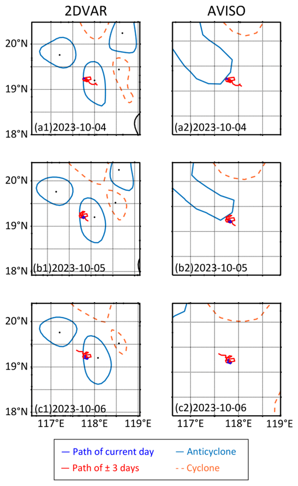
Figure 5 Trajectories of drifting buoys with 2DVAR (a1, b1, c1) and AVISO (a2, b2, c2) from 4 to 6 October 2023. The light-blue solid (orange dashed) line, dark-blue line segment, and red line segment represent the anticyclonic (cyclonic) eddies, the trajectory for the current day, and the trajectories for the 3 d before and after, respectively.

The CALVAL phase is utilized to capture the evolution of small-scale structures over time, as distinct from the science phase. A duration of 5 d was selected for this section, corresponding to the period of the fine-scale structure evolution.

On the 2DVAR maps, two closely spaced mesoscale anticyclones were identified at 15° N, 110° E and 16.2° N, 110.5° E in Fig. 4a1–e1, along with an anticyclone at 13.2° N, 110.5° E in Fig. 4b1, d1, and e1 and a smaller-scale cyclone at 14.8° N, 110.5° E in Fig. 4b1–e1. These eddies derived from 2DVAR exhibit discrepancies when compared to the SWOT-derived eddies, particularly in the case of the eddy at 16.2° N, 110.5° E, whose radius varies daily in the 2DVAR results and is represented by a colored circle on the map rather than as a distinct eddy in the SWOT data. Similar to Fig. 3, the 2DVAR method outperforms AVISO, which erroneously merges the two closely spaced anticyclones into a single larger eddy and fails to capture the eddies at 14.8° N, 110.5° E and 13.2° N, 110.5° E. Notably, by accurately matching the emergence and dissipation of SWOT eddies at 14.8° N, 110.5° E and 13.2° N, 110.5° E, the 2DVAR method demonstrates its ability to reconstruct eddies that evolve over time, despite some relative positional deviations from the actual eddy location.

Additionally, in the underlying SWOT data, although the algorithm fails to identify an eddy that is only partially within the swath, the color map reveals a noticeable expansion of the orange area on 7 April. This suggests that the anticyclone at this location is indeed larger in its spatial extent.

An example of the GDP drifter trajectories compared to the corresponding merged-map eddies is presented in Fig. 5. From 4 to 6 October 2023, an anticyclonic eddy was identified in the 2DVAR results at 19° N, 118° E, with a total of 7 d of drifter buoy trajectory segments within its boundaries. This indicates that the buoy was continuously rotating at a relatively fixed position for approximately 7 d. In contrast, AVISO failed to capture this anticyclonic eddy at the same location but instead identified a larger-scale anticyclonic eddy in the vicinity. This discrepancy highlights the accuracy and reliability of the mesoscale eddy detected by 2DVAR, despite a minor positional deviation.

Similar to Figs. 3 and 4, we have endeavored to select cases of eddy detection that are representative of both products. However, due to the limited spatial distribution and low observational frequency of the drifter data, the number of valid eddy detection cases available for analysis is highly constrained. In other instances, the differences between 2DVAR and AVISO in comparison with the drifter data are not significant (either both match the drifter trajectories or neither does). The case involving drifter 300534064134530 stands out as the only example demonstrating a clear and favorable comparison.

3.3 Eddy distribution and characteristics

In this section, we utilized data spanning several times the satellite observation period within the scientific phase, ensuring comprehensive coverage of the South China Sea region. Based on this dataset, we generated a distribution map of eddy characteristics. The eddy distributions and their tracks were mapped in Fig. 6 to provide a clearer representation of the identified eddies.

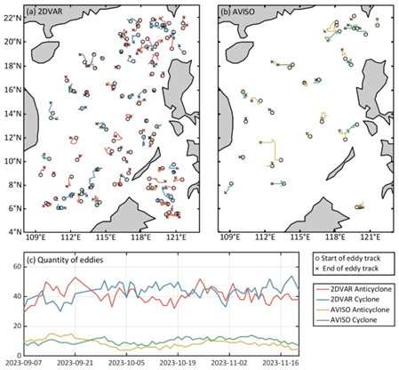
Figure 6 Eddies and tracks identified during the SWOT science phase (cycle numbers 3 to 6 and the time period from 6 September to 21 November 2023) on (a) 2DVAR and (b) AVISO merged maps. The red (yellow) and blue (green) lines represent the anticyclone and cyclone tracks on the 2DVAR (AVISO) merged maps. The black circles and crosses indicate the start and end positions of the eddies. (c) The number of eddies over time. The red (yellow) and blue (green) lines represent the daily count of anticyclones and cyclones, respectively, as identified on the 2DVAR (AVISO) merged maps.

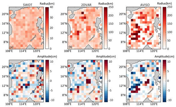
Figure 7 Distributions of the eddy radius (a, b, c) and amplitude (d, e, f) for SWOT (a, d), 2DVAR (b, e), and AVISO (c, f) from 6 September to 21 November 2023 are presented. The color intensity is proportional to the radius, with darker colors indicating larger radii. Similarly, the color intensity is proportional to the amplitude, with darker red (blue) indicating larger positive (negative) amplitudes.

The total number of anticyclones identified on the ADT merged maps was higher than that of cyclones, and the eddy tracks exhibited a northeast–southwest propagation and distribution pattern (Figs. 6a–b). This quantitative relationship and this distribution pattern are consistent between the two merged maps and are thought to be related to the path of eddies detached from the Kuroshio and intruding into the SCS via the Luzon Strait (at approximately 20° N, 121° E) (Huang et al., 2017; Jia and Chassignet, 2011). However, there was a significant discrepancy in the number of eddies identified by the two merged maps: 2DVAR identified approximately 4 times as many eddies as AVISO in terms of both the total number of eddies from September to November and the daily number of eddies (Fig. 6c). Notably, in the western part of the Luzon Strait, around 20° N, 119° E and below 12° N, 2DVAR identified a significantly greater number of eddies compared to AVISO.

The distributions of radius and amplitude for the eddies from merged maps and SWOT maps are displayed in Fig. 7. The radii of the eddies identified on the 2DVAR and AVISO maps are concentrated in the range 50–300 km (Fig. 7b–c), while the radii of the SWOT eddies are mostly under 50 km (Fig. 7a). This is partly due to the 120 km observation swath of SWOT, which restricts the capture of eddies larger than 120 km.

Larger mesoscale eddies were captured in the southwestern part of the SCS on the merged maps (Fig. 7b–c), whereas no eddies were observed on the SWOT maps (Fig. 7a). This is because eddies in this region may only exist at scales larger than the SWOT observation swath. Both merged maps captured a considerable number of larger mesoscale eddies with radii exceeding 200 km, which were more uniformly distributed in the northern and southwestern parts of the SCS, due to the influence of topographic effects (Su et al., 2020).

However, the radii of 2DVAR eddies are approximately 50–100 km smaller than those of AVISO, and a greater number of fine-scale and mesoscale eddies with radii below 150 km were captured in the central and southern parts of the SCS. This is due to the smaller effective resolution of 2DVAR (Liu et al., 2020).

The amplitudes of 2DVAR and AVISO are within ±10 cm, while the amplitudes of SWOT are within ±6 cm, which is 4 cm smaller than those of the merged maps in both the positive and negative directions.

4 Summary and discussion

This research leverages cutting-edge SWOT data to develop an advanced evaluation framework centered on eddy identification within merged maps, achieving superior validation abilities. Initially, the identified eddies are meticulously normalized and compared with actual eddies. Subsequently, eddy boundary details of the identified eddies are visually compared with those of the merged maps. Finally, the method is validated through observations, ensuring robustness and reliability. This comprehensive approach provides a rigorous assessment of the authenticity and precision of merged-map eddies, with a detailed analysis of the evaluation outcomes. The main outcomes are summarized as follows:

• The 2DVAR method has a fine-scale to mesoscale eddy identification ratio that is 2.5 to 4 times higher than that of AVISO and exhibits a 50 % improvement in the RMSE of eddy radii compared to AVISO, when validated against SWOT.

• Eddies identified in 2DVAR demonstrated superior coherence and agreement with SWOT data, especially for fine-scale eddies, compared to AVISO.

The results show that 2DVAR identified a significantly higher number of accurate fine-scale and mesoscale eddies compared to AVISO, which is consistent with earlier evaluations of 2DVAR in terms of the error analysis, wavenumber energy spectrum, effective resolution, and OSSE (Observing System Simulation Experiment) (Archer et al., 2020; Jiang et al., 2022). The effective resolution indicates the minimum spatial scale of signals that the merged maps can theoretically resolve, although it does not necessarily correspond to the actual minimum scale. The average effective resolution of AVISO in the SCS is approximately 150 km, whereas that of 2DVAR is about 80 km. This suggests that, typically, AVISO identifies larger eddies compared to 2DVAR. As a result, AVISO encounters greater limitations in identifying eddies across the mesoscale to fine-scale spectrum. Considering the small error correlation scales in high-eddy-kinetic-energy regions such as the South China Sea and other coastal areas, rational selection of the merged product's regional configuration is also very important. In terms of the tradeoff between result performances, the background field time window for AVISO is selected as a multiyear average field, which leads to an increase in the scale of the background error signals, and the scale of the signals will be amplified during the mapping process. Therefore, the merged map has difficulty in reconstructing and identifying small-scale processes such as small-scale eddies and will identify more large and mesoscale eddies. Due to the narrow swath of the SWOT track, the number of large and mesoscale eddies that can be identified by AVISO within this range is limited, which may ultimately lead to the limited number of eddies detected by AVISO. In contrast, 2DVAR adopts a 1 d background field time window, and the reduction in background error correlation scales allows for the reconstruction of more fine-scale to mesoscale signals.

The successful matches with SWOT eddies on scales of less than 20 km further support the argument that fine-scale to mesoscale eddies may have been overlooked on the merged maps. To be noticed, the results shown in this research should be interpreted as the best-case scenario because the eddy identification used for the 2DVAR, AVISO, and SWOT maps was identical, implying that the method is perfect. However, several deficiencies may cause errors, including inappropriate eddy determinations on daily maps without matching with track results. This is because the eddies move tens of kilometers a day, which is almost the same as with the SWOT swath, resulting in short-trajectory eddies being incorrectly determined as actual eddies on SWOT or merged maps. Also, ignorance of non-closure of contour lines on SWOT maps might be a deficiency. Most of the eddy scales on the SWOT maps do not exceed 50 km, which limits their ability to fully represent mesoscale eddies, especially those larger than 50 km. Additionally, despite being accurate in terms of radius scale and boundary detail, a significant discrepancy remains in terms of positional deviation, which may result in a false match between merged-map eddies and actual eddies. To address method deficiencies, one possible avenue for improvement would be to use AI or machine learning algorithms for eddy identification and matching, along with auto-tracking algorithms to select eddies that persist over time within a limited swath. Compared to the GDP, the validation capability of SWOT is enhanced in both temporal and spatial aspects. This is due to the high cost and sparse distribution of drifter platform observations. In contrast, the CALVAL phase of SWOT provided a robust dataset for studying small-scale dynamical structures over time. SWOT has now entered the official operational phase, which means that it will no longer provide regionally repetitive data of 1 d rapid sampling, and the data from the CALVAL phase have become particularly valuable.

The innovative approach presented in this research optimizes and broadens the applications for SWOT data, marking an advancement in the assessment of dynamic signals at the sea surface, particularly at the fine scale. Traditional nadir altimeters, due to their linear single-point sampling method, lack the ability to identify ocean eddies, which have a two-dimensional structure. Therefore, compared to traditional nadir altimeters, the advantage of SWOT lies in its ability to quantitatively analyze the observable scales of two-dimensional structures, such as eddies, within the study area. Since the SWOT data have proven their ability to represent fine-scale eddies through in situ calibration experiments (Zhang et al., 2024), they can be used as input information for the 2DVAR merging method in the future. With the release of the latest available data, our research will continue to leverage SWOT to enhance merging methodologies and validate sea surface dynamical structures. The combination of SWOT and 2DVAR will theoretically help improve the effective resolution and accuracy of the merged maps, and this work can provide technical support for oceanographic understanding and prediction capabilities.