An emerging pathway of Atlantic Water to the Barents Sea through the Svalbard Archipelago: drivers and variability

The Barents Sea, an important component of the Arctic Ocean, is experiencing changes in its ocean currents, stratification, sea ice variability, and marine ecosystems. Inflowing Atlantic Water (AW) is a key driver of these changes. As AW predominantly enters the Barents Sea via the Barents Sea Opening, other pathways remain relatively unexplored. Comparisons of summer climatology fields of temperature from the last century with those from 2000–2019 indicate warming in the Storfjordrenna trough and along two shallow banks, Hopenbanken and Storfjordbanken, within the Svalbard Archipelago. Additionally, they indicate shoaling of AW that extends further into the “channel” between the islands of Edgeøya and Hopen. This region emerges as a pathway enabling AW to enter the northwestern Barents Sea. Moreover, 1-year-long records from a mooring deployed between September 2018 and November 2019 at the saddle of this channel show the flow of Atlantic-origin waters into the Arctic domain of the northwestern Barents Sea. The average current is directed eastwards into the Barents Sea and exhibits significant variability throughout the year. Here, we investigate this variability on timescales ranging from hours to months. Wind forcing mediates currents, water exchange, and heat exchange through the channel by driving geostrophic adjustment to Ekman transport. The main drivers of the warm-water inflow and across-saddle transport of positive temperature anomalies include persistently strong semidiurnal tidal currents, intermittent wind-forced events, and wintertime warm-water intrusions forced by upstream conditions. We propose that similar topographic constraints near AW pathways may become more important in the future. Ongoing warming and shoaling of AW, coupled with changes in large-scale weather patterns, are likely to increase warm-water inflow and heat transport through the processes identified in this study.

1 Introduction

The shallow Barents Sea (Fig. 1) plays a crucial role in the Arctic climate system, serving as one of the two main gateways enabling Atlantic Water (AW) to enter the Arctic Ocean (e.g. Schauer et al., 2002; Smedsrud et al., 2013). Recent “Atlantification” of the Arctic Ocean (Årthun et al., 2012; Polyakov et al., 2017), characterised by ocean warming, weakening stratification, and declining winter sea ice (Shu et al., 2021), is partly driven by AW circulating through the Barents Sea (e.g. Asbjørnsen et al., 2020). The largest volume of AW enters the Barents Sea through the Barents Sea Opening (BSO; Fig. 1). In addition, AW can enter the northwestern Barents Sea through the Northern Barents Sea Opening (Lind and Ingvaldsen, 2012; Lundesgaard et al., 2022) via the branch that enters the Arctic Ocean through the Fram Strait and extends north of Svalbard (e.g. Lind and Ingvaldsen, 2012). As AW flows through the Barents Sea, it is modified and transformed due to intense cooling resulting from heat loss to the atmosphere (Häkkinen and Cavalieri, 1989; Årthun and Schrum, 2010; Lind et al., 2018; Ivanov et al., 2020); brine release from sea ice growth (e.g. Schauer et al., 2002; Ivanov et al., 2020); mixing with Arctic Water, which is cooler and fresher (Loeng, 1991; Lind et al., 2018); and mixing with denser, brine-enriched waters (Schauer et al., 2002). The Barents Sea has been termed a “cooling machine” (Smedsrud et al., 2013), where AW is transformed into Barents Sea water. It is an important area of dense-water production (Knipowitsch, 1905; Midttun, 1985; Schauer et al., 2002; Årthun et al., 2011) and a source of intermediate waters for the Arctic Ocean (Rudels et al., 1994; Schauer et al., 1997, 2002; Rudels et al., 2013).

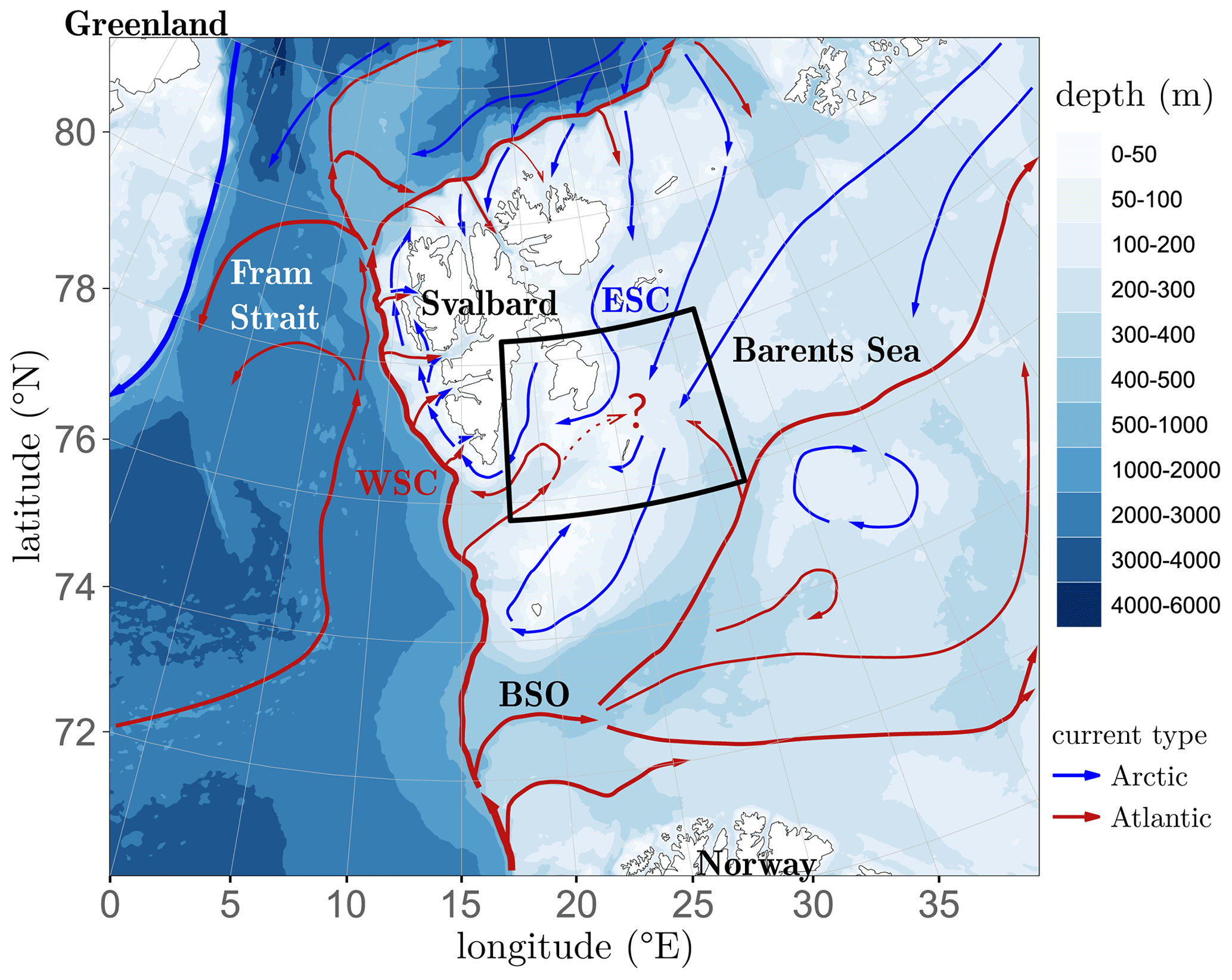
Figure 1 Bathymetry in the western Barents Sea and the Fram Strait (version 3 of the International Bathymetric Chart of the Arctic Ocean (IBCAO); Jakobsson et al., 2012) is shown along with general circulation (solid arrows; Vihtakari et al., 2019, adapted from Eriksen et al., 2018). The West Spitsbergen Current (WSC), the East Spitsbergen Current (ESC), and the Barents Sea Opening (BSO) are marked. The black rectangle indicates the area shown in the detailed map in Fig. 2. The map was prepared using PlotSvalbard (Vihtakari, 2020), which uses data originating from the Norwegian Polar Institute (© Norsk Polarinstitutt, https://npolar.no, last access: 30 July 2024).

Large-scale environmental changes have been observed in the Barents Sea over the past decades (Oziel et al., 2016; Skagseth et al., 2020; Isaksen et al., 2022; Smedsrud et al., 2022). The loss of winter sea ice in the Arctic in recent times has been most pronounced in the Barents Sea (Onarheim and Årthun, 2017; Rieke et al., 2023), which is the first Arctic sea projected to be ice-free throughout the entire year (Årthun et al., 2021). Increased heat transport through the BSO is an important driver of sea ice loss and warming in the Barents Sea, and it also significantly contributes to its Atlantification (Årthun et al., 2012; Asbjørnsen et al., 2020). Increasing air temperatures also drive sea ice loss. In the northern Barents Sea, surface air temperatures have risen twice as fast as in the Arctic as a whole (Isaksen et al., 2022). Decreased import of sea ice into the northern Barents Sea is another factor in the increased sea ice loss (Lind et al., 2018; Ingvaldsen et al., 2021), resulting in reduced freshwater input and a weakening of the stratification (Lind et al., 2018). The weakening stratification facilitates enhanced vertical mixing and increased heat fluxes, which may further inhibit sea ice formation (Lind et al., 2018). Further hydrographic changes in the Barents Sea include increased salinity; a diminishing presence of Arctic Water (Lind et al., 2018); changes in the polar front (Barton et al., 2018; Kolås et al., 2023), which marks the boundary between waters of Atlantic and Arctic origins; and a poleward shift in the region where the cooling machine is efficient (Skagseth et al., 2020; Shu et al., 2021).

The Atlantification of the Barents Sea presents major consequences for the ecosystem (Gerland et al., 2023), such as increased production, the northward expansion of boreal species, a reduction in ice-associated ecosystem compartments, and increased connectivity within the food web (Ingvaldsen et al., 2021). Net primary production in the Barent Sea has increased substantially over the past 2 decades (Dalpadado et al., 2020; Lewis et al., 2020). Boreal zooplankton have expanded northwards (Geoffroy et al., 2018), while some Arctic zooplankton species have retreated (Eriksen et al., 2017). The northward expansion of Atlantic zooplankton species is expected to continue, potentially impacting Arctic zooplankton communities (Wold et al., 2023). Changes in biomass and distribution have also been observed higher up the food web (Gerland et al., 2023, and references therein).

Although the BSO is the main gateway enabling AW to enter the Barents Sea, other inflow regions, such as the Northern Barents Sea Opening, may be important. Furthermore, as the West Spitsbergen Current (WSC) transports AW northwards towards the Fram Strait, some of this AW is directed into the Storfjordrenna trough in the Svalbard Archipelago (Fig. 2), located north of the BSO and the shallow bank Spitsbergenbanken. In the Storfjordrenna trough, AW flows cyclonically, guided by the topography, with shallow areas situated to its right (Schauer, 1995; Vivier et al., 2023).

The Storfjordrenna trough experienced a positive sea surface temperature (SST) trend from 1982 to 2020, with the largest SST increase in the Barents Sea occurring between 1995 and 2007 (Mohamed et al., 2022b). This increase was due to the greater inflow of AW following shallower isobaths compared to earlier periods. Following a year of record-low sea ice cover, the surface layers in Storfjorden and the Storfjordrenna trough were replaced by warmer and more saline Arctic Water during the summer of 2016 (Vivier et al., 2023). The summer of 2016 saw the warmest and longest-lasting marine heatwave in the Barents Sea to date (Mohamed et al., 2022a).

Northeast of the Storfjordrenna trough, on the Arctic side of the polar front, lies the Olga Basin (Fig. 2). Here, the Arctic Water layer is the coldest and thickest compared to other parts of the northern Barents Sea (Lind and Ingvaldsen, 2012). Arctic Water enters through the gaps and troughs in the northern Barents Sea (Dickson et al., 1970; Loeng, 1991) and circulates with the East Spitsbergen Current (Quadfasel et al., 1988; Loeng, 1991). In addition to Arctic Water, AW enters the Olga Basin at depth through the gateways to the north (Lind and Ingvaldsen, 2012; Lundesgaard et al., 2022) and, to a lesser extent, over the ≈200 m deep saddle separating the Olga Basin from the Hopendjupet trench to the south (Kolås et al., 2023; Lind and Ingvaldsen, 2012) (Fig. 2).

The channel between the islands of Edgeøya and Hopen (Fig. 2) separates the increasingly warm and shoaling AW in the Storfjordrenna trough from the Olga Basin, which is the Arctic domain in the northwestern Barents Sea. Here, we investigate the physical processes that drive and mediate the inflow of Atlantic-origin waters into the Olga Basin. Such warm-water inflow has the potential to reduce sea ice growth, accelerate melt, and alter deep-basin stratification in the Olga Basin. The (increasing) presence of warm Atlantic-origin waters in the Storfjordrenna trough may also impact the properties of the East Spitsbergen Current as it crosses the channel westwards, as well as those of Storfjorden and the coastal environment west of Spitsbergen. We propose that the study site may become an increasingly relevant pathway for warm waters travelling into the Arctic domain of the Barents Sea. Using novel data from a less-explored region, we identify and discuss the variability in currents and heat exchange on timescales ranging from hours to months.

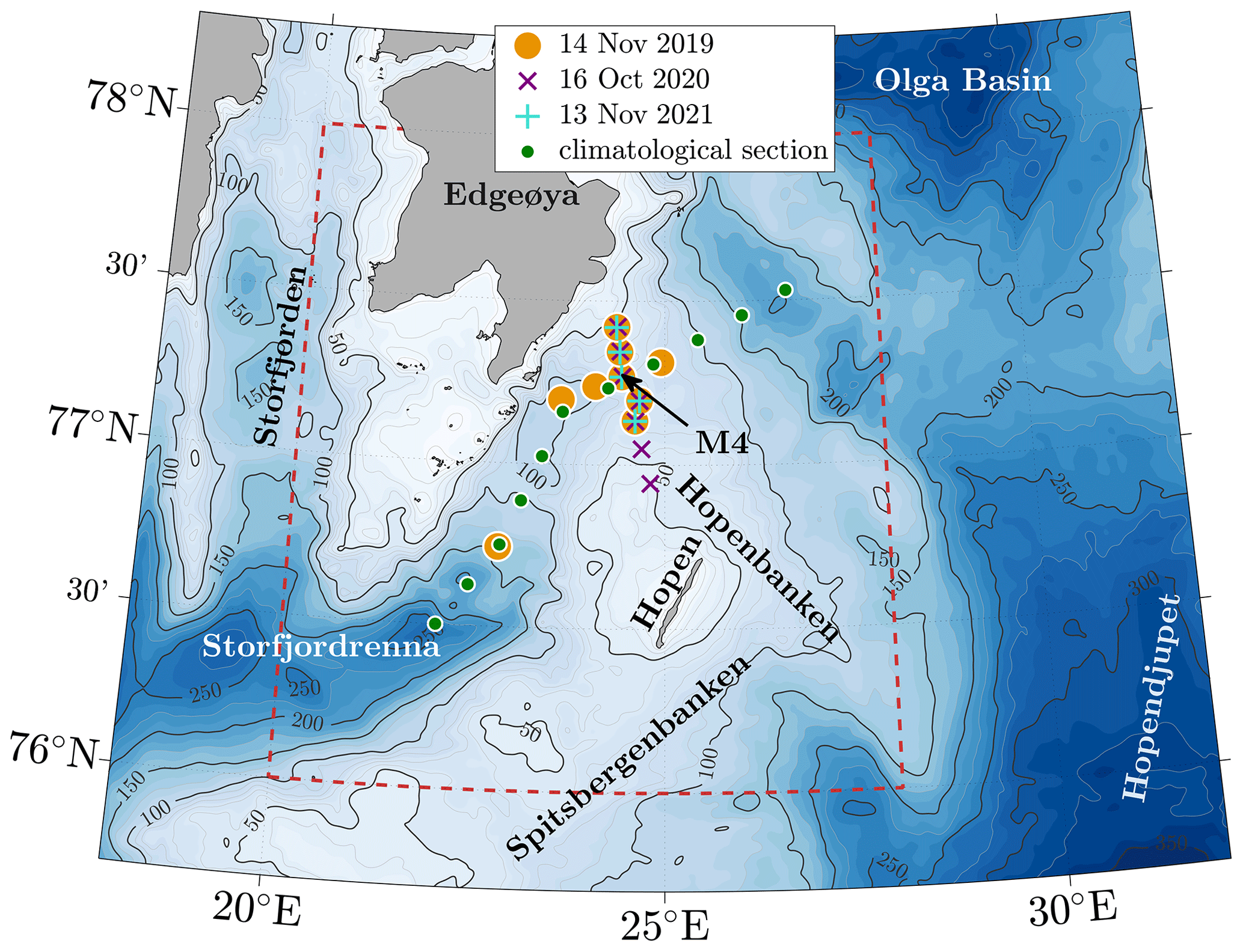
Figure 2 Bathymetry in the mooring area (IBCAO version 4; Jakobsson et al., 2020). The M4 mooring site (black arrow) is located at the saddle of Hopenbanken between the Storfjordrenna trough and the interior of the northwestern Barents Sea. The saddle is flanked to the north and south by the islands of Edgeøya and Hopen, respectively. Hydrographic stations from 14 November 2019, 16 October 2020, and 13 November 2021, as well as the climatological section in Fig. 4, are marked (see legend). The dashed red rectangle indicates the area illustrated in Fig. 3.

2 Data and methods

2.1 Data

In this study, we use a combination of historical hydrographic data, recent hydrographic transects collected during late autumn, and year-long current and hydrography time series from a mooring. The mooring was deployed at 70 m depth on Hopenbanken, a shallow bank, between the Storfjordrenna trough and the interior of the Barents Sea (Fig. 2).

The historical data include hydrographic profiles extracted from the University Centre in Svalbard (UNIS) Hydrographic Database (UNIS HD; Skogseth et al., 2019), covering the vicinity of the mooring area from 1930–2019.

Recent hydrographic transects were collected on 14 November 2019 aboard Kronprins Haakon (Sundfjord and Renner, 2021), on 16 October 2020 aboard G. O. Sars (Fer et al., 2021), and on 13 November 2021 aboard Kronprins Haakon (Renner and Sundfjord, 2022).

From 29 September 2018 to 14 November 2019, temperature, salinity, and ocean currents were measured using instruments on the mooring located at 77°16.116^′ N, 24°24.402^′ E (Fig. 2). The mooring was a trawl-proof bottom frame equipped with one conductivity–temperature–depth (CTD) recorder (Sea-Bird MicroCAT SBE 37-SM (unpumped)) and one acoustic Doppler current profiler (ADCP; Nortek Signature250), both housed within the frame with transducers pointing upwards. The MicroCAT instrument recorded temperature, salinity, and pressure near the bottom (at about 68 m) for the entire period at a sampling interval of 15 min. The ADCP profiled current speed and direction through the water column using 25 cells with a thickness of 3 m at an averaging interval of 20 min. All data from the mooring were interpolated onto a common hourly time vector prior to analysis.

We corrected the velocity direction for a magnetic declination of 15°. The ADCP compass was further validated by comparing the tidal ellipses obtained from the observed current velocity with those from the Arctic Ocean Tidal Inverse Model on a 5 km grid, developed in 2018 (Arc5km2018) (Erofeeva and Egbert, 2020). For the M₂ tidal constituent, the ellipse inclinations from Arc5km2018 and the depth-averaged measured current were approximately the same. For the other significant semidiurnal constituents (S₂, N₂, and K₂), the ellipse properties from the measured currents were in fairly good agreement with Arc5km2018 – i.e. ellipse inclinations agreed within 14°, and semi-major axes agreed within 1 cm s⁻¹. Since M₂ is the dominant constituent in the study area, no further compass corrections were deemed necessary. We then referenced the current velocity profiles to the surface to account for sea-level variations detected by the ADCP's altimeter.

We extracted data on wind speed and direction for the region from the ERA5 reanalyses – this included hourly data on single levels with a spatial resolution of 0.25° (Hersbach et al., 2020). Additionally, we extracted data on sea surface temperature (SST) and sea ice concentration (SIC) from the Global Ocean OSTIA Sea Surface Temperature and Sea Ice Reprocessed product, which comprises daily data with a spatial resolution of 0.05° (OSTIA, 2023; Good et al., 2020).

All data used in this study are openly available, as detailed in the “Data availability” section.

2.2 Data analysis methods

The historical hydrographic data (Skogseth et al., 2019) have been optimally interpolated onto horizontal and vertical climatological sections to compare data from the past 2 decades (2000–2019) to data from the previous century (1930–2000). Due to the temporally and spatially sparse data coverage, only summer (July–October mean) sections were created. A description of gridding and interpolation, along with details on data coverage and standard deviations for the climatological maps and vertical sections, is given in Appendix A.

Temperature and practical salinity from the recent hydrographic transects, the mooring, and the optimally interpolated climatological sections were converted to Conservative Temperature and Absolute Salinity, respectively, following the Thermodynamic Equation of Seawater – 2010 (TEOS-10) (Mcdougall and Krzysik, 2015). In the following, we use the subscript “b” (for bottom) to refer to temperature T_b and salinity S_b near the seafloor. AW is defined as water with Conservative Temperature Θ≥2 °C and Absolute Salinity $S_{\mathrm{A}}\ge \mathrm{35.06}\mathrm{g}{\mathrm{kg}}^{-\mathrm{1}}$ (Sundfjord et al., 2020). We refer to Atlantic-origin waters as AW that is modified or transformed en route from the WSC through the Storfjordrenna trough into relatively warm and saline water compared to the surrounding water masses; however, it is colder and less saline than pure AW. This inflow of warm water into the Barents Sea affects deep-basin stratification and sea ice growth and melt.

We identify the timescales of variability using spectral analysis. Cartesian and rotary spectral components were estimated following the multitaper method from Percival and Walden (1993), with Slepian data tapers applied (e.g. Slepian, 1978; Thomson, 1982). To analyse the time variability in the spectral components, we used wavelet transforms following Lilly and Olhede (2009), employing generalised Morse wavelets (Olhede and Walden, 2002). The values for the parameters defining the Morse wavelets were set as γ=3 for symmetric wavelets and β=5 to resolve variability in both frequency and time on timescales ranging from semidiurnal to a few weeks.

The spectral analysis revealed three frequency bands with dominant variability: semidiurnal tides (periods of 10 to 14 h), “weather-band” processes (28 h to 10 d), and lower-frequency activity (7 d to 6 weeks). To study these fluctuations, we filtered the time series with a Butterworth band-pass filter. We used the highest possible order while ensuring stability for each frequency band – i.e. we employed an order of 5 for semidiurnal tides and weather-band processes and used an order of 3 for lower-frequency activity.

To describe and visualise the background conditions in hydrography and currents, we used a low-pass Butterworth filter with an order of 6 and a cutoff frequency corresponding to 10 d.

We analysed the current velocity data from the mooring to study the mean flow properties and flow variability over timescales associated with tidal variability, weather-band processes, and lower-frequency events. For this, we used two different coordinate system rotations. The coordinate system was rotated by −42° to align with the long-term mean flow along the isobaths. The rotated velocity components are denoted as u_R and v_R for the along-isobath (roughly southeast) and across-isobath (roughly northeast) directions, respectively. To analyse variability at selected timescales, we applied another rotation to the velocity components, denoted as u_r and v_r. These components were oriented along and across the direction of the highest variance within the frequency bands associated with weather-band processes and lower-frequency activity. This coordinate system was rotated by −28°, orienting u_r roughly towards the east-southeast and v_r towards the north-northeast.

Eddy temperature fluxes were calculated as $\stackrel{\mathrm{‾}}{{u_{\mathrm{r}}}^{\prime }{T}^{\prime }}$ and $\stackrel{\mathrm{‾}}{{v_{\mathrm{r}}}^{\prime }{T}^{\prime }}$, where T^′ denotes fluctuations in near-bottom temperature and ${u_{\mathrm{r}}}^{\prime }$ and ${v_{\mathrm{r}}}^{\prime }$ are the velocity component fluctuations along (−28° relative to east) and across (62° relative to east) the direction of highest variance in the frequency bands associated with weather-band processes and lower-frequency activity. The fluctuations (denoted by primes) were obtained by applying a band-pass filter to the time series. The velocity data were layer-averaged over the bottom half of the water column. Although the water column was at times stratified in temperature, available CTD profiles suggest that the lower half of the water column was typically well mixed. Therefore, temperature measurements recorded close to the bottom may be considered representative of the lower half of the water column. The overline denotes a 30 d moving average.

The wind stress vector was calculated as $\mathit{\tau }=({\mathit{\tau }}_x,{\mathit{\tau }}_y)={\mathit{\rho }}_{\mathrm{air}}{C}_{\mathrm{D}}\left|{\mathit{u}}_{\mathrm{10}\mathrm{m}}\right|(u_{\mathrm{10}\mathrm{m}},v_{\mathrm{10}\mathrm{m}})$, where ${\mathit{\rho }}_{\mathrm{air}}=\mathrm{1.25}\mathrm{kg}{\mathrm{m}}^{-\mathrm{3}}$, representing the density of air; ${\mathit{u}}_{\mathrm{10}\mathrm{m}}=(u_{\mathrm{10}\mathrm{m}},v_{\mathrm{10}\mathrm{m}})$, denoting the wind vector with eastward and northward components of wind velocity at 10 m, extracted from ERA5; $\left|{\mathit{u}}_{\mathrm{10}\mathrm{m}}\right|$ is the magnitude of the wind velocity; and C_D is the drag coefficient. We used C_D values that depend on sea ice concentration, following Lüpkes and Birnbaum (2005). Ekman transport was calculated from the wind stress using $(U_{\mathrm{E}},V_{\mathrm{E}})=\frac{\mathrm{1}}{{\mathit{\rho }}_{\mathrm{0}}f}({\mathit{\tau }}_y,-{\mathit{\tau }}_x)$, where ${\mathit{\rho }}_{\mathrm{0}}=\mathrm{1027}\mathrm{kg}{\mathrm{m}}^{-\mathrm{3}}$, indicating the reference density of seawater, and f is the Coriolis parameter.

Time series of SST, SIC, wind velocity, and wind stress at the mooring location were obtained by spatially interpolating onto the mooring location from the original grids, i.e. from 0.05° for SST and SIC and from 0.25° for wind velocity and wind stress.

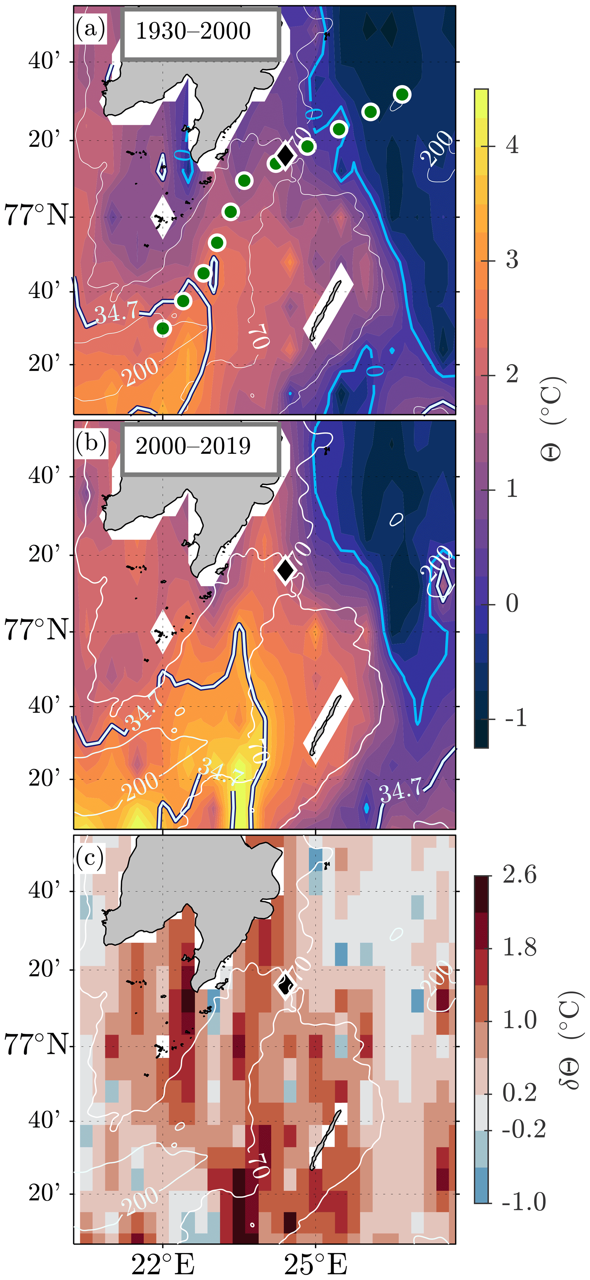
Figure 3 Climatological maps illustrating depth-averaged Conservative Temperature Θ (°C) with respect to (a) 1930–2000, (b) 2000–2019, and (c) the difference between the two periods (1930–2000 subtracted from 2000–2019). In panels (a) and (b), the 0 °C isotherm (blue) and the 34.7 g kg⁻¹ isohaline (pale blue) are shown for reference. In panel (a), the vertical section depicted in Fig. 4 is marked with green dots, and the mooring position is indicated by a black diamond. The 70 and 200 m isobaths are outlined with white contours.

3 Results

3.1 Long-term changes in the hydrographic environment of the Storfjordrenna trough and Hopenbanken

The hydrographic environment in the Storfjordrenna trough and the shallow banks Hopenbanken and Storfjordbanken (Fig. 2) has experienced warming over the past 2 decades. Summer climatology maps of depth-averaged temperature from 1930–2000 (Fig. 3a) and 2000–2019 (Fig. 3b) indicate warming across most of the area. The observed increase in average temperature exceeds 1 °C over large parts of Hopenbanken and Storfjordbanken (Fig. 3c). This warming is observed both at the surface and at depth (not shown). The 34.7 g kg⁻¹ isohaline extended further northeastwards in 2000–2019 compared to 1930–2000 (Fig. 3a and b).

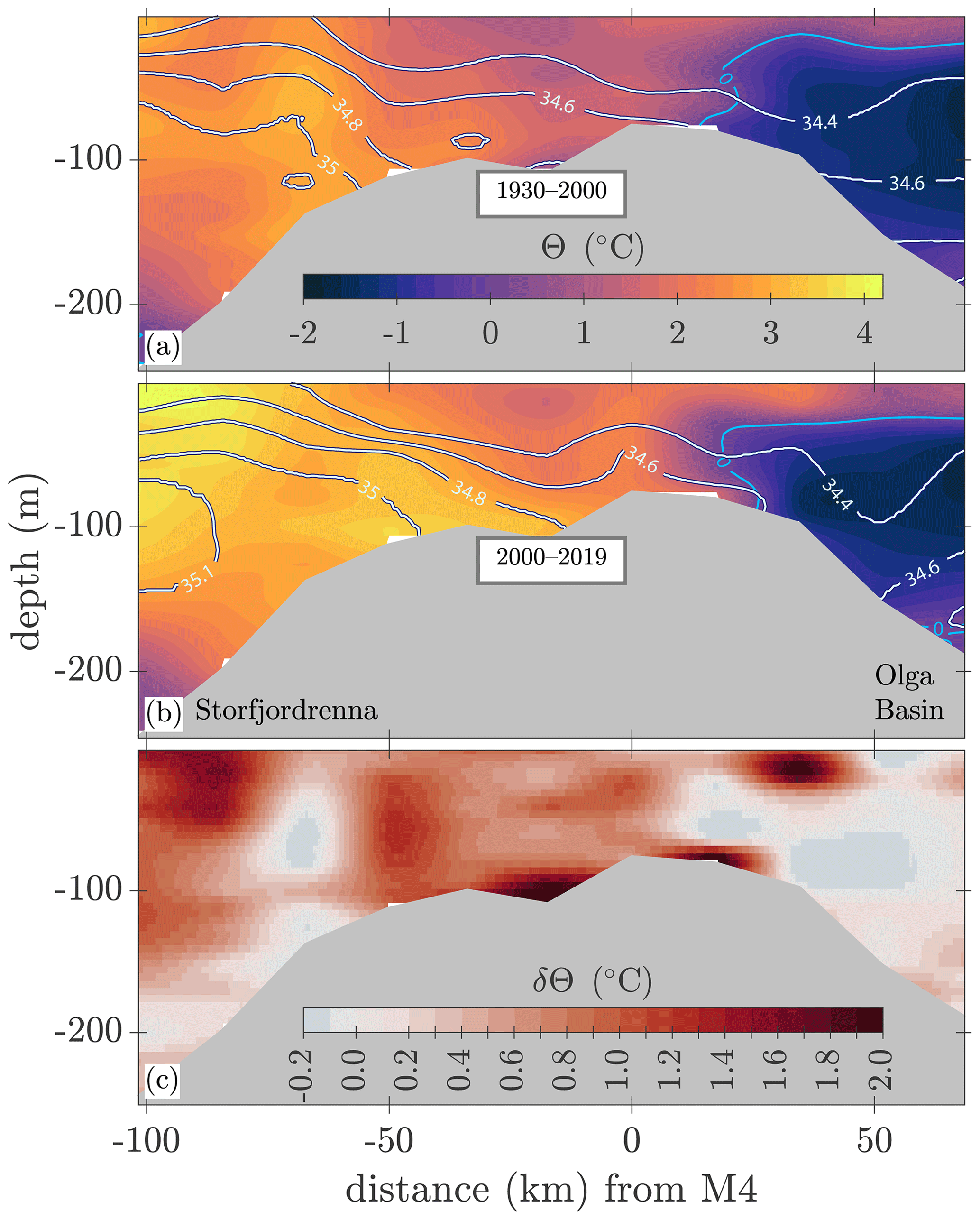
Figure 4 Vertical climatological hydrographic sections extending from the Storfjordrenna trough, across the saddle, and into the Olga Basin with respect to (a) 1930–2000, (b) 2000–2019, and (c) the difference between the two periods (1930–2000 subtracted from 2000–2019). (a, b) Conservative Temperature Θ (°C) is depicted using various colours, and the 0 °C isotherm is highlighted in blue. The isohalines corresponding to 34.4, 34.6, 34.8, 35.0, and 35.1 g kg⁻¹ are shown as pale-blue curves. (c) The difference in Conservative Temperature δΘ (°C) is depicted using various colours. The x axis shows the distance from the mooring position, with positive values indicating the direction towards the Olga Basin. The location of this section is marked with green dots in Fig. 3a.

Vertical climatological sections extending from the Storfjordrenna trough, across the saddle on Hopenbanken, and into the Olga Basin (Fig. 4) show that Atlantic-origin waters have shoaled in the water column and now extend further east towards the saddle. This warming has occurred throughout the water column, and the saddle area has warmed by 1 to 2 °C. Additionally, salinity has increased by 0.05 to 0.35 g kg⁻¹ over intermediate depths in the Storfjordrenna trough (not shown). We also note that the past 2 decades has seen a deepening of the 34.4 g kg⁻¹ isobath and a corresponding decrease in temperature towards the Olga Basin (Fig. 4b and c).

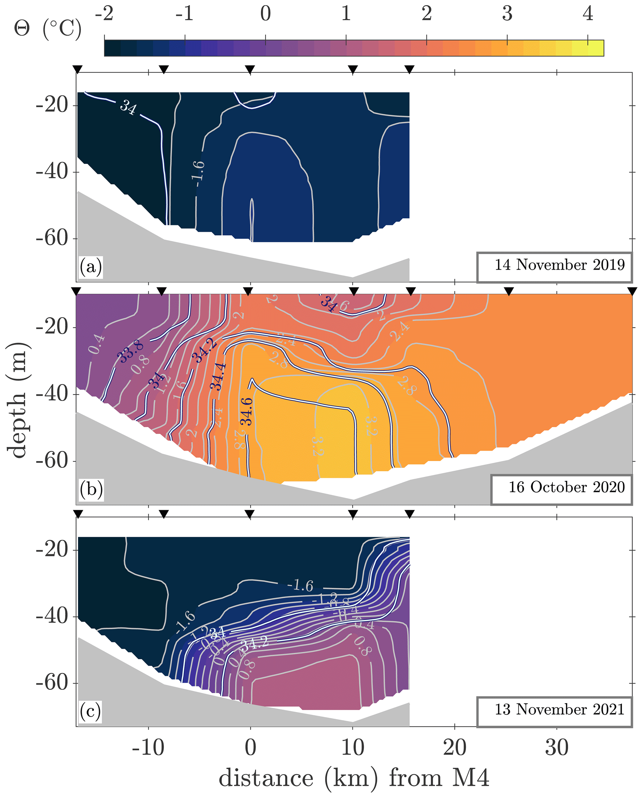
Figure 5 Hydrographic transects along the saddle between the Storfjordrenna trough and the Barents Sea from (a) 14 November 2019, (b) 16 October 2020, and (c) 13 November 2021. Conservative Temperature is shown using various colours (contours depicted every 0.2 °C), and Absolute Salinity is depicted using pale-blue contours (every 0.2 g kg⁻¹). The northern part of the saddle (close to Edgeøya) is on the left, and the southern part (towards Hopen) is on the right. The x axis shows the distance to the M4 mooring site, with positive values indicating the direction towards the south.

3.2 Late-autumn hydrographic transects indicate large variability

Recent hydrographic transects from the saddle region, collected in November 2019, October 2020, and November 2021 (Fig. 5), show that the mooring is situated in an area with notable thermal and haline gradients. Local maxima in temperature and salinity were observed near the mooring position in late autumn.

In November 2019, the transect along the saddle was cold and relatively fresh but retained some heat (Fig. 5a). The warmest water (−1.2 °C) was found by the mooring position in the lower half of the water column. On the northern side of the transect, temperatures were near the freezing point, accompanied by relatively high salinity (Fig. 5a). At this time, AW was present in the Storfjordrenna trough and close to the mooring (not shown). Specifically, 70 km southwest of the mooring, water temperatures ranging from 2.9 to 3.7 °C and salinity between 34.84 and 35.02 g kg⁻¹ were found at depth. These temperatures are within the range for pure AW, but the salinities are slightly lower than the threshold of 35.06 g kg⁻¹ (Sundfjord et al., 2020). Additionally, relatively warm water (around 0.5 °C) was detected at a depth of 10 km to the west of the mooring position.

In October 2020, warm and saline water of Atlantic origin occupied the lower half of the water column (Fig. 5b). The warmest water, with a temperature of 3.3 °C and a salinity of 34.6 g kg⁻¹, was located 10 km south of the mooring position. Water warmer than 2 °C reached the surface at the mooring position and also between 15 and 37 km south of the mooring position. The coolest and least saline water was found on the northern side of the transect. At a station located 60 km to the northeast, we observed water with a temperature of 1 °C and a salinity of 35.0 g kg⁻¹ below 150 m depth (not shown).

In November 2021, a maximum temperature of 1 °C was found at (and south of) the mooring position (Fig. 5c), which was warmer than the maximum temperature in November 2019 (Fig. 5a). The isohalines were also aligned with the isotherms, with salinities exceeding 34.2 g kg⁻¹ for water at depth with temperatures ≥0 °C on the southern side. The northern side of the transect remained below −1.75 °C, consistent with observations from November 2019.

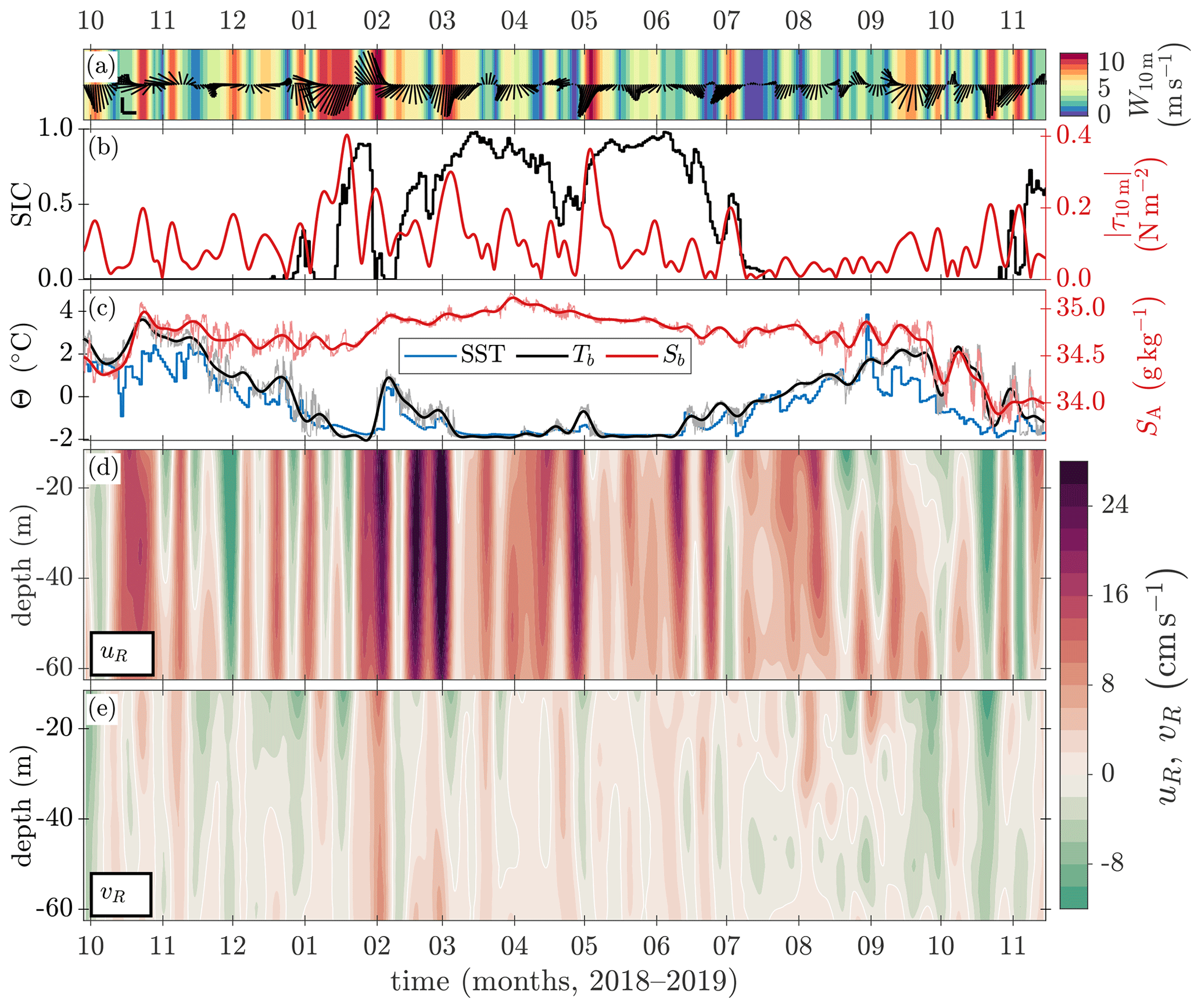
Figure 6 Time series for the mooring deployment period (29 September 2018 to 14 November 2019) illustrating (a) wind speed (coloured areas) and wind velocity (where quivers are depicted every 24 h, an upward-pointing vector represents wind blowing northwards, and reference quivers correspond to 5 m s⁻¹); (b) SIC, shown in black (left y axis), and wind stress τ_10 m (N m⁻²), shown in red (right y axis); (c) Conservative Temperature Θ (°C) near the seabed (black), SST (°C; blue), and Absolute Salinity S_A (g kg⁻¹) near the seabed (red; right y axis); (d) the along-isobath velocity component u_R at −42° (directed southeastwards); and (e) the across-isobath velocity component v_R at 48° (directed northeastwards). Wind velocity, wind stress, mooring temperature and salinity, and current velocity are low-pass-filtered with a cutoff frequency corresponding to 10 d. T_b and S_b are presented as both unfiltered (thin pale curves) and low-pass-filtered (thick dark curves). SST and SIC are given in terms of daily values. Wind velocity, SST, and SIC were spatially interpolated onto the mooring position.

3.3 Seasonal variability in hydrography and current velocity from mooring records

Early in the record, both near-bottom temperature, T_b, and salinity, S_b, increased, reaching values approaching those of pure AW properties by the middle of October (Fig. 6c). Near-bottom temperature was higher than SST, and the increase in T_b and S_b coincided with a relatively strong and long-lasting surface-intensified current directed southeastwards along the isobath (u_R; Fig. 6d). Following the maxima in near-bottom temperature and salinity, the water column gradually cooled until mid-January 2019, when both T_b and SST nearly reached the freezing point (Fig. 6c). During these months, u_R oscillated between −5 and 10 cm s⁻¹ on a 2-week timescale, with negligible depth variability over the measured range (Fig. 6d). Temperature and salinity co-varied with u_R, with T_b and S_b lagging behind u_R by 3.3 and 4.8 d, respectively. Sea ice was first observed across the saddle in late December (Fig. 6b).

From mid-January to mid-June 2019, there was partial sea ice cover across the saddle (Fig. 6b). Additionally, T_b and SST were generally at or close to the freezing point (Fig. 6c). S_b increased, probably as a result of brine release from sea ice formation, reaching its highest value (35.12 g kg⁻¹) by the end of March, and then gradually decreased (Fig. 6c). During this time, the current was more unidirectional than during autumn – i.e. u_R was generally positive (Fig. 6d) and typically varied between 5 and 10 cm s⁻¹, occasionally exceeding 20 cm s⁻¹.

Although the saddle was covered in ice and the water was generally near the freezing point during winter and spring, there were several episodes when T_b and SST increased. These increases coincided with a reduction in SIC and an enhancement of u_R (Fig. 6b–d). The first and largest increase in T_b and SST occurred in early February 2019, following a sharp reduction in SIC at the end of January. During this period, sea ice cover that had built up over 2 weeks due to northerly winds disappeared within 2 d. The wind shifted to a southerly direction, and u_R values became positive shortly before the sea ice disappeared from the saddle (Fig. 6a and d). The surface-intensified u_R increased in strength during and after the sea ice disappearance, reaching a maximum of 26 cm s⁻¹ close to the surface (Fig. 6d). T_b and SST increased to 0.9 and 0.4 °C, respectively, shortly thereafter and remained above the freezing point for more than a month (Fig. 6c). During this time, the wind direction turned and stayed northerly, and partial sea ice cover was re-established across the saddle (Fig. 6a and b). T_b and SST, however, remained above the freezing point and reached smaller maxima, while u_R further increased in strength, reaching 34 cm s⁻¹ at the beginning of March (the highest value measured during the whole sampling period; Fig. 6c and d).

SIC started to decrease in June, and the area was ice-free from mid-July (Fig. 6b). Most of the reduction in sea ice cover occurred during two pulses of increased u_R in the second half of June, which were followed by two pulses of increased T_b and SST (Fig. 6d, c). After the sea ice cover had disappeared, u_R became weaker, less unidirectional, and occasionally more variable in depth (Fig. 6d). From July to August, the water column steadily warmed. From September until the end of the measurement period in mid-November 2019, SST decreased towards the freezing point, while T_b was generally higher than SST. S_b generally co-varied with T_b during this autumn and decreased overall (Fig. 6c). By late October 2019, some sea ice had already drifted across the saddle, and SST reached the freezing point, while T_b remained above the freezing point until the mooring was recovered in mid-November (Fig. 6b and c). Compared to the previous autumn, in the autumn of 2019, the near-bottom waters were both colder and less saline, and sea ice formed earlier.

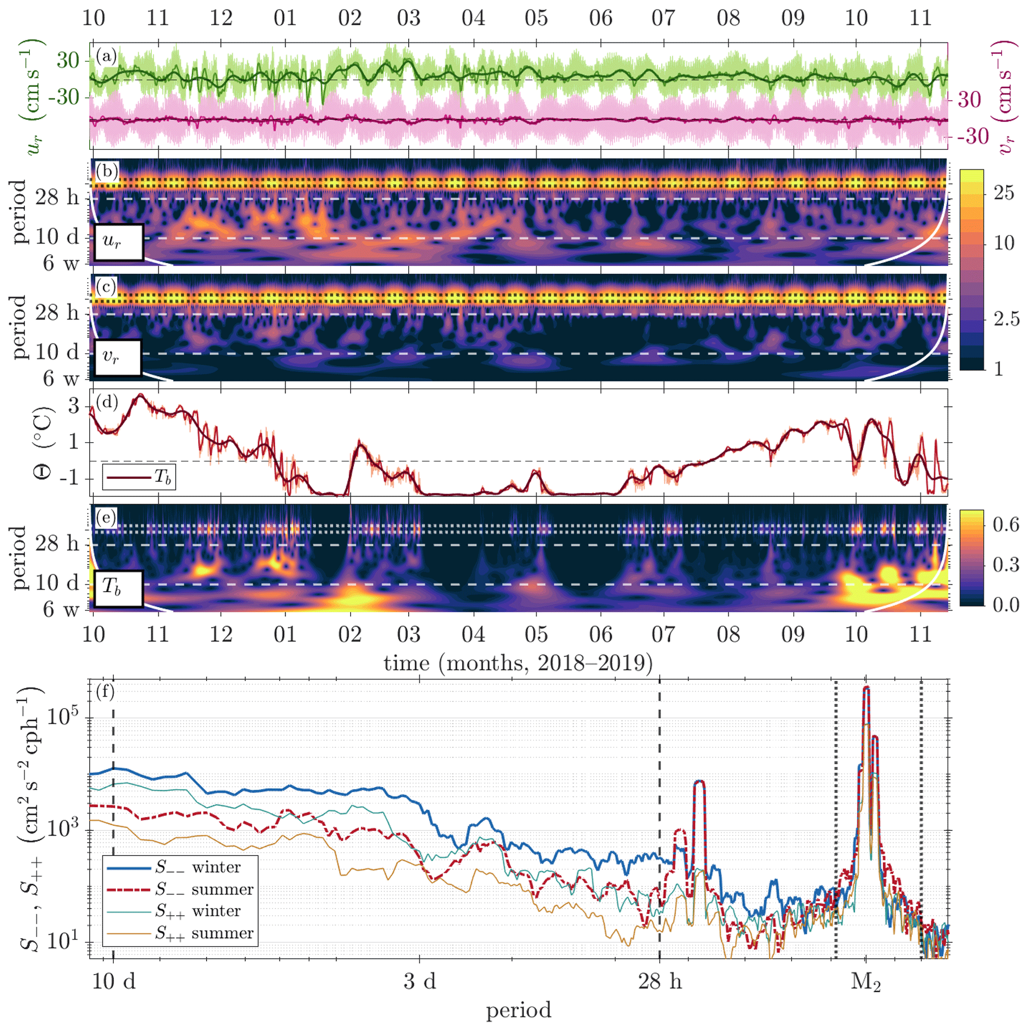
Figure 7 (a) Time series for the mooring deployment period (29 September 2018 to 14 November 2019) illustrating the depth-averaged velocity component along −28°, u_r (green; left y axis), and along 62°, v_r (pink; right y axis). The component is presented as measured (thin pale curves), low-pass-filtered over 28 h (thicker darker curves), and low-pass-filtered over 10 d (thickest darkest curves). (b, c) Wavelet transforms of u_r and v_r, respectively, shown on a logarithmic scale. Period corresponds to the inverse cyclic frequency, given in cycles per hour (cph). (d) Time series illustrating near-bottom temperature T_b with the same filtering as in panel (a). (e) Wavelet transform of T_b on a linear scale. (f) Rotary spectra (anticyclonic: thick curves; cyclonic: thin curves) of the depth-averaged current velocity for winter (October to March, blue and green curves) and summer (April to September; dashed red and yellow curves). The white curves in panels (b), (c), and (e) indicate areas affected by edge effects. The cutoff frequencies for the semidiurnal tidal band (dotted lines) and the weather band (dashed lines) are shown as horizontal lines in panels (b), (c), and (e) and as vertical lines in panel (f).

3.4 Mesoscale and tidal variability

A wavelet analysis of the current components u_r and v_r (along −28 and 62°, respectively) reveals a year-round dominance of semidiurnal tidal currents with a clear spring–neap cycle (Fig. 7a–c). The semidiurnal tidal current was anticyclonic (Fig. 7f), with variance oriented along 25°, i.e. nearly east-northeast (Sect. 3.6). When the near-bottom temperature T_b was above the freezing point, its semidiurnal variability typically ranged from 0.2 to 0.6 °C, occasionally reaching 0.8 °C.

Weather-band variability (28 h to 10 d) was considerable, particularly during the autumn months (November 2018 to January 2019) (Fig. 7b, c, and e), with the principal axis oriented along the WNW–ESE direction, approximately aligning with the topography, Sect. 3.6). T_b anomalies were typically within ±0.5 °C, but they doubled from November–December 2018 and from October–November 2019. At the beginning (October 2018) and towards the end of the record (October–November 2019), T_b exhibited elevated variance at the 10 d timescale; however, the edge effects of the wavelet analysis were significant (Fig. 7e).

The anticyclonic velocity component was generally more energetic than its cyclonic counterpart (Fig. 7f). The semidiurnal current exhibited almost 10 times more variance in the anticyclonic component, and the diurnal band showed almost all of its variance in the anticyclonic component. At lower frequencies, the currents were anticyclonic and elliptically polarised throughout the entire year (Fig. 7f), with the exception of winter, when the currents became nearly linearly polarised during periods of 2 weeks or more (not shown).

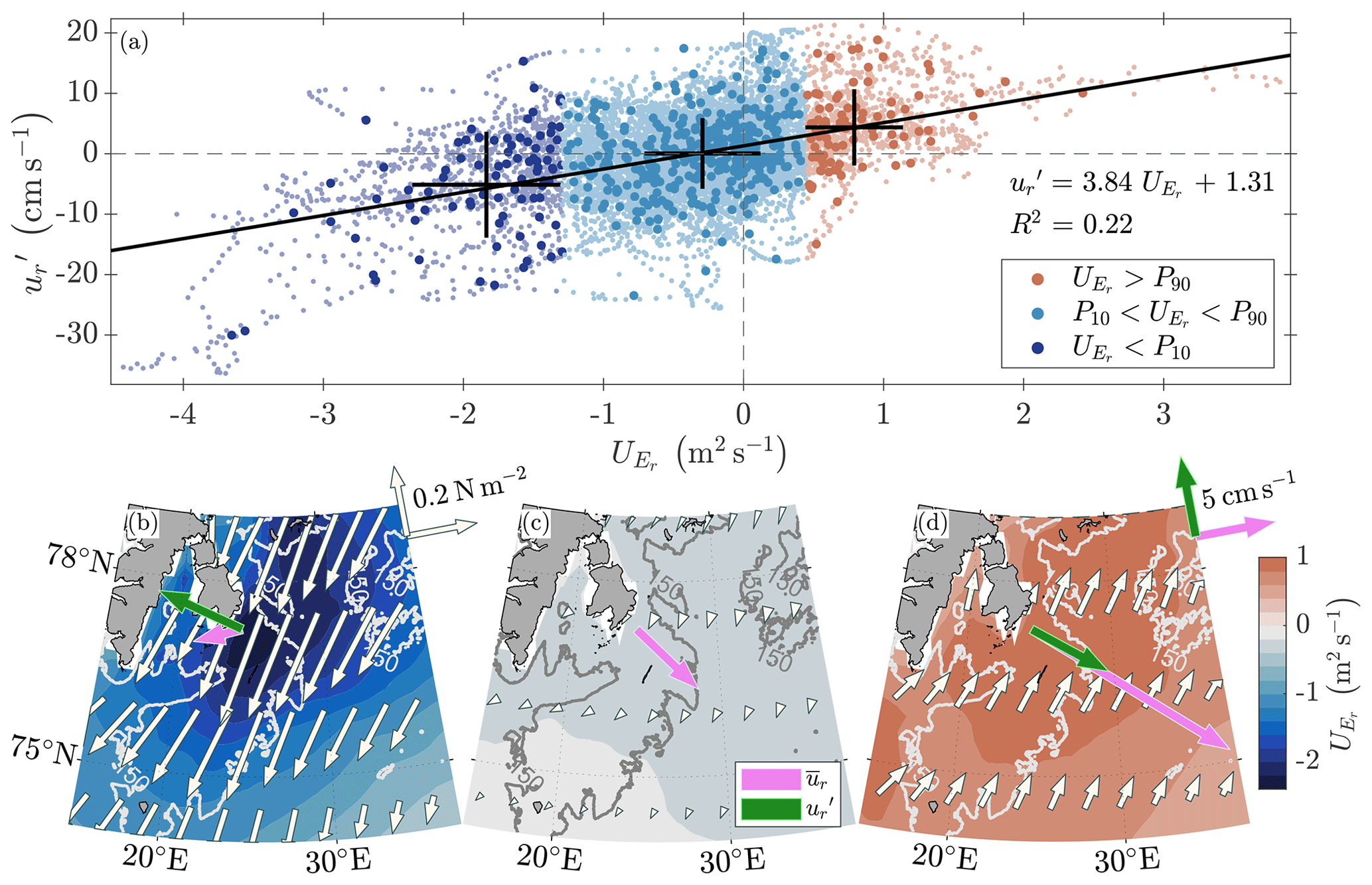
Figure 8 (a) Ekman transport, $U_{{\mathrm{E}}_{\mathrm{r}}}$ (m² s⁻¹), along −28° versus depth-averaged weather-band (28 h–10 d) current speed anomalies along −28°, ${u_{\mathrm{r}}}^{\prime }$. Colours indicate the $U_{{\mathrm{E}}_{\mathrm{r}}}$ composites: dark blue represents values below the 10th percentile, corresponding to strong north-northeasterly winds; light blue represents values between the 10th and 90th percentiles, corresponding to weak north-northeasterly winds; and orange represents values above the 90th percentile, corresponding to modest south-southwesterly winds. The small pale dots represent hourly values, while the larger dots represent daily averages. The current is lagged by 7 h relative to the wind before calculating $U_{{\mathrm{E}}_{\mathrm{r}}}$ and averaging it over time. The error bars show the mean and standard deviations of the daily averages within each composite. Maps illustrating composite averages of $U_{{\mathrm{E}}_{\mathrm{r}}}$ (coloured areas), wind stress (white quivers), the mean current (${\stackrel{\mathrm{‾}}{u}}_r$; pink quivers), and current anomalies (${u_{\mathrm{r}}}^{\prime }$; green quivers) for Ekman transport (b) below its 10th percentile, (c) between its 10th and 90th percentiles, and (d) above its 90th percentile. Reference quivers for wind stress (0.2 N m⁻²) and the current (5 cm s⁻¹) are shown in panels (b) and (d), respectively.

3.5 Impact of wind forcing on the across-saddle current

The strength and direction of the overflow current are influenced by large-scale winds (Fig. 8). Regression analysis shows that depth-averaged current anomalies along −28° in the frequency band ranging from 28 h to 10 d (${u_{\mathrm{r}}}^{\prime }$) depend on Ekman transport along the same axis. Geostrophic adjustment to Ekman transport during north-northeasterly winds typically opposes the east-southeastward current across the saddle (Fig. 8c) and, in cases of anomalously strong winds, even reverses it (Fig. 8b). Conversely, weaker and/or southerly winds tend to enhance the eastward flow into the Barents Sea (Fig. 8d).

Anomalously strong north-northeasterly winds, which result in Ekman transport values below the 10th percentile ($U_{{\mathrm{E}}_{\mathrm{r}}}=-\mathrm{1.84}(\pm \mathrm{0.53})$ m² s⁻¹ for daily averages), are associated with the strongest current reversal events (${u_{\mathrm{r}}}^{\prime }=-\mathrm{5.1}(\pm \mathrm{8.8})$ cm s⁻¹ for daily averages, with the current flowing towards the WNW along the topography) (Fig. 8b). The mean current velocity in this case is 3.1 cm s⁻¹, oriented towards the west-southwest, with a large spread.

On the other hand, winds with a southerly component, which result in Ekman transport values above the 90th percentile ($U_{{\mathrm{E}}_{\mathrm{r}}}=\mathrm{0.79}(\pm \mathrm{0.35})$ m² s⁻¹ for daily averages), are associated with the strongest east-southeastward currents (${u_{\mathrm{r}}}^{\prime }=\mathrm{4.4}(\pm \mathrm{6.3})$ cm s⁻¹ for daily averages) (Fig. 8d). This suggests that winds with a southerly component accelerate the normal east-southeastward current through geostrophic adjustment to the Ekman transport set-up. The average mean current in this case flows at 14.1 cm s⁻¹ towards the east-southeast.

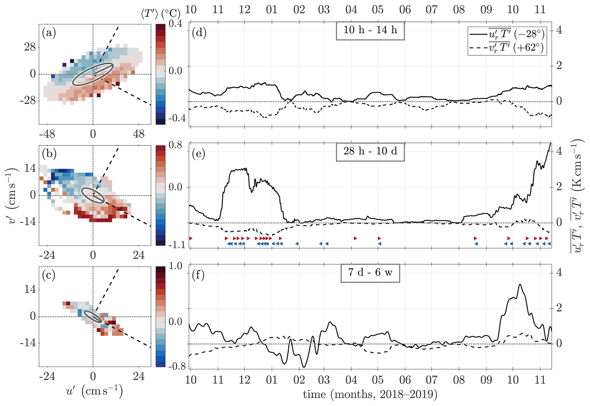
Figure 9 (a–c) Temperature anomalies (colours) averaged in bins of current velocity anomalies and examined with respect to the semidiurnal tidal band (a, d), weather band (28 h to 10 d; b, e), and lower-frequency band (7 d to 6 weeks; c, f). The velocity anomalies are layer-averaged over the bottom half of the water column, with their variance ellipses overlaid. (d–f) Time series illustrating eddy temperature flux along ($\stackrel{\mathrm{‾}}{{u_{\mathrm{r}}}^{\prime }{T}^{\prime }}$ (−28°); solid curves) and across ($\stackrel{\mathrm{‾}}{{v_{\mathrm{r}}}^{\prime }{T}^{\prime }}$ (62°); dashed curves) the principal axis of the weather band and variability in the lower-frequency band, which are shown in panels (b) and (c). The rotated coordinate system is indicated with dashed lines in the left column. Temporal averaging is performed using a 30 d running mean. Note that the u^′ and v^′ ranges for the semidiurnal band are twice as high as those for the other bands. In panel (e), the times of peaks chosen for ensemble averaging are marked with red triangles pointing right for positive temperature anomalies and along-isobath current anomalies and with blue triangles pointing left for negative anomalies.

3.6 Eastward transport of positive temperature anomalies

Variability in near-bottom temperature occurs in the same frequency bands as current variability (Fig. 7). We separated the contributions from tides, weather-band processes, and lower-frequency mesoscale activity by applying a band-pass filter to the time series of temperature and current velocity (Sect. 2.2). By analysing temperature anomalies T^′ in the velocity anomaly space $(u^{\prime },v^{\prime })$, we found that positive temperature anomalies were generally located in the southeastern sector of the velocity anomalies, while negative temperature anomalies were found in the northwestern sector, resulting in net heat transport directed southeastwards across the saddle in the identified bands of variability (Fig. 9a–c). For the weather and mesoscale-activity frequency bands (Fig. 9b and c, respectively), the largest temperature anomalies were aligned with the principal axis of variability (−28°). In the semidiurnal (Fig. 9a) and diurnal tidal bands (not shown), however, the largest temperature anomalies were nearly perpendicular to the axis of maximum variance (major axes of the ellipses).

The eddy temperature flux $\stackrel{\mathrm{‾}}{{u_{\mathrm{r}}}^{\prime }{T}^{\prime }}$ along the principal axis (−28°; solid curves in Fig. 9d–f) was generally positive throughout the year, with values typically between 1 and 2 K cm s⁻¹. The largest semidiurnal tidal contribution occurred from October to December in both years, with values around 1 K cm s⁻¹ directed towards the southeast. Comparable fluxes were also observed between February and July when warm, saline water intermittently appeared near the saddle. In the weather band, the flux was large from November 2018 to January 2019, with values ranging from 1 to 3 K cm s⁻¹, and again during the autumn of 2019, reaching 5 K cm s⁻¹ by the end of the measurement period (Fig. 9e). Between mid-January and August 2019, the flux was negligible. Lower-frequency oscillations on timescales between 1 and 6 weeks exhibited sporadic episodes of large positive eddy temperature fluxes during autumn and winter, reaching 3 K cm s⁻¹ in October 2019, but experienced reversals to negative values during January and February 2019 (Fig. 9f).

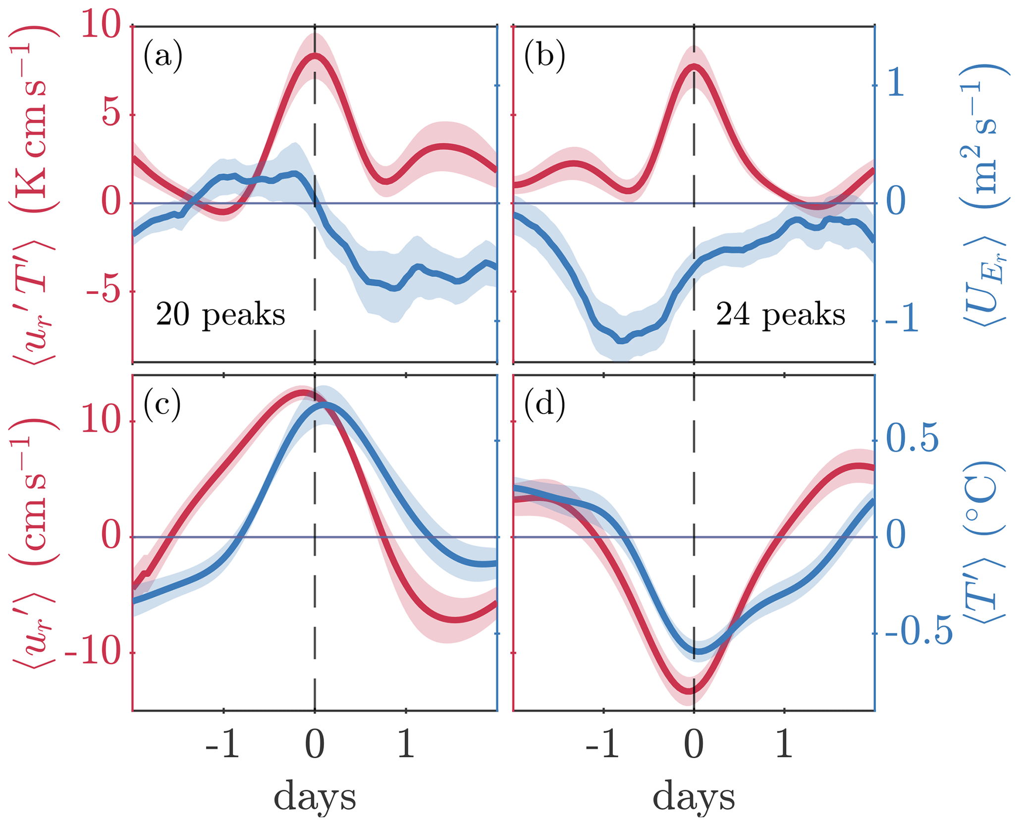
Figure 10 Ensemble-averaged time series illustrating events with strong positive eddy temperature flux $\langle u_{\mathrm{r}}^{\prime }{T}^{\prime }\rangle$ (red) along the direction of highest variance (−28°) in the weather band (28 h to 10 d). The time series show the cases where peaks $({u_{\mathrm{r}}}^{\prime },T^{\prime })>\mathrm{0}$ (i.e. positive temperature anomalies are carried ESE by the current anomaly along the isobath (a, c)) and where peaks $({u_{\mathrm{r}}}^{\prime },T^{\prime })<\mathrm{0}$ (i.e. negative temperature anomalies are carried WNW by the current anomaly along the isobath (b, d)). The ensemble time series include (a, b) $\langle u_{\mathrm{r}}^{\prime }{T}^{\prime }\rangle$ (red) and the Ekman transport component along −28°, $\langle U_{{\mathrm{E}}_{\mathrm{r}}}\rangle$ (blue), as well as (c, d) current anomalies $\langle {u_{\mathrm{r}}}^{\prime }\rangle$ (red) and temperature anomalies 〈T^′〉 (blue). The current anomalies are bin-averaged over the bottom half of the water column. The time axes (days) are centred on the peak of the eddy temperature flux. The standard error ($\mathrm{SE}=\mathrm{SD}\left(x\right)/\sqrt{n}$, where n is the number of ensembles) is indicated by shading.

To further investigate the driving force behind the eddy temperature flux across the saddle in the weather band, we analysed ensembles of events with high fluxes. In total 20 events with peaks $({u_{\mathrm{r}}}^{\prime },T^{\prime })>\mathrm{0}$ and 24 events with peaks $({u_{\mathrm{r}}}^{\prime },T^{\prime })<\mathrm{0}$ were detected, both resulting in positive eddy temperature fluxes. Most of these events occurred during October, November, and December (red and blue triangles in Fig. 9e), when there was no sea ice in the area. The 4 d time series, centred on the selected times for each event, were extracted. The ensemble-averaged records are denoted using angle brackets, e.g. 〈T^′〉 (Fig. 10).

The ensemble of events that satisfy the first condition is associated with southerly wind stress, resulting in an Ekman transport component that forces a positive current anomaly carrying positive temperature anomalies towards the east-southeast (Fig. 10a and c). The peak eddy temperature flux of $(\mathrm{8.4}\pm \mathrm{1.3})\mathrm{K}\mathrm{cm}{\mathrm{s}}^{-\mathrm{1}}$ tends to occur 1 d after the maximum along-isobath Ekman transport. The temperature anomaly turns positive approximately half a day after the current anomaly, and their peaks are 6 h apart.

The second case (Fig. 10b and d; events marked by blue triangles in Fig. 9e) corresponds to events where the wind from the north-northeast increases in strength, enhancing Ekman transport opposing the current. This results in a negative current anomaly that caries negative temperature anomalies towards the west-northwest. The peak of the eddy temperature flux reaches $\mathrm{7.8}(\pm \mathrm{1.2})\mathrm{K}\mathrm{cm}{\mathrm{s}}^{-\mathrm{1}}$ approximately 1 d after the along-isobath Ekman transport component has reached its largest negative value. The temperature anomaly turns negative 6 h after the current anomaly, and their peaks are 2 h apart.

4 Discussion

4.1 Interannual versus seasonal variability – was 2018–2019 a typical year?

Several findings from the time series at the mooring position (Fig. 6) and the late-autumn hydrographic transects at the saddle (Fig. 5) warrant a discussion about the seasonal and interannual variability in the area and whether 2018–2019 was a typical year.

The autumns of 2018 and 2019 differed in terms of hydrography and the onset of the sea ice period. During the autumn of 2018, the water column above the saddle remained warm and free of ice and was only partially covered with ice from December. In contrast, in the autumn of 2019, sea ice drifted to the saddle in late October, and the water cooled to near the freezing point in November. This suggests that the position of the ice cover in the Barents Sea during autumn affects the hydrographic conditions at the saddle at this time of the year. According to Kohlbach et al. (2023), the marginal ice zone had retreated beyond the shelf break and into the Nansen Basin by August 2018, while in August 2019, large parts of the northwestern Barents Sea shelf remained covered by sea ice, resulting in lower temperatures and a fresher surface layer. These differences in large-scale conditions at the end of the melting seasons in 2018 and 2019 must also have affected the subsequent winter conditions at our mooring site. During the same autumns, observations from the Northern Barents Sea Opening showed a large difference in upper-ocean salinity, accompanied by a similar difference in sea ice (Lundesgaard et al., 2022). Heightened upper-ocean freshening due to increased sea ice melt can create conditions in the area that are conducive to sea ice growth in the following winter (Lind et al., 2018).

Superposed on the seasonal cycle were several episodes of warm-water intrusions that affected sea ice cover at the saddle (Fig. 6b and c). The inflow of Atlantic-origin waters and heat transport across the saddle is important for the onset and duration of typical winter conditions. Strong current velocities directed across the saddle into the Barents Sea (u_R) generally preceded the local temperature maxima associated with the warm-water intrusions (Fig. 6c and d). Sea ice covered the mooring site from mid-January 2019, i.e. before the water column had completely cooled to the freezing point (Fig. 6b and c). Nonetheless, favourable wind and ice conditions, along with geostrophic adjustment to the wind-driven Ekman transport from Edgeøya to Hopen, resulted in depth-averaged currents reaching 23 cm s⁻¹, which drove warmer waters from the Storfjordrenna trough to the saddle. A similar response to wind forcing, resulting in deep warm-water overflow, has also been observed on the sill in the inner part of Hornsund in Svalbard (Arntsen et al., 2019).

However, not all warm-water inflow events can be explained by local wind effects. The event with a strong across-saddle current of 30 cm s⁻¹ and a small increase in temperature, which occurred from mid-February to March, was likely caused by upstream conditions. Accelerating the WSC and the branch entering the Storfjordrenna trough can force the current to follow shallower isobaths to conserve potential vorticity (Nilsen et al., 2016). The small increase in temperature during this period was most likely due to the mixing of warm water en route to the saddle. When the current subsided in early March, the temperature at the saddle returned to the freezing point, and the sea ice concentration increased to 90 %. Similarly, events during April involving weaker current pulses transporting cooler waters can be attributed to forcing resulting from the upstream conditions.

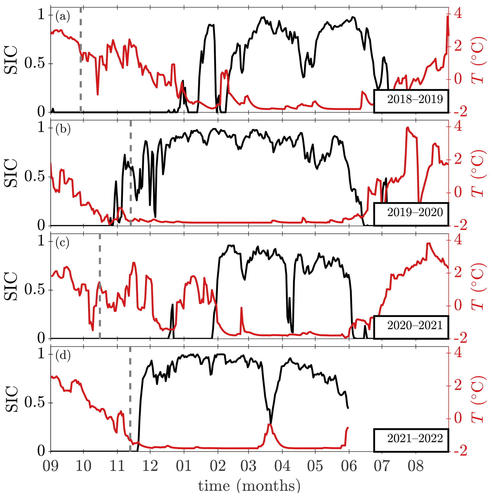
Figure 11 Sea ice concentration (black; left y axis) and sea surface temperature (red; right y axis) at the mooring location from (a) September 2018 to September 2019, (b) September 2019 to September 2020, (c) September 2020 to September 2021, and (d) September 2021 to September 2022. Dashed lines indicate the times of (a) mooring deployment, (b) mooring recovery and the hydrographic transect in November 2019, (c) the hydrographic transect in October 2020, and (d) the hydrographic transect in November 2021. Sea ice concentration and sea surface temperature are taken from the OSTIA product (OSTIA, 2023; Good et al., 2020).

Northeasterly winds and relatively strong westward-current reversals in the weeks preceding the November 2019 transect (Figs. 5a and 6a, d, and e) likely transported sea ice and cooled the surface waters above the saddle to the freezing point. Large-scale sea ice cover was more extensive in November 2019 than in November 2021. In 2019, the sea ice edge (characterised by 15 % sea ice concentration) extended past Hopen, almost reaching the southern tip of Spitsbergen, while in 2021, it only extended south to Edgeøya and did not cover the Olga Basin (not shown). The higher maximum temperature and the alignment of the isohalines and isotherms in the transect from November 2021 (Fig. 5c) suggest an autumn inflow of Atlantic-origin waters and incomplete cooling of the water column. The SST in the region was substantially higher in 2021 than in 2019, with the largest difference of 3 °C in the Storfjordrenna trough (not shown) and a difference of 1 to 2 °C at the mooring position. This meant that the onset of freezing was delayed by 1 month in 2021 relative to 2019 (Fig. 11b and d).

The November transects (Fig. 5a and c) were both cooler and less saline than the October transect (Fig. 5b). This may be due to a regular seasonal shift from AW influence to Arctic Water influence at the site and/or interannual variability in the region. During the autumn of 2020, SST steadily decreased before rapidly increasing to 1.4 °C in the week leading up to the transect in mid-October (Fig. 11c). It then decreased to 0 °C before increasing to 2.6 °C in mid-November. Hence, the autumn of 2020 experienced warmer and longer-lasting overflows of Atlantic-origin waters across the saddle and a delayed onset of sea ice compared to other years. AW inflow from north of Svalbard has also been shown to affect seasonal variability in local hydrography in the same way (Lundesgaard et al., 2022).

The autumn of 2018 was similar to the autumn of 2020 in terms of SST evolution at the mooring position (Fig. 11a and c). Warm-water inflow from the Storfjordrenna trough kept SST high at the saddle during November 2018 and November 2020, delaying the onset of sea ice in the subsequent winters.

In the context of long-term changes in SST and SIC at the study site, the period from the autumn of 2018 to the autumn of 2019 (mooring year) was an average year compared to the past 2 decades (not shown), and the difference between 2018 and 2019 was not remarkably large. From 2005, interannual variability in SST and SIC at the mooring site has been substantially higher than during the previous 25 years, indicating even larger year-to-year changes than those observed between 2018 and 2019 could be expected.

To summarise, strong interannual variability substantially impacts the seasonal cycle at the study site. Sea ice in the Barents Sea exhibits a high degree of interannual variability (e.g. Shi et al., 2024; Onarheim et al., 2024) driven by atmospheric temperature, sea surface temperature, and oceanic heat transport (Dörr et al., 2024). Locally, intrusions of warm water during autumn can delay the onset of winter conditions, inhibit local sea ice growth, or melt imported sea ice, as observed in the autumns of 2018 and 2020 (Figs. 6b–c, 5b, and 11a and c). These intrusions, whether driven by local winds or upstream conditions, also frequently reduce the existing partial ice cover above the saddle during winter and spring (Fig. 11; earlier years are not shown). This explains the differences in hydrographic conditions observed in November 2019 versus 2021 (Fig. 5a and c). The more persistent warm-water overflow in 2020 likely delayed the seasonal water mass transformation and contributed to the October 2020 transect being substantially warmer than the November transects.

4.2 Drivers of the mean exchange between the Storfjordrenna trough and the Barents Sea

The observed background current (low-pass-filtered over 10 d) tends to flow towards the southeast (Fig. 6c). This current direction is counteracted by geostrophic adjustment to Ekman transport induced by the large-scale wind pattern from the northeast. The strength and direction of the current are affected by the wind stress, and, in periods with strong winds, the current either reverses to a northwestward flow or is amplified in its normal southeastward direction (Fig. 8). Hence, local wind is not the main driver of the background current across the saddle.

The forcing of the slowly varying current is more complex. We found a low and insignificant correlation between spatial differences in sea level and mooring current velocity by analysing the absolute dynamic topography and the associated geostrophic currents (not shown). This means either that the local sea-level slope is not the main driver of the current or that the data coverage and quality of the measurements of the absolute dynamic topography are insufficient for showing a clear relationship. The quality of these measurements may be reduced as a result of seasonal ice coverage and the timing of satellite passages, and the quality of the product north of the Arctic circle has not been thoroughly tested (Oziel et al., 2020).

On the other hand, the current across the saddle may be dependent on the strength of the upstream current in the Storfjordrenna trough and along the slope west of Spitsbergenbanken (Sect. 4.1). Upstream, along the Norwegian coast, low-pressure systems accelerate the Norwegian Atlantic Current by driving onshore Ekman transport and set-up along the coast (Brown et al., 2023). However, it is unclear whether low-pressure systems would accelerate the WSC along the relatively shorter western Spitsbergen coastline (Brown et al., 2023). Additionally, high variability in the tracks of low-pressure systems passing Svalbard (Wickström et al., 2020) makes the influence of local wind west of the Storfjordrenna trough and Svalbard highly variable. Current peaks at the mooring site are occasionally related to a strong WSC, which can be quantified using the slope of the absolute dynamic topography between Spitsbergenbanken and the Storfjordrenna trough (not shown), contributing to the current strength in a barotropic manner. Similar to the response of the WSC on the West Spitsbergen Shelf to anomalous wind stress curl (Nilsen et al., 2016), the branch of the WSC flowing through the Storfjordrenna trough can be shifted to shallower isobaths. However, a more detailed analysis is needed to fully understand the effects of upstream forcing.

Another possible driver of the observed mean current is the tidal residual flow on Spitsbergenbanken. In shallow areas with strong tidal currents and non-linear bottom friction, residual currents may influence the circulation pattern (Harms, 1992). Tidally generated residual currents around Bjørnøya have been documented in buoy data (Vinje et al., 1989), laboratory experiments, and observations from drifters (McClimans and Nilsen, 1993). Several numerical model studies have shown that tidal rectification occurs in the region (Harms, 1992; Gjevik et al., 1994; Kowalik and Proshutinsky, 1995). Higher-resolution models which better resolve non-linear terms have reported strong anticyclonic residual tidal currents around Bjørnøya, on Spitsbergenbanken (reaching 15 cm s⁻¹), and around Hopen (Kowalik and Marchenko, 2023). Simulations have reproduced the anticyclonic drift of buoys around Hopen, which is driven by strong tidal currents resulting from the interaction between the semidiurnal tide and the island of Hopen (Marchenko and Kowalik, 2023).

4.3 Variability in tidal, weather, and low-frequency bands and its impact on eastward heat transport into the Olga Basin

Both semidiurnal and diurnal tidal currents contribute to heat transport across the saddle on Hopenbanken, with the semidiurnal contribution being significantly larger. The semi-major axis of the semidiurnal currents is oriented along 20°, i.e. roughly east-northeast, which is approximately perpendicular to the eddy temperature flux in the semidiurnal band (Fig. 9). For all frequency bands, the direction of the eddy temperature flux is mainly oriented towards the southeastern sector. This is likely due to the position of the temperature gradient at the saddle and the way the current anomalies are guided by the topography.

Oscillations on timescales between 1 and 6 weeks result in sporadic moderate eddy temperature fluxes in the southeastern sector, comparable in magnitude to those in the semidiurnal band but more variable in direction. The largest contribution towards the east-southeast occurred during the autumn of 2019 (Fig. 9f), when the wavelet transform of u_r (Fig. 7b), and especially that of T_b (Fig. 7e), exhibited power in the low-frequency area, indicating that the varying current resulted in even larger temperature variations. These concurrent fluctuations led to a considerable eddy temperature flux during this period. We hypothesise that the large eddy temperature flux during this autumn may have been caused by AW upstream of the saddle being transported across shallower isobaths, possibly due to regional Ekman pumping or an acceleration of the upstream current system, which resulted in higher temperatures on one side of the front at the saddle. Locally, at the mooring site, this was observed as low-frequency oscillations with particularly pronounced temperature variations, leading to a large eddy temperature flux into the Barents Sea.

Integrated over the measurement period, the weather-band eddy temperature flux was approximately twice that of the low-frequency and semidiurnal bands, which had comparable magnitudes. During the period of relatively high sea ice coverage (from February to July), the semidiurnal tide transported twice as much heat across the saddle as the weather band and 1.5 times as much as the band associated with mesoscale activity.

The eddy temperature fluxes calculated in Sect. 3.6 contain divergent and rotational components. Only the divergent component plays a part in the actual transport of heat across the saddle (Marshall and Shutts, 1981; Guo et al., 2014). Using our data set, we cannot separate the contributions of the divergent and rotational eddy temperature fluxes; hence, the values must be considered an upper bound.

4.4 Consequences of long-term changes in the hydrographic environment of the Storfjordrenna trough for heat transport into the Barents Sea

In recent years, the presence of AW in the Storfjordrenna trough upstream of the study site has increased. The Storfjordrenna trough is one of the areas in the Barents Sea that has experienced the highest increase in sea surface temperature over the past 2 decades (Barton et al., 2018; Mohamed et al., 2022b). The climatology in the Storfjordrenna trough (Sect. 3.1) also shows that the water column has become warmer since 2000 compared to previous years (Fig. 3) and that Atlantic-origin waters have shoaled and now reach further east towards the saddle during summer (Fig. 4). Shoaling has also been observed in the Eurasian Arctic (Polyakov et al., 2017) as well as along the coast and in the fjords of western Spitsbergen (Tverberg et al., 2019; Skogseth et al., 2020; Strzelewicz et al., 2022). Additionally, AW advected into the fjords of western Spitsbergen has warmed in the past 2 decades (Bloshkina et al., 2021; Pavlov et al., 2013; Tverberg et al., 2019; Skogseth et al., 2020). At the mooring site, the years following 2005–2006 saw, on average, higher mean annual SSTs and fewer days of sea ice coverage compared to the years between 1981–1982 and 2004–2005 (not shown), which may be due to increased AW inflows into the Barents Sea after 2006 compared to the Fram Strait (Polyakov et al., 2023). The warmest year in this period was 2015–2016, which saw abnormally high mean SSTs over the saddle, only 106 d with any sea ice, and no SIC value above 80 %. This was also the year when the Storfjordrenna trough, along with the Barents Sea in general (Mohamed et al., 2022b), experienced record-low sea ice cover, a warm saline surface layer (Vivier et al., 2023), and an exceptionally warm and long-lasting marine heatwave (Mohamed et al., 2022a).

As AW circulates over shallower isobaths, the physical processes in the channel between the Storfjordrenna trough and the Olga Basin may more easily transport heat eastwards in the future. Anomalous wind stress curl may affect the circulation depth of AW in the Storfjordrenna trough, potentially causing AW or Atlantic-origin waters to move closer to the saddle between the Storfjordrenna trough and the Olga Basin (Sect. 4.2).

Several factors determine the fate of warm waters crossing the saddle. The circulation pattern in the channel and downstream influences whether Atlantic-origin waters are transported towards the Arctic or the Atlantic side of the polar front, which follows the 200 m isobath separating the Olga Basin from Hopendjupet (Fig. 2). Although the time-averaged flow observed by the mooring was directed towards the southeast, with most non-tidal variability contributing to heat exchange along the west-northwest–east-southeast axis (Sect. 3.4, 3.5, and 3.6), the region's complex bathymetry and limitations in our observations prevent a definitive conclusion regarding the specific path of AW and the proportion of heat contributing to the heat budget on the northern side of the polar front. Nonetheless, AW transport through the channel between the Storfjordrenna trough and the Olga Basin has the potential to impact the Olga Basin, which still experiences a seasonal ice cover and maintains a thick cold layer of Arctic Water (e.g. Lind and Ingvaldsen, 2012).

Given the possibility that Atlantic-origin waters from the Storfjordrenna trough may be transported to the Arctic side of the polar front east of Hopenbanken, the density stratification within the Olga Basin becomes an important factor in determining the impact of this transport on local conditions. Denser waters on the eastern side would cause Atlantic-origin waters to penetrate at shallower depths, impacting the winter and spring sea ice cover and generally depositing more heat into the upper part of the water column, which could influence sea ice growth in the subsequent season. Conversely, less dense waters on the eastern side might lead to the subduction of overflow waters. If pure AW, or water with properties more similar to those of AW than those observed in this study, flows over the saddle, its density may exceed that of local water in the Olga Basin (e.g. Arctic Water and East Spitsbergen Water) and thus contribute to deeper stratification. We observed a deepening of the 34.4 g kg⁻¹ isobath and a small decrease in temperature in parts of the Olga Basin (Fig. 4b and c) over the past 2 decades. However, due to the particularly sparse data coverage in the Olga Basin, we are cautious about interpreting these changes.

Atlantic-origin waters reaching the saddle between the Storfjordrenna trough and the Barents Sea will affect the properties of the East Spitsbergen Current as it flows into Storfjorden. An increase in AW mixed into the East Spitsbergen Current across the saddle will have repercussions for the coastal current in Storfjorden and along the west coast of Spitsbergen, as well as for the exchange between the shelf and the fjords. It will also affect dense-water production in Storfjorden and subsequent deep-water export to the Fram Strait, as the initial salinity of the source water sets the conditions for the density of the overflow (Schauer, 1995; Skogseth et al., 2004; Vivier et al., 2023).

5 Conclusions

We have used available historical hydrographic profiles to study changes in the hydrographic environment of the Storfjordrenna trough, the surrounding shallow banks, and the Olga Basin (north of the polar front) over the past 2 decades, comparing this period to 1930–2000. In addition, we analysed recent late-autumn hydrographic transects and a year-long time series of near-bottom hydrography and water column current velocity across the saddle that separates the Storfjordrenna trough from the Olga Basin, situated between the islands of Edgeøya and Hopen.

The mooring observations show that AW and Atlantic-origin waters in the Storfjordrenna trough can cross the saddle and enter the Arctic domain of the northwestern Barents Sea. The across-saddle current is mediated by wind forcing. Southerly winds over the saddle cause stronger currents to flow into the Barents Sea and are associated with events demonstrating strong eddy temperature fluxes. The pronounced semidiurnal tidal currents over the saddle also contribute to heat transport into the Barents Sea, accounting for about half of the wind-driven flux. The area is characterised by large seasonal and interannual variability in hydrography and sea ice cover as well as frequent intrusions of warm water from the Storfjordrenna trough. Both local wind stress and upstream conditions can drive these intrusions, and they are important for determining the onset and duration of typical winter conditions in the area.

The past 2 decades has experienced higher temperatures and an increased influence of AW in the Atlantic sector of the northwestern Barents Sea. This increase in heat in the Atlantic sector, combined with potential shoaling of AW and ongoing changes in large-scale wind patterns, indicates that the channel separating the Storfjordrenna trough from the Barents Sea may emerge as an important pathway enabling AW and heat to enter the Arctic sector of the Barents Sea in the future. The complex interplay of local and non-local processes that drive the large variability in AW inflow on seasonal to interannual timescales highlights the need for more comprehensive data collection and analysis in this area.

Appendix A: Methodology for the climatological hydrography maps and sections

The historical hydrographic data were optimally interpolated onto horizontal and vertical climatological sections to compare the past 2 decades with earlier decades. The interpolation was conducted using the kriging algorithm from Surfer 12 (Golden Software) through the MATLAB function “surfergriddata.m”. This method employed point kriging with no drift, utilising a linear variogram model with unit slope and anisotropy. The spatial resolution of the bin averages prior to kriging is described in Sect. 4.2 and 4.3 of Skogseth et al. (2020). Due to the temporally and spatially sparse data coverage, only summer (July–October mean) sections could be created. For the period 1930–2000, bins with data from fewer than 3 years were retained without data to ensure an unbiased representation. For the period 2000–2019, this minimum threshold was lowered to 1 year to ensure sufficient data for producing the kriging-interpolated sections. Data coverage and standard deviations for the horizontal climatological sections are shown in Figs. A2 and A1, while those for the vertical climatological sections are shown in Figs. A4 and A3.

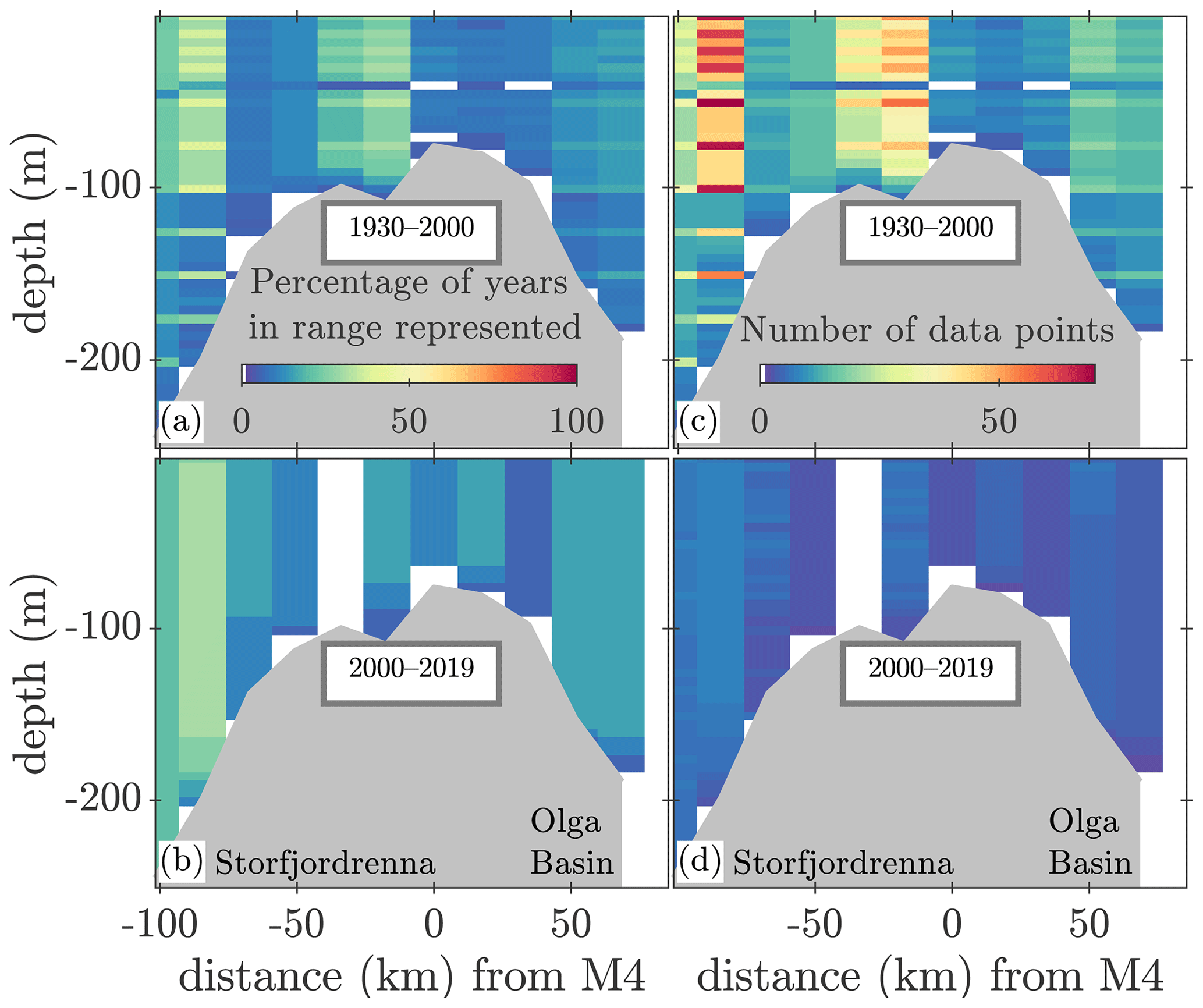
Vertical climatological sections corresponding to summertime (July–October) temperature and salinity over the periods 1930–2000 and 2000–2019 were constructed from hydrographic profiles within a ± 0.15° perpendicular distance from a section extending from the Storfjordrenna trough, across the saddle, and into the Olga Basin. This section comprises the bin centres shown in Fig. 3a. The bin sizes in the along-section direction were half the distance between two neighbouring bin centres. At the endpoints of the sections, profiles within 0.3° west (east) of the western (eastern) bin centre were included in the bin average. Each profile was weighted based on its distance to the bin centre to produce weighted bin-averaged sections with a 5 m vertical resolution. The weighted bin-averaged sections were then interpolated onto a 500 m (horizontal) × 5 m (vertical) grid resolution using kriging interpolation.

Similarly, weighted bin-averaged horizontal distributions of depth-averaged temperature and salinity over the entire water column were estimated using a 0.5° (longitude) × 0.2° (latitude) grid resolution for the region between 76–78° N and 20–28° E. Here, each profile was weighted according to its distance from its corresponding bin centre. The weighted bin-averaged horizontal sections for depth-averaged temperature and salinity were then interpolated onto a grid with double the resolution using the kriging interpolation method described above. Land points were excluded from both grids.

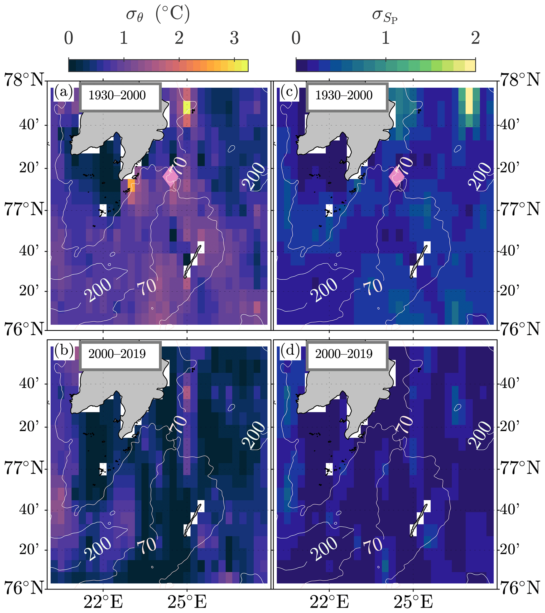
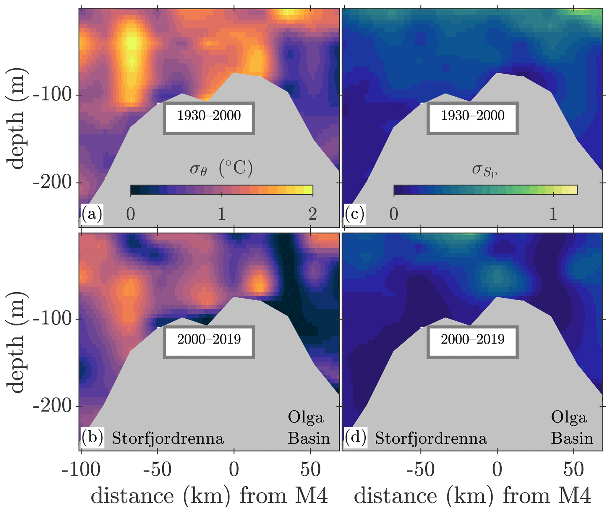
Figure A1 Standard deviations of (a, b) potential temperature σ_θ (°C) and (c, d) practical salinity ${\mathit{\sigma }}_{S_{\mathrm{P}}}$ for the periods (a, c) 1930–2000 and (b, d) 2000–2019 with respect to the depth-averaged horizontal climatological hydrographic maps (Fig. 3). The 70 and 200 m isobaths are indicated by white contours. The mooring location is indicated by a pink diamond.

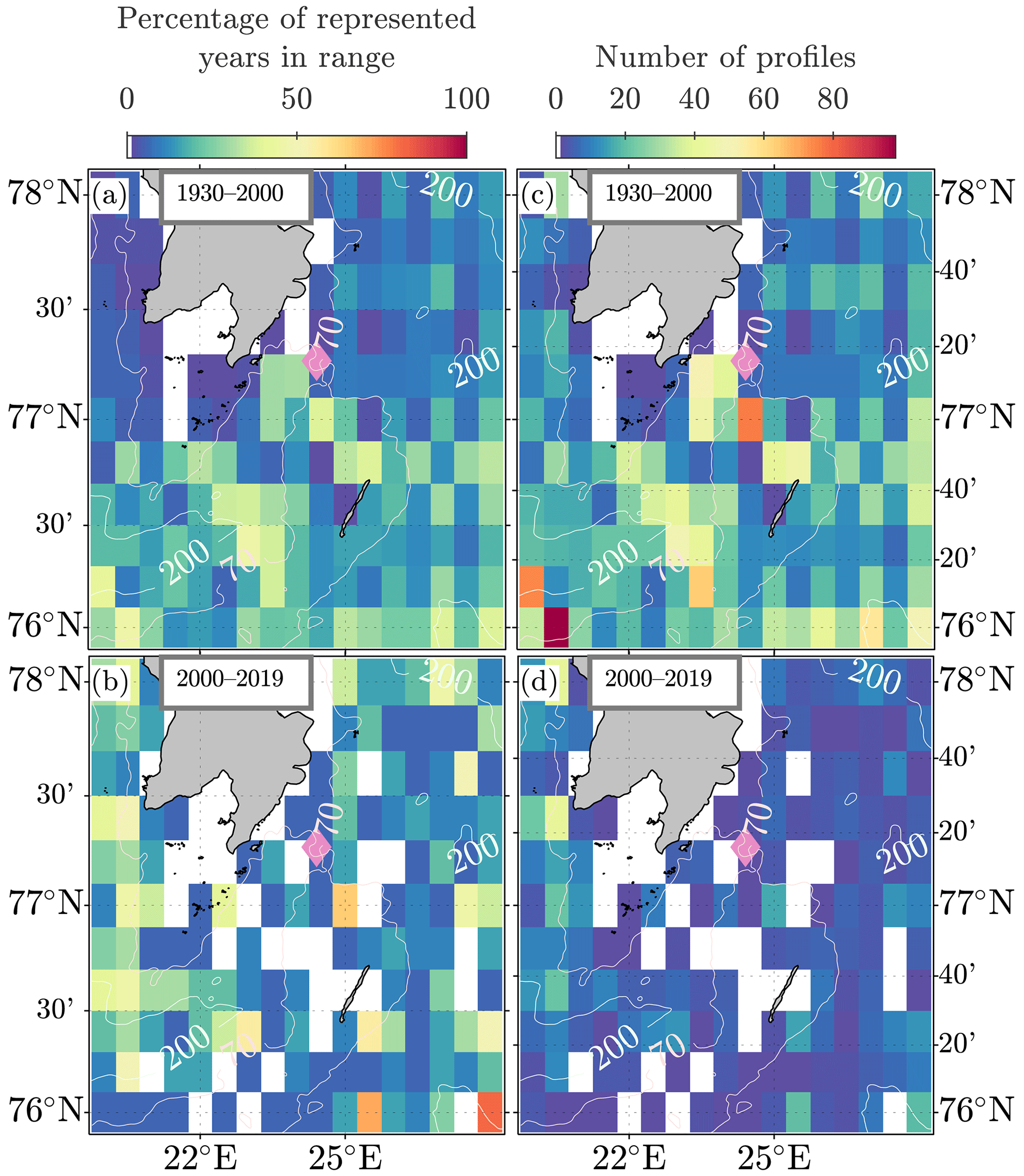
Figure A2 Data coverage corresponding to (a, b) the percentage of years with at least one profile and (c, d) the number of profiles for (a, c) 1930–2000 and (b, d) 2000–2019 with respect to the depth-averaged horizontal climatological hydrographic maps (Fig. 3). The 70 and 200 m isobaths are indicated by white contours. The mooring location is indicated by a pink diamond.

Figure A3 Same as Fig. A1 but with regard to the vertical climatological hydrographic transects (Fig. 4). The x axis shows the distance to the mooring position, with positive values indicating the direction towards the Olga Basin. The location of the section is indicated by green dots in Fig. 3a.

Figure A4 Same as Fig. A2 but with regard to the vertical climatological hydrographic transects (Fig. 4). The x axis shows the distance to the mooring position, with positive values indicating the direction towards the Olga Basin. The location of the section is indicated by green dots in Fig. 3a.