the Creative Commons Attribution 4.0 License.
the Creative Commons Attribution 4.0 License.
 | 11 Jul 2024
The Polar Front in the northwestern Barents Sea: structure, variability and mixing
Eivind H. Kolås
Ilker Fer
Till M. Baumann
In the northwestern Barents Sea the warm and salty Atlantic Water meets the cold and fresh Polar Water, forming a distinct thermohaline front, the Barents Sea Polar Front. Here we present the structure of the front, its variability and associated mixing using observations from two cruises conducted in October 2020 and February 2021 during the Nansen Legacy project in the region between the Hopen Trench and the Olga Basin. Ocean stratification, currents and turbulence data were obtained during seven ship transects across the Polar Front near 77° N, 30° E. These transects are complemented by four missions using ocean gliders, one of which was equipped with microstructure sensors to measure turbulence. Across the front, we observe warm (> 1 °C) and salty (> 35.0 g kg−1) Atlantic Water intruding below the colder (< 0 °C) and fresher (< 34.6 g kg−1) Polar Water, setting up a baroclinic front and geostrophic currents reaching 25 cm s−1, with estimated eastward transport of 0.2±0.6 Sv (1 Sv m3 s−1). We observe anomalous warm- and cold-water patches on the cold and warm side of the front, respectively, colocated with enhanced turbulence, where dissipation rates of turbulent kinetic energy range between 10−8 and 10−7 W kg−1. Short-term variability below the surface mixed layer arises from tidal currents and mesoscale eddies. While the effects of tidal currents are mainly confined to the bottom boundary layer, eddies induce significant shifts in the position of the front and alter the isopycnal slopes and the available potential energy of the front. Substantial water mass transformation is observed across the front, likely a result of eddy-driven isopycnal mixing. Despite the seasonal changes in the upper layers of the front (0–100 m) influenced by atmospheric forcing, sea ice formation and brine rejection, the position of the front beneath 100 m depth remained relatively unperturbed.
- Article
(12634 KB) - Full-text XML
- BibTeX
- EndNote


The Barents Sea is one of the main gateways through which Atlantic Water (AW) enters the Arctic Ocean (Fig. 1). About 2 Sv (1 Sv = 1×10⁶ m3 s−1) of AW enters through the Barents Sea Opening (BSO) in the west, continuing as a topographically steered current along the Bear Island Trough (Loeng, 1991; Smedsrud et al., 2010). Upon reaching the Central Bank, about 1 Sv of AW continues north along the Hopen Trench towards the Great Bank (Kolås, 2024, Chap. 4). Polar Water (PW) enters from the north, occupying most of the Great Bank and the Spitsbergen Bank (Loeng, 1991; Lien et al., 2017). The location where these two water masses meet is named the Barents Sea Polar Front (Loeng, 1991; Harris et al., 1998; Oziel et al., 2016) and is a site for water mass transformation with significance for both the overturning circulation and the ventilation of the Arctic Ocean (Årthun et al., 2011). Water masses are defined in Sect. 3.1, Table 3.
The Barents Sea Polar Front, which we refer to as the Polar Front (PF), is part of the North Polar Frontal Zone, a major climatic feature in the Nordic Seas where the characteristic scale of temperature and salinity variability is 5–50 km (Rodionov, 1992). The frontal zones are highly dynamical regions with mesoscale features ranging from a few to hundreds of kilometers, including, but not limited to, fine structures due to local wind, precipitation, internal waves, isolated eddies, frontal meanders and advective intrusions (Rodionov, 1992; Gula et al., 2022).
The PF is mainly topographically steered, particularly in the western Barents Sea from Bear Island along the Spitsbergen Bank to the Great Bank (for place names see Fig. 1), where it follows the 200–250 m isobath (Johannessen and Foster, 1978; Gawarkiewicz and Plueddemann, 1995;
Oziel et al., 2016; Kolås et al., 2024). However, the climate of the Barents Sea has been shown to affect the position of the front south of Bear Island; in warmer periods with stronger winds, the front shifted upslope compared to colder periods (Ingvaldsen, 2005). Around the Central Bank and in the eastern Barents Sea, the PF is not as stationary as it is along the Spitsbergen Bank, covering a broader zone of mixing (Oziel et al., 2016).
There have been few detailed studies of the frontal structure in the Barents Sea. The Barents Sea Polar Front Experiment studied the front at the southern flank of the Spitsbergen Bank in summer 1992 (Gawarkiewicz and Plueddemann, 1995; Parsons et al., 1996). The upper 20–40 m of the PF is characterized by a clear horizontal salinity gradient separating Arctic meltwater in the north from Atlantic surface water in the south. Because the horizontal temperature gradient is weak in the surface mixed layer, the surface front manifests as a density front, with a maximum density difference across the front of about 0.8 kg m−3 (Parsons et al., 1996). Between the surface layer and 100 m depth, the front is defined by a horizontal temperature gradient and contains numerous fine-structure intrusions (Parsons et al., 1996). Below 100 m from the surface, the gradients are weaker, likely due to bottom boundary mixing (Fer and Drinkwater, 2014), resulting in a broader frontal zone. In addition, the horizontal temperature and salinity gradients below 100 m depth compensate for their contribution to density, resulting in a barotropic front with horizontal density lines (Gawarkiewicz and Plueddemann, 1995; Parsons et al., 1996). While other observations such as those by Johannessen and Foster (1978), Fer and Drinkwater (2014) and Våge et al. (2014) agree on the overall structure of the PF, the circulation and interaction of AW and PW across the front remain poorly understood.

Figure 1(a) Overview map of the Barents Sea. The gray contour indicates the 200 m isobath. Red arrows outline the main Atlantic Water pathways. The dashed black line shows the Barents Sea Opening (BSO). (b, c) Zoom-in on the northwestern Barents Sea at the time of the fall and winter cruise, respectively, showing sea surface temperature (SST) and sea ice concentration (SIC). The black line indicates the sea ice edge where the SIC is 15 %. Isobaths are drawn at 200 and 350 m depth. Yellow rectangles show the frontal region studied. The white line in panel (c) indicates the 0 °C isotherm in the SST data. The SIC is from EUMETSAT OSI-SAF (2017). The SST is from the product SEAICE_ARC_SEAICE_L4_NRT_OBSERVATIONS_011_008 from Copernicus (2019). (d) The SST and SIC spatially averaged over the yellow box in panel (b). (e) Daily mean winds at 10 m height (W10) spatially averaged over the yellow box in panel (b) and smoothed over 7 d. Glider and cruise periods are highlighted in red and blue, respectively (SG: Seaglider; GOS: R/V G.O. Sars; KH: R/V Kronprins Haakon).
Direct measurements of turbulent mixing along the PF suggest that diapycnal mixing is mainly confined to the boundary layers during strong tidal currents and/or strong-wind events (Sundfjord et al., 2007; Fer and Drinkwater, 2014). Using detailed measurements of ocean turbulence, hydrography, currents and nutrients from the PF across Spitsbergen Bank near Hopen in May 2008, Fer and Drinkwater (2014) observed enhanced biological activity between a density-compensated thermohaline front near the 150 m isobath and a tidal front on the cold side of the PF. Tidal currents along the slope of the Spitsbergen Bank can have a peak-to-peak variability of 1 m s−1, and bottom boundary dissipation rates reach 10−6 W kg−1 (Fer and Drinkwater, 2014). However, on the warm side of the PF, away from the boundary layers, waters are in general quiescent, and mixing mainly occurs along isopycnals with interleaving layers of AW and PW (Fer and Drinkwater, 2014; Våge et al., 2014). Using concomitant measurements of turbulence and biogeochemical variables collected during the same October 2020 cruise reported here, Koenig et al. (2023) estimated a substantial transfer of nitrate and dissolved inorganic carbon across the PF from the Atlantic domain to the Arctic domain. Vertical fluxes driven by Ekman pumping were of a similar magnitude as the vertical turbulent fluxes.
Another source for mixing along the front can be mesoscale eddies. Eddies detaching from a mean flow diffuse properties along isopycnal surfaces, redistributing heat, salt and nutrients (Mcwilliams, 2008). Eddies are known to play a key role in distributing AW heat in the Arctic Ocean (von Appen et al., 2022), particularly along the AW inflow west and north of Svalbard (von Appen et al., 2016; Hattermann et al., 2016; Crews et al., 2018; Våge et al., 2016). In the Barents Sea, satellite radar images from 2007 and 2011 indicated that eddies were frequently generated near the PF southwest of Svalbard (Atadzhanova et al., 2018). However, the role of these eddies in distributing and mixing AW in the Barents Sea is not clear. Porter et al. (2020) observed a cold-core surface eddy south of the PF in the Hopen Trench and traced its origin back to the north of the PF using sea surface height from satellites. Combining their observations with those of Atadzhanova et al. (2018), they estimated that the southward transport of cold and fresh water by eddies forming in the PF region was about 0.35 Sv. In addition, Porter et al. (2020) state that this transport is likely an underestimate as eddies in the Barents Sea PF region tend to be masked from satellite-derived sea surface temperature (SST) observations due to thermal capping. The role of eddy-driven along-isopycnal mixing of AW across the PF in the Barents Sea requires further investigation.
The purpose of this paper is to describe the hydrography, dynamics and mixing in the vicinity of the PF, using observations from multiple repeat transects over different timescales from tidal cycle to seasons. The dataset coverage is a significant advance relative to earlier studies. The specific location studied is the sill between the Hopen Trench and the Olga Basin (yellow square, Fig. 1b). This region is of particular interest, as the AW flowing north towards this sill is able to cross below the PF and continue northwards as a topographically steered current (Kolås, 2024, Chap. 4).
Observational data from two scientific cruises in fall 2020 and winter 2021 (Fer et al., 2023e, b, c, d, a) are supplemented by four glider missions (Kolås et al., 2022) covering the Barents Sea Polar Front in the period from 2019 to 2021. An overview of the data and the corresponding source to access the data are listed in Table 1. All data were collected as part of the Nansen Legacy project. The data presented here are a subset of a larger dataset reported in Kolås et al. (2024, preprint), which addressed the AW circulation and hydrography in the northwestern Barents Sea and compared it to historical data. An overview of the data coverage across and near the front is shown in Fig. 2. Platform-specific details are given in the following subsections.
Kolås et al. (2022)Kolås et al. (2022)Fer et al. (2023a)Fer et al. (2023e)Kolås et al. (2022)Fer et al. (2023c)Kolås et al. (2022)Fer et al. (2023d)Fer et al. (2023b)Table 1Overview of data used in this study. See text for platform, instrument and sensor descriptions.

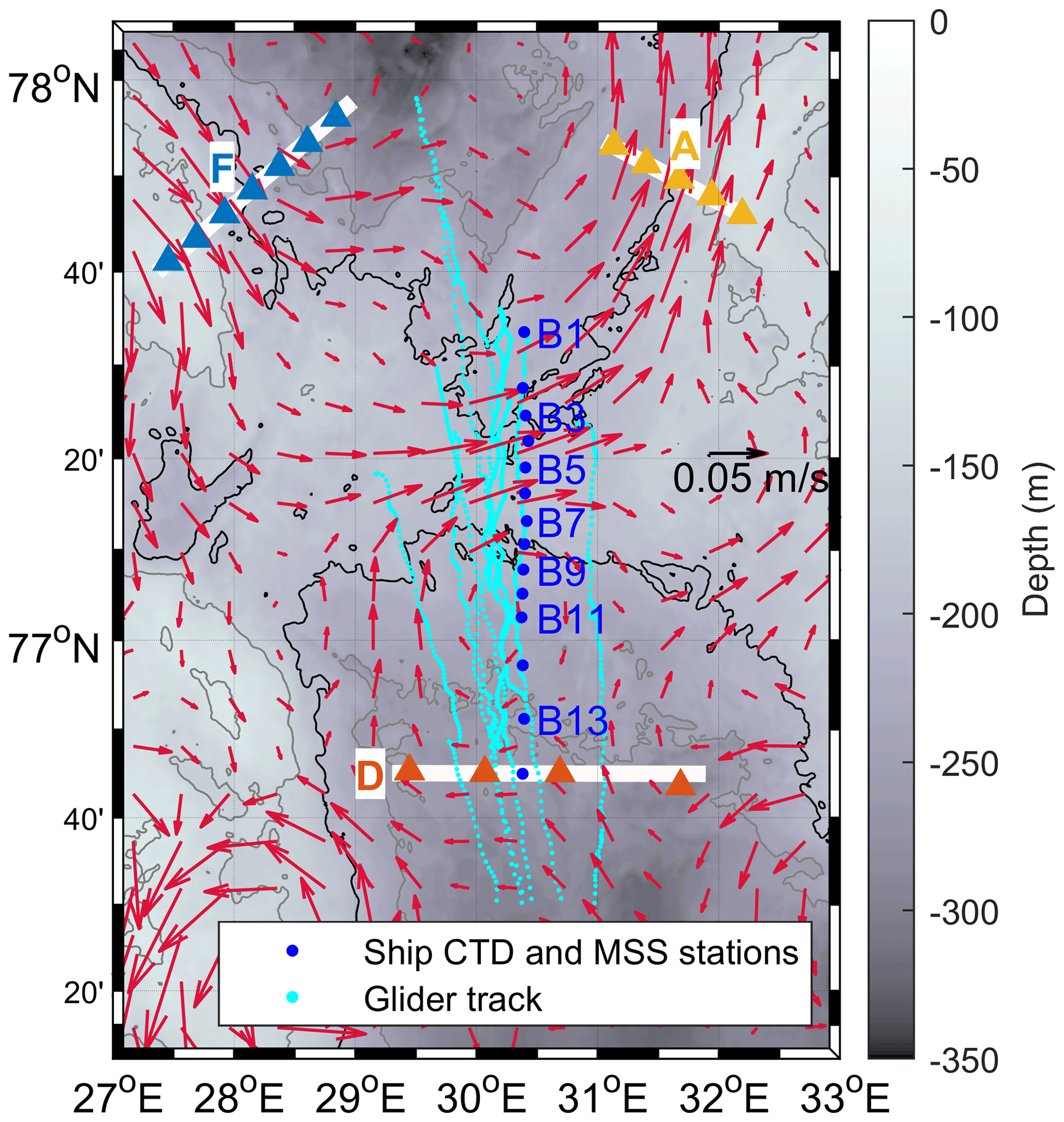
Figure 2Overview of the data coverage across the PF on the sill between the Hopen Trench (south) and the Olga Basin (north). Isobaths are shown at every 50 m between 50 and 300 m, and the 200 m isobath is highlighted in black. Red quivers are a subset of the objectively mapped, divergence-free, depth-averaged currents presented in Kolås et al. (2024, preprint). The black quiver shows the scale. White sections (A, D and F) with adjoining triangles show the locations of the CTD profiles presented in Fig. 9.
2.1 Hydrographic measurements from cruises
The cruises were conducted on board the Research Vessel (R/V) G.O. Sars between 6 and 27 October 2020 (cruise report: Fer et al., 2021) and the icebreaker R/V Kronprins Haakon between 9 February and 1 March 2021 (cruise report: Nilsen et al., 2021). We will call them the fall cruise and the winter cruise, respectively. Conductivity–temperature–depth (CTD) profiles during both cruises were collected using a Sea-Bird Scientific SBE 911plus CTD system, with a 200 kHz Benthos altimeter allowing measurements close to the seabed. The CTD system was equipped with an SBE 32 Carousel fitted with bottles for collecting water samples at all stations. Bottle samples were analyzed using a Guildline Portasal 8410 salinometer and used to calibrate salinity. A total of 64 and 89 CTD profiles were collected during the fall and winter cruises, respectively. Pressure, temperature and practical salinity data are accurate to ±0.5 dbar, °C and , respectively. CTD data were processed using the standard SBE Data Processing software. Conservative Temperature, Θ, and Absolute Salinity, SA, were calculated using the thermodynamic equation of seawater (IOC et al., 2010) and the Gibbs-SeaWater Oceanographic Toolbox (McDougall and Barker, 2011). Cruise CTD data are accessible from Fer et al. (2023a) and Fer et al. (2023d).
2.2 Current profiles from cruises
The CTD frames on both vessels were fitted with a pair of acoustic Doppler current profilers (ADCPs), so-called lowered ADCPs (LADCPs). The LADCPs were 300 kHz Teledyne RD Instruments (RDI) Workhorse Sentinels, one mounted pointing downward and one upward. The LADCPs were synchronized and set to provide data vertically averaged in 8 m bins. On G.O. Sars (fall cruise), the LADCPs had internal batteries, while on Kronprins Haakon (winter cruise) they had an external battery mounted on the frame. Compasses were calibrated on land prior to cruises, with resulting errors less than 1–2° for the G.O. Sars cruise (fall), and errors less than 4° for the Kronprins Haakon cruise (winter). LADCP data were processed using the LDEO software version IX-13 (Visbeck, 2002). The LADCP profiles were constrained by navigation data and profiles from the ship-mounted ADCPs (SADCP).
Both research vessels had Teledyne RDI Ocean Surveyor SADCPs operating at one or two acoustic frequencies. Here we use the 150 kHz SADCP on Kronprins Haakon (winter) and the 75 kHz SADCP on G.O. Sars (fall). The SADCP on Kronprins Haakon was flush-mounted in the hull and protected by an acoustically transparent window, allowing profiling when moving through ice. The 150 kHz SADCP collected profiles in 4 m bins with 4 m blanking distance, using narrowband mode for optimal range, while the 75 kHz SADCP was set to measure in 8 m bins with 8 m blanking distance. SADCP data were collected using the onboard VmDas software or the University of Hawaii data acquisition software, depending on the vessel. Post-processing was done using the CODAS software maintained by the University of Hawaii, to an uncertainty of 2–3 cm s−1 (Firing and Ranada, 1995). Current profiles from the fall and winter cruises are accessible from Fer et al. (2023a) and Fer et al. (2023d), respectively.
2.3 Glider data
Three Kongsberg Seagliders and one Teledyne Webb Slocum G3 Glider conducted transects across the PF in the study region in the Barents Sea in the period from 2019 to 2021. Gliders are buoyancy-driven autonomous underwater vehicles. Both gliders control their pitch by moving an internal battery pack forward and aft along the longitudinal axis of the glider. Details about the individual missions are shown in Table 2. Here we only use the part of the glider data that is within 80 km of the PF location (Fig. 2). The complete mission data are reported and analyzed in Kolås et al. (2024, preprint). The typical horizontal distance between two surfacing locations was 1 km. The gliders operated between the surface and seabed, sampling CTD on both ascents and descents. For each dive, a depth-averaged current (DAC) was estimated based on the deviation between the expected surfacing location deduced from the internal flight model and the actual surfacing location. During post-processing, each temperature and salinity profile was despiked. A data point exceeding twice the root-mean-square (rms) value of (x−xs), where x is the profile data and xs is a five-point median filter, was removed. In addition, at each pressure level, standard deviation is calculated over all profiles of that mission, and outliers exceeding 3 standard deviations from a 2D smoothed field of the data were removed. Salinity and temperature offset correction were applied after comparing the deep part of glider dives to nearby CTD profiles collected from research vessels. We expect insignificant instrumental drift in glider measurements over such short sampling durations (several months) and argue that one offset value is sufficient. The offsets applied to the different missions are listed in Table 2.
Table 2Summary of transects collected across the PF. Salinity data from the ship CTD during cruises are corrected against water sample analyses (not listed; see the cruise reports). Offsets in salinity and temperature applied to the different glider missions to correct the glider profiles against the ship CTD are listed. For the glider data, only profiles within 80 km of the Polar Front are included. The duration of ship transects (in hours) is provided in parentheses.

2.3.1 Seagliders
Each Seaglider was equipped with a Kistler piezoresistive pressure sensor, an SBE CT Sail and an Aanderaa dissolved oxygen sensor. The Seagliders operated with a vertical velocity close to 8 cm s−1, and sampling rates normally aimed to sample conductivity and temperature every 1 m, while oxygen was sampled every 5 m. The Seaglider datasets were processed using the University of East Anglia Seaglider toolbox, based on the methods described by Garau et al. (2011) and Frajka-Williams et al. (2011). Manual flagging was applied to the salinity and temperature profiles during processing. Processed SA and Θ are accurate to 0.01 g kg−1 and 0.001 °C, respectively, and DAC is accurate to 0.01 m s−1 (Seaglider, 2012, p. 9). Despite the thermal-lag correction applied to the records from the unpumped CT sensors of the Seagliders, some profiles were noisy with spurious overturns. During post-processing we removed instabilities where the absolute difference between the density profile and the sorted-density profile was larger than 0.02 kg m−3. The number of data points removed was less than 1 % of the data.
For these missions, Seagliders were operated with the ice-avoidance algorithm. Occasionally, northerly winds pushed sea ice over the gliders, preventing them from surfacing to obtain a GPS fix. These events normally lasted for only a few dives, yet on two occasions the glider remained under sea ice for longer than 24 h, causing the glider to go into “escape mode”, heading south. The longest stretch without a GPS fix lasted for 34 dives or about 44 h. These dives lacked GPS fixes; hence DAC was not estimated. Longitude and latitude were linearly interpolated between the last known position before encountering ice and the first known position after the glider exited ice. In the two cases where the glider turned south while under the ice (in escape mode), the northernmost position was extrapolated using the last available good horizontal velocity estimate of the glider, the compass heading and the depth of the seabed. More details on the processing and glider deployments are given in the data description in Kolås et al. (2022).
2.3.2 Slocum gliders
The Slocum glider, Odin, carried a pumped SBE CTD sensor (CTD41CP). The glider data were processed using the software available from Krahmann (2023). This includes correction for thermal inertia of the conductivity cell and a hydrodynamic model from which the angle of attack and flow rate past the sensor are computed. Final profiles have a horizontal along-track resolution of about 0.5 km and vertical bins of 1 m.
Odin additionally carried a turbulence package for measuring small-scale shear across the Polar Front. The turbulence package is described in Sect. 2.4. Care was taken to minimize vibration noise in the vehicle in order not to contaminate the turbulence measurements. The battery was set to fixed mode, preventing the pitch motor from running during the glide. Profiles were kept symmetrical using autoballast control to command pump volumes for diving and climbing, targeting a vertical velocity of 15 cm s−1. The glider was configured to inflect 15 m above the seabed. In order to capture the complete water column, particularly the top few meters, the glider carried out each ascent up to the surface before starting a new dive. The depth initiating the surfacing procedure was set to 0 m in order to avoid contamination from the air bladder and ballast pump that automatically turns on during the surfacing procedure.
2.4 Turbulence measurements from glider
Odin was equipped with a turbulence package, an integrated MicroRider-1000LP (MR) from Rockland Scientific, Canada. The MR was attached on top of the glider, similarly to the setup described by Fer et al. (2014). It was powered by the internal battery of the glider and could thus be remotely turned on and off. Data were stored internally on a compact flash memory card. All turbulence sensors protruded about 25 cm from the nose of the glider, measuring turbulence outside the deformed flow field due to the glider. Unfortunately, the MR malfunctioned on 15 October due to a bad batch of CR123 battery cell, and, consequently, only one transect across the PF was obtained with the MR.
The MR was equipped with two airfoil velocity shear probes (SPM-38), two fast-response thermistors (FP07), a pressure transducer, a two-axis vibration sensor (a pair of piezo-accelerometers) and a high-accuracy dual-axis inclinometer. The MR samples the signal plus signal derivatives on the thermistor and pressure transducer and samples the derivative for shear signals, allowing high-resolution measurements. The sampling rate is 512 Hz for the vibration, shear and temperature sensors, and it is 64 Hz for pitch, roll and pressure. The accuracy of the measurements is 0.1 % for the pressure, 2 % for the piezo-accelerometers and 5 % for the shear probes.
The MR data were processed following the guidelines and recommended best practices of the SCOR Working Group “Analyzing ocean turbulence observations to quantify mixing” (ATOMIX, Lueck et al., 2024). The angle of attack and the flow past the sensor used in processing the shear probe data are obtained from the hydrodynamic flight model of the glider. The method for dissipation estimates is outlined in Sect. 3.3. Data are accessible from Fer et al. (2023c).
2.5 Turbulence measurements from ship
During both cruises, ocean microstructure measurements were made using the long version of the microstructure sensor profiler (MSS), MSS90L, from Sea&Sun Technology, Germany. The MSS is a loosely tethered free-fall instrument equipped with two airfoil probes, a fast-tip thermistor (FP07), a vibration sensor and conventional CTD sensors for precision measurements. The sensors point downward when the instrument profiles vertically, and all sample at a rate of 1024 Hz. The instrument is ballasted for a typical fall speed of 0.6–0.7 m s−1 and is decoupled from operation-induced tension by paying out cable at sufficient speed to keep it slack. Data are transmitted in real-time to a ship-board data acquisition system. In total, 207 and 172 profiles were collected during the fall and winter cruise, respectively. Casts were made down to about 5–15 m height above the bottom. Occasionally the profiler landed at the bottom. A sensor-protection guard at the leading end of the profiler prevented damage to the sensors.
The MSS data were processed and published following the guidelines of the ATOMIX working group (Lueck et al., 2024). The method is outlined in Sect. 3.3. MSS data from the fall and winter cruises are accessible from Fer et al. (2023e) and Fer et al. (2023b), respectively.
2.6 Other data
Hourly data of wind at 10 m and air temperature at 2 m are from the ERA5 reanalyses (Hersbach et al., 2018). Wind stress is calculated as , where ρair is the density of air, u10 m and v10 m are the eastward and northward components of wind velocity at 10 m, and CD is the drag coefficient calculated as a function of the sea ice concentration (SIC) following Eq. (22) in Lüpkes and Birnbaum (2005). Time series of wind velocity, wind stress and air temperature are averaged over the region 76.90 to 77.65° N, 28.5 to 32.0° E (yellow box in Fig. 1b).
Sea ice concentration on 15 October 2020 and 26 February 2021 is from the EUMETSAT OSI-SAF (2017). Sea surface temperature is from the product SEAICE_ARC_SEAICE_L4_NRT_OBSERVATIONS_011_008 at 0.05° resolution based upon observations from the Metop_A AVHRR instrument (Copernicus, 2019). Bathymetry data are from the International Bathymetric Chart of the Arctic Ocean Version 4.0 (IBCAO-v4) (Jakobsson et al., 2020).
Daily and monthly sea-level anomalies (SLAs) and surface geostrophic velocity anomalies derived from the SLAs are from the product SEALEVEL_GLO_PHY_L4_MY_008_047 at 0.25° resolution (Copernicus, 2023). This is a reprocessed product using the DUACS multimission altimeter data processing system (Pujol et al., 2016; Carrere et al., 2016). Different altimeter missions are merged and optimally interpolated to obtain SLA with respect to a 20-year (1993–2012) mean.
Tidal currents are obtained from the Arctic 2 km Tide Model (Arc2kmTM). This is a barotropic ocean tide model on a 2×2 km grid that provides tidal ellipse properties in the Arctic Ocean domain for four semidiurnal (M2, S2, K2, N2) and four diurnal (K1, O1, P1, Q1) tidal constituents (Howard and Padman, 2021).
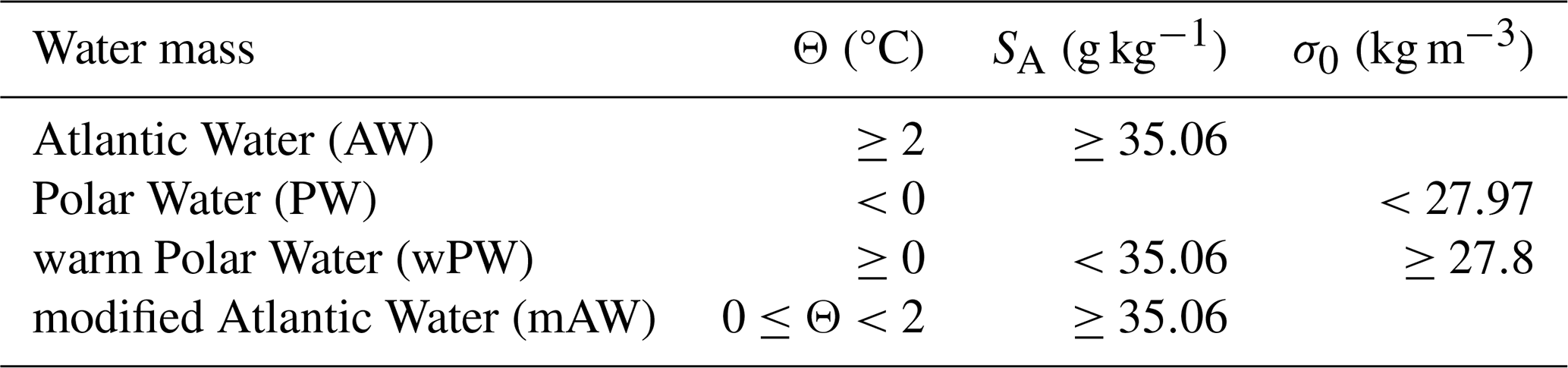
3.1 Water masses
The water masses used in this study are listed in Table 3 and follow Sundfjord et al. (2020). These definitions are based on previous water mass definitions in the literature such as Lind et al. (2018), Loeng (1991) and Rudels et al. (2005). However, we have made a modification to the definition of warm Polar Water (wPW) by including only waters with potential density anomaly σ0≥27.8 kg m−3. By excluding wPW with σ0<27.8 kg m−3, we only consider the wPW, which is a mixture between AW and PW, excluding surface waters influenced to a greater extent by seasonal processes such as atmospheric heating and ice melting. The reason for this is that we miss the surface front (upper 50 m) in all ship transect, and capture it in only a few of the glider transects. The upper 50 m and the water column below are two different domains that are influenced by different physical processes. Here we mainly consider the lower layer.
Table 3Water mass definitions following Sundfjord et al. (2020), using Conservative Temperature, Θ; Absolute Salinity, SA; and potential density anomaly, σ0. Note that our definition of the warm Polar Water includes only waters with σ0≥27.8 in order to exclude surface waters from the wPW.
3.2 Hydrographic sections and geostrophic flow
In order to remove fine-scale variability and obtain fields representative of the background hydrography and geostrophic currents, we produce objectively mapped sections. Along the ship transects, we define a 1 km by 1 m (horizontal by vertical) resolution grid. We objectively interpolate the hydrography data from the ship's CTD system and precision temperature and conductivity sensors of the MSS, and the u and v components of the ocean currents measured by the SADCP, onto the grid using a two-dimensional Gaussian covariance function: , with δ being the Dirac function, e=0.05 being the relative error, and Lx=30 km and Lz=30 m being the correlation scales. Correlation length scales are estimated based on a semi-variogram analysis, similar to that described in Appendix B in Kolås et al. (2020).
Gliders are affected by strong currents that hinder them from collecting data along a straight transect. For the glider data, we first define a transect line by using the best linear fit to the glider surfacing locations. Next, we objectively map the glider Θ and SA at each depth level (1 m vertical resolution) and the glider DAC horizontally onto the new transect at 1 km horizontal resolution, using cov(x,y), Lx=30 and Ly=30 km. Finally, we objectively map Θ and SA along the transect using cov(x,z), Lx=30 km and Lz=30 m (horizontal by vertical) correlation length scales.
The above description produces individual realizations of sections across the front. We also generate a composite section using the profiles from all ship and glider transects to display the average hydrography and geostrophic currents across the PF. The composite section is defined as a 1 km by 1 m (horizontal by vertical) resolution grid along the ship transects across the front (Fig. 2). Next, all hydrography data from the ship's CTD system and the CT sensors of the MSS and gliders were objectively mapped horizontally at each depth level onto the composite grid using a 30 km by 30 km correlation length scale. Similarly, depth-averaged currents from the SADCP and gliders were horizontally mapped onto the composite grid. Hydrography data from gliders and DAC from gliders and SADCP were bin-averaged in 3 km by 3 km horizontal bins before horizontally mapping. A final objective mapping of the hydrography data was performed along the composite grid using Lx=30 km and Lz=30 m.
Because an objectively mapped field is not natural data, errors in Θ and SA can propagate into density calculations and result in spurious unstable layers. To avoid this, we calculated density and, if necessary, rearranged the values to ensure gravitationally stable profiles. To ensure physical consistency, SA was then reproduced from these sorted density fields and Θ. Note, however, that the difference between the originally mapped SA fields and the reproduced fields is minor.
Geostrophic velocity fields relative to the sea surface were calculated using the dynamic height as the geostrophic stream function using the Gibbs-SeaWater library (McDougall and Barker, 2011). We used the objectively mapped Θ and SA sections from the individual transects, as well as the composite sections, to produce relative geostrophic velocity. Finally, we obtain the absolute geostrophic velocity, ug, by removing the depth-averaged relative geostrophic velocity and adding the observed depth-averaged currents from the SADCP or glider in that section.
3.3 Turbulence measurements
When processing the shear probe data to estimate dissipation rates, we followed the recommendations and conventions of the ATOMIX working group (Lueck et al., 2024). We validated our routines against the ATOMIX benchmark datasets (Fer et al., 2024) and successfully reproduced the benchmark estimates.
The dissipation rate of turbulent kinetic energy, ε, was estimated from the spectral analysis of high-pass filtered and despiked time series from the shear probes. Shear spectra were estimated using record lengths of 10 s for the glider/MR and 6 s for the MSS measurements. We used fast Fourier transform (FFT) lengths of 2 s that were cosine-windowed and overlapped by 50 %. Record lengths for spectral calculations (hence, dissipation estimates) were overlapped by 50 %; i.e., dissipation estimates from the MR are at 5 s time resolution, and they are at 3 s from the MSS. Shear spectra were converted from frequency, f, domain to wavenumber, k, domain using Taylor's frozen turbulence hypothesis and the instrument speed through the water, U, as . Here, U is the flow past sensor estimate for the glider and the smooth fall rate for the MSS. The shear spectrum signal coherent with the accelerometer spectrum signal was removed using the Goodman method (Goodman et al., 2006).
Because all dissipation estimates were less than 10−5 W kg−1, the rate of dissipation was estimated by spectral integration. For the glider, the measured shear components are and , where x is pointing along the axis of the instrument. For the MSS profiler, or is measured. Assuming isotropic turbulence, ε was calculated for the probe by integrating the cleaned wavenumber spectrum, Ψ(k):
where ν is the temperature-dependent kinematic viscosity, the overbar denotes averaging in time and an arbitrary shear component is exemplified (e.g., Fer et al., 2014). The lower (k1) integration limit is determined by the wavenumber corresponding to the FFT length, and the upper (ku<∞) integration limit is determined from a minimum in a low-order polynomial fit to the wavenumber spectrum in log–log space. Electronic noise typically takes over after the upper limit, and, to account for the variance in the unresolved part of the spectrum, the model spectrum of Lueck (2022b) was used. This is similar to the empirical Nasmyth spectrum (Nasmyth, 1970), but it is a better-constrained approximation based on more than 14 000 shear spectra. Final dissipation estimates were obtained after quality screening following the ATOMIX recommendations and by averaging the good values from both probes or using the only good estimate. When the fraction of data removed by the despiking algorithm was greater than 5 %, when the figure of merit (a measure of misfit to the model spectrum) relative to the Lueck spectrum was greater than 1.15 or when the difference between dissipation estimates from two probes exceeded the expected statistical uncertainty at 95 % confidence level (Lueck, 2022a), the estimate was flagged as bad. In addition, MSS dissipation measurements obtained from the ship were flagged in the upper 10 m because of the disturbance from the ship’s draft and the profiler’s adjustment to free fall. Noise level of the dissipation rate measured by the MSS and the MR was about and W kg−1, respectively.
3.4 Eddy kinetic energy
Surface geostrophic velocity anomalies from sea-level anomalies obtained from satellite altimeter products (see Sect. 2.6) are used to calculate the surface eddy kinetic energy (EKE):
where uga and vga are the two components of the geostrophic velocity anomalies. For the region over the sill, enclosed by the yellow square in Fig. 1b, we produce a spatially averaged EKE time series covering the duration of our data collection (September 2019 to March 2021). For comparison, an EKE climatology is computed by averaging the monthly EKE over decades in the same region. Finally, we also compute the temporal average EKE at each grid point, averaged over the duration of our data collection. In all EKE estimates, SLA measurements where the SIC was above 15 % have been discarded; hence the average EKE presented here is likely not representative of the region in periods when the region is mainly covered by ice. EKE is known to be stronger when the SIC is low compared to times when the SIC is high (von Appen et al., 2022).
We present data from two scientific cruises conducted in the Barents Sea during October 2020 and February 2021 (referred to as the fall cruise and the winter cruise). The data are supplemented by data from four glider missions across the Barents Sea PF between the Spitsbergen Bank and the Great Bank in the time period 2019–2021.
4.1 Sea surface and atmospheric conditions during the cruises
During the fall cruise, the northwestern Barents Sea was completely free of sea ice, and the sea surface temperature (SST) exceeded 0 °C (Fig. 1b). Only near the eastern coast of Svalbard and in the northernmost region, in the vicinity of the sea ice edge, did the SST decrease below 0 °C. This is in stark contrast to the winter conditions where most of the northwestern Barents Sea was covered by sea ice, and the 0 °C surface isotherm closely followed the 200 m isobath (Fig. 1c). The surface signature of the AW inflow is confined to the waters where the seafloor depth exceeds 200 m, both during fall and winter.
Our study region is centered at the topographic sill between the Hopen Trench and the Olga Basin, and it covers the PF region where AW from the south flows beneath PW to the north (yellow square, Fig. 1b and c). Changing winds shift surface waters, affecting the surface temperature and sea ice concentration (Fig. 1d and e). Most pronounced are the wind events at the beginning of February 2020 and in late February 2021, when southerly winds changed the average sea ice concentration over the sill from nearly 100 % to less than 15 % over the course of a week. In addition, southerly winds lasting for nearly 1.5 months in December 2020 and January 2021 kept the region above the sill nearly ice-free until February 2021. During the previous winter, however, the sea ice concentration in the region above the sill rose gradually from early December 2019 to mid-February 2020.
While the surface conditions in the study region are highly influenced by the local surface winds, the properties and variability of the deeper layers are more resilient to the rapidly shifting winds and may be affected by other forcing mechanisms. Next, we look at the vertical and latitudinal structure of the PF across the sill, focusing on the oceanic drivers of variability.
4.2 Polar Front structure and seasonal variability
A total of 16 ship and glider transects were conducted during late summer, fall and winter 2019–2021. Of these, 11 were conducted during October and November and have been combined into a fall composite, while 4 were collected during December and February and have been combined into a winter composite (Fig. 3a and b, respectively). Note that 1 transect conducted during August was not included in the seasonal composites. The method for combining data from individual transects into a composite section is described in Sect. 3.2. During fall, a 50 m thick surface layer with warm (> 1.5 °C) and fresh (< 34.6 g kg−1) water is present, and the PF is located below the surface layer. The center of the PF is highlighted by the 0 °C isotherm, a threshold practically identical to the 0.1 °C determined by Kolås (2024, Chap. 3.2.7). The PF, roughly 30 km wide during fall (−1 °C °C at about 100 m depth), separates a subsurface AW core on the southern side of the sill from PW on the northern side (Fig. 3a). The subducted AW core is separated from the surface layer by a colder, 25 m thick, interleaving layer at about 60 m depth. The overall PF structure during fall is similar to that from ship and glider transects collected during October and early November 2020 (Figs. 4 and 5). Note, however, that the glider transects in general exhibit more variability in the PF structure than the ship transects. The short-term variability is described in Sect. 4.3.

Figure 3Composite section combining hydrography and current data from the individual ship and glider transects. (a) Fall composite combining data collected during October and November (11 transects), (b) winter composite combining data collected during December and February (4 transects), and (c) average composite combining all the individual transects (16 transects when including the August transect). From left to right, the different columns show Conservative Temperature, Θ; Absolute Salinity, SA; and absolute geostrophic velocity, ug. Positive values of ug are eastward. The white line (left) is the 0 °C isotherm, indicating the center of the Polar Front when below 50 m depth. Black contours (right) show isopycnals. The horizontal axis is the northward distance relative to the crest of the sill separating the Hopen Trench in the south from the Olga Basin in the north.
From fall to winter, waters on both sides of the front cool, and the warm and fresh surface layer transitions into PW, becoming colder and more saline (Fig. 3b). During winter, PW reaches about 60 km farther south than during fall, extending to about −55 km relative to the saddle point of the sill. On the other hand, mAW and wPW below 125 m depth extend 5–10 km farther north during winter than during fall, reaching about 25–30 km north of the sill. By combining data from all the individual transects we produce an average composite section (Fig. 3c). The composite section shows that, on average, the front is located between 10 km south and 25 km north of the sill, starting at 50 m depth on the southern side and extending to the seabed on the northern side. Note, however, that the bulk of our data is collected during fall, and the composite is biased towards “fall conditions”. The across-front gradients of Θ and SA calculated from the average composite section, between ±20 km of the 0 °C isotherm at 100 m depth, are −0.06 °C km−1 and −0.008 g kg−1 km−1, respectively (Fig. 3 and Table 4). The 100 m depth was chosen, as it is typically where the subsurface warm core is located south of the front. Averaging in the composite section smooths the front, and the mean values of the gradients calculated from the individual transects are larger: °C km−1 and g kg−1 km−1 (± 1 standard deviation).
Table 4Transport estimates for the frontal jet and gradients across the front for the composite sections and the individual transects shown in Figs. 3, 4 and 5. Dates correspond to the dates of the individual transects as shown in Figs. 4 and 5. The fall composite combines data collected during October and November (11 transects), the winter composite combines data collected during December and February (4 transects), and the average composite combines all the individual transects (16 transects). Volume transport estimates (positive eastward) are given for the frontal jet where it is captured. Gradients are calculated between ± 20 km of the 0 °C isotherm at 100 m depth. In the few cases where the transect does not extend ± 20 km of the 0 °C isotherm, the gradient is calculated from the edge of the transect. Mean and standard deviation (± SD) values are calculated from the individual transects.
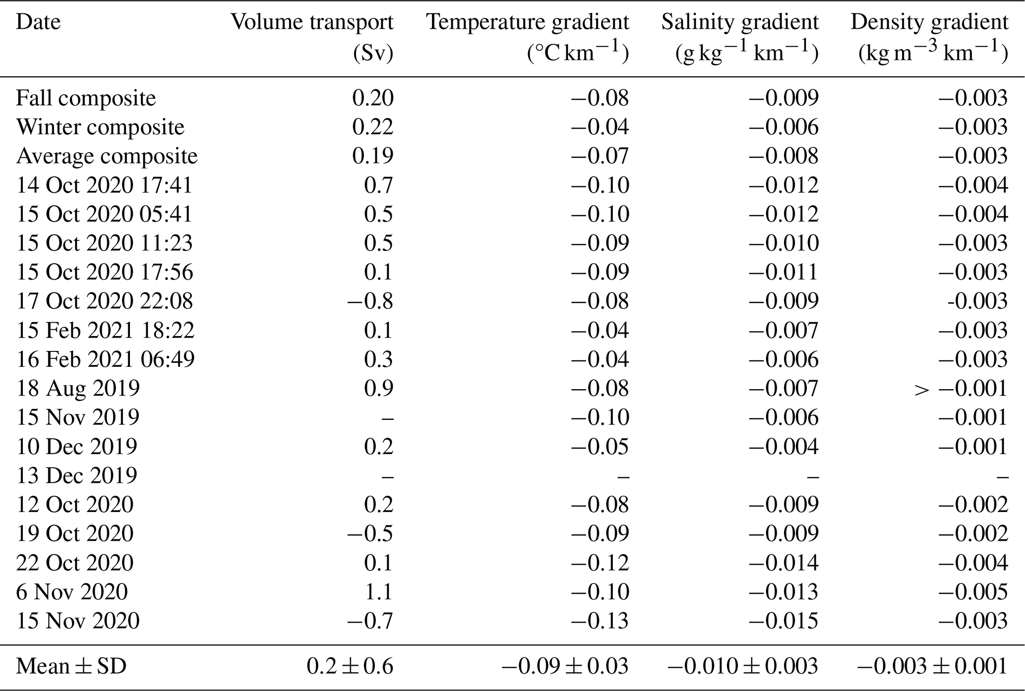
Throughout most transects, the horizontal temperature and salinity gradients below the surface layer result in a baroclinic front with density lines sloping downward as they cross the front. This is captured in the composite sections (Fig. 3). On the warm side of the front, during fall, water with σ0=27.8 kg m−3 resides about 70 m higher up in the water column than on the cold side of the front (Fig. 3a). Subsequently, a bottom-intensified eastward geostrophic current is generated with an estimated volume transport of 0.2 Sv. During winter, the frontal region extends about 50 km farther south. The 27.8 kg m−3 isopycnal outcrops at −55 km, suggesting water with equal density resides 150 m higher up in the water column south of the front compared to north of the front (Fig. 3b). Nevertheless, the slope of the isopycnal across the front and the eastward volume transport during winter are similar to those during fall (Table 4). Furthermore, the position of the frontal current is also similar during fall and winter, with the core of the current located about 10 km north of the sill. The average transport by the frontal current, calculated as the average from the individual transects, is 0.2±0.6 Sv, where ± 0.6 denotes the standard deviation over the individual transects. The variability is relatively large, ranging between 1.1 and −0.8 Sv. Negative volume transports are due to reversals of the geostrophic current (Fig. 4c and c), which are discussed in Sect. 4.3. If we exclude the reversal events (three transects), the mean eastward volume transport becomes 0.4±0.4 Sv.
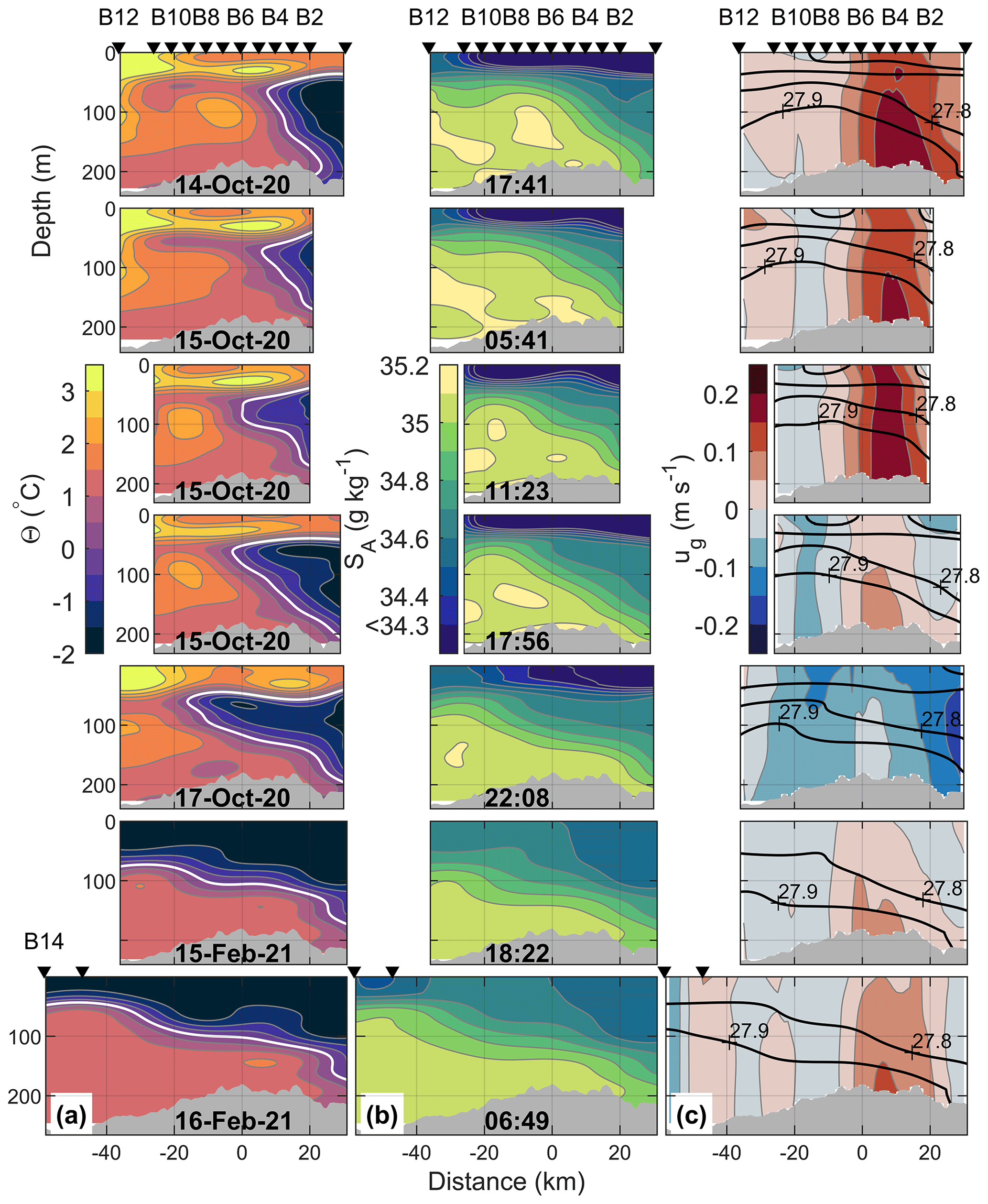
Figure 4Repeated hydrographic measurements from the ship across the Polar Front and the sill separating the Hopen Trench and the Olga Basin (Figs. 1 and 2). (a) Conservative Temperature, Θ; (b) Absolute Salinity, SA; and (c) absolute geostrophic velocity, ug (positive eastward). The white line in panel (a) is the 0 °C isotherm, indicating the center of the Polar Front when below 50 m depth. Black contours in panel (c) show isopycnals at 27, 27.4, 27.8 and 27.9 kg m−3. The date and time (UTC) of the station at the crest of the sill are given in panels (a) and (b), respectively. The horizontal axis is the northward distance relative to the crest of the sill (0 km), and black triangles at the top indicate station locations with names. Bottom topography (gray) is from the ship's echo sounder. The vertical axis is scaled so that the height of 100 m depth is equal in all panels.

4.3 Short-term variability at the Polar Front
Between 15 and 17 October 2020 the eastward geostrophic current on the sill weakened and reversed, flowing westward (Figs. 4 and 5). Simultaneously, the maximum southward extension of the PF increased by more than 25 km. We propose that this change was caused by an anticyclonic eddy in the Olga Basin north of the sill.
Satellite observations of the SLA suggest an anticyclonic eddy developed after 12 October, north of the sill (Fig. 6a). This eddy moved south while it picked up in strength, reaching a maximum on 19 October, before leaving the site after a few days. The geostrophic velocity anomalies calculated from the SLA agree well with the glider DAC (Fig. 6a). Note, however, that the DAC from the glider also measures the frontal current; hence the glider DAC and the surface geostrophic velocity anomalies calculated from the SLA are not expected to be equal.
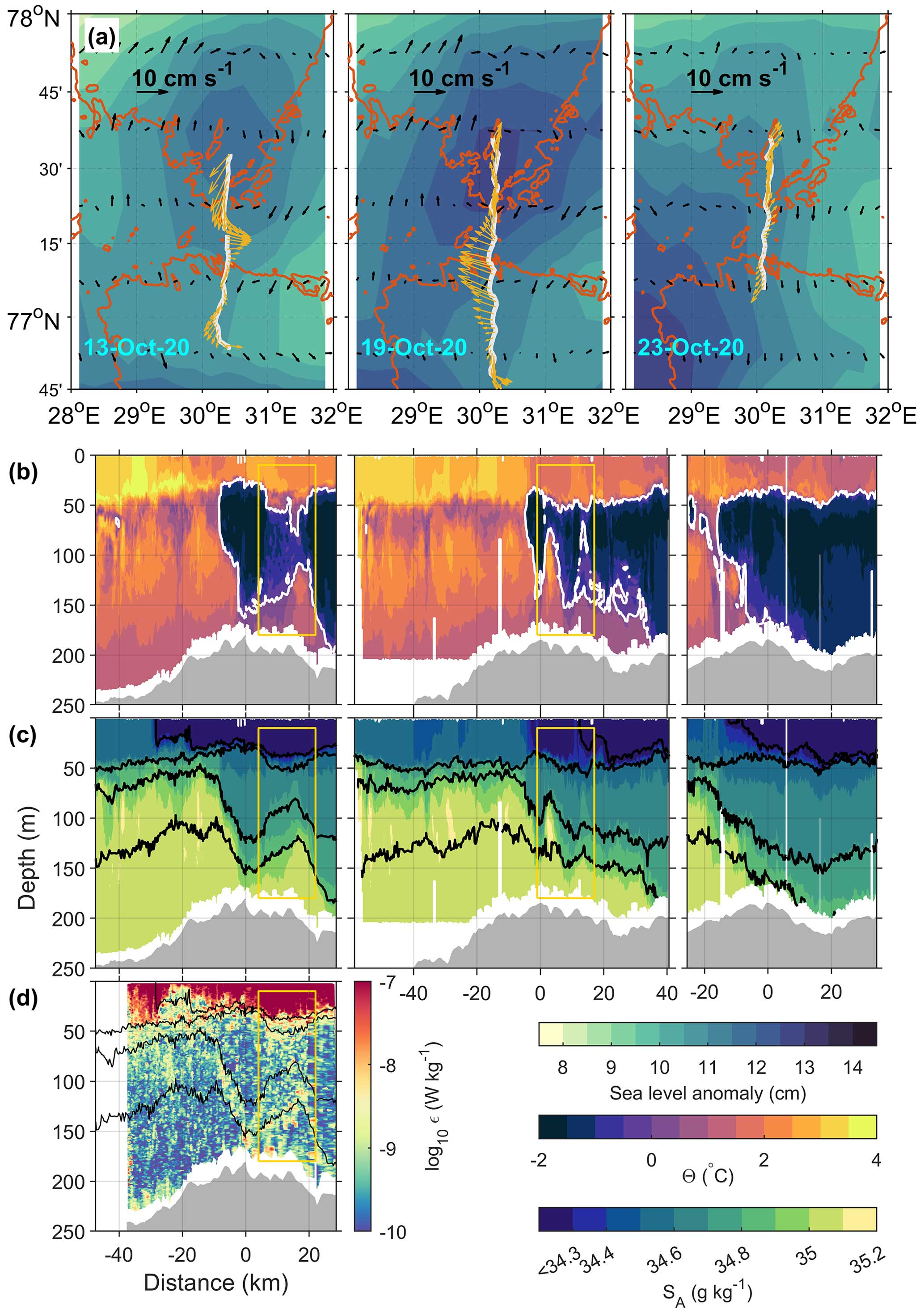
Figure 6Three crossings over the sill with the Slocum glider Odin in October 2020. (a) Sea-level anomalies and the surface geostrophic velocity anomalies (black quivers) on the date specified in the lower-left corner. The white line shows the glider track, and the yellow quivers show the glider DAC. (b) Conservative Temperature, Θ, and (c) Absolute Salinity, SA, along the three glider crossings shown in panel (a). (d) Dissipation rate of turbulent kinetic energy, ε, along the first glider transect shown in panel (a) (turbulence instrument stopped recording after the first transect). The white line in panel (b) is the 0 °C isotherm, and the black lines in panels (c) and (d) are the 27.2, 27.6, 27.8 and 27.9 kg m−3 isopycnals. The glider transects shown in panels (b) and (c) are the same as the October transects in Fig. 5 but without objective mapping or along-path smoothing. The yellow boxes enclose the position of, and region most affected by, the eddy. Bottom topography (gray) is from IBCAO-v4.
The surface signature of the eddy (anomalously high positive sea level) is supplemented by the subsurface data from the glider (Fig. 6b and c). The eddy is a cold-core eddy, and as it moves south towards the PF, warmer water from above is pulled down, and warmer and saltier water from below is lifted up (yellow boxes, Fig. 6b–c). Subsequently, as the eddy moves across the front, the steepness of the isopycnal slope is reduced, suggesting the eddy consumed some of the available potential energy in the baroclinic front (middle panel, Fig. 6c).
The anticyclonic eddy traversing the PF during mid-October 2020 is not a unique occurrence. Between 6 and 15 November 2020, a warm-core anticyclonic eddy moved northward up the Hopen Trench (Fig. 5, lower two panels). This eddy, also supported by satellite SLA observations (not shown here), transports warmer AW from further south towards the front, resulting in increased temperatures on both sides of the front and a relaxation of the isopycnal slope.
While accounting for much of the variability observed across the PF, eddies do not explain all of it. The glider transects conducted between 10 and 13 December 2019 suggest the PF has shifted 20–40 km northward in the span of 3 d (Fig. 5). This is likely not the case. The transect on 13 December is the easternmost transect across the sill, about 25 km east of 30° E (see glider sections shown in Fig. 2), and does not extend as far north relative to the highest point on the sill as most of the other transects do. Hence it is likely that the transect failed to capture the front as a result of spatial variability but not temporal variability.
Another source for temporal variability at the PF is tidal currents. Stations occupied for 12 h with half-hourly repeated MSS casts conducted during both cruises showed that tidal currents dominated short-term current variability at the PF during the fall and winter cruises (Fig. 7a, d). The observed depth-averaged currents reach a maximum northward velocity of ∼ 15 cm s−1 during both fall and winter. While the following southward flow is similarly strong during fall, it only reaches about 5 cm s−1 during winter. Note that on 18 October, the eddy displayed in Fig. 6a is close to the repeated station. The azimuthal velocity of the rim of the eddy, with a west-southwestward component, may be responsible for the systematic deviation of the DAC from the Arc2km tidal currents (Fig. 7a). During fall, maximum northward velocities are accompanied by substantial warming in the middle of the water column (Fig. 7b). This may be interpreted as a northward displacement of the front, allowing warmer AW to reach the measurement station throughout the water column. During winter, this is not visible, possibly due to the nearly horizontal nature of the front (lower two panels of Fig. 4). The suspected lateral displacement of the front during the fall cruise does not coincide with any significant changes in the layer-integrated dissipation rates (Fig. 7c). However, during winter, peak tidal currents are associated with an increased dissipation rate in the deeper part of the water column (Fig. 7f). The vertically integrated dissipation rate, , where ρ=1025 kg m−3 and z1 and z2 are the bounds of the layers over which integration is made, indicates the total dissipation rate per unit surface area and can be related to work done, for example, by tidal currents. In winter, Dε in the deeper part of the water column accounted for a substantial fraction of the dissipation in the water column below the surface layer.
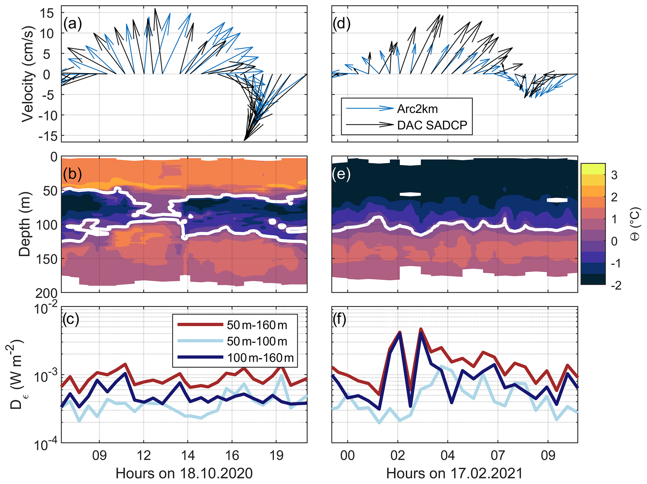
Figure 7Repeat stations every 12 h at B5 in fall (a–c) and B7 in winter (d–f). Total depth is 192 and 185 m for B5 and B7, respectively, and the station location is indicated in Fig. 2. (a, d) Time series of depth-averaged currents (DACs) together with tidal currents from the Arc2km model (Howard and Padman, 2021), (b, e) temperature with the white line marking the 0 °C isotherm and (c, f) dissipation rate vertically integrated over different layers Dε indicated in the legend. The maximum layer depth is set to 160 m to be consistent with the few profiles that do not extend deeper.
The tidal v component is likely to have a greater impact on the frontal structure than the u component, as the front is aligned west–east. However, the relatively weak north–south tidal oscillation is unlikely to shift the water any more than about 1 km within a tidal period, with minimal effect on the frontal structure and geostrophic balance. Nevertheless, tidal-induced velocity shear may generate mixing, which again may erode the frontal structure.
4.4 Mixing across the Polar Front
Microstructure measurement transects were conducted from the ship across the front in the fall and winter cruises and also by the glider in October 2020. Most of the observed mixing occurs within the surface boundary layer, where estimates of dissipation rate of turbulent kinetic energy (ε) exceed 10−6 W kg−1 (Figs. 6d and 8).

Figure 8Dissipation rate of turbulent kinetic energy, ε, estimated from the MSS profiler during the fall (upper five panels) and winter (lower two panels) cruises. Black lines show isopycnals at 27.2, 27.6, 27.8 and 27.9 kg m−3. Tidal currents during the transects are shown in the right panels. Colors indicate the individual transects, with S or N indicating whether the section started from the south or north end, respectively.
In October, the surface mixed layer (upper 60 m or so) is separated from the deeper layer by a strongly stratified pycnocline, where mixing quickly abates. In February, however, the stratification in the pycnocline is weaker, and surface mixing occasionally extends down to 100 m depth. Below the surface mixed layer, most of the mixing occurs in the bottom boundary layer, where ε reaches 10−7 W kg−1 (Figs. 6d and 8). Mixing in the bottom boundary layer is strongest during the first October ship transects when the geostrophic current is at its strongest (Fig. 8; upper two panels). At the front, where Θ and SA gradients are strong, we observe elevated dissipation rates occasionally reaching 10−7 W kg−1. This is particularly visible during the glider transect, where we have microstructure profiles at every 500 m interval across the front. Here, elevated dissipation rates follow the 0 °C isotherm closely, marking the transition and mixing between mAW and PW (Fig. 6b and d). In the interior, away from the front, estimates of ε are often at the noise level of the instrument, indicating little or no mixing.
The role of the PF as a mixing zone is highlighted by the observed water mass transformation across the front, in the Θ–SA space (Fig. 9). Profiles from the front region are shown together with those from Sect. D in the south and those from Sect. A and F in the north (see section locations in Fig. 2). About 60 km south of the highest point on the sill, the water column is composed of AW and mAW (Fig. 9, Sect. D). These water masses have mainly been modified through cooling by the atmosphere during their transit from the BSO toward the Hopen Trench. However, as the AW enters the frontal region, AW mixes directly with PW residing north of the PF in the Olga Basin, generating wPW (Figs. 9 and 2). The wPW is transported eastward by the geostrophic current along the front and is found downstream northeast of the sill (Fig. 9, Sect. A).
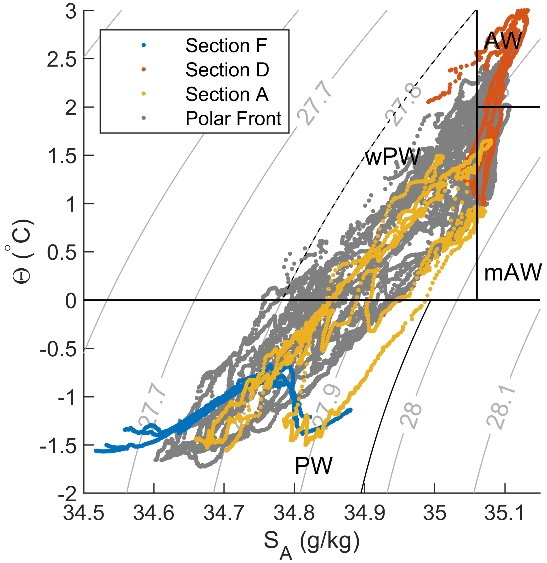
Figure 9Θ–SA diagram showing water masses around and across the Polar Front, below 80 m depth. Blue, yellow and red profiles correspond to the profiles along the indicated sections, marked with the same color in Fig. 2. Polar Front profiles (gray) are profiles collected between stations B2 and B11. All profiles are from the fall cruise.
5.1 Barents Sea Polar Front structure and seasonal change
Previous studies on the western Barents Sea PF have been conducted along the southern and southeastern slopes of the Spitsbergen Bank (Loeng, 1991; Gawarkiewicz and Plueddemann, 1995; Parsons et al., 1996; Harris et al., 1998; Fer and Drinkwater, 2014) and along the southwestern slope of the Great Bank (Våge et al., 2014). These studies describe the PF in the western Barents Sea, below the surface layer, as a barotropic front with horizontal density lines. The PF we observe across the sill between the Spitsbergen Bank and the Great Bank differs from these observations. We observe a baroclinic front where isopycnals tilt downwards with distance from south to north across the front (Figs. 3, 4 and 5). Subsequently, a bottom-intensified geostrophic flow develops. A likely reason for this difference in the frontal structure is the difference in the bathymetry. While the seabed on the Spitsbergen Bank and the Great Bank rises to above 100 m depth, the highest point on the sill is 180 m deep. Along the slopes on the banks the seabed serves as a boundary, blocking the AW. Across the sill, AW can flow without the same topographic boundary, and consequently a geostrophic adjustment balances the inflowing AW and the overlaying PW.
The upper 50–80 m of the water column across the topographic sill is largely affected by seasonal variability (Fig. 3a and b). Through August to early November, relatively warm (> 2 °C) and fresh (<34.3 g kg−1) water resides in the surface layer, suggesting atmospheric heating of seasonal meltwater (Figs. 4 and 5). By February, nearly all of the surface layer is occupied by PW (< 0 °C), and the salinity has increased (> 34.6 g kg−1), reducing the strong stratification in the pycnocline observed during fall and extending the PF more or less to the surface. The increased surface salinity during winter is likely due to brine rejection from sea ice formation. This seasonality is similar to the seasonality previously described along the southern slope of the Spitsbergen Bank (Harris et al., 1998).
In contrast to the seasonal change observed in the upper 100 m, the position of the front below 100 m is relatively stable from fall to winter (Fig. 4). However, the position of the incropping of the 0 °C isotherm on the north side of the sill varies by about 10 km, suggesting that the AW overflow across the sill below 100 m depth exhibits some seasonal variability. The temperature and salinity in the bottom 50 m above the sill remain above 1 °C and 35 g kg−1 between October and February, suggesting little seasonal change. Nevertheless, there is more mAW and wPW in the bottom 50 m, north of the sill, during winter compared to fall. This suggests a larger influence of warm water in the bottom layer during winter than during fall, although temperatures south of the front in general are lower during winter compared to fall.
The difference in seasonality between the upper and lower layer (above and below 100 m depth) has consequences for the PF structure. During fall, the 0 °C isotherm, particularly between 50–100 m depth, is typically inclined from the horizontal and is occasionally vertical, while it is nearly horizontal during winter. Oziel et al. (2016) describe the PF position as the isotherm corresponding to the modal temperature in the region with the highest horizontal temperature gradients in the 50–100 m layer. While this may be representative of the PF location during fall, it is less suitable during winter as the temperature front becomes nearly horizontal, spanning almost 100 km. Nevertheless, the density gradient across the front at 100 m depth remains similar from fall to winter and is on average kg m−3 km−1 (Fig. 3 and Table 4). This is about 1/10 of the density gradient across the surface density front observed by Parsons et al. (1996). However, the surface and subsurface fronts are two different domains and are not directly comparable. Most frontal studies in the Barents Sea have studied the subsurface temperature and salinity gradients individually, as they tend to be density-compensating (Oziel et al., 2016; Barton et al., 2018). However, estimated from Fig. 7 in Barton et al. (2018), the 1985–2016 average density gradient across the Ludlow Saddle in the Barents Sea, at 100 m depth, is approximately −0.003 kg m−3 km−1, similar to our findings.
5.2 Short-term variability
The middle layer of the water column above the sill (roughly between 50–130 m depth) is highly dynamic, particularly during fall and early winter when the temperature and salinity fronts are more vertical than during winter (Figs. 4 and 5). In October we observe the position of the front, marked by the 0 °C isotherm, shifting nearly 25 km over the span of 3 to 4 d (Fig. 4). The two main drivers of this short-term variability (below 50 m depth) are tidal currents and mesoscale eddies.
The tidal currents observed above the sill have a peak-to-peak variability of about 30 cm s−1 during fall and 20 cm s−1 during February (Fig. 7a and d). During fall, when the temperature front is nearly vertical, tidal currents shift warm and cold water back and forth. The north–south displacement of water masses is roughly 2 km when assuming an average tidal current of 10 cm s−1 during 6 h. Nevertheless, the tidal-induced mixing is mainly confined to the bottom 30 m with little contribution to mixing at mid-depth, both during fall and winter (Figs. 7 and 8). For comparison, Fer and Drinkwater (2014) observed tidal currents with a peak-to-peak variability of about 50 cm s−1 on the southeastern slope of the Spitsbergen Bank during May 2008. As a result, estimates of ε exceeded 10−6 W kg−1 near the seabed, and the entire water column was well-mixed where the bank was shallower than about 75 m. We expect the contribution from mixing due to tidal currents to have large spatial variability along the PF, depending much on the local topography. Note that we observe mixing rates in the surface layer (upper 50 m) that are much higher than mixing rates in the lower layer throughout all of our observations, mainly exceeding 10−7 W kg−1 (Figs. 6d and 8). This is comparable to previous mixing rates observed on the sill between the Hopen Trench and the Olga Basin. Sundfjord et al. (2007) found an average dissipation rate of W kg−1 across the pycnocline in May 2005 and stated that the average dissipation rates within the pycnocline were at least 5 times larger than that below the pycnocline.
In October and November 2020, we observed two eddies modifying the structure of the PF across the sill between the Hopen Trench and the Olga Basin (Sect. 4.3 and Figs. 5 and 6). Porter et al. (2020) similarly observed a surface eddy further south along the Hopen Trench during July 2017. This eddy originated from the Arctic region in the Barents Sea and traveled south along the Spitsbergen Bank (Porter et al., 2020). Eddy kinetic energy calculated from satellite-derived surface geostrophic velocity anomalies suggests the slope between the Spitsbergen Bank and the Hopen Trench is a region where eddies commonly occur (Fig. 10a). In addition, EKE averaged over the sill between the Hopen Trench and the Olga Basin suggests several eddies were present between August 2019 and April 2021 (Fig. 10b). Note, however, that the eddy observed in mid-October 2020 (shown in Fig. 6) does not appear in the time series of the average EKE over the sill, likely due to a mismatch between the averaging box and the position of the eddy. Hence, the time series is likely an underestimate of the eddy energetics during our study period. In addition, only the largest eddies will have a surface SLA signal detectable by satellites, as the SLA resolution is 0.25°. Accordingly, as the PF across the sill is baroclinic, eddies too small to be detectable by satellite altimetry may shed from baroclinic instabilities, feeding off the available potential energy across the front. Atadzhanova et al. (2018) observed about 3000 eddy structures in the Barents Sea during June–October 2007 and 2011, of which 25 % occurred in the region around the PF. These eddies were determined from radar images and had a mean diameter of about 4 km. Most eddies at that scale will likely not be detectable by sea-level height measurements. In addition, Porter et al. (2020) state that the eddy they detected in the southern Hopen Trench was thermally capped; that is, the surface of the eddy had lost its cold-core characteristics and was indistinguishable from surrounding waters using satellite imagery. This suggests that even the number of eddies observed by Atadzhanova et al. (2018) could be an underestimation of the eddies present in the Barents Sea.

Figure 10Eddy kinetic energy estimated from satellite-derived surface geostrophic velocity anomalies, based on sea-level anomalies. (a) Temporal average between 1 August 2019 and 1 April 2021, covering the data collection period. The black line is the 200 m isobath, and the white line encloses the region used for the spatial average in panel (b). (b) The blue line shows the spatially averaged daily EKE over the region enclosed by the white line in panel (a) for the duration of our data collection period. Gray shading shows the standard deviation of the averaged EKE. Red and yellow lines show the monthly decadal mean for the same region.
A comparison of the 10-year monthly averaged EKE suggests that eddies in the northwestern Barents Sea are most energetic during winter, by a factor of 2 relative to summer (Fig. 10b). This is in contrast to the observations by Atadzhanova et al. (2018), who find the peak eddy activity to be in July. Note, however, that SLA measurements where the SIC was above 15 % have been discarded (see Sect. 3.4). This could lead to a potential bias towards higher EKE during winter, as we only include the most energetic regions (ice-free regions) during winter. Our 10-year monthly averaged EKE is likely only representative of the region when most of the region enclosed in Fig. 10a is ice-free.
Comparing the 2000–2009 decade to the 2010–2019 decade suggests that the EKE in general has increased in the region. The reason for this increase in EKE is not clear. The volume transport through the BSO is closely linked to the North Atlantic Oscillation (NAO) and local winds (Heukamp et al., 2023). An increased volume flux into the Barents Sea caused by faster, more energetic currents could potentially lead to an increase in observed EKE in the Barents Sea. However, there is little evidence supporting any significant difference in the volume flux through the BSO between 2000 and 2019 (Heukamp et al., 2023; Årthun et al., 2019). We suggest the increase in EKE may be related to the observed increase in oceanic heat transport into the Barents Sea and the subsequent decrease in sea ice extent, the so-called Atlantification of the Barents Sea (Skagseth et al., 2008; Årthun et al., 2012; Barton et al., 2018; Årthun et al., 2019).
This study provides insights into the dynamics and hydrography of the Barents Sea Polar Front within the region bounded by the Hopen Trench and the Olga Basin in the Barents Sea. The topographic sill separating the Hopen Trench from the Olga Basin is a location where AW meets PW, setting up a front where AW eventually subducts below PW. The data presented herein were collected during two scientific cruises in October 2020 and February 2021 and during four glider missions spanning 2019 to 2021.
During the fall cruise, the western Barents Sea was devoid of sea ice, with sea surface temperatures mainly exceeding 0 °C. In February, however, the northwestern Barents Sea and the sill separating the Hopen Trench and the Olga Basin were covered by sea ice, with the 0 °C isotherm aligning closely with the 200 m isobath. Despite the seasonal changes at the surface and in the surface mixed layer, the influence of the AW inflow near the seabed over the sill remained unperturbed.
This study shows that the PF over the sill is a distinct baroclinic front supporting an eastward geostrophic current above the sill. The average eastward transport of this current is estimated to 0.2±0.6 Sv, where ± 0.6 denotes the standard deviation over 16 repeat transects. The baroclinic front differs markedly from prior observations along the Spitsbergen Bank and Great Bank slopes, where a barotropic front with horizontal density lines was typically noted. The distinction arises from variations in bathymetry, as the absence of a topographic boundary permits a geostrophic adjustment to balance inflowing AW and overlying PW.
The upper layers of the PF (0–100 m) experienced pronounced seasonal fluctuations, influenced by atmospheric heating, sea ice formation, and brine rejection. However, the position of the front beneath 100 m depth exhibited minimal seasonal variability.
Short-term variability stemmed from tidal currents and mesoscale eddies. Tidal currents induced 2–4 km north–south displacement of water masses, especially notable when the subsurface temperature front was approximately vertical. However, the modification of the PF by tidal currents was negligible compared to the effects of mesoscale eddies. Observations collected from ships and gliders, as well as satellite altimetry data, independently indicated the presence of two eddies at the PF in October and November 2020. These eddies influenced the front's structure, shifting the position of the front as much as 25 km in less than 4 d. In addition, the isopycnal slope across the front was markedly reduced after the passage of an eddy, suggesting the eddy reduced the available potential energy of the front during its traversing of the front. Simultaneously, as the eddy approached the front, the satellite-derived SLA showed the eddy's radial velocity increasing, suggesting the available potential energy was converted to EKE.
Microstructure measurements showed intense mixing within the surface boundary layer, particularly in the upper 60 m. During winter, this mixing extended occasionally to 100 m. Below the surface layer, significant mixing was concentrated in the bottom boundary layer and linked to the tidal oscillations across the sill. Nevertheless, we observed substantial water mass transformation across the front, which was likely a result of eddy-driven along-isopycnal mixing.
This study offers a comprehensive description of the Barents Sea Polar Front, shedding light on its interactions with seasonal shifts, tidal currents and mesoscale eddies. The distinctive baroclinic structure observed across the topographic sill underscores the importance of local bathymetry in shaping front dynamics.
All data presented in this study are openly available. Hydrography, current and microstructure data collected during the October 2020 and February 2021 cruises are available from Fer et al. (2023a), Fer et al. (2023d), Fer et al. (2023e) and Fer et al. (2023b). Glider data are available from Kolås et al. (2022), and the microstructure data collected by Odin are available from Fer et al. (2023c). Sea ice concentration is from OSI-SAF (2017), sea surface temperature is from Copernicus (2019), daily and monthly sea-level anomalies are from Copernicus (2023), and bathymetry data are from Jakobsson et al. (2020). The Arctic 2 km Tide Model (Arc2kmTM) can be downloaded from the Arctic Data Center at https://doi.org/10.18739/A2PV6B79W (Howard and Padman, 2021).
IF, TMB and EHK collected the data in addition to conceiving and planning the analysis. EHK, IF and TMB performed the analysis. EHK wrote the paper, with advice and critical feedback from IF and TMB. All authors discussed the results and finalized the paper.
At least one of the (co-)authors is a member of the editorial board of Ocean Science. The peer-review process was guided by an independent editor, and the authors also have no other competing interests to declare.
Publisher’s note: Copernicus Publications remains neutral with regard to jurisdictional claims made in the text, published maps, institutional affiliations, or any other geographical representation in this paper. While Copernicus Publications makes every effort to include appropriate place names, the final responsibility lies with the authors.
This work was supported by the Nansen Legacy Project. We thank the officers, crew and scientists of the R/V G.O. Sars cruise in October 2020 and the R/V Kronprins Haakon cruise in February 2021. We thank the glider team at NorGliders (http://norgliders.gfi.uib.no/, last access: 2 July 2024) for operating and maintaining all the glider missions in challenging conditions in the Barents Sea.
This research has been supported by the Research Council of Norway (grant no. 276730).
This paper was edited by Katsuro Katsumata and reviewed by two anonymous referees.
Årthun, M., Ingvaldsen, R., Smedsrud, L., and Schrum, C.: Dense water formation and circulation in the Barents Sea, Deep-Sea Res. Pt. I, 58, 801–817, https://doi.org/10.1016/j.dsr.2011.06.001, 2011. a
Årthun, M., Eldevik, T., Smedsrud, L. H., Skagseth, Ø., and Ingvaldsen, R. B.: Quantifying the Influence of Atlantic Heat on Barents Sea Ice Variability and Retreat, J. Clim., 25, 4736–4743, https://doi.org/10.1175/JCLI-D-11-00466.1, 2012. a
Årthun, M., Eldevik, T., and Smedsrud, L. H.: The Role of Atlantic Heat Transport in Future Arctic Winter Sea Ice Loss, J. Clim., 32, 3327–3341, https://doi.org/10.1175/JCLI-D-18-0750.1, 2019. a, b
Atadzhanova, O., Zimin, A., Svergun, E., and Konik, A.: Submesoscale Eddy Structures and Frontal Dynamics in the Barents Sea, Phys. Oceanogr., 25, 220–228, https://doi.org/10.22449/1573-160X-2018-3-220-228, 2018. a, b, c, d, e
Barton, B. I., Lenn, Y.-D., and Lique, C.: Observed Atlantification of the Barents Sea Causes the Polar Front to Limit the Expansion of Winter Sea Ice, J. Phys. Oceanogr., 48, 1849–1866, https://doi.org/10.1175/JPO-D-18-0003.1, 2018. a, b, c
Carrere, L., Faugère, Y., and Ablain, M.: Major improvement of altimetry sea level estimations using pressure-derived corrections based on ERA-Interim atmospheric reanalysis, Ocean Sci., 12, 825–842, https://doi.org/10.5194/os-12-825-2016, 2016. a
Copernicus: Arctic Ocean – Sea and Ice Surface Temperature, Copernicus Marine Service [data set], https://doi.org/10.48670/moi-00130, 2019. a, b, c
Copernicus: Global Ocean Gridded L 4 Sea Surface Heights And Derived Variables Reprocessed 1993 Ongoing, Copernicus Marine Service [data set], https://doi.org/10.48670/moi-00148, 2023. a, b
Crews, L., Sundfjord, A., Albretsen, J., and Hattermann, T.: Mesoscale Eddy Activity and Transport in the Atlantic Water Inflow Region North of Svalbard, J. Geophys. Res.-Ocean., 123, 201–215, https://doi.org/10.1002/2017JC013198, 2018. a
Fer, I. and Drinkwater, K.: Mixing in the Barents Sea Polar Front near Hopen in spring, J. Mar. Syst., 130, 206–218, https://doi.org/10.1016/j.jmarsys.2012.01.005, 2014. a, b, c, d, e, f, g, h
Fer, I., Peterson, A. K., and Ullgren, J. E.: Microstructure Measurements from an Underwater Glider in the Turbulent Faroe Bank Channel Overflow, J. Atmos. Ocean. Technol., 31, 1128–1150, https://doi.org/10.1175/JTECH-D-13-00221.1, 2014. a, b
Fer, I., Skogseth, R., Astad, S. S., Baumann, T., Elliott, F., Falck, E., Gawinski, C., and Kolås, E. H.: SS-MSC2 Process cruise/mooring service 2020: Cruise Report, The Nansen Legacy Report Series, https://doi.org/10.7557/nlrs.5798, 2021. a
Fer, I., Baumann, T. M., Elliot, F., and Kolås, E. H.: Ocean microstructure measurements using an MSS profiler during the Nansen Legacy cruise, GOS2020113, Norwegian Marine Datacentre [data set], https://doi.org/10.21335/NMDC-239170563, 2023a. a, b, c, d, e
Fer, I., Baumann, T. M., Koenig, Z., Randelhoff, A., Rieke, O., Hana, I., and Årvik, A.: Ocean hydrography and current profiles from the Nansen Legacy Process Cruise to the Barents Sea, KB2022625, Norwegian Marine Datacentre [data set], https://doi.org/10.21335/NMDC-943526062, 2023b. a, b, c, d
Fer, I., Kolås, E. H., and Elliot, F.: Dissipation measurements from a Slocum glider at the Barents Sea Polar Front, Norwegian Marine Datacentre [data set], https://doi.org/10.21335/NMDC-1033548414, 2023c. a, b, c, d
Fer, I., Nilsen, F., Baumann, T. M., Kalhagen, K., Koenig, Z., and Kolås, E. H.: Ocean hydrography and current profiles from the Nansen Legacy Winter Process Cruise to the northern Barents Sea, KH2021702, Norwegian Marine Datacentre [data set], https://doi.org/10.21335/NMDC-1544015310, 2023d. a, b, c, d, e
Fer, I., Skogseth, R., Astad, S., Baumann, T., Elliot, F., Falck, E., Gawinski, C., Kalhagen, K., and Kolås, E.: Ocean hydrography and current profiles from the Nansen Legacy cruise to the northern Barents Sea, GOS2020113, Norwegian Marine Datacentre [data set], https://doi.org/10.21335/NMDC-1752779505, 2023e. a, b, c, d
Fer, I., Dengler, M., Holtermann, P., Le Boyer, A., and Lueck, R.: ATOMIX benchmark datasets for dissipation rate measurements using shear probes, Sci. Data, 11, 518, https://doi.org/10.1038/s41597-024-03323-y, 2024. a
Firing, E. and Ranada, J.: Processing ADCP data with the CODAS software system version 3.1, Joint Institute for Marine and Atmospheric Research, University of Hawaii and National Oceanographic Data Center, Bremerhaven, PANGAEA, https://epic.awi.de/id/eprint/29904/ (last access: 2 July 2024), 1995. a
Frajka-Williams, E., Eriksen, C. C., Rhines, P. B., and Harcourt, R. R.: Determining Vertical Water Velocities from Seaglider, J. Atmos. Ocean. Technol., 28, 1641–1656, https://doi.org/10.1175/2011jtecho830.1, 2011. a
Garau, B., Ruiz, S., Zhang, W. G., Pascual, A., Heslop, E., Kerfoot, J., and Tintoré, J.: Thermal Lag Correction on Slocum CTD Glider Data, J. Atmos. Ocean. Technol., 28, 1065–1071, https://doi.org/10.1175/jtech-d-10-05030.1, 2011. a
Gawarkiewicz, G. and Plueddemann, A. J.: Topographic control of thermohaline frontal structure in the Barents Sea Polar Front on the south flank of Spitsbergen Bank, J. Geophys. Res.-Ocean., 100, 4509–4524, https://doi.org/10.1029/94JC02427, 1995. a, b, c, d
Goodman, L., Levine, E. R., and Lueck, R. G.: On Measuring the Terms of the Turbulent Kinetic Energy Budget from an AUV, J. Atmos. Ocean. Technol., 23, 977–990, https://doi.org/10.1175/JTECH1889.1, 2006. a
Gula, J., Taylor, J., Shcherbina, A., and Mahadevan, A.: Submesoscale processes and mixing, Chap. 8, in: Ocean Mixing, edited by: Meredith, M. and Naveira Garabato, A., 181–214, Elsevier, ISBN 978-0-12-821512-8, https://doi.org/10.1016/B978-0-12-821512-8.00015-3, 2022. a
Harris, C. L., Plueddemann, A. J., and Gawarkiewicz, G. G.: Water mass distribution and polar front structure in the western Barents Sea, J. Geophys. Res.-Ocean., 103, 2905–2917, https://doi.org/10.1029/97JC02790, 1998. a, b, c
Hattermann, T., Isachsen, P. E., von Appen, W.-J., Albretsen, J., and Sundfjord, A.: Eddy-driven recirculation of Atlantic Water in Fram Strait, Geophys. Res. Lett., 43, 3406–3414, https://doi.org/10.1002/2016gl068323, 2016. a
Hersbach, H., Bell, B., Berrisford, P., Biavati, G., Horányi, A., Muñoz‐Sabater, J., Nicolas, J., Peubey, C., Radu, R., Rozum, I., Schepers, D., Simmons, A., Soci, C., Dee, D., and Thépaut, J.: ERA5 hourly data on single levels from 1959 to present, Copernicus Climate Change Service (C3S) Climate Data Store (CDS), https://doi.org/10.24381/cds.adbb2d47, 2018. a
Heukamp, F. O., Aue, L., Wang, Q., Ionita, M., Kanzow, T., Wekerle, C., and Rinke, A.: Cyclones modulate the control of the North Atlantic Oscillation on transports into the Barents Sea, Commun. Earth Environ. 4, 1–11, https://doi.org/10.1038/s43247-023-00985-1, 2023. a, b
Howard, S. L. and Padman, L.: Arc2kmTM: Arctic 2 kilometer Tide Model, Arctic Data Center [data set], https://doi.org/10.18739/A2PV6B79W, 2021. a, b, c
Ingvaldsen, R. B.: Width of the North Cape Current and location of the Polar Front in the western Barents Sea, Geophys. Res. Lett., 32, L16603, https://doi.org/10.1029/2005GL023440, 2005. a
IOC, SCOR, and IAPSO: The international thermodynamic equation of seawater – 2010: Calculations and use of thermodynamic properties, Manuals and Guides 56, Intergovernmental Oceanographic Commission, UNESCO, https://www.teos-10.org/pubs/TEOS-10_Manual.pdf (last access: 2 July 2024), 2010. a
Jakobsson, M., Mayer, L. A., Bringensparr, C., Castro, C. F., Mohammad, R., Johnson, P., Ketter, T., Accettella, D., Amblas, D., An, L., Arndt, J. E., Canals, M., Casamor, J. L., Chauché, N., Coakley, B., Danielson, S., Demarte, M., Dickson, M.-L., Dorschel, B., Dowdeswell, J. A., Dreutter, S., Fremand, A. C., Gallant, D., Hall, J. K., Hehemann, L., Hodnesdal, H., Hong, J., Ivaldi, R., Kane, E., Klaucke, I., Krawczyk, D. W., Kristoffersen, Y., Kuipers, B. R., Millan, R., Masetti, G., Morlighem, M., Noormets, R., Prescott, M. M., Rebesco, M., Rignot, E., Semiletov, I., Tate, A. J., Travaglini, P., Velicogna, I., Weatherall, P., Weinrebe, W., Willis, J. K., Wood, M., Zarayskaya, Y., Zhang, T., Zimmermann, M., and Zinglersen, K. B.: The International Bathymetric Chart of the Arctic Ocean Version 4.0, Sci. Data, 7, 176, https://doi.org/10.1038/s41597-020-0520-9, 2020. a, b
Johannessen, O. M. and Foster, L. A.: A note on the topographically controlled Oceanic Polar Front in the Barents Sea, J. Geophys. Res.-Ocean., 83, 4567–4571, https://doi.org/10.1029/JC083iC09p04567, 1978. a, b
Koenig, Z., Fer, I., Chierici, M., Fransson, A., Jones, E., and Kolås, E. H.: Diffusive and advective cross-frontal fluxes of inorganic nutrients and dissolved inorganic carbon in the Barents Sea in autumn, Prog. Oceanogr., 219, 103161, https://doi.org/10.1016/j.pocean.2023.103161, 2023. a
Kolås, E. H.: Atlantic water inflow into the Arctic Ocean: studies of pathways, transport and mixing processes using observations from ships and autonomous underwater vehicles, Doctoral thesis, The University of Bergen, ISBN 9788230867976, https://bora.uib.no/bora-xmlui/handle/11250/3111745 (last access: 2 July 2024), 2024. a, b, c
Kolås, E. H., Koenig, Z., Fer, I., Nilsen, F., and Marnela, M.: Structure and Transport of Atlantic Water North of Svalbard From Observations in Summer and Fall 2018, J. Geophys. Res.-Ocean., 125, e2020JC016174, https://doi.org/10.1029/2020JC016174, 2020. a
Kolås, E. H., Fer, I., Peterson, A., Brakstad, A., and Elliot, F.: Physical oceanography data from gliders in the Barents Sea, Norwegian Marine Datacentre [data set], https://doi.org/10.21335/NMDC-381060465, 2022. a, b, c, d, e, f, g
Kolås, E. H., Baumann, T. M., Skogseth, R., Koenig, Z., and Fer, I.: Circulation and hydrography in the northwestern Barents Sea: insights from recent observations and historical data (1950–2022), J. Geophys. Res.-Ocean., in review, https://doi.org/10.22541/essoar.169203078.81082540/v1, 2024. a, b, c, d
Krahmann, G.: GEOMAR FB1-PO Matlab Slocum glider processing toolbox, GEOMAR Helmholtz Centre for Ocean Research Kiel, https://doi.org/10.3289/SW_4_2023, 2023. a
Lien, V. S., Schlichtholz, P., Skagseth, Ø., and Vikebø, F. B.: Wind-Driven Atlantic Water Flow as a Direct Mode for Reduced Barents Sea Ice Cover, J. Clim., 30, 803–812, https://doi.org/10.1175/JCLI-D-16-0025.1, 2017. a
Lind, S., Ingvaldsen, R. B., and Furevik, T.: Arctic warming hotspot in the northern Barents Sea linked to declining sea-ice import, Nat. Clim. Change, 8, 634–639, https://doi.org/10.1038/s41558-018-0205-y, 2018. a
Loeng, H.: Features of the physical oceanographic conditions of the Barents Sea, Polar Res., 10, 5–18, https://doi.org/10.3402/polar.v10i1.6723, number: 1, 1991. a, b, c, d, e
Lueck, R., Fer, I., Bluteau, C., Dengler, M., Holtermann, P., Inoue, R., LeBoyer, A., Nicholson, S.-A., Schulz, K., and Stevens, C.: Best practices recommendations for estimating dissipation rates from shear probes, Front. Mar. Sci., 11, 1334327, https://doi.org/10.3389/fmars.2024.1334327, 2024. a, b, c
Lueck, R. G.: The Statistics of Oceanic Turbulence Measurements. Part II: Shear Spectra and a New Spectral Model, J. Atmos. Ocean. Technol., 39, 1273–1282, https://doi.org/10.1175/JTECH-D-21-0050.1, 2022a. a
Lueck, R. G.: The Statistics of Oceanic Turbulence Measurements. Part I: Shear Variance and Dissipation Rates, J. Atmos. Ocean. Technol., 39, 1259–1271, https://doi.org/10.1175/JTECH-D-21-0051.1, 2022b. a
Lüpkes, C. and Birnbaum, G.: Surface Drag in the Arctic Marginal Sea-ice Zone: A Comparison of Different Parameterisation Concepts, Bound.-Lay. Meteorol., 117, 179–211, https://doi.org/10.1007/s10546-005-1445-8, 2005. a
McDougall T. J. and Barker, P. M.: Getting started with TEOS-10 and the Gibbs Seawater (GSW) Oceanographic Toolbox, 28 pp., SCOR/IAPSO WG127, ISBN 978-0-646556215, 2011. a, b
Mcwilliams, J. C.: The Nature and Consequences of Oceanic Eddies, in: Ocean Modeling in an Eddying Regime, 5–15, American Geophysical Union (AGU), ISBN 978-1-118-66643-2, https://doi.org/10.1029/177GM03, 2008. a
Nasmyth, P. W.: Oceanic turbulence, Ph.D. thesis, University of British Columbia, https://doi.org/10.14288/1.0302459, 1970. a
Nilsen, F., Fer, I., Baumann, T. M., Breivik, Ø., Czyz, C., Frank, L., Kalhagen, K., Koenig, Z., Kolås, E. H., Kral, S. T., Mabrouk, B. M. A., Mo-Bjørkelund, T., Müller, M., and Rabault, J.: PC-2 Winter Process Cruise (WPC): Cruise Report, The Nansen Legacy Report Series, https://doi.org/10.7557/nlrs.6324, 2021. a
OSI-SAF: Global Sea Ice Concentration (netCDF) – DMSP [data set], https://doi.org/10.15770/EUM_SAF_OSI_NRT_2004, 2017. a, b, c
Oziel, L., Sirven, J., and Gascard, J.-C.: The Barents Sea frontal zones and water masses variability (1980–2011), Ocean Sci., 12, 169–184, https://doi.org/10.5194/os-12-169-2016, 2016. a, b, c, d, e
Parsons, A. R., Bourke, R. H., Muench, R. D., Chiu, C.-S., Lynch, J. F., Miller, J. H., Plueddemann, A. J., and Pawlowicz, R.: The Barents Sea Polar Front in summer, J. Geophys. Res.-Ocean., 101, 14201–14221, https://doi.org/10.1029/96JC00119, 1996. a, b, c, d, e, f
Porter, M., Henley, S. F., Orkney, A., Bouman, H. A., Hwang, B., Dumont, E., Venables, E. J., and Cottier, F.: A Polar Surface Eddy Obscured by Thermal Stratification, Geophys. Res. Lett., 47, e2019GL086281, https://doi.org/10.1029/2019GL086281, 2020. a, b, c, d, e
Pujol, M.-I., Faugère, Y., Taburet, G., Dupuy, S., Pelloquin, C., Ablain, M., and Picot, N.: DUACS DT2014: the new multi-mission altimeter data set reprocessed over 20 years, Ocean Sci., 12, 1067–1090, https://doi.org/10.5194/os-12-1067-2016, 2016. a
Rodionov, V. B.: On the mesoscale structure of the frontal zones in the Nordic seas, J. Mar. Syst., 3, 127–139, https://doi.org/10.1016/0924-7963(92)90034-6, 1992. a, b
Rudels, B., Björk, G., Nilsson, J., Winsor, P., Lake, I., and Nohr, C.: The interaction between waters from the Arctic Ocean and the Nordic Seas north of Fram Strait and along the East Greenland Current: results from the Arctic Ocean-02 Oden expedition, J. Mar. Syst., 55, 1–30, https://doi.org/10.1016/j.jmarsys.2004.06.008, 2005. a
Seaglider: Seaglider Quality Control Manual, Tech. Rep., School of Oceanography and Applied Physics Laboratory University of Washington, https://gliderfs2.coas.oregonstate.edu/sgliderweb/Seaglider_Quality_Control_Manual.html (last access: 2 July 2024), 2012. a
Skagseth, Ø., Furevik, T., Ingvaldsen, R., Loeng, H., Mork, K. A., Orvik, K. A., and Ozhigin, V.: Volume and Heat Transports to the Arctic Ocean Via the Norwegian and Barents Seas, in: Arctic–Subarctic Ocean Fluxes: Defining the Role of the Northern Seas in: Climate, edited by: Dickson, R. R., Meincke, J., and Rhines, P., 45–64, Springer Netherlands, Dordrecht, ISBN 978-1-4020-6774-7, https://doi.org/10.1007/978-1-4020-6774-7_3, 2008. a
Smedsrud, L. H., Ingvaldsen, R., Nilsen, J. E. Ø., and Skagseth, Ø.: Heat in the Barents Sea: transport, storage, and surface fluxes, Ocean Sci., 6, 219–234, https://doi.org/10.5194/os-6-219-2010, 2010. a
Sundfjord, A., Fer, I., Kasajima, Y., and Svendsen, H.: Observations of turbulent mixing and hydrography in the marginal ice zone of the Barents Sea, J. Geophys. Res.-Ocean., 112, C05008, https://doi.org/10.1029/2006JC003524, 2007. a, b
Sundfjord, A., Assmann, K. M., Lundesgaard, Ø., Renner, A. H. H., Lind, S., and Ingvaldsen, R. B.: Suggested water mass definitions for the central and northern Barents Sea, and the adjacent Nansen Basin: Workshop Report, The Nansen Legacy Report Series 8/2020, 1–15, https://doi.org/10.7557/nlrs.5707, 2020. a, b
Våge, K., Pickart, R. S., Pavlov, V., Lin, P., Torres, D. J., Ingvaldsen, R., Sundfjord, A., and Proshutinsky, A.: The Atlantic Water boundary current in the Nansen Basin: Transport and mechanisms of lateral exchange, J. Geophys. Res.-Ocean., 121, 6946–6960, https://doi.org/10.1002/2016jc011715, 2016. a
Våge, S., Basedow, S. L., Tande, K. S., and Zhou, M.: Physical structure of the Barents Sea Polar Front near Storbanken in August 2007, J. Mar. Syst., 130, 256–262, https://doi.org/10.1016/j.jmarsys.2011.11.019, 2014. a, b, c
Visbeck, M.: Deep Velocity Profiling Using Lowered Acoustic Doppler Current Profilers: Bottom Track and Inverse Solutions, J. Atmos. Ocean. Technol.y, 19, 794–807, https://doi.org/10.1175/1520-0426(2002)019<0794:dvpula>2.0.co;2, 2002. a
von Appen, W.-J., Schauer, U., Hattermann, T., and Beszczynska-Möller, A.: Seasonal Cycle of Mesoscale Instability of the West Spitsbergen Current, J. Phys. Oceanogr., 46, 1231–1254, https://doi.org/10.1175/jpo-d-15-0184.1, 2016. a
von Appen, W.-J., Baumann, T. M., Janout, M., Koldunov, N., Lenn, Y.-D., Pickart, R. S., Scott, R. B., and Wang, Q.: Eddies and the Distribution of Eddy Kinetic Energy in the Arctic Ocean, Oceanography, 35, 42–51, 2022. a, b