A three-quantile bias correction with spatial transfer for the correction of simulated European river runoff to force ocean models

In ocean or Earth system model applications, the riverine freshwater inflow is an important flux affecting salinity and marine stratification in coastal areas. However, in climate change studies, the river runoff based on climate model output often has large biases on local, regional, or even basin-wide scales. If these biases are too large, the ocean model forced by the runoff will drift into a different climate state compared to the observed state, which is particularly relevant for semi-enclosed seas such as the Baltic Sea. To achieve low biases in riverine freshwater inflow in large-scale climate applications, a bias correction is required that can be applied in periods where runoff observations are not available and that allows spatial transferability of its correction factors. In order to meet these requirements, we have developed a three-quantile bias correction that includes different correction factors for low-, medium-, and high-percentile ranges of river runoff over Europe. Here, we present an experimental setup using the Hydrological Discharge (HD) model and its high-resolution ($\mathrm{1}/\mathrm{12}\mathit{°}$) grid. First, bias correction factors are derived at the locations of the downstream stations with available daily discharge observations for many European rivers. These factors are then transferred to the respective river mouths and mapped to neighbouring grid boxes belonging to ungauged catchments. The results show that the bias correction generally leads to an improved representation of river runoff. Especially over northern Europe, where many rivers are regulated, the three-quantile bias correction provides an advantage compared to a bias correction that only corrects the mean bias of the river runoff. Evaluating two NEMO (Nucleus for European Modelling of the Ocean) model simulations in the German Bight indicated that the use of the bias-corrected discharges as forcing leads to an improved simulation of sea surface salinity in coastal areas. Although the bias correction is tailored to the high-resolution HD model grid over Europe in the present study, the methodology is suitable for any high-resolution model region with a sufficiently high coverage of river runoff observations. It is also noted that the methodology is applicable to river runoff based on climate hindcasts, as well as on historical climate simulations where the sequence of weather events does not match the actual observed history. Therefore, it may also be applied in climate change simulations.

1 Introduction

River runoff (or discharge or streamflow) is an important component of the global hydrological cycle, accounting for about one-third of precipitation over land areas. It closes the water cycle between land and ocean and influences various ocean properties, in particular the salinity of coastal and semi-enclosed seas (e.g. Väli et al., 2013), the ocean stratification in shelf areas (e.g. Hordoir and Meier, 2010) such as the German Bight (Becker et al., 1992), and the thermohaline circulation in different regions (e.g. Hordoir et al., 2008; Lehmann and Hinrichsen, 2000; Marzeion et al., 2007). In addition, river runoff and associated nutrient loads are important factors influencing marine ecosystem functioning (Daewel and Schrum, 2017).

Consequently, river runoff needs to be adequately represented in studies of the impacts of climate change on the marine environment or in coupled Earth system studies. In such studies, the atmospheric data used to force the respective ocean model are usually taken from climate models, reanalysis products, or hydrological models. Here, it is desirable that the river runoff is consistent with the atmospheric forcing (e.g. Vinayachandran et al., 2015; Hagemann and Stacke, 2022); i.e. that the impact of weather events and trends in the atmospheric forcing is transferred via the river runoff into the ocean. In previous modelling studies, runoff was often taken from climatology or discharge observations, especially when hindcasts were used. However, this is not a recommended approach for climate change studies where consistently simulated river runoff should be used. Runoff from the driving climate, land surface, or hydrological model will contain biases, e.g., due to biases in precipitation and/or uncertainties in the land surface representation of the model. Many simulations of historical daily river runoff show common biases in the tails of their distributions, with high discharges underestimated and low discharges overestimated (Farmer et al., 2018, and references therein). If the basin-wide biases are too large, a bias correction of the simulated discharge would be necessary to avoid the ocean model drifting into a different climate state compared to the observed state. This is particularly relevant for semi-enclosed seas such as the Baltic Sea. For example, for Baltic Sea ocean models, the mean long-term bias of river runoff must be less than 7 % (Hagemann and Stacke, 2022).

The bias correction of river runoff is an approach that has been used particularly for short-term hydrological forecasts and ensemble predictions of up to 6 months. However, these approaches (see, e.g., those listed in Kim et al., 2021; Madadgar et al., 2014) are often specifically trimmed to flood forecasts. Therefore, they often require the existence of observed values from previous time steps so that are not applicable in climate change studies, such as autoregression models (Kim et al., 2021) or components of a Bayesian forecasting system (Krzysztofowicz and Maranzano, 2004). Others like non-parametric methods based on Bayesian approaches, as proposed by Brown and Seo (2010, 2012), need a large number of ensemble members (Madadgar et al., 2014).

Recently, bias correction of river runoff has also been applied in the context of climate change. Quantile-mapping-based approaches are often used for such bias correction, as this usually leads to a large improvement in the representation of discharge of the considered river. For example, Budhathoki et al. (2022) used quantile mapping to correct discharge bias in the Chao Phraya River basin (Thailand), and Daraio (2020) used it for two basins in New Jersey (USA). A criticism of using quantile mapping in flood forecasting is that it does not maintain the pairing of corresponding simulated and observed flows (Madadgar et al., 2014). Madadgar et al. (2014) also noted that quantile mapping was not always successful in improving the initial forecast trajectory. In their application for the Sprague River (southern Oregon, USA), the skill of the forecast actually deteriorated when the quantile mapping technique was used. Similarly, Malek et al. (2022) used a quantile-mapping-based bias correction of discharge and showed that ex post corrections of simulated discharge do not necessarily reduce biases in the simulation of key processes and, in some cases, can severely degrade system simulations.

Consequently, the aim of the present study was to develop a bias correction method sufficient to meet the requirements of ocean models in large-scale climate change studies. Note that we did not aim for the most accurate reproduction of observed discharge characteristics as required for short-term hydrological predictions and flood forecasts used by water resource decision-makers (e.g. Shi et al., 2008). In order to maintain a high degree of temporal consistency of simulated runoff with the meteorological patterns in the driving (on- or offline) climate model (or data), a bias correction with as little fitting or modification of the daily sequence of runoff curves as possible is desired. Thus, our target is a simple bias correction that corrects the mean bias and the tail biases of the discharge distribution in climate change applications of ocean or coupled system models. The bias correction factors should be transferable from downstream stations to river mouths, as well as to neighbouring ungauged catchments. Furthermore, it should be applicable to climate model or Earth system model data that lack the observed sequence of actual discharge events. Therefore, we decided to not apply methods that employ detailed modifications of the discharge curves for specific rivers, such as those methods that use complex matrix arithmetic of observed and simulated discharge time series (e.g. Zhao et al., 2011) or the common quantile mapping approaches. The latter are conducted using a lot of bins, so that the bias in the discharge curve of a specific river can be strongly reduced. However, these detailed correction factors for every bin may likely not be transferred to other locations. It may work for the same river if the station and river mouth are relatively close to each other but certainly may not be valid for the transfer to neighbouring catchments.

The paper is organised as follows. Section 2 describes how the simulated discharges were generated and the newly developed bias correction methodology, as well as the data, models, and metrics used in this study. Sections 3 and 4 evaluate the simulated and bias-corrected discharges and present the effects of the bias correction for station locations and sea basin inflows, respectively. Finally, Sect. 5 concludes with a summary and conclusions.

Figure 1 Overview on the main steps of generating bias-corrected river discharge at HD river mouths.

2 Data and methods

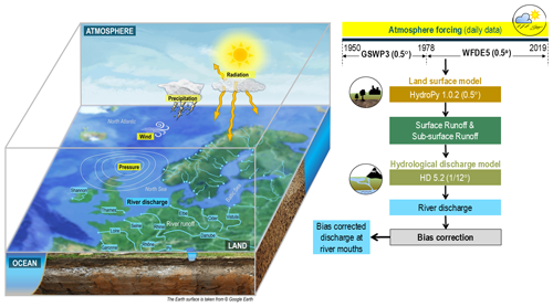
To generate the freshwater inflow from rivers to the ocean, we used an experimental setup analogous to Hagemann and Stacke (2022). Here we used two atmospheric forcing datasets (Sect. 2.1) and the same model chain of two large-scale hydrological models. The global hydrological model HydroPy (Sect. 2.2) was used to generate the input to the Hydrological Discharge (HD) model (Sect. 2.3) at the resolution of the atmospheric forcing data (0.5°). These input data of surface and subsurface runoff were then interpolated onto the HD model grid, and the HD model was used to simulate daily discharges from land to sea. Subsequently, we bias-corrected these time series as described in Sect. 2.4 to generate bias-corrected discharges at coastal ocean boxes of the European HD model domain from 1901–2019. Note that we combined the simulations based on two different atmospheric forcing datasets to cover the whole 20th century and to include the more recent years in the bias-corrected discharge time series. Such an approach was also used in the second phase (ISIMIP, 2023) of the Inter-Sectoral Impact Model Intercomparison Project (ISIMIP; Warszawski et al., 2014). Figure 1 summarises the experimental setup. Section 2.5 refers to the observational data that are used in the evaluation of the model results. Finally, the evaluation metrics used in the analysis of the results are presented in Sect. 2.7.

2.1 Atmospheric forcing

We used two atmospheric datasets comprising daily data of various near-surface atmospheric variables. They have been used as meteorological forcing datasets in several climate impact assessments and are recommended by ISIMIP (2023). Both datasets were specifically generated to force global hydrological models for hindcast simulations. They are based on re-analysis products from different weather forecast centres and bias correction procedures were applied by the respective creators to improve their data.

The Global Soil Wetness Project Phase 3 (GSWP3; Dirmeyer et al., 2006; Kim, 2017) dataset is available at 0.5° resolution from 1901–2014. To generate the GSWP3 dataset, Kim (2017) dynamically downscaled the 20th Century Reanalysis (Compo et al., 2011) onto the T248 (∼0.5°) grid using a spectral nudging technique (Yoshimura and Kanamitsu, 2008) in a global spectral model. Observation-based bias correction procedures were then applied to the downscaled data to obtain daily time series.

To generate the WFDE5 dataset, Cucchi et al. (2020) applied the WATCH Forcing Data methodology (Weedon et al., 2011) to surface meteorological variables from the ERA5 reanalysis (Hersbach et al., 2020) to obtain a bias-corrected time series. ERA5 is the fifth generation of atmospheric reanalysis produced by the European Centre for Medium-Range Weather Forecasts (ECMWF). WFDE5 is provided at 0.5° spatial resolution from 1979–2019. Mengel et al. (2021) stated that WFDE5 is considered the more realistic dataset, especially with respect to day-to-day variability for variables for which the monthly mean values were bias corrected, such as precipitation and temperature. For more information on application and evaluation of both datasets, see, e.g., Mengel et al. (2021) and references therein (Hassler and Lauer, 2021; Arora et al., 2023).

2.2 HydroPy setup

HydroPy (Stacke and Hagemann, 2021) is a state-of-the-art global hydrology model for which no model calibration was performed for its setup. Within global hydrological modelling, the usage of uncalibrated models is rather common (see, e.g., Haddeland et al., 2011), even though some models exist that are calibrated for global studies. In the present study, HydroPy was driven by daily forcing data from 1901–2019. Daily input fields of surface and subsurface runoff were generated at a resolution of 0.5°. Analogous to the ERA5 forced simulation in Hagemann and Stacke (2022), precipitation, 2 m temperature, downwelling shortwave and longwave radiation, 2 m specific humidity, surface pressure, and 10 m wind are used as forcing from the respective forcing dataset. We performed a spin-up simulation over 50 iterations of the year 1901 with the GSWP3 forcing (cf. Stacke and Hagemann, 2021) to initialise the storages in the HydroPy model and to avoid any drift during the actual simulation period. We then forced HydroPy with the GSWP3 data from 1901–1978 and continued with the WFDE5 data from 1979–2019. We also conducted a GSWP3 forced simulation from 1979–2014 in order to derive bias correction parameters for the earlier period. For our analysis, we focus on the years from 1950 onwards so that we have an additional transient spin-up of 49 years.

Figure 2 European HD model domain and catchment areas for selected rivers.

2.3 HD model setup

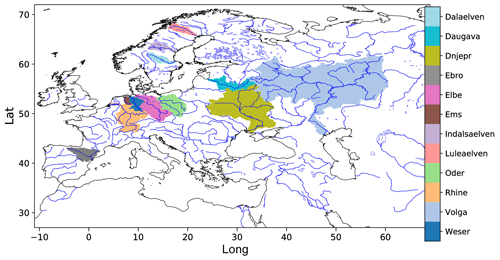
The HD model (Hagemann et al., 2020) is a well-established river-routing model that is implemented in a range of global and regional model systems. As noted in Hagemann et al. (2020), no river-specific parameter adjustments were conducted in the HD model to enable its applicability for climate change studies and over catchments where no daily discharges are available at a downstream station. To simulate discharge with the HD model, we used the daily input fields of surface and subsurface runoff that were generated by HydroPy from the GSWP3 and WFDE5 data (see Sect. 2.2). As the time step of these runoff data is 1 d, the time step of the HD model was also set to 1 d. However, an internal time step of 0.5 h is used for the flow within the river, as the minimum travel time through a grid box is limited by the chosen time step. The HD model v5.2.0 (Hagemann et al., 2023) was applied over the European domain, which covers the land areas between 27 to 72° N and −11° W to 69° E. The domain, along with a number of rivers specifically noted in this study, is shown in Fig. 2. In the following, we refer to the WFDE5-based discharges as HDW and to the GSWP3-based discharges as HDG. The corresponding bias-corrected discharges are referred to as HD-BC in general and HDW-BC and HDG-BC in particular.

Figure 3 Steps to derive bias-corrected discharge at river mouths from simulated discharges.

2.4 Bias correction of river runoff

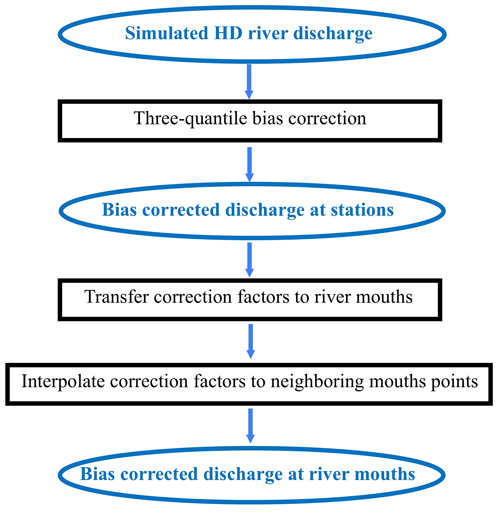
We have developed a bias correction method for river runoff that uses correction factors for three quantiles and includes a spatial transfer of these factors. We note that our three-quantile bias correction is similar to a very coarse quantile mapping. The latter has been introduced in climate change impact research to correct for significant biases in data produced by global and regional climate models. Quantile mapping is a distribution mapping in which the distribution function of climate values is corrected to match the observed distribution function. Details of such mapping applied to precipitation and surface air temperature can be found, for example, in Piani et al. (2010) and Teutschbein and Seibert (2012). Our bias correction method involves several steps. First, different correction factors for low, medium, and high percentiles are calculated at the station locations and then applied at the respective river mouths. Finally, an interpolation is performed on neighbouring coastal mouth points for which no downstream observations are available in the respective catchment. This procedure is summarised in Fig. 3. The three percentile ranges for daily discharge q_i are classified as

• low (L), q_i≤Q_p,

• medium (M), $Q_p<q_i<Q_{\mathrm{100}-p}$, and

• high (H), $q_i\ge Q_{\mathrm{100}-p}$.

Here, Q_p denotes the pth percentile of the daily discharge, and p was set to 20. The percentiles Q_p and Q_100−p were determined separately for the observed and the simulated discharges at the downstream station locations, and then the mean discharges $\stackrel{\mathrm{‾}}{q_R}$ were calculated for the three percentile ranges $R\in \left\{L,M,H\right\}$. Note that only those days for which an observed discharge was available were considered for these calculations. Then, the mean bias b_R (in %) was calculated for each percentile range, and a correction factor f_R to remove the bias was derived as

$$f_{\mathrm{R}}={\displaystyle \frac{\mathrm{100}}{b_R+\mathrm{100}}}.$$

For the evaluation of the bias correction in Sect. 3, these correction factors were applied to the simulated discharges at the station locations. As the correction factors are independent of the absolute amount of discharge, they could be applied to the respective river mouths. For each river mouth with more than one inflow (j>1) for which a correction factor f_R,j is determined, a combined correction factor is obtained by calculating an average weighted by the respective mean inflows Q_j.

$$\stackrel{\mathrm{‾}}{f_{\mathrm{R}}}={\displaystyle \frac{\sum _j{f}_{\mathrm{R},j}\times Q_j}{\sum _j{Q}_j}}$$

From these river mouths, an interpolation is performed on neighbouring coastal mouth points for which no downstream observations are available in the respective catchment. This interpolation was motivated by the fact that the general pattern of bias of neighbouring rivers is often similar (cf. Sect. 3.1). The interpolation is performed by inverse-distance weighting from the four (or fewer) closest river mouths within a search radius of 200 km. If no river mouth with a correction factor was found within the search radius, the correction factor was set to one (i.e. no correction).

Note that the bias correction can lead to spurious daily jumps in discharge when the percentile boundary is crossed and the bias correction factors differ between the percentile ranges. In order to reduce this effect, a smoothing radius of Δs=0.05 was introduced around the percentile boundaries, which was applied at both station locations and river mouths.

For $\left(\mathrm{1}-\mathrm{\Delta }s\right)\times Q_p<q_i<\left(\mathrm{1}+\mathrm{\Delta }s\right)\times Q_p$,

$$\stackrel{\mathrm{̃}}{q_i}=q_i\times (f_L+\left(f_M-f_L\right)\times {\displaystyle \frac{(q_i-\left(\mathrm{1}-\mathrm{\Delta }s\right)\times Q_p)}{\mathrm{2}\times \mathrm{\Delta }s\times Q_p}}.$$

For $\left(\mathrm{1}-\mathrm{\Delta }s\right)\times Q_{\mathrm{100}-p}<q_i<\left(\mathrm{1}+\mathrm{\Delta }s\right)\times Q_{\mathrm{100}-p}$,

$$\stackrel{\mathrm{̃}}{q_i}=q_i\times (f_M+\left(f_H-f_M\right)\times {\displaystyle \frac{(q_i-\left(\mathrm{1}-\mathrm{\Delta }s\right)\times Q_{\mathrm{100}-p})}{\mathrm{2}\times \mathrm{\Delta }s\times Q_{\mathrm{100}-p}}}.$$

The bias correction procedure corrects the days that fall into the different percentile ranges. However, this does not necessarily mean that it also corrects the whole distribution into the three percentile ranges. Particularly if the biases in these ranges are quite different, the days may change their class and order within the distribution.

In order to apply the three-quantile bias correction to the simulated discharge time series from 1901–2019, two sets of bias correction factors were derived. The first set uses HDW and discharge station observations for the period 1979–2014. This set was used to bias correct the simulated discharge at HD river mouths from 1979–2019. The second set uses a further discharge simulation, where we continued HDG and utilised the GSWP3 forcing up to 2014. Again, the set of bias correction factors was derived for the period 1979–2014 using discharge station observations. This set was then used to bias correct the simulated discharge at the HD river mouths from 1901–1978.

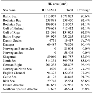
Table 1 Sea basin catchment areas on the HD model grid and the fractional catchment coverage of the associated IGC-EMO rivers. Fractional coverages of less than 75 % are indicated in italic.

Table 2 Country catchment coverage of OSPAR data and inclusion of estimates for unmonitored areas (Borgvang et al., 2008). NI means that no information on the coverage was provided.

¹ Only for the Eider river. ² A total of 10 % in direct discharge. ³ For example, Farkas and Skarbøvik (2021).

Figure 4 Selected HELCOM (a) and OSPAR (b) basins for which inflows are considered. For OSPAR, the Spanish Atlantic basin is limited to the coast of northern Spain.

2.5 Observed discharge data

We used available daily discharge data from downstream gauges for many rivers across Europe with a catchment area of about 1000 km² or more. These station data were obtained from Global Runoff Data Centre and various agencies and institutions listed in Table 2 of Hagemann and Stacke (2022). In addition, French discharge data were accessed from the EU Copernicus Marine Service Information. In order to allow an assessment of the discharge at the river mouths, we considered basin-wide estimates from three different sources.

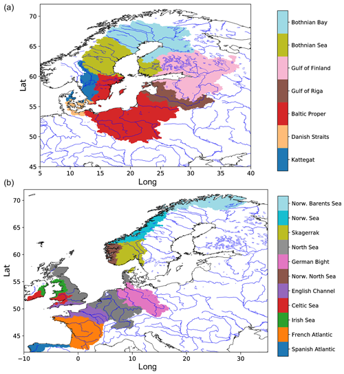
For the Baltic Marine Environment Protection Commission, also known as the Helsinki Commission (HELCOM), Svendsen and Gustafsson (2022) provided annual waterborne inflows into the seven main sub-basins of the Baltic Sea (Fig. 4; upper panel) from 1995 to 2020. Waterborne inflows comprise the sum of river runoff and direct inflows, i.e. flows from point sources discharging directly into the Baltic Sea. These point sources are not included in our experimental setup or in the bias correction. However, their contribution to the total waterborne inflow to the Baltic Sea is only about 1 % (HELCOM, 1998).

Under the umbrella of the OSPAR Convention (Convention for the Protection of the Marine Environment of the northeast Atlantic), the IGC-EMO (Intersessional Correspondence Group for Eutrophication Modelling) database (Lenhart et al., 2010) of daily riverine freshwater inflows and nutrient loads was compiled by Van Leeuwen and Lenhart (2021), covering the major rivers discharging into the Baltic Sea, the North Sea, and the northeast Atlantic. An updated database covering a total of 370 rivers was mapped onto the flow grid of the European $\mathrm{1}/\mathrm{12}\mathit{°}$ domain of the HD model by Van Leeuwen and Hagemann (2023). The associated catchment areas of these rivers, which flow into a particular specific sea basin, do not cover the entire catchment area of the respective basin (see Table 1), so the total inflow of the sea basin is underrepresented by the IGC-EMO data. To generate basin-wide estimates, we have up-scaled these values by dividing the integrated IGC-EMO river discharges in a basin by the fractional coverage of the entire basin catchment on the HD grid. Basin estimates for which the fractional coverage is less than 75 % are considered to be highly uncertain and are therefore provided for completeness only but are not included in the assessment of simulated inflows.

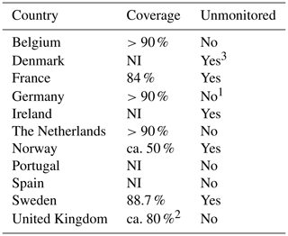
In addition, we used estimates of long-term mean sub-basin-wide inflows to the North Sea and northeast Atlantic that were published by OSPAR (Farkas and Skarbøvik, 2021). Figure 4 (lower panel) shows the selected OSPAR basins for which the inflows are considered. It should be noted that the sea basin inflows provided by the different OSPAR countries are not consistent. Some countries include discharge estimates for unmonitored areas, while others do not (Table 2). In addition, the sea basin catchment coverage of the monitored areas varies between the countries. Note also that we have excluded the Spanish Atlantic from our comparisons for the following reason. Here, we limited the Spanish Atlantic basin to the coast of northern Spain (see Fig. 4; lower panel) to allow a comparison with the IGC-EMO data, as the IGC-EMO data only cover rivers in this region, hereafter referred to as NSpA. These rivers cover about 38 % of the total NSpA area on the HD model grid (Table 1), while the OSPAR data for NSpA cover about 50 % (23 201 km²; Farkas and Skarbøvik, 2021). However, the associated IGC-EMO discharge from 1961–1990 (629 m³ s⁻¹) is 75 % larger than the OSPAR long-term mean average (359 m³ s⁻¹). Therefore, both inflow values are unlikely to be representative of the NSpA region, and this region is not considered in the following.

2.6 Ocean model experiments

To assess the effect of using bias-corrected river discharge on simulated salinity in the German Bight, we used version 3.6 of the Nucleus for European Modelling of the Ocean (NEMO; Madec et al., 2017) and adopted a domain setup used by Ho-Hagemann et al. (2020). This domain covers the region of the northwest European shelf, the North Sea, and the Baltic Sea between 40.07 to 65.93° N and 19.89 to 30.16° E with a resolution of 2 nautical miles (ca. 3.6 km). We used the atmospheric forcing from ERA5 and the ocean boundary forcing from the ECMWF Ocean Reanalysis System 5 (ORAS5; Zuo et al., 2019) to conduct two simulations from 2010 to 2018. Initial conditions were taken from a 20-year spin-up simulation driven by ERA5 data, so that the deeper ocean layers could adapt to the present-day climate (Sebastian Grayek, personal communication, 2023). Note that for the evaluation of results, we neglected the year 2010 to have an additional spin-up in which NEMO could adapt to the specific transient conditions within each of the two experiments. For the German Bight, this spin-up of 1 year is sufficient, as the residence time of water may comprise only up to 4 months (Becker et al., 1999). In the two experiments, the daily riverine inflow into the ocean was taken from the uncorrected and bias-corrected discharges of HDW, which were converted to the NEMO grid using a procedure of Nguyen et al. (2024). For each HD model river mouth box, we associated the nearest coastal ocean box on the NEMO grid if such a box was found within a search radius of 200 km. Such a large radius is necessary because the NEMO coastline is very smooth, so many estuaries and bays in the HD model grid are not resolved by NEMO. If no ocean box was found, the corresponding HD model box was not linked. Consequently, the simulated discharge data at the river mouths were placed as freshwater inflow into the corresponding NEMO grid boxes.

2.7 Evaluation metrics

The evaluation of the simulated discharge was performed for the grid boxes corresponding to the discharge station locations within the river network. For the evaluation at these station locations, we used the mean bias, the Pearson correlation coefficient, and the Kling–Gupta efficiency (KGE; Gupta et al., 2009; Kling et al., 2012). All metrics were calculated with simulated and observed daily discharge time series for the period considered, using only those days for which observed data are available. The KGE is a quality metric combining the bias, correlation, and coefficient of variation. If a simulated discharge time series has a KGE $>-\mathrm{0.41}$, then it is a better representation of the observations than the use of the observed long-term mean discharge (Knoben et al., 2019). Note that many ocean model applications still use the latter method.

For the evaluation of simulated salinity in the NEMO experiments, we used daily values and considered

• the mean bias

• the correlation of simulated and observed time series expressed by the Pearson correlation coefficient

• the variability ratio defined by the ratio of the simulated and observed coefficients of variation

• the normalised root mean square error (RSME)

• the centred RSME.

The first four metrics are described, e.g. ,in Hagemann et al. (2020), while the centred RSME is described, e.g., in Taylor (2001).

Figure 5 Mean discharge bias [%] (a, b) and KGE (c, d) for HDG (a, c) and HDW (b, d) during 1979–2014.

3 Evaluation of the bias correction

Below, various metrics have been calculated at the station locations and at the river mouths. However, these measures have been assigned to the respective catchment areas for the purpose of graphical presentation.

3.1 Evaluation of simulated discharge

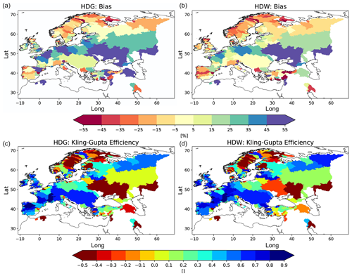
The distribution of bias and KGE for HDG and HDW during 1979–2014 (Fig. 5) is quite similar to the pattern shown by Hagemann and Stacke (2022) for the ERA5-based discharge. For both simulations, the general discharge behaviour is well captured (KGE >0.4) for many European rivers, especially in northern Iberia, western and central Europe, and over northern Russia (Fig. 5; lower row). As expected (cf. Hagemann et al., 2020), larger deviations in the simulated from observed discharges occur for rivers that are heavily influenced by human activities such as water abstraction, e.g., for irrigation, and regulation, e.g., by dams. This is the case for many Scandinavian and Turkish rivers, as well as the Volga and Don.

In general, the HDW discharges are slightly drier than the HDG discharges, as indicated by larger dry biases in northern Europe and smaller wet biases in central Europe. Despite the differences in bias distribution, the KGEs of HDW are similar to or slightly better than those of HDG. Compared to the ERA5-based discharge of Hagemann and Stacke (2022), HDW tends to have smaller discharge biases and better KGEs. This is an expected behaviour caused by the application of a bias correction methodology to the ERA5 data in the generation of the WFDE5 data (cf. Sect. 2.1). An exception to this general improvement occurs over northern Europe, where the dry bias of HDW tends to be slightly larger and the KGEs lower. Note that Hagemann and Stacke (2022) attributed the dry bias over northern Europe to an overestimation of the evapotranspiration simulated by HydroPy.

We also note the large-scale patterns of positive and negative discharge biases (Fig. 5). Abrupt changes in bias behaviour along the same coastline are rare. Most of the few cases can be attributed to large human water abstractions from the river, i.e. especially for the Ebro river (see also Sect. 3.3) and in the Republic of Türkiye, which are not considered by the model. This supports our assumption about the spatial transferability of the three-quantile bias correction factors. The bias patterns are related to biases in the atmospheric forcing dataset or biases introduced by the HydroPy model.

In order to analyse how much the bias correction affects the daily sequence of river runoff at the station locations, we calculated the correlation between the simulated discharges and the observations. Figure S1 in the Supplement shows that the correlation patterns of HDW and HDW-BC with observed discharges are quite similar. For rivers where differences can be identified, the correlation mostly increases for HDW-BC. The correlation between HDW and HDW-BC is generally higher than 0.95, and only a very few rivers show correlations lower than 0.9. These rivers are usually rivers that are heavily influenced by human activities, such as the Volga and the Luleälven.

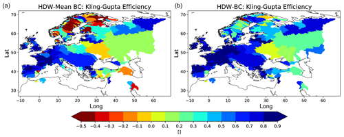
Figure 6 KGE for bias-corrected HDW discharges using the mean bias correction (a) and the three-quantile bias correction (b) during 1979–2014.

Table 3 Mean bias and KGE of simulated (HDW) and bias-corrected discharge during 1979–2014 for selected rivers, where the three-quantile bias correction led to a noticeable KGE improvement in comparison to the mean bias correction.

3.2 Added value of the three-quantile bias correction

In this section, we consider the effect of the bias correction at the station locations and investigate whether the three-quantile bias correction adds value compared to using only the mean bias correction. For this purpose, we use HDW and the period 1979–2014.

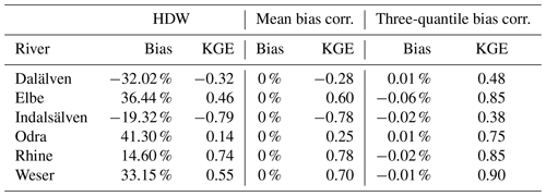
Both bias correction methods reduce the mean discharge bias to zero or close to zero in the case of the three-quantile bias correction due to the smoothing around the percentile range thresholds (see Table 3 for selected rivers). When the mean bias correction is applied, the KGEs (Fig. 6; left panel) are noticeably improved over western and central Europe. However, with a few exceptions, the KGE pattern over northern Europe and other areas remains largely unchanged. This indicates that a correction of the long-term bias in the annual mean discharge over these areas is not sufficient. Only with the three-quantile bias correction does the KGE (Fig. 6, right panel; see Table 3 for selected rivers) improve considerably over these areas, with the largest improvements occurring over Scandinavia. The three-quantile bias correction also leads to some further improvements over western and central Europe, where the bias-corrected discharge with the mean bias correction already shows relatively high KGE values, e.g., for the rivers Elbe, Rhine, and Weser.

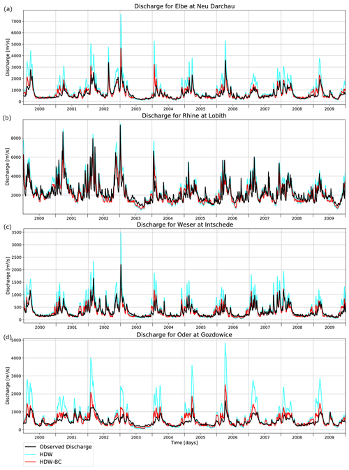
Figure 7 Observed and simulated daily discharges for the rivers (a) Elbe, (b) Rhine, (c) Weser and (d) Odra during 2000–2009.

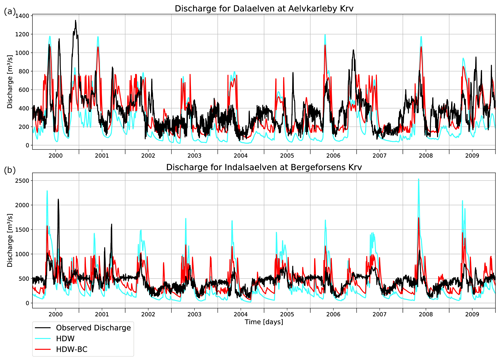
Figure 8 Observed and simulated daily discharges for the rivers (a) Dalälven and (b) Indalsälven during 2000–2009.

To visualise the effect of the three-quantile bias correction on the simulated daily discharges, we consider the corresponding discharge curves for the period 2000–2009 for selected large rivers. The respective biases and KGE are shown in Table 3 for the period 1979–2014. For the rivers Elbe, Weser, and Oder, the peak discharges are generally overestimated, while the low flows are close to the observed values (Fig. 7a, c, d). The correction of the high percentiles leads to a considerable improvement in the representation of the peak discharges, while the change in the low flows is rather small. The discharge of the Rhine (Fig. 7b) is well represented by HDW. However, the small downward correction of the peak discharges and the slight increase in the low flows still lead to an improved discharge curve, which is also indicated by the increased KGE (Table 3).

As mentioned above, the greatest improvements from the three-quantile bias correction compared to the application of the mean bias correction occur over Scandinavia. Here many rivers are highly regulated. For this reason, the discharge curves of the Dalälven and Indalsälven rivers are examined in more detail in Fig. 8. The observed discharges clearly show the effect of the human regulation, where regulation leads to the elimination of peak discharges, while maintaining certain flows during low-flow periods. Figure 8 shows that, on the one hand, peak discharges are often suppressed or reduced, especially during the spring, and that, on the other hand, low-flow periods are either almost absent (especially for the Indalsälven) or show a rather noisy and unnatural daily variability. Here, the bias correction partially mimics these regulation effects by reducing the peak discharges and increasing the low flows.

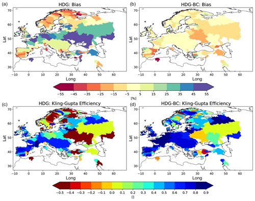
Figure 9 Mean discharge bias [%] (a, b) and KGE (c, d) for HDG (a, c) and HDG-BC data (b, d) during 1950–1978.

Figure 10 Observed and simulated daily discharge based on HDG for the Ebro river during (a) 1960–1969 and (b) 2000–2009.

3.3 Application of the bias correction for a different time period

To consider the effect of the bias correction for the applications over different time periods, we derived bias correction factors for HDG during 1979–2014 and applied the factors for the period 1950–1978.

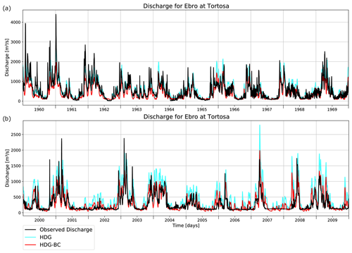
For HDG, the distributions of bias and KGE are quite similar between the two periods 1950–1978 (Fig. 9; left column) and 1979–2014 (Fig. 5; left column). Consequently, the bias correction leads to improvements in the KGE (Fig. 9) that are similar for the most recent period (not shown). The bias also becomes less for most of the rivers. Noticeable exceptions are the Dnipro, Volga, and some rivers in southern Europe. This may be related to differences in the anthropogenic influence on the discharge between the two periods, as is the case for the river Ebro. Here, the large wet bias (51.65 %) in the more recent period is contrasted with a small wet bias (12.05 %) in the earlier period (Fig. 10). Since large anthropogenic water abstractions occur in the Ebro river (Merchán et al., 2013), this seems to be related to the different irrigation activities in the two periods, which are much more pronounced in more recent years. The latter can be seen by looking at the observed daily discharges between 1960–1969 and 2000–2009 (Fig. 10). In the earlier period, the Ebro discharge still shows some variations according to the sequence of weather events in the dry season. However, in the later period, the observed discharge includes only very small variations during the dry season, indicating more intense human water abstraction than in the earlier period. Consequently, the bias correction based on the recent wet bias leads to a dry bias (−25.78 %) in the corrected Ebro discharge in the earlier period. However, the KGE decreases only slightly from 0.68 to 0.63, so that the deterioration of the mean bias seems to be largely compensated by the correction of the different percentile ranges.

Figure 11 Trends in annual maximum (a, b), mean (c, d), and minimum (e, f) discharge [% yr⁻¹] for HDW (a, c, e) and HDW-BC (b, d, f) from 1979–2014.

3.4 Effect of the bias correction on contemporary trends

As mentioned in Sect. 2.4, our three-quantile bias correction is similar to a very coarse quantile mapping, and quantile mapping has been flagged as potentially not suitable for climate simulations, as it has been shown to modify trends (e.g. references in Cannon et al., 2015). However, Maraun et al. (2017) pointed out that a debate has arisen about whether trend modification by variance-adjusting bias correction methods actually improves or degrades the raw climate change signal. They further argued that purely statistical arguments cannot resolve this issue, which requires process understanding. With respect to runoff, the latter needs to take into account spatial and temporal characteristics of rivers and events, which is beyond the scope of the present large-scale study.

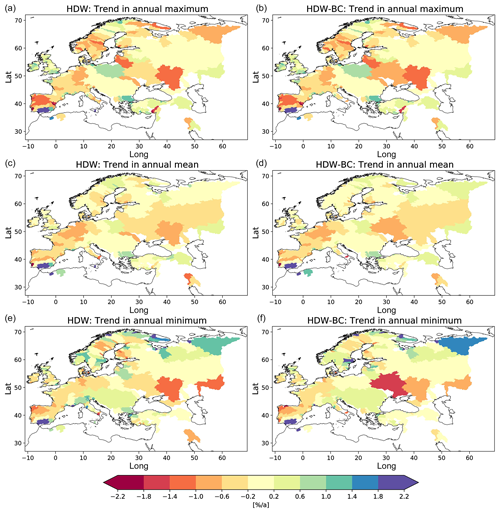
To investigate the effect of the bias correction on contemporary trends, we calculated trends in the annual maximum, mean, and minimum discharge for the period 1979–2014 and compared the results for HDW and HDW-BC (Fig. 11). The trend patterns are generally within the range spanned by the two datasets considered in Hagemann and Stacke (2022). For the annual maximum and mean discharge, the trend patterns are only slightly changed by the bias correction. For the annual minimum discharge, the trend pattern is quite similar in HDW and HDW-BC. However, there are a few more rivers where the magnitude of the trend is affected by the bias correction. This is particularly the case over Scandinavia, where many rivers are regulated, so that the correction of the low-percentile range is often strong to account for the effect of regulation on low flows (cf. Sect. 3.2).

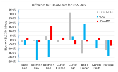
Figure 12 Relative difference in basin inflows compared to HELCOM data for 1995–2019. Note that no IGC-EMO estimate is provided for the Danish Straits as the respective river catchment coverage in IGC-EMO is too small.

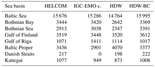
Table 4 Estimated and simulated inflows (units in m³ s⁻¹) into the Baltic Sea and its major sub-basins during 1995–2019. Note that for the Danish Straits no IGC-EMO estimate is provided as the respective catchment area coverage of the rivers in IGC-EMO is too low. Note that “IGC-EMO c.” stands for the IGC-EMO catchment.

4 Evaluation of the inflow into sea basins

To evaluate the simulated and bias-corrected discharges at the river mouths, we considered the integrated inflow into different sea basins. First, we evaluated the discharges into the Baltic Sea using HELCOM and IGC-EMO data in Sect. 4.1. We then compared the discharges to the North Sea and the northeast Atlantic with OSPAR and up-scaled (see Sect. 2.5) IGC-EMO data in Sect. 4.2.

4.1 Baltic Sea

In order to achieve a maximum overlap of the simulated discharge time series data with the HELCOM data (cf. Sect. 2.5), we considered 1995–2019 as the evaluation period for the Baltic Sea and its seven sub-basins (Fig. 4; upper panel). For the whole Baltic Sea and most of its sub-basins, the bias correction improves the basin inflows if compared to the HELCOM estimates (Table 4; Fig. 12). Only for the Gulf of Finland and the Gulf of Riga does the bias correction leads to a slightly larger bias, while the biases of HDW in these basins are relatively small. When the simulated inflows are compared with the IGC-EMO estimates, similar results are obtained, except for the Gulf of Riga. Here, the IGC-EMO estimates are about 32 % larger than the HELCOM estimates, indicating a larger uncertainty in at least one of these two estimates. For the Gulf of Riga basin, the major part of the inflow is contributed by the Daugava River. In IGC-EMO, the discharge from the Daugava is based on observed time series from 1970–1990. These data were extended to earlier and later periods, e.g., by climatological values and trend preservation (Van Leeuwen and Hagemann, 2023). For 1970–1990, the mean IGC-EMO discharge comprises 623 m³ s⁻¹ at the Daugava mouth, while this has increased by ca. 45 % in 1995–2019 (902 m³ s⁻¹). However, this strong increase cannot be seen in the observed discharge time series at the station Daugavpils that covers about three-quarters of the Daugava catchment. Here, the discharge increases only slightly from 1970–1999 (439 m³ s⁻¹; 95 % temporal data coverage) to 1995–2019 (452 m³ s⁻¹; 83 % temporal data coverage). This indicates a large overestimation of the IGC-EMO Daugava discharge during 1995–2019 and, hence, also of the respective Gulf of Riga inflow.

Figure 13 Relative difference in basin inflows compared to OSPAR data for 1961–1990. IGC-EMO basin estimates for which the fractional catchment coverage (see Table 1) is less than 75 % are not shown.

4.2 North Sea and northeast Atlantic

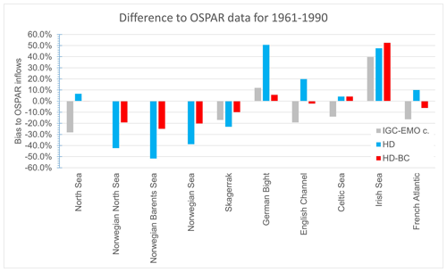
Due to the different treatment of unmonitored regions by the OSPAR countries (cf. Sect. 2.5), and thus of the respective sea basin areas, we have not corrected the OSPAR inflows. Instead, we have also considered up-scaled IGC-EMO data as alternative estimates of basin inflow (as in Sect. 4.1). Table 5 shows simulated and estimated basin inflows for the considered OSPAR regions (cf. Fig. 4; lower panel). Note that IGC-EMO data for the Norwegian shares of the Barents Sea, Norwegian Sea, and North Sea and the north Spanish Atlantic are not included in the following comparisons due to their limited area coverage. When comparing the simulated sea basin inflows with the OSPAR and IGC-EMO data, we found that the bias correction improves the simulated inflows for most of the OSPAR regions (Fig. 13). Exceptions are the values for the Celtic Sea and the Irish Sea. For the Celtic Sea, the bias-corrected inflows are very close to the uncorrected inflows, and the difference with the OSPAR data is rather small. For the Irish Sea, the bias-corrected inflows are somewhat larger than the uncorrected ones, with both showing large differences (52.5 % and 47.5 %) compared to the OSPAR data. Here both inflows are closer to the IGC-EMO estimate, which exceeds the OSPAR estimate by about 40 %.

Table 5 Estimated and simulated inflows (units in m³ s⁻¹) into major sub-basins of the North Sea and the northwest Atlantic during 1961–1990. Note that the North Sea does not comprise Skagerrak and the English Channel. Up-scaled IGC-EMO basin estimates for which the fractional catchment coverage (see Table 1) of IGC-EMO rivers is less than 75 % are considered highly uncertain and are therefore only given in parentheses (cf. Sect. 2.5). The same applies to the OSPAR inflow into the northern Spanish Atlantic.

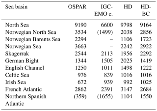
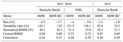
Table 6 Various metrics (see Sect. 2.7) of the simulated salinity time series at 6 m depth compared with the observations at the stations of Deutsche Bucht and EMS for 2011–2018 and at Deutsche Bucht for 2013.

While the OSPAR values from Ireland include estimates for unmonitored areas, this is not the case for the United Kingdom (Table 2). Farkas and Skarbøvik (2021) list the rivers contributing to the OSPAR value (560 m³ s⁻¹) from the United Kingdom part of the Irish Sea catchment (35 000 km²). Adding up the catchment areas of each river, obtained from various online resources, gives a coverage of about 70 %. In order to account for this under-representation of the catchment area, an up-scaling can be performed, similar to the treatment of the IGC-EMO data. This would give an estimate of about 803 m³ s⁻¹ for the Irish Sea inflow from the United Kingdom and thus 915 m³ s⁻¹ for the whole Irish Sea. The respective IGC-EMO inflow is close to this value (+2.6 %), and the overestimation of inflows is less pronounced for HD and bias-corrected discharges with +8.4 % and +12 %, respectively.

Figure 14 Mean analysed SSS in (a) Droghei et al. (2018) data (OBS) and various SSS differences in the NEMO experiments in the German Bight for the period from 2010 to 2018. The SSS differences comprise (b) HD-BC minus HDW, (c) HDW minus OBS, and (d) HD-BC minus OBS.

4.3 Simulated salinity in the German Bight

Using the two experiments described in Sect. 2.6, we evaluated the simulated sea surface salinity (SSS) with satellite-based analyses and in situ observations for the period 2010 to 2018. The SSS analyses were derived using a multivariate optimal interpolation algorithm that combines sea surface salinity images from several satellite sources, such as the National Aeronautics and Space Administration Soil Moisture Active Passive satellite and the European Space Agency Soil Moisture and Ocean Salinity satellite, with in situ salinity measurements (Droghei et al., 2018). These SSS data are available with a spatial resolution of 0.125°.

Figure 15 Coefficients of variation in SSS in the German Bight for the period from 2011–2018. (a) OBS, (b) HDW, and (c) HD-BC.

Figure 16 Observed (OBS) and simulated daily time series of salinity in 6 m depth for the stations (a) Deutsche Bucht (DB) and (b) EMS (units in PSU). The solid blue and red lines correspond to the HDW and HD-BC experiments, respectively. The green line separates the spin-up period in 2010 from the evaluation period 2011–2018.

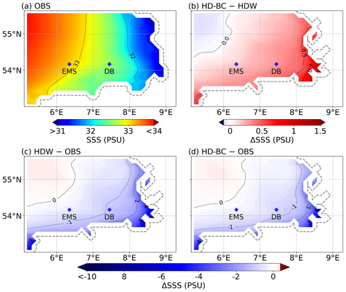
Figure 14a shows the mean analysed SSS in the German Bight for the period 2010–2018, with lower salinities near the west coast of Germany and higher salinities towards the east. The NEMO simulation using the uncorrected discharges of HDW (Fig. 14c) has SSS that is too low in coastal areas, especially near the estuaries. This low bias is reduced using the bias-corrected discharges (Fig. 14d), as the general effect of the bias correction in the German Bight leads to reduced riverine inflows (cf. Fig. 13) and hence increased SSS in coastal areas (Fig. 14b). Similar improvements can also be seen in June 2013 when the Elbe flood is strongly influences the SSS of the German Bight (Fig. S2). Here, the increase in salinity due to the bias-corrected runoff (Fig. S2b) is more pronounced than in the long-term mean (Fig. 14b). In addition, we found that use of the bias-corrected river runoff also improves the SSS variability expressed by its coefficient of variation, as shown in Fig. 15.

In addition, we had access to salinity measurements at two stations in the German Bight operated by the German Federal Maritime and Hydrographic Agency as part of the Marine Environmental Monitoring Network in the North and Baltic seas. These two stations are Deutsche Bucht (DB; located at 54.17° N, 7.45° E) and EMS (54.17° N, 6.35° E), and their locations are shown in Fig. 14. In general, the bias-corrected discharges lead to improved characteristics of the daily salinity at 6 m depth at the Deutsche Bucht and EMS stations (Fig. 16; Table 6). Here the bias and normalised and centred RSME are decreased, and the coefficient of variation is closer to the salinity observations for HDW-BC. This means that the bias correction improves the mean and the variability in the simulated salinity at these stations. However, the correlation with the observed salinity measurements is somewhat reduced. Note that temporal SSS variations are strongly influenced by local currents, vertical mixing, and wind–wave–surface interactions. Therefore, signals from an improved river runoff can easily be obscured by the noise from these processes, which can also differ at the point scale of the station measurements and at the grid scale of the respective NEMO grid box. This is reflected in the relatively low correlation values. Furthermore, this can be seen when the gridded SSS data of Droghei et al. (2018) are used as a reference for the metrics at the station locations (Table S1 in the Supplement). Here, all metrics improve with HDW-BC, even the correlation. However, the correlation is lower than with the station observations, which is also the case for the correlation of the gridded SSS data with the station observations (Deutsche Bucht: 0.15; EMS: 0.18). Considering only the year 2013, when the influence of the Elbe flood on the salinity at the Deutsche Bucht station is more pronounced (Nguyen et al., 2024), the correlation also improves when using HDW-BC for both references (Tables 6 and S1). It seems that in NEMO the positive effect of using bias-corrected discharges is limited to near-surface salinities, as there is no noticeable effect at 30 m depth (not shown). This is consistent with the fact that the Deutsche Bucht and EMS stations are located in an area where the salinity is temporarily stratified, depending on the meteorological conditions and the intensity of river runoff (Klein and Frohse, 2008).

In summary, the results of the NEMO experiments indicate the beneficial effect of using bias-corrected discharges on the simulated SSS in coastal areas. However, although the low SSS biases are reduced using the bias-corrected discharges, the simulated SSS is still underestimated in coastal areas, especially close to the estuaries of large rivers (Fig. 14d). This may be attributed to the rather smooth coastline of the NEMO ocean grid. Here, most parts of the large estuaries of the rivers Elbe, Ems, and Weser are not included. In reality, a major part of the mixing of the riverine freshwater inflow and the saline North Sea happens within these estuaries. In the NEMO model setup, the freshwater inflow is introduced at the respective river mouth points of the smooth NEMO coastline where it starts to mix with the saline North Sea water. Consequently, the simulated water at and near those points is much fresher than in reality, which leads to the low SSS bias. Note that, on the one hand, such a smooth coastline is necessary in NEMO to avoid numerical instabilities. On the other hand, the spatial resolution of the NEMO grid is not high enough to adequately resolve parts of the longer estuaries.

5 Summary and conclusions

In the present study, we have introduced a methodology for the bias correction of European river runoff to provide corrected riverine inflows as forcing for ocean models in offline and coupled system model simulations. The central part of this methodology is a three-quantile bias correction, which can correct different biases for low, medium, and high discharges. The bias correction parameters are derived in two steps. First, different correction factors for low, medium, and high flows are derived for each river considered (cf. Sect. 2.5) at the location of the most downstream station for which daily discharge measurements were available. These factors were then transferred to the respective river mouth on the HD model grid and to adjacent coastal inflow points in its vicinity.

The evaluation of the bias-corrected discharge at the station location showed that the bias correction greatly improved the simulated discharges. For the evaluation of the bias-corrected discharge at the downstream station locations, we considered the mean bias and the KGE, which is a quality metric combining the bias, correlation, and coefficient of variation. Considering the same period as used to derive the bias correction factors, the mean bias is trivially close to zero. However, the bias is also substantially reduced for most rivers if a different period is considered. Irrespective of the period, the KGE pattern generally improves for the bias-corrected discharges and shows high values for many rivers. Exceptions are those rivers with a very strong anthropogenic distortion of the natural flow, e.g. by many dams or large water withdrawals. Here, despite some improvements, the KGE values are still rather low, such as for the rivers Dnipro, Volga, Luleälven, and a few Turkish rivers flowing into the Black Sea. The KGE also shows the beneficial effect of the three-quantile bias correction, as correcting only the long-term mean annual discharge bias is not sufficient in many areas, especially in northern Europe. We found that the three-quantile bias correction often improves the KGE in regulated rivers, so that it appears to mimic the effect of regulation, where regulation leads to the elimination of peak flows while maintaining certain flow levels during low-flow periods.

The evaluation of riverine inflows to the sea at river mouths with observed daily discharge is rarely possible as there are usually no river gauges available. Even if there is a gauge at the mouth of a river, the measurements are often affected by tidal influences from the coast, so that the measured amounts may not represent the actual river discharge. For obvious reasons, it is also difficult to compare simulated inflows with observed discharges for unmonitored rivers. Therefore, we compared the simulated and bias-corrected discharges with long-term mean inflow estimates into different sea basins from HELCOM, OSPAR, and IGC-EMO. For most of the basins considered, the bias correction improves the simulated inflows. This indicates a reasonable performance of the approach to transfer the bias correction factors obtained at the downstream stations to the respective river mouths and adjacent coastal areas. The improved inflows to the sea basins, together with the fact that the discharge bias behaviour tends not to vary abruptly along the same coastline, underpin the validity of our transferability approach. Exceptions are the Gulf of Finland, the Gulf of Riga, the Celtic Sea, and the Irish Sea. For the Gulf of Finland and the Celtic Sea, the deviations of the uncorrected and bias-corrected inflows from the inflow estimates are rather small. For the Gulf of Riga, the deviations of the uncorrected and bias-corrected inflows from the HELCOM estimates are also small, but they significantly underestimate the IGC-EMO estimates. However, this could be due to a large overestimation of the Daugava discharge during the period 1995–2019 in the IGC-EMO data and thus also of the corresponding Gulf of Riga inflow. For the Irish Sea, IGC-EMO seems to be closer to reality as the OSPAR inflow does not cover the unmonitored rivers in the British part of the catchment.

A caveat applies for rivers where the human influence on river flow has changed significantly over time. Applying bias correction factors derived for 1979–2014 to earlier periods may lead to errors for regulated rivers in years before these regulatory measures were implemented. This is the case for the Ebro, where irrigation activities have largely intensified during the period 1979–2014 compared to earlier periods (see Sect. 3.3). A detailed analysis of the rivers and periods concerned is beyond the scope of this study. However, at least for the period 1950–1978, the KGE distribution does not seem to be significantly affected, as there is no noticeable deterioration.

We have shown that our bias correction method works well for Europe at the station locations, as well as for the riverine inflow into northern and western European sea basins. Using two NEMO simulations in the German Bight, we have also shown that the use of the bias-corrected discharges as forcing leads to an improved simulation of sea surface salinity in coastal areas, especially regarding the mean salinity and its variability. However, for the potential transfer of the bias correction methodology to other regions, it has to be pointed out that the application of the three-quantile bias correction over a region only makes sense if a large part of the catchment area is covered by available daily discharge measurements. As the three-quantile bias correction is based on biases in three percentile ranges of daily flows, it is also suitable for the use in climate change applications. Here the bias correction factors can be derived from a historical discharge simulation and then applied to future projections or past reconstructions. In addition, the bias correction can also be applied in regional coupled system model simulations, where the bias correction factors can be derived from an initial simulation and then applied during the runtime of the actual coupled simulation. This capability has been implemented in the HD model v5.2.2 (Hagemann et al., 2023) and is currently being applied in the coupled system model GCOAST-AHOI (Ho-Hagemann et al., 2020). Finally, we note that the bias-corrected discharges are available from the World Data Centre for Climate and are already used within the CoastalFutures project (https://www.coastalfutures.de, last access: 7 November 2024).