Predicting particle catchment areas of deep-ocean sediment traps using machine learning

The ocean's biological carbon pump plays a major role in climate and biogeochemical cycles. Photosynthesis at the surface produces particles that are exported to the deep ocean by gravity. Sediment traps, which measure deep-carbon fluxes, help to quantify the carbon stored by this process. However, it is challenging to precisely identify the surface origin of particles trapped thousands of meters deep due to the influence of ocean circulation on the sinking path of carbon. In this study, we conducted a series of numerical Lagrangian experiments in the Porcupine Abyssal Plain region of the North Atlantic and developed a machine learning approach to predict the surface origin of particles trapped in a deep-ocean sediment trap. Our numerical experiments support the predictive performance of the machine learning approach, and surface conditions appear to provide valuable information for accurately predicting the source area, suggesting a potential application with satellite data. We also identify factors that potentially affect prediction efficiency, and we show that the best predictions are associated with low kinetic energy and the presence of mesoscale eddies above the trap. This new tool could provide a better link between satellite-derived sea surface observations and deep-ocean sediment trap measurements, ultimately improving our understanding of the biological-carbon-pump mechanism.

1 Introduction

The biological carbon pump (BCP) plays a major role in climate and biogeochemical cycles. The BCP reduces unperturbed atmospheric CO₂ by 35 % to 50 % (Williams and Follows, 2011) by exporting organic matter to the deep ocean, thereby supporting abyssal food webs (Billett et al., 1983; Rembauville et al., 2018). The BCP is driven by photosynthesis that occurs within the euphotic layer, typically between 0 and 200 m, producing gravitationally sinking particulate organic carbon (POC). Sinking particles have a wide range of vertical velocities, from neutral buoyancy to more than 600 m d⁻¹ (Villa-Alfageme et al., 2016), and are usually considered the main contributors to the BCP (Armstrong et al., 2001; Alonso-González et al., 2010; Siegel et al., 2014; Le Moigne, 2019). While most POC is remineralized in the euphotic and mesopelagic zones (200–1000 m), a small but significant fraction of POC reaches the deep ocean below 1000 m, where it is sequestered for hundreds or thousands of years (Lampitt et al., 2008; Burd et al., 2016). Despite its critical importance, the annual estimate of global carbon export remains poorly constrained, ranging from 5 to over 12 Pg C yr⁻¹ (Turner, 2015). Therefore, quantifying the biological carbon pump is key to understanding the global carbon cycle and how the BCP will respond to climate change (Passow and Carlson, 2012; Henson et al., 2022).

Export production has historically been observed using sediment traps (STs) from the upper thermocline down to several thousand meters (Le Moigne et al., 2013). However, linking local primary production to observed exported carbon fluxes is a challenging task. To effectively interpret ST time series, the catchment area, defined as the surface domain containing all likely positions from which particles entering the trap could originate (Deuser et al., 1988), must be clearly identified. Traditionally, the catchment area is considered to be the zone directly above the traps (Deuser and Ross, 1980; Alldredge and Gotschalk, 1988; Asper et al., 1992; Armstrong et al., 2001; Lampitt et al., 2023). While this approach demonstrates a first-order coupling, it is based on a strong hypothesis: POC export via gravitational sinking is considered from a quasi-one-dimensional perspective. However, ocean circulation significantly affects the sinking paths of particles. Thus, the origins of particles reaching a deep ST can be distributed over a large domain that mainly depends on ocean dynamics at all scales (Siegel et al., 1990; Deuser et al., 1990; Burd et al., 2010; Liu et al., 2018; Dever et al., 2021)

Recent studies have focused on the influence of ocean circulation and have evaluated funnel statistics for specific sediment trap locations using particle backtracking and numerical simulations (Siegel et al., 2008; Liu et al., 2018; Wekerle et al., 2018; Wang et al., 2022). These studies have shown that the catchment area is highly dependent on several factors, such as sinking velocities, trap depth, and regional and seasonal advective processes. The application of Lagrangian backtracking approaches with assimilated ocean currents has been proposed to relate ocean circulation to real ST observations (Frigstad et al., 2015; Ma et al., 2021). However, a full 3D reconstruction of ocean states from available satellite-derived and in situ observations is highly challenging and prone to significant biases in the retrieval of mesoscale and submesoscale dynamics (Cutolo et al., 2022). This leads to uncertainties in the prediction of catchment areas and in the assessment of the BCP.

Machine learning tools are increasingly being used to tackle these complex problems, and they generally offer an end-to-end formulation that is both easier to develop and computationally cheaper. Oceanography studies have already demonstrated the benefits of machine learning, particularly in predicting the properties of the ocean interior from observations of the ocean surface (Chapman and Charantonis, 2017; Bolton and Zanna, 2019; George et al., 2021; Manucharyan et al., 2021; Pauthenet et al., 2022). These tools can achieve state-of-the-art performance capabilities or even outperform standard operational interpolation data assimilation schemes when focused on specific ocean variables (Manucharyan et al., 2021; Beauchamp et al., 2022; Cutolo et al., 2022). They can also significantly reduce the computational complexity of numerical simulations, including those for Lagrangian particle trajectories (Jenkins et al., 2022). In addition, while it can be complex to investigate how the surface constrains particle motion at depth using 3D reanalysis, machine learning offers new ways of assessing the main drivers of particle displacement. This can lead to a better understanding of the variables and processes involved in particle sinking and a clearer identification of the temporal/spatial resolution required for effective particle trajectory reconstruction.

In this study, we use deep learning schemes to study the catchment areas of deep-ocean particles. Our main contributions are as follows: (i) we formulate the prediction of the catchment area of particles trapped in STs as the supervised learning of a regression model from ocean circulation variables, (ii) we investigate whether ocean surface conditions constrain the paths of sinking particles, and (iii) we analyze the main factors affecting prediction performance. We report on numerical experiments conducted in a case study area in the North Atlantic using realistic high-resolution simulation data.

The paper is organized as follows. Section 2 introduces the methodology used to design the databases for training and performance evaluation. Section 3 presents the neural-network structure. In Sect. 4, we evaluate the accuracy of the predictions, compare different configurations, and analyze the relationship between input conditions and prediction performance. In Sect. 5, we discuss potential improvements and future work. Our conclusions are presented in Sect. 6.

2 Data and case study area

In a case study, we focus on the origin of particles captured by moored STs at the Porcupine Abyssal Plain (PAP) station, located in the UK (49° N, 16.5° W), which provides fluxes with a temporal coverage of more than 30 years (Hartman et al., 2021). This strategy is based on Wang et al. (2022), who characterized the origins of particles collected at the PAP station using a simulation-based experimental setup consisting of realistic Coastal and Regional Ocean COmmunity (CROCO) model simulations and particle-backtracking experiments. In this study, we simulate, in the same way, particles falling into a fictive PAP ST located at 1000 m of depth. We focus on particles with a vertical sinking velocity of 50 m d⁻¹, which represents the slow range of sinking particles observed at depth in the region (Villa-Alfageme et al., 2014). Slow particles are more susceptible to being influenced by ocean circulation (Wang et al., 2022), which, in turn, makes the prediction of catchment areas under these conditions more challenging.

2.1 Numerical simulation around the PAP station

We use the realistic North Atlantic subpolar gyre simulation (called POLGYR) designed and validated by Le Corre et al. (2020). This simulation is run using the CROCO model, based on the Regional Ocean Modeling System (ROMS) (Shchepetkin and McWilliams, 2005), which solves hydrostatic primitive equations for momentum and state variables. The domain has 2000×1600 grid points and a horizontal grid resolution of 2 km, resolving the mesoscale level and part of the submesoscale level. The model has 80 vertical sigma levels, with a vertical spacing of ∼ 5 m at the surface and up to 100 m in the intermediate layer. After a 2-year spin-up period, two simulations, called POLGYR1 and POLGYR2, are run. POLGYR1 runs between 1 January 2002 and 4 December 2009 (8 years) and is used to create a training and evaluation database, while POLGYR2 runs between 24 July 2003 and 12 January 2009 (about 6.5 years) and is used for the test database. The two simulation setups are identical in all aspects except for the initial and boundary conditions, which are perturbed in POLGYR2. After the spin-up, the chaotic evolution results in uncorrelated dynamics between the two simulations (Fig. A1). We save snapshots for both simulations every 12 h. We focus on a 1040×1040 km subdomain centered on the PAP station (Fig. 1). This region is characterized by moderate kinetic energy compared to the western and northern parts of the subpolar gyre, with a mean flow of about 0.05 m s⁻¹ (Le Cann, 2005).

Figure 1 Snapshot of the North Atlantic subpolar gyre simulation (POLGYR) taken on 2 June 2008, showing relative vorticity. The dashed square indicates the domain of the simulation. The solid square indicates the subdomain we are focusing on. The location of the PAP station is indicated by the black star. The black contour indicates the bathymetry at 1000 m of depth.

2.2 Lagrangian backtracking of catchment areas

A series of Lagrangian experiments are performed offline using “Pyticles” (Gula and Collin, 2021), employing 3D velocities from the POLGYR1 and POLGYR2 simulations. Pyticles is a parallel Fortran–Python Lagrangian tool for offline 3D advection and has the ability to include particle behavior. Transport is performed along the native Arakawa C-grid and terrain-following vertical coordinates of the ocean model. The 3D velocity fields are linearly interpolated at particle positions, which are advected using a “Runge–Kutta 4” numerical scheme. In addition to passive advection, a negative vertical velocity is applied to simulate the sinking of dense particles. The numerical schemes have been shown to be robust to trajectory reversibility (Wang et al., 2022), employing 12-hourly input fields and a time step of 120 s.

For each experiment, we apply the following procedure. At 1000 m of depth, we release 36 particles in backtracking every 12 h over a period of 10 d (particle collection period) for a total of 720 particles. The particles are released uniformly over a patch measuring 10 km × 10 km and ascend until they reach the base of the euphotic layer at 200 m. Particles have a constant sinking velocity of 50 m d⁻¹, and their journey takes on average 15 d, but this can vary from 10 to 20 d (Wang et al., 2022). We save the particles' positions at every 100 m step and compute the resulting probability density function (PDF). Figure 2a illustrates a typical experiment in which most of the particles are attracted to an anticyclone structure visible between 200 and 1000 m. Biological particles are mostly created between the surface and 200 m, but we initially consider that the PDF at 200 m represents the depth from which the particles are exported. The PDFs saved at vertical levels lower than 200 m provide information on the three spatial dimensions and the temporal-dimension (3D + T) path of the particles to better constrain the training phase of the network. To improve the training efficiency, we also apply a Gaussian filter to each PDF (Fig. 2b and c). We performed sensitivity tests to ensure that increasing the number of particles and the size of the patch does not significantly affect the PDF.

Figure 2 (a) 3D view of the Lagrangian experiment. The different colors of the particles represent the number of days since their release from the ST (5 % of the particles are plotted). Snapshots of relative vorticity during the particle crossing are displayed for three vertical layers (−800, −500, and −200 m). The black points in the visualization indicate all saved positions of particles at these specific vertical levels. (b) The computed raw PDF of particles at 200 m. (c) The PDF at 200 m after applying the Gaussian filter.

For each Lagrangian experiment, we create an output tensor, expressed as $Y_i=(n_{\mathrm{output}}\times n_x\times n_y)$, where n_x and n_y represent the number of points on the horizontal axis and n_output represents the number of vertical levels at which the PDFs are computed. In our case, we consider that n_output = 8, corresponding to one layer every 100 m of depth from 900 to 200 m. Based on Wang et al. (2022), who computed the source region at 200 m for particles collected by the moored sediment traps over 7 years (2002–2008), a horizontal domain of 800 km × 800 km, centered on the ST, was chosen to encompass all the source particle positions. Due to computational constraints and the effective resolution of the model, which is expected to be around 8 km (Soufflet et al., 2016), the horizontal resolution of all data is downscaled to 8 km, resulting in $n_y=n_x=\mathrm{100}$ points.

For each output (Y_i), we store a corresponding input tensor, expressed as X_i = ($n_{\mathrm{input}}\times n_x\times n_y$), which contains the hydrodynamic conditions of the experiment (i). These data include data on temperature, vorticity, the horizontal velocities (u and v), and sea surface height (SSH). All the variables are extracted on the same horizontal domain as Y_i and are downscaled to a resolution of 8 km. To capture the temporal variability, we consider a 10 d sampling period over a 30 d time window (four time steps). To evaluate the importance of surface data in comparison to subsurface data (Sect. 4), we distinguish two datasets, D_4 layers and D_surf:

• D_4 layers contains variables at four vertical levels: the surface level, 200 m, 500 m, and 1000 m. Each input tensor has the dimensions $\mathrm{68}\times \mathrm{100}\times \mathrm{100}$, where n_input=68 represents the number of input fields extracted for each experiment.
  

• D_surf contains only sea surface conditions. This results in input sensors with the dimensions $\mathrm{20}\times \mathrm{100}\times \mathrm{100}$.

Figure 3 Snapshots of relative vorticity taken on 22 October 2003 (POLGYR1), i.e., 20 d after the particle release. (a) Vorticity field at 1000 m of depth, showing the 36 initial positions of the particles (black and colored squares). (b) Vorticity field at 200 m of depth, with the origins of the backtracked particles for the four colored patches from panel (a) superimposed.

3 Proposed deep learning scheme

This section introduces the proposed deep learning scheme, specifically the proposed neural architecture and the training scheme.

3.1 Training, validation, and test data

Following the training and evaluation frameworks used in deep learning studies (Lecun et al., 2015), we consider independent training, validation, and test datasets as follows. Using the Lagrangian experiments presented above, we create a training and validation dataset using the first simulation setup, POLGYR1 (2002 to 2008). During this period, Lagrangian experiments are realized every 10 d at 36 fictive ST positions around the PAP region, resulting in a total of 10 260 samples (Fig. 3a). The STs are close enough to the PAP site to involve the same hydrodynamic conditions. We place the patch centers 36 km apart, allowing particles from two different patches to be separated by at least 26 km, which is slightly above the Rossby radius value in the region (Chelton et al., 1998). This distance is sufficient for observing significant differences in the catchment areas for two consecutive patches (Fig. 3b). We divide the samples into a training database (8604 samples from January 2002 to September 2008) and an evaluation database (1224 samples from the year 2009). Note that data from September 2008 to January 2009 are not used. The two datasets are separated by a 100 d period to ensure statistical independence. For the test dataset, 6800 samples are created with POLGYR2. These samples are independent of the training and evaluation experiments.

3.2 Architecture

As shown in Fig. 4, we use a U-Net type of architecture (Ronneberger et al., 2015). U-Net is a state-of-the-art neural architecture used for a wide range of image-to-image mapping tasks, including applications in ocean studies (Barth et al., 2020; Beauchamp et al., 2022). The input for the network includes hydrodynamic conditions and a tensor with the dimensions $\mathrm{8}\times \mathrm{100}\times \mathrm{100}$ that represents the initial PDF of the particles. All initial PDFs have a probability of 0.25 over the four points in the center of the map, representing the release patch (not shown). The network consists of a series of convolutional layers (with a kernel size of 5), ReLU activation, and batch normalization layers. A three-step pooling process is used to downsample the channel dimension, i.e., the dimension representing the number of dynamical images for one experiment. At each step, the number of features is doubled. This successive resolution downscaling from 8 to 32 km, combined with skip connections and concatenation (as additions over the channel dimension), may facilitate the detection of structures at different spatial scales (Ronneberger et al., 2015). The final layer of the U-Net architecture is a “softmax” layer that provides normalized PDF predictions. The output of the network is a tensor with the dimensions $\mathrm{8}\times \mathrm{100}\times \mathrm{100}$ and is composed of the predicted PDFs from 900 to 200 m (every 100 m). The last PDF at 200 m represents the predicted origin of the particles.

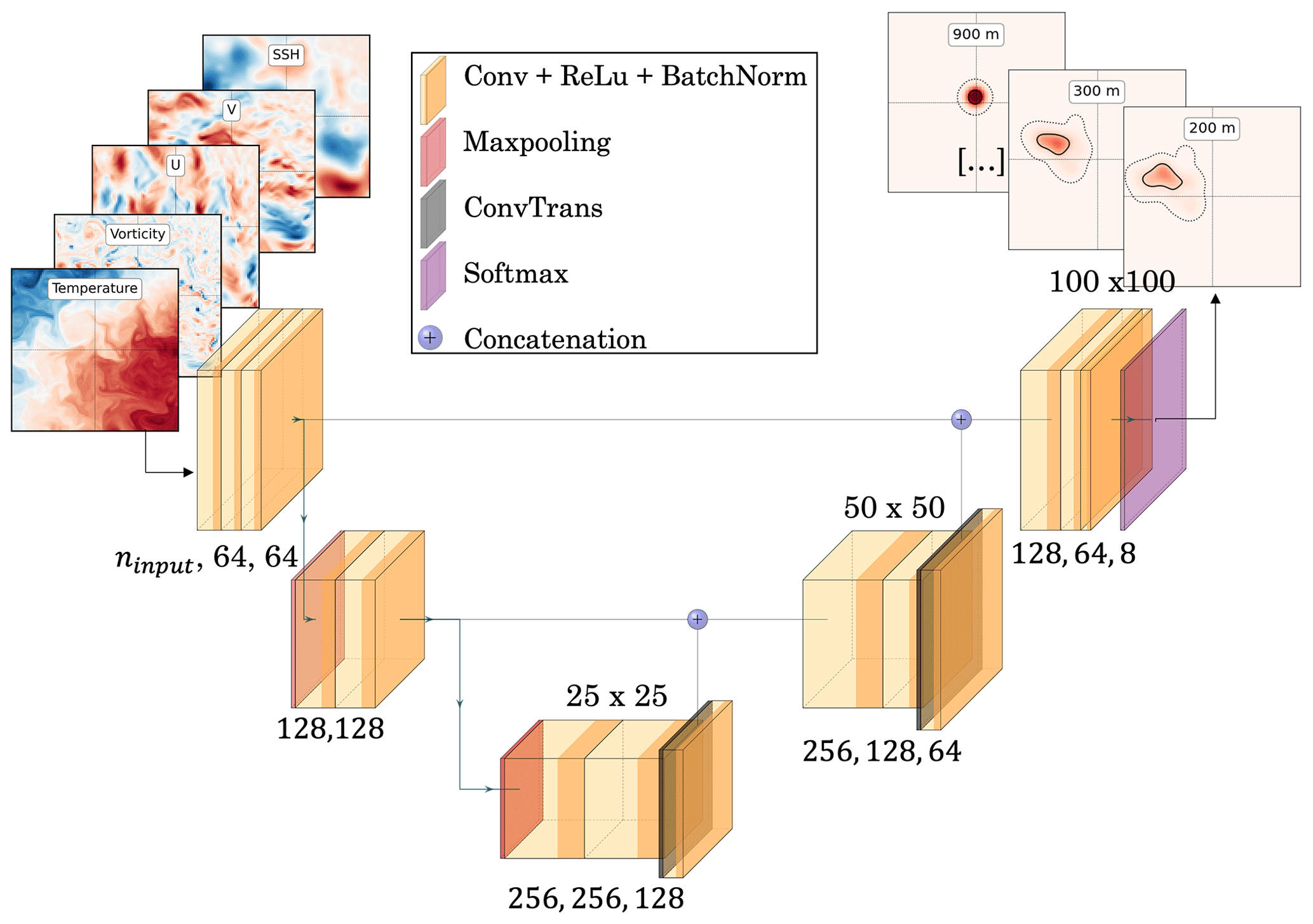
Figure 4 General U-Net architecture. The inputs include temperature, vorticity, u, v, and SSH images at multiple time steps and depths, concatenated with the initial PDFs (not shown). The outputs include the PDFs at eight depths, representing the distribution of the particles for each depth. At the top of each layer, the resolution of the images is shown, and at the bottom of each layer, the number of channels is shown.

3.3 Training scheme

We consider the Bhattacharyya coefficient (Bhattacharyya, 1943) as a training criterion to assess how well the predicted PDFs match the real ones. It is expressed as

$$\begin{array}{}\text{(1)}& {\mathrm{BC}}_z={\mathrm{\Sigma }}^{i\in D}\sqrt{P_{i,z}{Q}_{i,z}},\end{array}$$

where D represents the PAP domain, P_i is the predicted probability, and Q_i is the true probability at point i and depth z. The Bhattacharyya coefficient provides a similarity score between two PDFs and is used to derive the Bhattacharyya training loss (BL),

$$\begin{array}{}\text{(2)}& {\mathrm{BL}}_z=\mathrm{1}-{\mathrm{BC}}_z.\end{array}$$

The value of BL_z ranges from 1 to 0, with 0 representing a perfect prediction. During the training phase, we aim to minimize the loss function (ℒ), expressed as

$$\begin{array}{}\text{(3)}& \mathcal{L}={\displaystyle \frac{{\mathrm{BL}}_{\mathrm{200}\mathrm{m}}+{\mathrm{BL}}_{\mathrm{300}\mathrm{m}}+\mathrm{\dots }+{\mathrm{BL}}_{\mathrm{800}\mathrm{m}}+{\mathrm{BL}}_{\mathrm{900}m}}{n_{\mathrm{layer}}}},\end{array}$$

where ℒ is the mean of the BL computed at each of the eight vertical layers. The aim is to force the model to consider the evolution of particles along the water column. Empirically, this method improves the performance of the trained model in comparison to experiments where training loss is based only on BL_200 m.

We implement our deep learning scheme using PyTorch (Paszke et al., 2019). For the training phase, the Adam optimization algorithm (Kingma and Ba, 2015) is used with the following hyperparameters: β= (0.5, 0.999), zero weight decay, and a learning rate of 0.001. The training process is performed using mini-batches with a size of 32. After 50 training epochs, the best model is selected based on its performance using the evaluation data. We further improve the performance and robustness of the model using a bootstrapping method with 10 replicates (Breiman, 1996). The final prediction consists of a set of PDFs computed as the median of the predictions from the 10 models, followed by a re-normalization step. We also compute the standard deviation of the 10 predictions as a confidence index (see Sect. 5).

4 Results

We present the results of the numerical experiments conducted in the PAP case study. First, we detail a benchmarking experiment to evaluate the performance of the proposed deep learning schemes. Second, we further analyze how hydrodynamic conditions affect prediction performance.

Table 1 Scores and performance capabilities for different model architectures. For each model, we indicate the number of parameters, the average prediction score (BL_200 m), and the percentages of valid, quasi-valid, and non-valid test cases.

4.1 Prediction performance and comparison

We evaluate the performance of several models using the test database by employing the BL_200 m metric (i.e., the Bhattacharyya distance between the predicted PDF and the true PDF for the catchment area at 200 m of depth). We observe an empirical polynomial relationship between the BL score and the percentage of PDFs predicted, defined as ${\mathrm{\Sigma }}^{i\in D}min\left(P_{i,\mathrm{200}\mathrm{m}}{Q}_{i,\mathrm{200}\mathrm{m}}\right)$ (Fig. B1). We set up the following arbitrary evaluation criterion: a prediction is considered valid if the BL score is less than 0.2 and invalid if the BL score is greater than 0.3. These two thresholds correspond to percentages of predicted PDFs greater than or equal to 55 % and 45 %, respectively. For predictions with a BL score between 0.2 and 0.3, the global area is often still well predicted, but the values of the PDF are usually rough. In these cases, we create a third class called “quasi-valid”. Predictions in this class are not considered valid, but they still provide valuable information in the search for particle origins, and this information needs to be highlighted in the final score statistics.

We benchmark different models in Table 1. The U-Net_4 layers model is the U-Net architecture presented in Sect. 3, trained and tested with the D_4 layers database, which contains both surface and subsurface information. The U-Net_surf model only uses surface information from the D_surf database. The U-Net_surf-nb model is similar to the U-Net_surf model but does not use the bootstrap method. The CNN_surf-basic model includes a simple convolutional-neural-network (CNN) architecture consisting of a series of convolutional layers with a ReLU activation function, which we tested with D_surf. We also include a baseline prediction, which corresponds to the average of all the true PDFs used in the training database. This mean PDF roughly corresponds to a 2D Gaussian distribution centered on the PAP station, as presented in Wang et al. (2022).

The baseline and CNN_surf-basic models have poor performance, with zero valid cases. This highlights the complexity of the prediction task and the need for non-trivial models. It is noteworthy that the U-Net architecture seems to be well suited for this problem. The U-Net_surf-nb model achieves a very good performance, with 58 % of cases being valid, increasing to 66 % with the use of bootstrapping. Taking the quasi-valid predictions into account, ∼ 85 % of the predictions provide valuable information with only surface data. However, a comparison between the U-Net_4 layers and U-Net_surf models demonstrates the importance of subsurface information for obtaining more accurate and robust predictions. With 81 % of cases being valid and 13 % of cases being quasi-valid, the U-Net_4 layers model clearly outperforms the U-Net_surf model. This means that in about 10 %–15 % of cases, subsurface data are required to make valid predictions. Figure 5 shows examples of predictions from the test database using the U-Net_4 layers and U-Net_surface models. The PDFs are represented by two types of contour: one containing 99 % of the particles (dotted contours) and the other containing 50 % of the particles (solid contours). Both models are effective in predicting the overall catchment area. However, valid predictions are mainly characterized by a well-predicted center of the PDF, which is usually more accurate for the U-Net_4 layers model. In the following, we only focus on predictions from the U-Net_4 layers and U-Net_surface models.

Table 2 Variables associated with the Lagrangian experiments. BL${}_{\mathrm{200}\mathrm{m}}^{\mathrm{surf}}$ and BL${}_{\mathrm{200}\mathrm{m}}^{\mathrm{4}\mathrm{L}}$ indicate the Bhattacharyya loss at 200 m for the surface and four-layer models. We computed the mass centers (in kilometers) and entropy of the PDFs. MKE and EKE (cm² s⁻²) are computed with a temporal window of 30 d (the period of the Lagrangian experiment) and averaged between 200 and 1000 m in a 400 km box centered on the ST. Moreover, $\mathit{\zeta }/f$ and $\mathrm{OW}/f$ are computed from a surface snapshot taken 20 d after the first particle release and averaged within a 100 km box centered on the ST. The values of the median, 10th percentile, and 90th percentile are given at the top. Index numbers correspond to the examples given in Fig. 5.

Figure 5 Examples of predictions. PDFs are predicted with the U-Net_4 layers model (red) and the U-Net_surf model (green). Black contours represent the true origins of the particles. Dotted contours encompass 99 % of the particles, while solid contours encompass 50 %. The BL_200 m scores for both predictions are provided in the top-right corner of each plot. The background of each plot shows a snapshot of SSH taken 20 d after the first particle release, with surface velocities represented by the arrows. All the images are centered on the trap where particles are released.

4.2 Statistical analysis of the performance

We quantitatively analyze the potential causes of valid or invalid predictions. The examples show that the shape of particle distributions has a significant impact on score prediction. We find that PDFs located far from the STs, with mass centers > 150 km (i.e., the average distance between particles and their source), are generally not well predicted (Fig. 5; indices 16, 21, and 25 in Table 2). Similarly, complex PDF shapes characterized by multiple patches spread across the domain (see indices 2, 15, and 16 in Fig. 5) appear difficult to predict. Entropy (−Σp_ilog (p_i), where p_i is the PDF value at point i) characterizes the complexity of the PDF beyond its variance. Entropy increases with the spread of particles and in multimodal distributions, and high entropy values (> 6.6) could explain the prediction bias in some cases (indices 2, 15, and 16 in Table 1). This trend is confirmed by a statistical analysis over the entire test dataset, shown in Fig. 6. For PDFs with a mass center greater than 200 km, the probability of obtaining a valid prediction with the U-Net_surf model is less than 30 %. Similarly, we observe a trend of progressive degradation in the scores for PDFs with an entropy value higher than 6.6 (Fig. 6b).

Several physical factors could be responsible for the final PDF shape. To characterize the local dynamics, we compute the mean kinetic energy (MKE) and the eddy kinetic energy (EKE) around the ST as follows:

$$\begin{array}{}\text{(4)}& \underset{\mathrm{KE}}{\underbrace{{\displaystyle \frac{\mathrm{1}}{\mathrm{2}}}\left(\stackrel{\mathrm{‾}}{u^{\mathrm{2}}+v^{\mathrm{2}}}\right)}}=\underset{\mathrm{MKE}}{\underbrace{{\displaystyle \frac{\mathrm{1}}{\mathrm{2}}}({\stackrel{\mathrm{‾}}{u}}^{\mathrm{2}}+{\stackrel{\mathrm{‾}}{v}}^{\mathrm{2}})}}+\underset{\mathrm{EKE}}{\underbrace{{\displaystyle \frac{\mathrm{1}}{\mathrm{2}}}\left(\stackrel{\mathrm{‾}}{{u^{\prime }}^{\mathrm{2}}+{v^{\prime }}^{\mathrm{2}}}\right)}},\end{array}$$

where u and v are the two components of the horizontal ocean velocity. Here, $\stackrel{\mathrm{‾}}{u}$ and $\stackrel{\mathrm{‾}}{v}$ are the velocities averaged over a 30 d window, corresponding to the characteristic time period of our Lagrangian experiments. Finally, u^′ and v^′ are defined as follows:

$$\begin{array}{}\text{(5)}& {\displaystyle }{u}^{\prime }=u-\stackrel{\mathrm{‾}}{u},\text{(6)}& {\displaystyle }{v}^{\prime }=v-\stackrel{\mathrm{‾}}{v}.\end{array}$$

MKE and EKE are spatially averaged within a 400 km box around the ST and vertically averaged between 200 and 1000 m. These averages are computed every 10 d. MKE can be associated with large-scale currents and mesoscale eddies that stay stable during the time window. High MKE implies strong velocities that are likely to transport particles far from their source, further complicating the prediction process. EKE typically indicates the presence of moving mesoscale eddies or submesoscale fronts. These smaller-scale dynamics can promote divergent flows and increase entropy, thereby affecting the prediction score.

The number of invalid predictions increases on average with both MKE and EKE (Fig. 6c and d), even though the relationship between the prediction and EKE/MKE is not always simple when considering all cases listed in Table 2. Moreover, the influence of MKE seems to explain the seasonal patterns observed during the 5-year period of temporal coverage (Fig. 7). For both U-Net models, the best performance was achieved in winter/early spring, while the highest probability of non-valid predictions was observed in summer. We found a strong correlation (r²=0.64) between this trend and the seasonal evolution of MKE. This observation suggests that MKE could be the main driver of the score across long timescales. The EKE evolution shows a weaker correlation (r²=0.13). In particular, the EKE peak visible in April, associated with the deepest mixed layer and intensified submesoscale activity down to 500 m (Buckingham et al., 2016), is not clearly reflected in the performance score.

Figure 6 Fraction of non-valid predictions (BL_200 m>0.2) with respect to the following local dynamical variables: (a) PDF mass center shift, (b) PDF Shannon entropy (−Σplog(p)), (c) eddy kinetic energy (EKE), (d) mean kinetic energy (MKE), (e) relative surface vorticity ($\mathit{\zeta }/f$), (f) the surface relative Okubo–Weiss parameter (OW/f²), (g) the sea-level anomaly (SLA), and (h) the standard deviation (SD) of the 10 bootstrap models. In panels (c) and (d), energy is averaged within a 400 km box centered on the ST and between 200 and 1000 m. A temporal averaging window of 30 d is used for MKE and EKE. In panels (e), (f), and (g), the local dynamical variables come from surface snapshots taken 20 d after the first particle release and are averaged within a 100 km box around the ST.

Figure 7 Monthly performance statistics over the testing period for the U-Net_surf and U-Net_4 layer models. The bar graph indicates the probability of non-valid predictions (BL_200 m>0.2). The monthly averaged evolution of EKE (dotted) and MKE (dashed) between 200 and 1000 m is shown in black.

However, Table 2 suggests that MKE and EKE alone cannot explain the prediction score in all cases. The presence of coherent vorticity structures above the trap appears to facilitate prediction (indices 4, 11, and 17 in Fig. 5). To demonstrate this, we analyze dynamical features using three indicators: surface relative vorticity ($\mathit{\zeta }=v_x-u_y$), the Okubo–Weiss parameter (OW = σ²−ζ², where $\mathit{\sigma }=(u_x-v_y)+(v_x+u_y)$), and the sea-level anomaly ($\mathrm{SLA}=\mathrm{SSH}-<\mathrm{SSH}>$, where $<\mathrm{SSH}>$ is the average SSH within the subdomain). In order to avoid any smoothing effect, these variables are taken from a surface snapshot taken 20 d before the first particle release (rather than from an average over the experiment period). The particles reach a depth of approximately 200 m between days −15 and −25 following the initial release. Consequently, the 20th day represents the oceanic conditions present when the majority of particles are near the surface and under the influence of surface currents. The variables are averaged within a 100 km × 100 km area centered on the ST (Fig. 6e, f, and g; Table 2). The best performances (> 80 % of valid predictions) are associated with low negative OW values, high absolute ζ values, and significant SLA values. This situation generally corresponds to the presence of a vortex structure above the trap (Wang et al., 2022). On the other hand, chaotic situations characterized by OW values greater than 0, ζ values of ∼ 0, and SLA values of ∼ 0 are generally associated with the worst performance.

The presence of large-scale currents and eddies appears to be sufficient for explaining the prediction scores to a first-order approximation: high kinetic energy (KE) is typically associated with lower scores, unless coherent structures are present above the trap (corresponding to high KE with negative OW values and large vorticity amplitudes). This is highlighted by the bin statistics in Fig. 8. The non-valid prediction area in Fig. 8a is defined by KE>160 cm² s⁻² and $\mid \mathit{\zeta }/f\mid$ <0.05 and is characterized by an average Bhattacharyya score greater than 0.2 (indicated by the red bins). This chaotic situation represents 27 % of our dataset. Similarly, the same non-valid prediction zone can be observed in Fig. 8b and is defined by KE>160 cm² s⁻² and $\mathrm{OW}/f>-\mathrm{0.0075}$.

Figure 8 Averaged bin statistics of the U-Net_surf prediction score with regard to (a) kinetic energy vs. relative vorticity and (b) kinetic energy vs. the surface relative Okubo–Weiss parameter. Color represents the mean Bhattacharyya score. Bins with fewer than five samples are masked. The dashed black lines delineate the non-valid prediction zone, represented by the red bins.

5 Discussion

In this section, we discuss possible interpretations of the results, present the limitations of the model, and explore potential improvements that will guide our future work.

5.1 Interpretation of the statistics and confidence index

Our results support the relevance of the proposed machine learning approach in predicting the catchment area of particles using only surface data. Although subsurface information can improve the quality of the prediction, it is not essential in most cases. Analysis of the drivers of the prediction scores reveals complex, multifactorial causes. Only a few indicators were chosen for this analysis, and we do not exclude the possibility of other links that have not been investigated. However, the statistics appear coherent to us as they suggest that the model is more robust under weak and/or stable dynamics. Given that our model is limited in time and space by the 8 km input resolution (limited to the surface or four vertical layers, with snapshots taken every 10 d), it is clear that the predictions are sensitive to finer spatial and temporal variability. This may explain the good performance with low KE or in the presence of coherent eddies above the trap. Eddy structures can have a clear surface signature that is easy to identify and that stays coherent at depth (Fig. 2). Considering a 30 d period, these structures are generally stable, showing little temporal variability and limiting the spatial dispersion of particles trapped inside. In contrast, chaotic situations, typically characterized by randomly distributed submesoscale fronts with a horizontal size of about 10 km, are more likely to be less well predicted. Additionally, such structures can be too small to be detected. Temporal evolution can be very fast (on the order of days) and is unlikely to be adequately captured by our machine learning models. In the future, such assumptions may directly aid in developing a confidence index that depends on local dynamics. For future real-world applications, it will probably be difficult to predict the catchment area in every situation. The aim is, therefore, to understand in which situations the predictions made by the machine learning model can be trusted. In this respect, the standard deviation (SD) of the 10 model predictions from the bootstrap method (Fig. 6h) can also provide insight into quantifying the uncertainties in the predictions. The SD, computed as the mean SD of the 10 models at each prediction point, shows a linear relationship with the probability of having a valid prediction for the U-Net models. Previous studies have also explored such bootstrapping methods for uncertainty quantification (Pauthenet et al., 2022; Beauchamp et al., 2022; Haynes et al., 2023). Future work could also explore more advanced deep learning schemes with built-in uncertainty quantification properties (Haynes et al., 2023). However, it is worth noting that it would also be important to evaluate other sources of uncertainty, such as sinking-velocity distributions, simplifications of numerical simulations, and transport rates.

5.2 Towards real data and a more realistic representation of particles

The results strongly suggest the potential for using satellite data (SSH and sea surface temperature (SST)) to more precisely identify the source areas of particles collected in the deep ocean. A possible strategy for validating the model predictions against real observations would involve evaluating the cross-correlation between satellite chlorophyll in the prediction area and carbon fluxes measured at the PAP station (Frigstad et al., 2015). The cross-correlation coefficient can be compared with the obtained cross-correlation by considering a simplified catchment area, such as a 100 or 200 km box around the PAP location, which is a classical method still used today (Lampitt et al., 2023). If a better correlation is found, this indicates a better connection between deep fluxes at the PAP station and surface images from satellites and confirms the relevance of the model's application to real observations. As emphasized by Febvre et al. (2024) with respect to the learning-based mapping of sea surface dynamics, the representativeness of numerical simulations in reflecting real (3D + T) hydrodynamic conditions is likely to be a critical feature when applying a neural model trained on simulation data to a real-world configuration. The use of ocean reanalyses (Frigstad et al., 2015) could also be a relevant solution. In both cases, an in-depth analysis of 3D ocean circulation seems particularly important to assess the potential limitations of the proposed scheme.

Regarding biology, we consider STs at 1000 m, whereas in reality, the STs at the PAP station are moored at a greater depth (∼ 3000 m). It has been shown that below 1000 m, currents are weaker and do not significantly affect the horizontal displacement of particles (Wang et al., 2022). Therefore, although the influence of ST depth on prediction scores needs to be investigated, it can be assumed that it will not significantly affect model performance. However, a major bias in the model probably comes from the representation of carbon particles. We represent sinking particles with a settling velocity of 50 m d⁻¹, whereas, in reality, particles exhibit a wide range of velocities that can vary significantly with the seasons (Villa-Alfageme et al., 2016). The origins of particles can be very different depending on their sinking velocity, meaning it is important to consider the entire particle velocity spectrum to represent the catchment areas for particles with different velocities (Wekerle et al., 2018). Therefore, the next step of this study will focus on the effect of sinking velocities on prediction scores. We can assume that predicting catchment areas for particles with higher speeds than 50 m d⁻¹ may be more efficient as the particle trajectories are less impacted by currents and turbulence (Liu et al., 2018; Wekerle et al., 2018; Ma et al., 2021; Wang et al., 2022). However, particles with lower sinking velocities are more sensitive to the flow and can easily be dispersed over a large area far away from the ST, decreasing the prediction score, as suggested in Fig. 6a and b.

The use of a coupled biogeochemical model embedded in POLGYR could provide information on surface chlorophyll distribution (i.e., sea color) and primary-production (PP) intensity (Kostadinov et al., 2009; Dunne et al., 2005). Although these relationships are not direct (Laurenceau‐Cornec et al., 2020; Iversen and Lampitt, 2020; Cael et al., 2021), high PP levels are associated with large phytoplankton cells and particles, which may be associated with higher sinking rates. It is then possible to weigh the distribution of particles in terms of size and sinking velocity against the PP estimated by the model at their export locations, which should make the simulations more realistic. In addition, sea color observations, together with altimetry data, can be used as input for a machine learning system to better constrain carbon fluxes at depth, employing an approach similar to that presented here. However, the size and sinking velocity of particles are affected by numerous biological processes during their journey, which are generally not taken into account in simple Lagrangian studies. Although a Lagrangian approach could be developed (Jokulsdottir and Archer, 2016), an ad hoc parameterization, e.g., a parameterization derived from biogeochemical (BGC) models simulating particle dynamics (Aumont et al., 2015), could also be used and tested.

6 Conclusions

Identifying the origin of particles captured by sediment traps is important for interpreting measured fluxes and improving sampling methods. However, it remains complex to constrain particle motion at depth with surface data. In our study, we use the proposed machine learning scheme to address this issue. We demonstrate the ability of machine learning to predict, in real time, the origin of particles trapped in a PAP sediment trap at 1000 m of depth using realistic 3D numerical simulations and Lagrangian tracking. The evaluation of the machine learning models supports the use of a sea-surface-only configuration for the relevant prediction of particle catchment areas in most cases, suggesting a potential application with satellite data. The statistical analysis also shows that the prediction performance is sensitive to local dynamics. The model performs better under conditions of low KE and in the presence of coherent surface vortices above the sediment trap. The next challenges are to improve the particle modeling by considering the wide range of particle sinking velocities and to apply our model to real satellite data. Ultimately, this will improve the link between observations of surface and deep-carbon transport.

Appendix A: Comparison between POLGYR1 and POLGYR2

Figure A1 Snapshots of surface relative vorticity taken on 24 July 2003 (00:00 UTC) for POLGYR1 (a) and POLGYR2 (b). Despite the fact that similar forcing is applied to the two simulations, the surface dynamics are different due to distinct initial conditions and chaotic effects.

Appendix B: Relationship between the BL score and the percentage of PDFs predicted

Figure B1 Scatterplot of the average U-Net_surf Bhattacharyya score (BL_200 m) vs. the percentage of particles that are predicted, defined as ${\mathrm{\Sigma }}^{i\in D}min\left(P_{i,\mathrm{200}\mathrm{m}}{Q}_{i,\mathrm{200}\mathrm{m}}\right)$. The 4D polynomial relationship is shown with a black line. The vertical dashed lines represent the limits of the valid, quasi-valid, and non-valid zones.