Factors influencing the meridional width of the equatorial deep jets

Equatorial deep jets (EDJs) are vertically alternating, stacked zonal currents that flow along the Equator in all three ocean basins at intermediate depth. Their structure can be described quite well by the sum of high-baroclinic-mode equatorial Kelvin and Rossby waves. However, the EDJ meridional width is larger by a factor of 1.5 than inviscid theory predicts for such waves. Here, we use a set of idealised model configurations representing the Atlantic Ocean to investigate the contributions of different processes to the enhanced EDJ width. Corroborated by the analysis of shipboard velocity sections, we show that widening of the EDJs by momentum loss due to irreversible mixing or other processes contributes more to their enhanced time mean width than averaging over meandering of the jets. Most of the widening due to meandering can be attributed to the strength of intraseasonal variability in the jets' depth range, suggesting that the jets are meridionally advected by intraseasonal waves. A slightly weaker connection to intraseasonal variability is found for the EDJ widening by momentum loss. These results enhance our understanding of the dynamics of the EDJs and, more generally, of equatorial waves in the deep ocean.

1 Introduction

Equatorial deep jets (EDJs) are strong zonal currents in the deep equatorial oceans. They take the form of vertically stacked jets that alternately flow eastwards and westwards along the Equator, with a vertical scale of a few hundred metres (Luyten and Swallow, 1976; Hayes and Milburn, 1980; Leetmaa and Spain, 1981; Eriksen, 1982; Youngs and Johnson, 2015). In the Atlantic, they are not steady in time but show downward phase propagation on an interannual timescale. The EDJs are important for oceanic tracer transport at intermediate depth, e.g. contributing to the ventilation of the eastern tropical oxygen minimum zones (Brandt et al., 2012, 2015), and the deficiency of current ocean and climate models in simulating the jets contributes to the difficulties that the models have with simulating the observed biogeochemical tracer distributions (Getzlaff and Dietze, 2013; Dietze and Loeptien, 2013). Additionally, the EDJs probably influence climate variables in the surface ocean and lower atmosphere. Brandt et al. (2011) have found variability at the frequency of the Atlantic equatorial deep jets in observed surface currents, sea surface temperature, surface winds, and rainfall, while Matthießen et al. (2015) showed an impact of EDJs on the surface flow of the North Equatorial Countercurrent in idealised model simulations. However, despite the EDJs' importance for the equatorial ocean and surface climate, there are several gaps in our understanding of their generation mechanisms and their dynamics.

Although the EDJ generation mechanisms are still not entirely clear, it is thought that they are excited by intraseasonal Yanai waves that originate from instabilities in the western boundary currents and/or between the near-surface ocean currents, for example in the form of tropical instability waves (d'Orgeville et al., 2007; Hua et al., 2008; Ascani et al., 2015; Ménesguen et al., 2019). Tropical instability waves are generated near the surface, but they sometimes excite intraseasonal variability that can propagate to depths of a few thousand metres (Tuchen et al., 2018; Körner et al., 2022), where they can provide energy to the EDJs. Similarly, sources of intraseasonal wave energy were identified within the Equator-crossing deep western boundary current in observations and model simulations (Körner et al., 2022). Apart from exciting the EDJs, the intraseasonal Yanai waves also continuously maintain them through a mechanism whereby the equatorial deep jets deform the Yanai waves, which leads to a non-zero net eddy momentum flux reinforcing the EDJs (Greatbatch et al., 2018; Bastin et al., 2020).

d'Orgeville et al. (2007), Ascani et al. (2015), and Matthießen et al. (2017) have shown that the Atlantic EDJs are dynamically very similar to a resonant equatorial basin mode consisting of equatorial Kelvin and Rossby waves, as described for an idealised inviscid case by Cane and Moore (1981). In these basin modes, the sum of an eastward-propagating equatorial Kelvin wave and its reflection as westward-propagating equatorial Rossby waves becomes resonant at a certain period, which corresponds to the time it takes the Kelvin and the gravest reflected Rossby waves to travel across the basin, and thus depends on the basin width and the baroclinic mode of the equatorial waves (Cane and Moore, 1981). The EDJs in the Atlantic correspond to a basin mode of approximately baroclinic mode 17, with a corresponding resonance period of 4.6 years (Claus et al., 2016; Bastin et al., 2022).

However, the structure of the EDJs shows some features that deviate from the theoretical appearance of such a sum of inviscid linear equatorial waves with the corresponding vertical scale. One of them is the jets' cross-equatorial width, which has been consistently observed to be larger by a factor of 1.5 than theoretically expected. Muench et al. (1994) found this enhanced meridional width for the EDJs in the Pacific Ocean from looking at a zonal velocity section between 3^∘ S and 3^∘ N as well as at 159^∘ W, averaged over 16 months. For the Atlantic EDJs, a widening by the same factor of 1.5 was shown by Johnson and Zhang (2003) from an analysis of shipboard CTD (conductivity, temperature, depth) profiles and was later confirmed by other studies, e.g. Youngs and Johnson (2015) and Bastin et al. (2022). What exactly causes this observed widening of the EDJs compared to theoretical expectations is still unclear, although there have been two different suggestions.

Muench et al. (1994) suggested that the widening was an artefact caused by time averaging over EDJs that meander due to meridional advection by intraseasonal waves. An alternative theory was put forward by Greatbatch et al. (2012). These authors suggested that lateral mixing of momentum along isopycnals could explain the enhanced width. This is because at the Equator, below the Equatorial Undercurrent, diapycnal mixing is known to be particularly weak (Dengler and Quadfasel, 2002; Gregg et al., 2003). Since the zonal flow of the EDJs is close to being in geostrophic balance, dissipation of momentum without a corresponding dissipation of the associated density anomalies must lead to a broadening of the jets, an idea that goes back to Yamagata and Philander (1985). While it turns out that the meridional flux of momentum in fact acts to maintain, and not dissipate, the jets (Greatbatch et al., 2018; Bastin et al., 2020), the basic idea put forward by Greatbatch et al. (2012) remains valid. Indeed, Yamagata and Philander (1985) demonstrated this mechanism in a shallow water model using Rayleigh friction and Newtonian damping to represent dissipation of momentum and diapycnal mixing, respectively. A broadening of the EDJs could therefore be explained by dissipation of the momentum of the EDJs in the presence of much weaker diapycnal mixing. Greatbatch et al. (2012) were able to demonstrate their mechanism using a shallow water model to simulate the EDJs. For the mechanism suggested by Greatbatch et al. (2012), any process by which the EDJs lose momentum could widen the jets. In fact, it was later shown that the EDJs lose momentum not only through dissipation, but also through nonlinear energy transfer to the time mean flow (Ascani et al., 2015; Bastin et al., 2020), which could also contribute to the enhanced EDJ width. In the following, we shall mostly refer to “dissipation of momentum” but with the understanding that this includes momentum loss by other means, e.g. transfer to the mean flow.

In this study, we want to address the open question of which of the suggested processes by Muench et al. (1994) and Greatbatch et al. (2012) are responsible for the cross-equatorial widening of the EDJs. We use different idealised model configurations of the tropical Atlantic Ocean to assess the relative importance of the two suggested mechanisms, i.e. the meandering through intraseasonal meridional advection versus the dissipation or loss of momentum, for the enhanced mean EDJ width. To validate our results, we also make use of shipboard velocity sections. Additionally, we investigate the relation between the strength of intraseasonal variability and the cross-equatorial width of the EDJs in the idealised model runs because both Muench et al. (1994) and Greatbatch et al. (2012) suggested that the widening of the EDJs about the Equator is connected to the intraseasonal variability in the deep equatorial ocean, although in the theory of Greatbatch et al. (2012) any processes which lead to enhanced dissipation or loss of momentum could also play a role.

Another open question which has not been addressed so far is the role of the amplitude ratio of the Kelvin wave and the first-meridional-mode Rossby wave in the EDJ basin mode for the enhanced EDJ width. The amplitude ratio could play a role in setting the width of the EDJs because the zonal velocity signature of an equatorial Kelvin wave has a larger cross-equatorial width than that of a first-meridional-mode long Rossby wave of the corresponding vertical mode. Youngs and Johnson (2015) have shown that the ratio of the Kelvin and Rossby wave amplitudes varies between the three ocean basins: in the Atlantic, the Rossby wave seems to dominate the EDJ signal, whereas in the Indian Ocean and Pacific Ocean, the contributions of the two waves are more similar. So far, the 1.5-fold widening of the EDJs has mostly been estimated in comparison to the expected width of an inviscid first-meridional-mode Rossby wave for the corresponding baroclinic mode, not the expected width of the entire inviscid basin mode (Muench et al., 1994; Johnson and Zhang, 2003; Youngs and Johnson, 2015). Therefore, the effect of the Kelvin and Rossby wave amplitude ratio for the meridional EDJ width is also investigated here.

The article is structured as follows: in Sect. 2, the model configurations and analysis methods are described. In Sect. 3, the results are presented, starting with an overview of the model configurations' ability to simulate EDJs and a description of the differences in the cross-equatorial width of the EDJs in Sect. 3.1. This is followed by Sect. 3.2 wherein the amplitude contributions of the equatorial Kelvin and first-meridional-mode Rossby wave to the EDJs are discussed. The importance of meandering of the EDJs versus widening by dissipation or momentum loss in setting their time mean cross-equatorial width is investigated in Sect. 3.3, as is the relationship between the meridional EDJ width and the intraseasonal variability in the models. Finally, a discussion of the results is provided in Sect. 4.

2 Model and methods

2.1 Model configurations

The ocean model that has been used for all simulations shown here is the Nucleus for European Modelling of the Ocean (NEMO, Madec et al., 2017) version 3.6. The basic model setup is based on the studies by Ascani et al. (2015) and Matthießen et al. (2015, 2017), who succeeded in simulating EDJs with an idealised model of the tropical Atlantic, although they used the Parallel Ocean Program (POP) and MITgcm ocean models instead of NEMO. All models are ocean-only simulations for a basin analogous to the tropical Atlantic, but with closed boundaries at 20^∘ S and 20^∘ N. The horizontal resolution is set to 0.25${}^{\circ }\times$ 0.25^∘. Following Ascani et al. (2015), the horizontal mixing of tracers and momentum is parameterised using biharmonic diffusion and viscosity with a coefficient of $-\mathrm{2}\times {\mathrm{10}}^{\mathrm{10}}$ m⁴ s⁻¹, and the vertical mixing scheme is Richardson-number-dependent (Pacanowski and Philander, 1981) with a background diffusivity of 10⁻⁵ m² s⁻¹. The TEOS-10 equation of state is used for all simulations. All model runs are initialised with a horizontally homogeneous density field derived by horizontally and temporally averaging vertical profiles of tropical Atlantic (between 20^∘ S and 20^∘ N) salinity and temperature from the World Ocean Atlas 2018 (WOA18, Locarnini et al., 2019; Zweng et al., 2019). The in situ temperature and practical salinity from WOA18 have been converted to conservative temperature and absolute salinity with a Python implementation of the Gibbs Sea Water Library (Firing et al., 2019). At the surface, the temperature and salinity are restored to their initialisation value with a damping timescale of 30 d to maintain a reasonable stratification of the water column over time.

The model setup from which all the others are derived is called L200-WIND. Its domain is rectangular with a width of 55^∘ to mimic the Atlantic Ocean at the Equator, and it has a flat bottom at 5000 m depth. There are 200 model levels, with a vertical resolution of 5 m close to the surface, approximately 20 m in the depth range of the EDJs, and increasing to 50 m close to the bottom. L200-WIND is forced with zonally and temporally averaged wind stress from the NCEP/NCAR reanalysis (Kalnay et al., 1996; Kistler et al., 2001). It has a free-slip boundary condition at the bottom because Ascani et al. (2015) found that bottom friction reduces the ability of the model to simulate EDJs. Although only zonally and temporally averaged wind forcing is applied, the upper-ocean zonal currents are relatively well reproduced and create enough shear for instabilities to develop and generate variability at depth. After a spin-up of about 50 years, realistic-looking EDJs develop in the wind-forced, flat-bottomed L200-WIND, as shown in Bastin et al. (2020) and also visible in Fig. 2 where Hovmöller diagrams of the zonal velocity in the centre of the model basin are shown for all model runs used here (continued in Fig. 3).

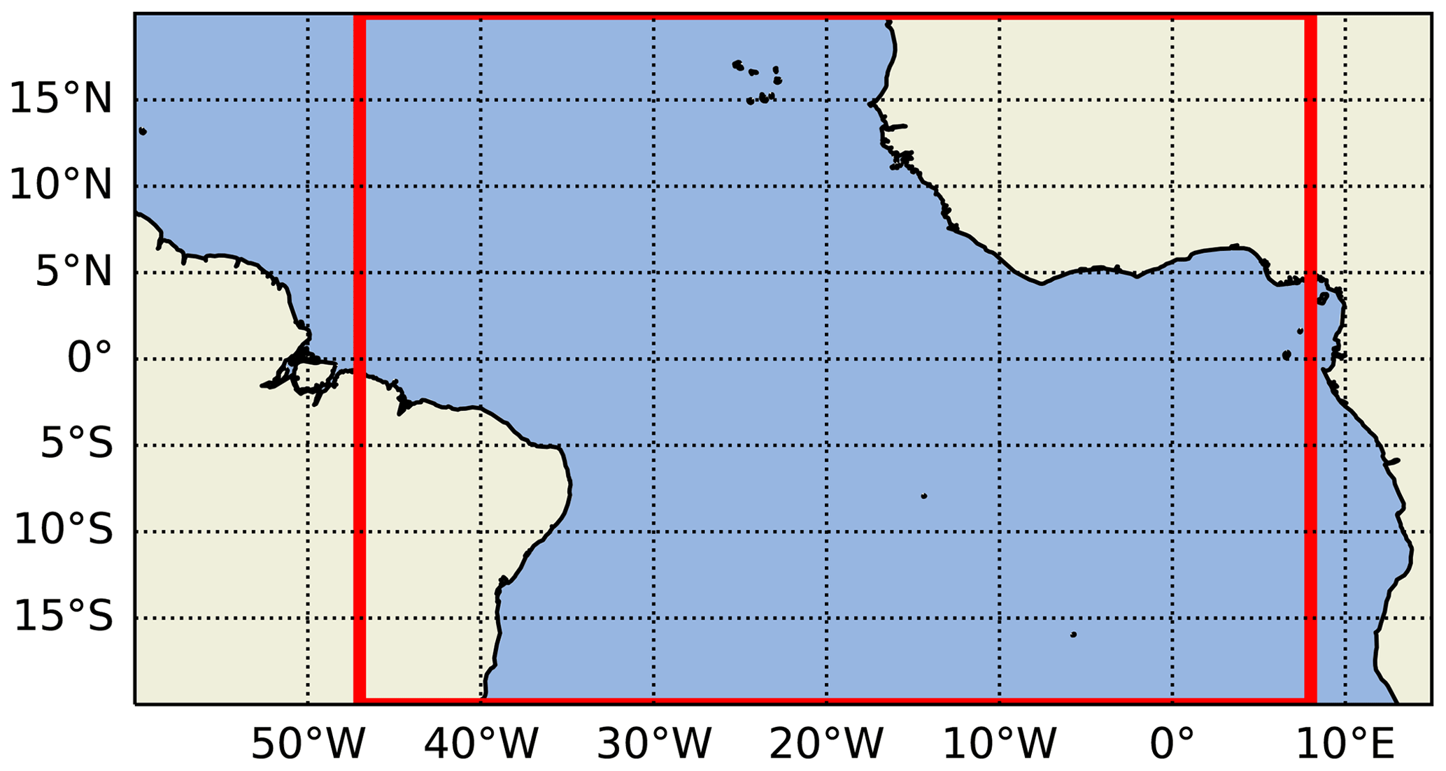
Figure 1 Model domain. The red line indicates the model domain for all configurations with a rectangular basin and a flat bottom at 5000 m depth. The entire figure shows the domain for all other configurations with a realistic tropical Atlantic coastline and bathymetry.

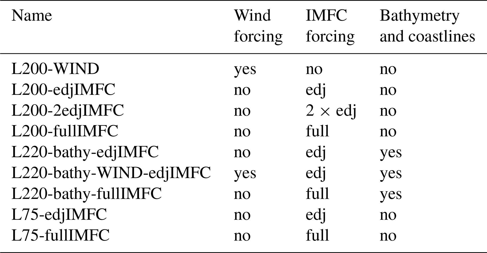
From the rectangular wind-driven configuration L200-WIND, a number of other model setups are derived, all of which are listed with their distinguishing features in Table 1. There are two different vertical resolutions marked by the number after the L in the configuration name. L200 is the fine vertical resolution, and L75 is a coarser one with 75 levels that is one of the commonly used vertical axes by NEMO ocean models, e.g. by the Global Seasonal forecast system of the MetOffice (MacLachlan et al., 2015). Note that there are some configurations that are named L220; these have the same vertical resolution as the rectangular, flat-bottomed L200 configurations but extend to depths greater than 5000 m and thus have additional layers at these depths because they include realistic bathymetry. Another difference between the configurations is the forcing. There are two types of forcing applied. First, the wind forcing, i.e. zonally and temporally averaged NCEP/NCAR wind stress, is either switched on or off. Second, there is the IMFC (intraseasonal momentum flux convergence) forcing, which is a tendency added to the zonal momentum equation in the model at every grid point and time step, as described in Bastin et al. (2020). It is the intraseasonal eddy flux convergence from the meridional advection term in the zonal momentum equation, i.e.

$$\begin{array}{}\text{(1)}& -{\displaystyle \frac{\partial \left(\stackrel{\mathrm{‾}}{u^{\prime }{v}^{\prime }}\right)}{\partial y}},\end{array}$$

where the prime denotes variability on timescales smaller than 70 d (or intraseasonal) and the overbar means variability on timescales larger than 70 d. This term is thought to be responsible for energy transfer from intraseasonal waves to the EDJs and other slowly varying currents (for details see Greatbatch et al., 2018). For the IMFC model forcing, the term (Eq. 1) is diagnosed from the base model configuration L200-WIND to be applied to other model configurations, as described in Bastin et al. (2020). There are two different flavours of IMFC forcing in the different model experiments: “edj” includes only one Fourier component of the IMFC, namely that with the frequency of the EDJs, and “full” includes the entire IMFC diagnosed from L200-WIND varying on all timescales. The “2edj” has the same forcing as “edj” but multiplied by a factor of 2. The last differences between the model setups concern the use of realistic coastlines and bathymetry. All model configurations that do not have realistic coastlines and bathymetry are rectangular and have a flat bottom like L200-WIND. The model setups that do have realistic coastlines and bathymetry have linear bottom friction instead of a free-slip bottom boundary condition like the flat-bottomed setups. Their northern and southern boundaries are still closed at 20^∘ S and 20^∘ N. In the cases in which the IMFC forcing diagnosed from the rectangular L200-WIND is applied to setups with realistic coastlines and bathymetry, it is only applied at points that exist in both configurations and set to zero otherwise. Because we chose the rectangular geometry to fit the width of the Atlantic basin at the Equator, this only happens away from the Equator and close to the coasts where it is not important for our analysis of the EDJs.

Some combinations of forcing and parameters that we tested did not support EDJs, e.g. bottom friction and/or realistic bathymetry without IMFC forcing as well as L75 without IMFC forcing. These are therefore not included here.

Table 1 Overview of model runs.

2.2 Analysis methods

2.2.1 Vertical normal mode decomposition

The EDJs, unlike most other large-scale flow patterns in the ocean, are characterised by relatively small vertical wavelengths. It is therefore instructive to separate the velocity field into its different vertical scales. This can be done by expressing the flow field's variation in the vertical as a sum of vertical normal modes to get a sum of linearly independent components of the velocity field, each of which has its unique vertical structure and varies only in the horizontal and time (for details see e.g. Kundu et al., 2012, Chapter 13.9.).

To obtain the vertical structure functions of the vertical modes, a mean buoyancy frequency profile from the model, averaged along the Equator, is used (in the case of the configurations with bathymetry only spanning the depth range where there is no bathymetry, i.e. extending to a depth of approximately 3500 m). The zonal velocity field from the model is then projected onto the vertical structure functions. The resulting u_n for each vertical mode n can then be analysed separately, e.g. by calculating vertical mode spectra as shown in Fig. 2. The separation into vertical normal modes is also used here to vertically filter the zonal velocity by summing only the u_n of modes 15 to 22 to remove variability different from the EDJs.

2.2.2 Quantification of meridional EDJ width

The cross-equatorial width of the EDJs has usually been given as the e-folding scale of the meridional profile of zonal velocity amplitude (e.g. Greatbatch et al., 2012). This is continued here. To ensure comparability across all the meridional width estimates given in this paper (e.g. also those of a theoretical inviscid Kelvin or Rossby wave), they are all determined by a fit of a Gaussian of the form

$$\begin{array}{}\text{(2)}& g\left(\mathit{\theta }\right)=a\cdot \exp \left(-{\displaystyle \frac{\mathrm{1}}{\mathrm{2}}}{\displaystyle \frac{(\mathit{\theta }-{\mathit{\theta }}_{\text{c}}{)}^{\mathrm{2}}}{{\mathit{\sigma }}^{\mathrm{2}}}}\right)\end{array}$$

to the zonal velocity between 1.5^∘ S and 1.5^∘ N. Here, a is the amplitude, θ denotes latitude, θ_c is the position of the EDJ core (or maximum), and the meridional width of the EDJs is given by $W=\sqrt{\mathrm{2}}\cdot \mathit{\sigma }$. The relatively narrow equatorial corridor between 1.5^∘ S and 1.5^∘ N is taken to reduce the influence of off-equatorial maxima in the zonal velocity field, such as associated with Rossby waves. The equatorial radius of deformation for a gravity wave speed of 16.2 cm s⁻¹ (corresponding to the EDJ peak baroclinic mode 19 from L200-WIND) is approximately 0.76^∘, well covered by the latitude range used for the fit. The width W of an inviscid first-meridional-mode Rossby wave of this particular vertical mode, determined by the Gaussian fit as described above, is 0.65^∘, and that of an inviscid Kelvin wave is 1.06^∘. The fitting of the EDJ width is done at all longitudes between 25 and 15^∘ W where the EDJs are strongest, and the width is then averaged over this longitude range.

The zonal velocity is filtered vertically before analysing the cross-equatorial EDJ width such that only the EDJ variability is included in the analysis. This is done by decomposing the zonal velocity into vertical normal modes (see previous section) and retaining only the contributions of the vertical modes 15 to 22, which cover the EDJ peak (shown in Figs. 2 and 3).

We determine both the long-time mean EDJ width, which should be comparable to that from other studies, and the EDJ width due only to (i) dissipation or momentum loss and (ii) averaging over meandering of the jets. The long-time mean EDJ width is determined by fitting Eq. (2) to the harmonic amplitude field of the vertically filtered zonal velocity varying at the EDJ period, which is approximately 4.4 years in the models, whereas the EDJ widening due to dissipation and the EDJ widening due to meandering are determined by fitting Eq. (2) to temporal snapshots of the vertically filtered zonal velocity field. The EDJ width due to dissipation is then given as $W=\sqrt{\mathrm{2}}\cdot \mathit{\sigma }$, which should not include any contribution from meandering since we allow the fitted profile to be displaced to the north or south and do the fit separately at every longitude and time. For the EDJ width due to meandering, the resulting distribution of the parameter θ_c, i.e. only the information about the shift of the EDJ core away from the Equator, is used to produce a distribution of theoretical first-meridional-mode Rossby wave zonal velocity amplitude profiles with corresponding meridional shifts. From these, an average profile is calculated and the e-folding scale of this is determined as described above. As a basis for comparison, we always use the width of an analytic inviscid first-meridional-mode Rossby wave to be consistent with previous studies: most studies that reported an increased meridional width of the EDJs used an inviscid first-meridional-mode Rossby wave of corresponding vertical scale and frequency as the theoretical comparison and on this basis calculated a widening of the EDJs by a factor of 1.5 (Johnson and Zhang, 2003; Youngs and Johnson, 2015).

2.2.3 Separation of Kelvin and first-meridional-mode Rossby waves

The contributions of the equatorial Kelvin wave and the first-meridional-mode Rossby wave to the EDJs are separated by a regression of the models' zonal velocity field onto the theoretical structures of the two waves, in which the meridional profile of zonal velocity of the respective wave is specified and the waves' frequency is fixed to the dominant EDJ frequency, which in the models is approximately f_EDJ = (4.4 yr)⁻¹. For both waves, a linear combination of a sine and a cosine with the respective frequency and meridional structure is fitted such that the problem takes the form of a linear regression with four degrees of freedom. The optimisation problem is given by the following term that is minimised using a Python implementation of a least squares linear regression (scipy.optimize.lsq_linear version 1.6.2).

$$\begin{array}{}\text{(3)}& \left|\right|{\mathbf{D}}_{i,j}\cdot {\mathit{b}}_j-{\mathit{u}}_i|{|}^{\mathrm{2}}\end{array}$$

Here, u is the zonal velocity, i a combined multi-index for time and latitude, b is the coefficient vector to be determined with index $j=(\mathrm{1},\mathrm{2},\mathrm{3},\mathrm{4})$, and the design matrix D is given by

$$\begin{array}{}\text{(4)}& \mathbf{D}={\left(\begin{array}{c}\cos (\mathit{\omega }\cdot t_i)\cdot u_{\text{K}}\left(y_i\right)\\ \sin (\mathit{\omega }\cdot t_i)\cdot u_{\text{K}}\left(y_i\right)\\ \cos (\mathit{\omega }\cdot t_i)\cdot u_{\text{R1}}\left(y_i\right)\\ \sin (\mathit{\omega }\cdot t_i)\cdot u_{\text{R1}}\left(y_i\right)\end{array}\right)}^T.\end{array}$$

The superscript T denotes the transpose of the matrix. The angular frequency ω=2πf_EDJ is set to that of the EDJs, t is the time, and y is the northward distance from the Equator in metres. The meridional profiles of the zonal velocity signatures of the Kelvin (u_K) and first-meridional-mode Rossby (u_R1) waves are given by the following equations (see Gill, 1982, Chapter 11)

$$\begin{array}{}\text{(5)}& {\displaystyle }{u}_{\text{K}}\left(y\right)=u_{\mathrm{0}\mathit{\_}\text{K}}\cdot \exp \left(-{\displaystyle \frac{\mathit{\beta }{y}^{\mathrm{2}}}{\mathrm{2}c}}\right),\text{(6)}& {\displaystyle }\begin{array}{rl}{\displaystyle }{u}_{\text{R1}}\left(y\right)& {\displaystyle }=u_{\mathrm{0}\mathrm{\_}\mathrm{R}\mathrm{1}}\cdot \exp \left(-{\displaystyle \frac{\mathit{\beta }{y}^{\mathrm{2}}}{\mathrm{2}c}}\right)\cdot \\ {\displaystyle }& {\displaystyle }[\left(c-{\displaystyle \frac{c}{\mathrm{3}}}\right)\cdot {\mathrm{2}}^{-\mathrm{1}}\cdot H_{\mathrm{2}}\left(\sqrt{{\displaystyle \frac{\mathit{\beta }}{c}}}y\right)-\left(c+{\displaystyle \frac{c}{\mathrm{3}}}\right)],\end{array}\end{array}$$

for long equatorial Rossby waves with meridional mode number 1. u_{0_K} and u_{0_R1} denote constant amplitude values which for the fit are chosen such that $u_{\text{K}}(y=\mathrm{0})=u_{\mathrm{R}\mathrm{1}}(y=\mathrm{0})=\mathrm{1}$ m s⁻¹, $\mathit{\beta }=\mathrm{2.3}\times {\mathrm{10}}^{-\mathrm{11}}$ m⁻¹ s⁻¹ is the change of the Coriolis parameter with latitude, and H₂ denotes the second Hermite polynomial. For the gravity wave speed we use a value of c=16.2 cm s⁻¹ corresponding to the EDJ peak baroclinic mode 19 from L200-WIND (the changes in the EDJ peak mode gravity wave speed are negligible between the model runs). u_K and u_R1 are stretched meridionally before the regression to account for the different meridional widths of the EDJs in the model configurations. The stretching factor is determined by detecting the mean latitude of the off-equatorial minima in the EDJ amplitude field and dividing this latitude by the latitude of the theoretical Rossby wave zonal velocity profile zero crossing.

The regression is done at all longitudes and depths. From the resulting coefficients b, the amplitude A and phase p of the Kelvin and Rossby wave can then be computed as follows.

$$\begin{array}{}\text{(7)}& {\displaystyle }{A}_{\text{K}}=\sqrt{\mathit{b}(\mathrm{1}{)}^{\mathrm{2}}+\mathit{b}(\mathrm{2}{)}^{\mathrm{2}}}\text{(8)}& {\displaystyle }{p}_{\text{K}}=\arctan \left(-{\displaystyle \frac{\mathit{b}\left(\mathrm{2}\right)}{\mathit{b}\left(\mathrm{1}\right)}}\right)\text{(9)}& {\displaystyle }{A}_{\text{R1}}=\sqrt{\mathit{b}(\mathrm{3}{)}^{\mathrm{2}}+\mathit{b}(\mathrm{4}{)}^{\mathrm{2}}}\text{(10)}& {\displaystyle }{p}_{\text{R1}}=\arctan \left(-{\displaystyle \frac{\mathit{b}\left(\mathrm{4}\right)}{\mathit{b}\left(\mathrm{3}\right)}}\right)\end{array}$$

3 Results

3.1 EDJs in the different model experiments

In Figs. 2 and 3, Hovmöller diagrams of the zonal velocity from the centre of the model basin are shown for all model configurations listed in Table 1. Spectra of the zonal velocity from the model basin centre are shown as well, calculated separately for the different vertical normal modes after mode decomposition. For the configurations with realistic coastlines, the centre of the basin here means halfway along the Equator between the coasts.

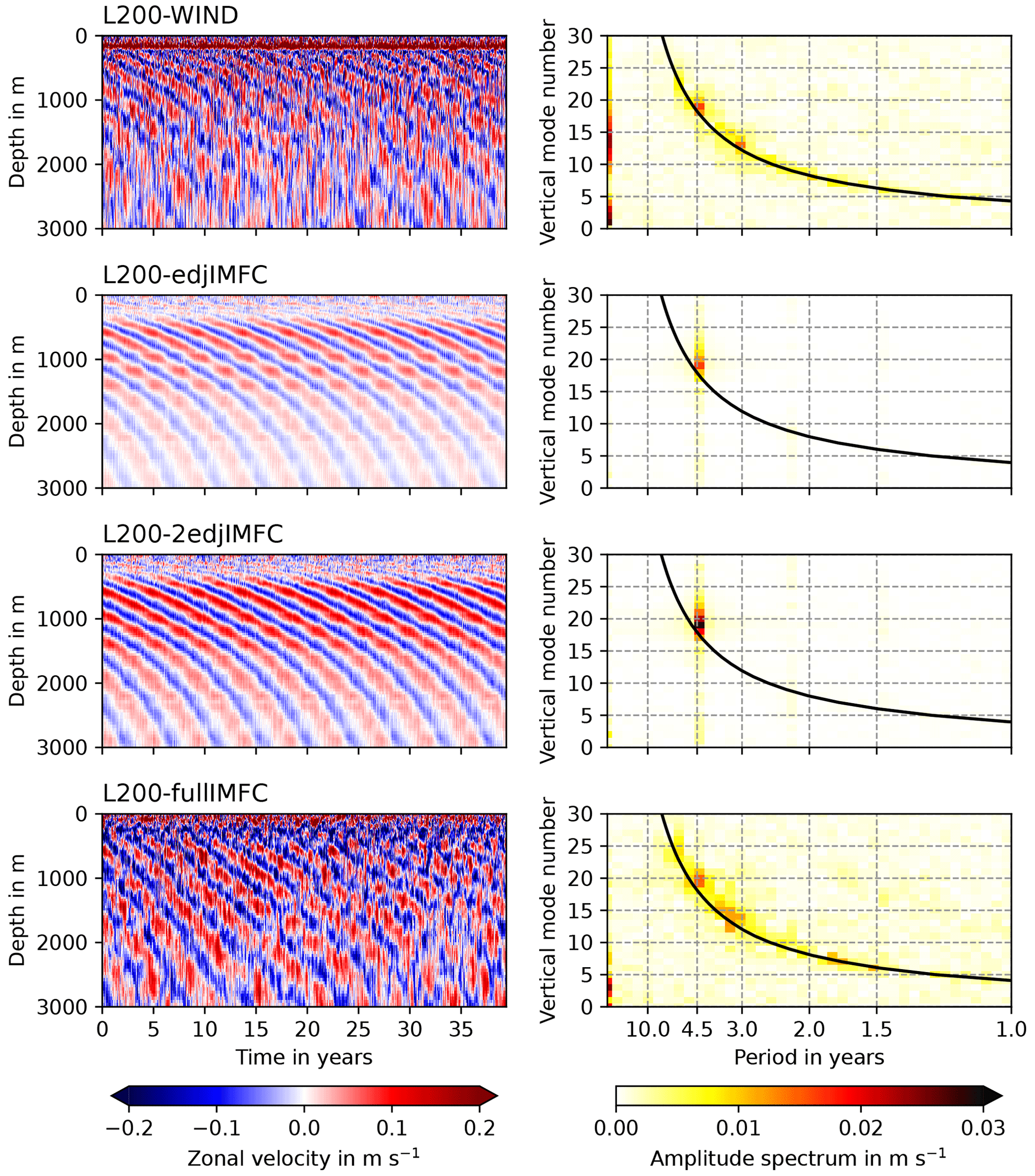
Figure 2 Hovmöller diagrams (left panels) and normal mode spectra (right panels) of the zonal velocity in the centre of the model basin for the model configurations L200-WIND, L200-edjIMFC, L200-2edjIMFC, and L200-fullIMFC. Positive zonal velocity values indicate eastward velocity, and negative values mean westward velocity. The solid black line in the right panels shows the resonance frequency for the gravest equatorial basin mode for each vertical normal mode. The spin-up is excluded from all model runs (50 years for wind-forced runs, 10 years for those without wind forcing). The normal mode structure functions are provided in the supplementary dataset; see the “Data availability” section (continued for other model runs in Fig. 3).

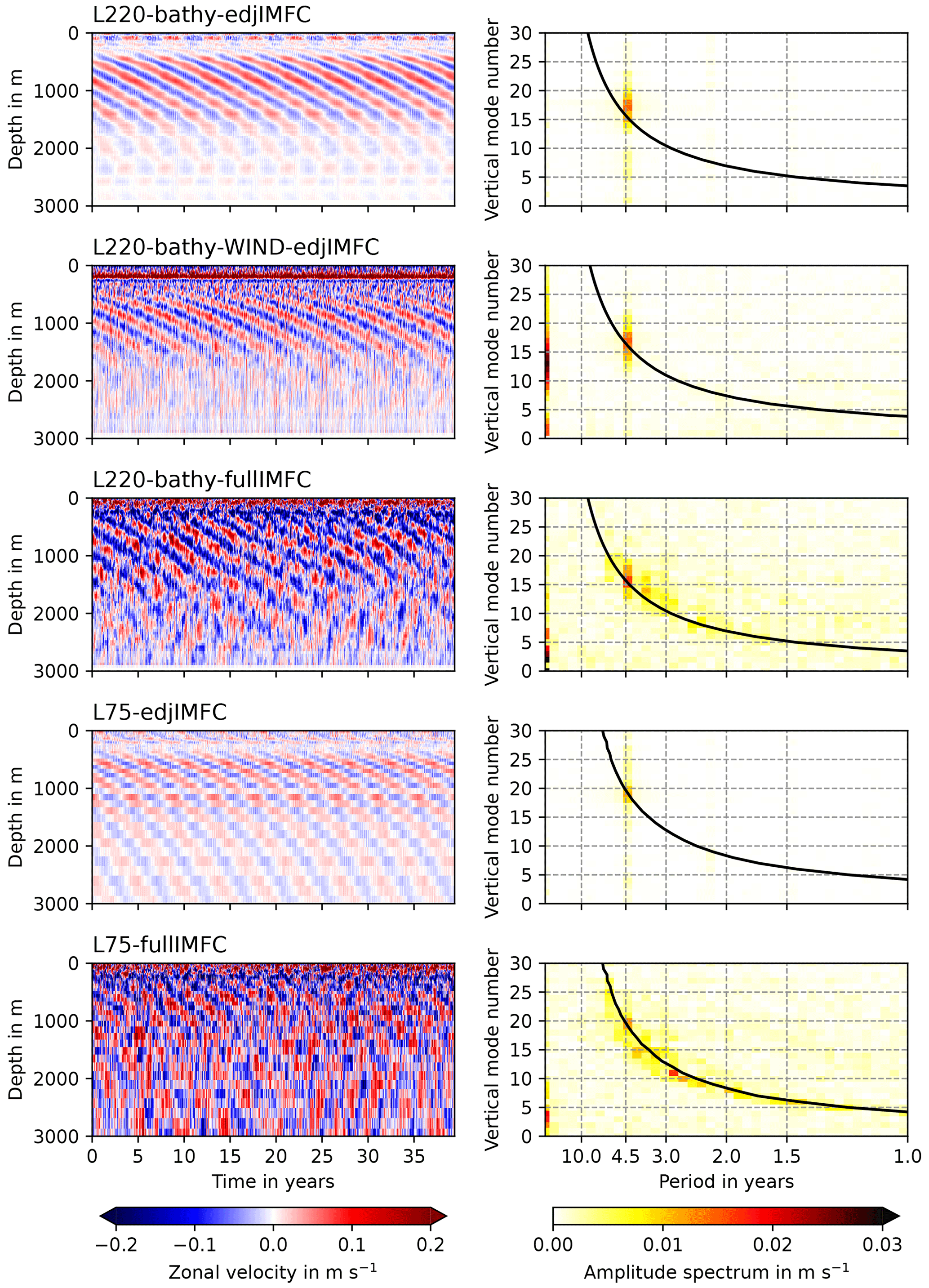
Figure 3 As Fig. 2, but for the model configurations L220-bathy-edjIMFC, L220-bathy-WIND-edjIMFC, L220-bathy-fullIMFC, L75-edjIMFC, and L75-fullIMFC.

The EDJs are visible in the Hovmöller diagrams of equatorial zonal velocity as vertically alternating, downward-propagating bands of currents. In the normal mode spectra, they appear as a peak close to the basin mode resonance curve at a period of about 4.4 years. The observed period of the real Atlantic EDJs is, at 4.6 years, slightly larger (Bastin et al., 2022).

The meridional structure of the EDJs becomes visible in snapshots of the zonal velocity field. Shown in Fig. 4 are 5 d means of the vertically filtered (modes 15 to 22 to show only the EDJ variability) zonal velocity at 1000 m depth, spaced 1 year apart, for two of the rectangular, flat-bottomed model runs: one driven by wind forcing (L200-WIND) and the other driven only by the EDJ frequency component of the intraseasonal momentum flux convergence (L200-edjIMFC). The EDJs are visible as strong zonal current bands on the Equator, changing direction every few years and propagating from the east towards the west. It is visible that the EDJs in L200-WIND have a larger meridional scale than those in L200-edjIMFC. Different mechanisms seem to contribute to the enhanced meridional EDJ width in L200-WIND: there is more meandering about the Equator of the EDJs that would lead to a larger meridional scale in the time mean EDJ signature compared to L200-edjIMFC as suggested by Muench et al. (1994), but the EDJs also seem to have a larger meridional width independent of meandering in L200-WIND than in L200-edjIMFC, which could indicate an irreversible widening through enhanced dissipation of momentum following Greatbatch et al. (2012). The influence of these two different factors on the time mean meridional width is investigated for all nine model configurations in Sect. 3.3.

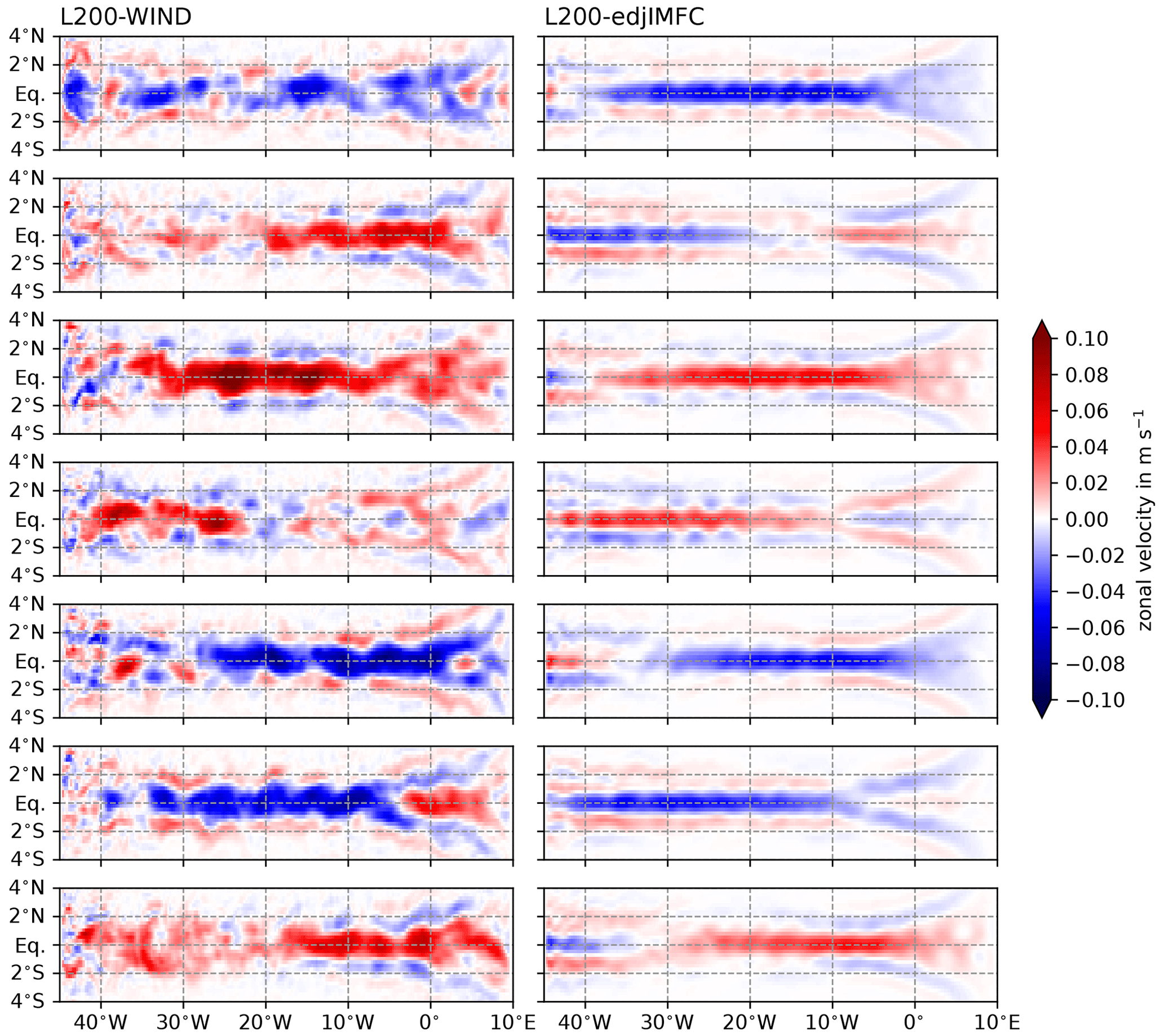
Figure 4 The 5 d means of zonal velocity at 1000 m depth in the L200-WIND and L200-edjIMFC model runs. The panels from top to bottom are each 1 year apart. The zonal velocity has been vertically filtered to contain only the baroclinic modes 15 to 22. Positive zonal velocity values indicate eastward velocity, and negative values mean westward velocity.

Across the nine model runs, the cross-equatorial width of the deep jets varies substantially. The mean meridional EDJ width for all of the nine model runs is shown in Fig. 5, together with the meridional width of an inviscid first-meridional-mode Rossby wave and an inviscid equatorial Kelvin wave with a corresponding vertical structure. The model runs are sorted by the mean meridional width of the EDJs, from small to large; this order will be kept for the following similar figures. In general, the mean meridional width of the EDJs is larger in model configurations with wind forcing or fullIMFC forcing. In contrast to that, models with only edjIMFC forcing, i.e. intraseasonal momentum flux convergence varying only at the interannual EDJ frequency, have the narrowest EDJs, although a doubling of the edjIMFC forcing leads to a slightly enhanced EDJ width (L200-2edjIMFC compared to L200-edjIMFC). Since variability on all other timescales is greatly reduced in the model runs forced only at the interannual EDJ frequency, the narrow EDJs in those models could be connected to a lack of variability, e.g. intraseasonal waves. This is investigated in Sect. 3.3, where the contributions of meandering and widening by dissipation to the time mean width of the EDJs are also separated. Also marked in Fig. 5 is the value of the Rossby wave width enhanced by a factor of 1.5. The exact value of the meridional Rossby wave scale is a bit arbitrary, since it depends on the choice of the vertical normal mode of the wave. In fact, the EDJs are composed of multiple normal modes rather than one distinct mode. Here the EDJ peak mode from L200-WIND is chosen (mode 19) for the theoretical inviscid wave widths just to give a visual impression of how much wider the observed EDJs are than the expected inviscid Rossby wave width (the grey dashed line compared to the black dashed line). The values for the Rossby wave width are a bit smaller here than usually obtained from observations of the Atlantic EDJs: Youngs and Johnson (2015), for example, estimated the Rossby wave width to be 0.73^∘, consistent with the lower vertical mode number 17 that they found for the Atlantic EDJ peak from observations.

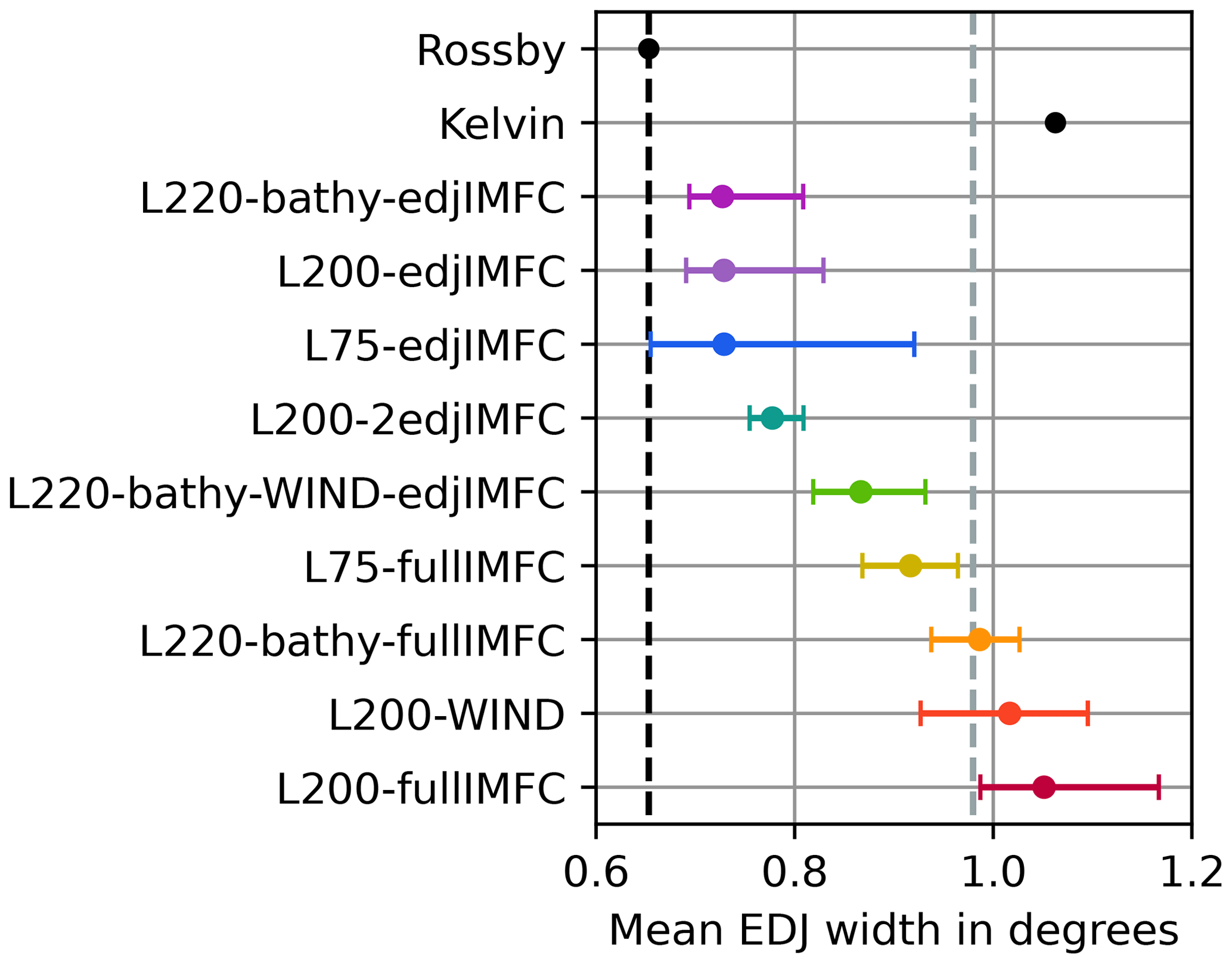
Figure 5 Mean cross-equatorial EDJ width in the different model experiments. For the nine model configurations that can simulate EDJs, the e-folding scale of a Gaussian fit to the time mean EDJ amplitude field between 25 and 15^∘ W is shown. The time mean EDJ amplitude field has been determined as the harmonic amplitude at the EDJ period (4.4 years) of the vertically filtered (modes 15 to 22) zonal velocity field from the models. The error bars mark the 68 % quantile of the mean EDJ width distribution across the different longitudes and depths (between 25^∘ W and 15^∘ W and between 400 and 2000 m depth). Also shown are the corresponding meridional widths of an inviscid first-meridional-mode Rossby wave (black dashed line), 1.5 times the width of the Rossby wave (grey dashed line), and an inviscid Kelvin wave of baroclinic mode 19.

As mentioned in Sect. 1 and shown in Fig. 5, the Kelvin wave has a larger meridional scale than the first-meridional-mode Rossby wave. Since the EDJs are composed of the sum of Kelvin and Rossby waves, their amplitude ratio affects the meridional scale of the EDJs. Estimated using the waves' meridional profiles given in Eqs. (5) and (6), the Kelvin wave amplitude would need to be 2.3 times as large as that of the Rossby wave to reach a width that is larger by a factor of 1.5 than the Rossby wave width. This is unlikely to be the main factor responsible for the observed widening of the EDJs because the Kelvin wave amplitude has been observed to be approximately as large as (Indian Ocean and Pacific Ocean) or smaller (Atlantic Ocean) than the first-meridional-mode Rossby wave amplitude (Youngs and Johnson, 2015). In fact, the contribution of the amplitude ratio seems to be small because Johnson and Zhang (2003) and Youngs and Johnson (2015) observed the widening by a factor of 1.5 when analysing only the first-meridional-mode Rossby wave part of the EDJs for all ocean basins. However, the influence of the two waves' amplitude ratio on the modelled meridional EDJ widths is investigated in Sect. 3.2 because it might explain some of the differences between the models.

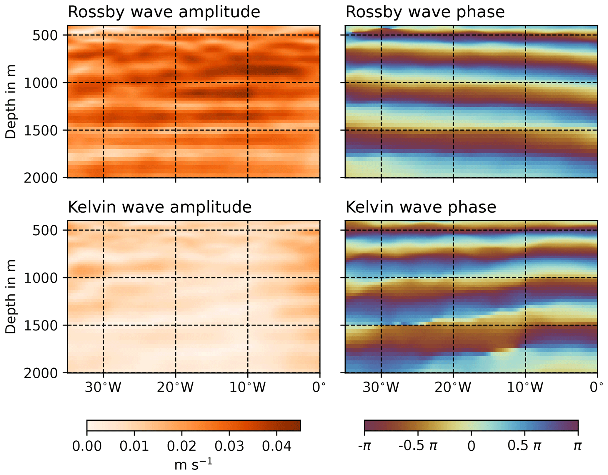
Figure 6 Regression of the vertically filtered (modes 15 to 22) zonal velocity from L200-WIND on the zonal velocity signature of an equatorial Kelvin and a first-meridional-mode Rossby wave of vertical mode 19 and the EDJ frequency. The amplitude shown on the left is the amplitude on the Equator.

3.2 Contributions of Kelvin and first-meridional-mode Rossby waves to the EDJ basin mode

In Fig. 6, a regression of the vertically filtered (containing only vertical modes 15 to 22) zonal velocity between 4^∘ S and 4^∘ N from the wind-driven, flat-bottomed L200-WIND on the zonal velocity signature of an analytic equatorial Kelvin and an analytic first-meridional-mode Rossby wave of vertical mode 19 at the EDJ frequency is shown. The meridional profiles of the two waves have been stretched meridionally before the regression for every model separately to account for the different meridional widths of the EDJs. For more details, see the “Analysis methods” section. It can be seen in Fig. 6 that the Rossby wave has a much larger amplitude at the Equator than the Kelvin wave in L200-WIND. This is consistent with observations of the Atlantic EDJs (Youngs and Johnson, 2015; Bastin et al., 2022). The phase fields of the waves are smooth and correctly show westward propagation for the Rossby wave and eastward propagation for the Kelvin wave, which indicates that the separation of the two wave components by the regression seems to work well. Additionally, the phase difference between the two waves varies approximately linearly with longitude between −π at one boundary and π at the other boundary for all models (not shown), consistent with the theoretical phase difference of the Kelvin wave and the first-meridional-mode Rossby wave in a resonant equatorial basin mode (Cane and Moore, 1981).

To quantify the ratio between the Kelvin and first-meridional-mode Rossby wave amplitudes, the amplitude fields from the regression are averaged between 500 and 2000 m depth and between 25^∘ W and 15^∘ W, where the total EDJ amplitude is strongest and also all other width analyses in this study are performed. The resulting equatorial amplitude values of the two waves are shown for each model in the left panel of Fig. 7, together with the amplitude contributions of the Kelvin and first-meridional-mode Rossby wave to the real Atlantic EDJ basin mode at 1000 m depth as estimated from Argo float data by Bastin et al. (2022). In the centre panel, the amplitude ratio is shown. Again, the model configurations are sorted by the mean meridional width of their EDJs; no systematic relationship between the amplitude ratio and mean EDJ width is visible. In the right panel, the cross-equatorial width of a theoretical basin mode is shown, consisting of an equatorial Kelvin and a first-meridional-mode Rossby wave with the amplitude ratio shown in the centre panel and the phase difference derived by Cane and Moore (1981) but without any higher-meridional-mode Rossby waves. As expected, a larger relative contribution of the Kelvin wave (smaller ratio in the centre panel) leads to a wider EDJ basin mode, but the effect is very small for the ratios derived from the model solutions and also from Argo data. The differences in the Kelvin wave amplitude compared to the Rossby wave amplitude can thus be rejected as a possible explanation for the differences in the mean meridional EDJ width in the models.

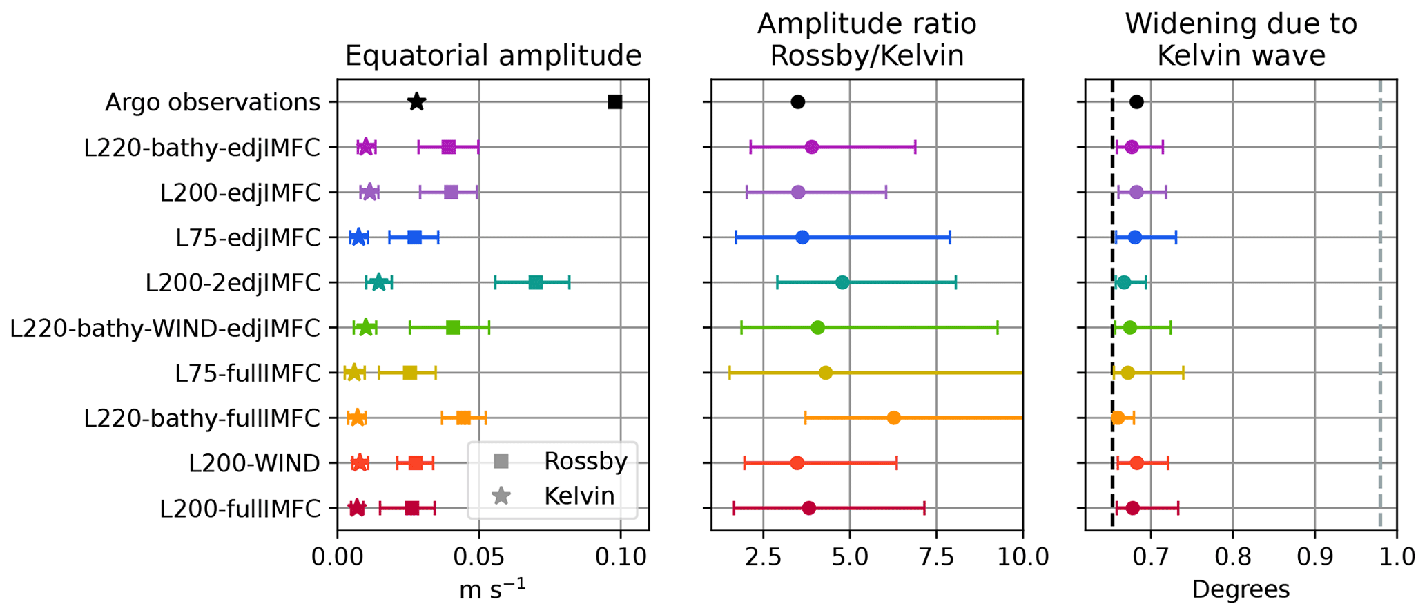
Figure 7 Amplitudes of equatorial Kelvin wave and first meridional Rossby wave contributions to the EDJs for each of the nine models with EDJs, as determined by a regression of the waves' zonal velocity signatures on the vertically filtered (modes 15 to 22) zonal velocity field from the models and averaged between 400 and 2000 m depth and over all longitudes excluding 7.5^∘ at the western and eastern boundary. The models are sorted by their mean EDJ width, from smallest to largest as in Fig. 5. The error bars mark the 68 % quantile of the amplitude distribution from the different longitudes and depths. Also shown in black are the amplitudes of the waves in the real EDJs, as determined from Argo float data by Bastin et al. (2022). Shown in the right panel by the coloured markers is the cross-equatorial width of a theoretical basin mode with the amplitude ratio from the central panel and with higher-meridional-mode Rossby waves neglected. Again, the width (width enhanced by 1.5) of the Rossby wave is marked by the black dashed line (grey dashed line).

There are a few interesting points to note here that are not related to the cross-equatorial width of the EDJs. In general, the EDJs in the models are much weaker than in the real Atlantic Ocean, as visible in the left panel of Fig. 7. One possible reason for this is that the intraseasonal variability exciting and maintaining the EDJs (Ascani et al., 2015; Greatbatch et al., 2018; Bastin et al., 2020) is too weak in the model because of the steady or missing wind forcing and thus less instability in the upper-ocean currents. However, the amplitude ratio of the Rossby and Kelvin wave is quite realistic in many of the model solutions, although in a few the Rossby wave is even more dominant than in reality. It is intriguing that the models, despite their high degree of idealisation, correctly simulate the larger Rossby wave amplitude compared to the Kelvin wave amplitude because this large ratio seems to be a peculiarity of the EDJs in the Atlantic Ocean: Youngs and Johnson (2015) report that in the Indian Ocean and Pacific Ocean the Kelvin and first meridional Rossby waves have similar amplitudes. It is not clear where this difference comes from. Possible reasons might include differences in the ocean basin bathymetry or in the structure of the coastlines. However, because the amplitude ratio is so close to that of the real Atlantic EDJs in our model runs with both rectangular geometry and realistic Atlantic geometry, our results suggest that it might rather be the similar amplitudes of Kelvin and Rossby waves in the Indian and Pacific EDJs that are exceptional instead of the Atlantic EDJ characteristics with the dominant Rossby wave component.

3.3 Importance of meandering and dissipation for EDJ width and connection to intraseasonal meridional velocity variability

According to the theory of Muench et al. (1994), the EDJ widening could be attributed to time averaging over meandering EDJs. Greatbatch et al. (2012), on the other hand, proposed that the EDJs are wider than an inviscid basin mode of corresponding vertical scale because of strong dissipation of momentum compared to weak diapycnal mixing of density around the Equator. In this section, we will separate and quantify the contributions of these two processes to the EDJ widening in the different model runs.

Additionally, we will investigate the relationship between the strength of intraseasonal variability and EDJ width in the model runs because both Muench et al. (1994) and Greatbatch et al. (2012) mention intraseasonal waves in particular as a possible reason for the enhanced EDJ width. Muench et al. (1994) suggest that the EDJ meandering is caused by meridional advection by intraseasonal waves, and Greatbatch et al. (2012) mention small-scale velocity fluctuations associated with intraseasonal waves as a possible source of momentum dissipation. However, for the theory of Greatbatch et al. (2012) other processes could also play a role in contributing to enhanced dissipation of momentum, and more recently it has been shown that intraseasonal waves actually lead to a net positive energy influx into the EDJs, thereby maintaining the jets against dissipation rather than weakening them (Greatbatch et al., 2018; Bastin et al., 2020). Therefore, we would expect the strength of the intraseasonal variability to contribute to the meandering of the EDJs as suggested by Muench et al. (1994), but not so much to the widening of the EDJs through dissipation.

The strength of the intraseasonal variability at depth shows large differences across the nine model configurations that can simulate EDJs. In Fig. 8, spectra of the meridional velocity at the Equator and 23^∘ W are shown for moored observations and two example model configurations, L200-WIND and L200-edjIMFC, which have relatively wide and narrow EDJs, respectively. We use the meridional velocity here to quantify the strength of the intraseasonal variability because it consists mostly of Yanai waves, which only have a meridional velocity component at the Equator. It can be seen that the intraseasonal variability at depth is a bit too weak in L200-WIND compared to observations. One reason for this is probably the missing seasonal cycle in the model's wind forcing because in reality the generation of intraseasonal waves in the tropical Atlantic Ocean is strongest in boreal summer when the shear instabilities between the surface currents intensify (e.g. von Schuckmann et al., 2008). In L200-WIND, this peak generation of intraseasonal variability is missing because of the steady forcing. Another difference is a shift of the maximum spectral power between 1000 and 2000 m depth towards longer periods of about 50 d in L200-WIND compared to 30–40 d in the moored observations. Nevertheless, L200-WIND shows, as do the moored observations, significant spectral power of the intraseasonal meridional velocity variability on the Equator down to depths of at least 3000 m. In contrast to that, L200-edjIMFC shows very reduced equatorial meridional velocity variability on all timescales, also in the intraseasonal period range between 30 and 90 d. This is due to the missing wind forcing in this model configuration. Still, there is an intraseasonal peak in the spectrum at a period of about 70 d.

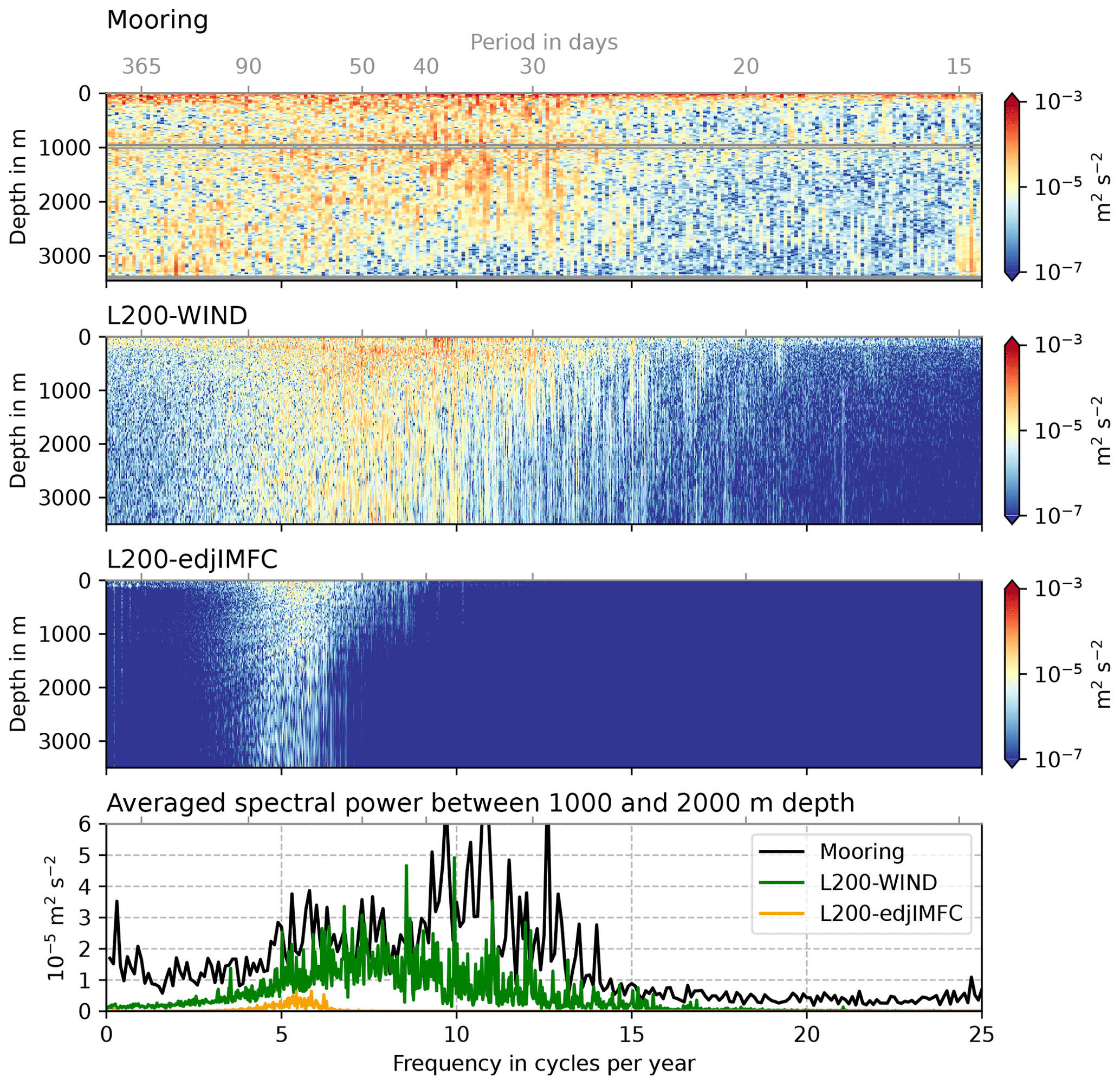
Figure 8 Comparison of power spectra of the meridional velocity in moored observations and two model runs at 0^∘ N, 23^∘ W. The top panel has been updated and modified from Tuchen et al. (2018) using extended time series (2001–2021) from Tuchen et al. (2022a).

The averaged spectral power of the equatorial intraseasonal meridional velocity variability is shown for each of the nine model configurations in Fig. 9 (centre left panel). Again, the models are sorted by their mean meridional EDJ width, which is also shown in the left panel of the figure for comparison.

To separate the reversible (meandering) and the irreversible (widening by dissipation) part of the EDJ widening in the model, a Gaussian bell curve is fitted to the vertically filtered (modes 15 to 22) zonal velocity at 1000 m depth, at every longitude between 25 and 15^∘ W, and every point in time separately. The mean width due to meandering, as well as the width due to dissipation, is then estimated from the fit parameters as described in Sect. 2.2. In Fig. 9, the resulting meridional widths for each of the nine model configurations are shown in the centre right panel for meandering and in the right panel for dissipation. Again, the width (width enhanced by 1.5) of the Rossby wave is marked by the black dashed line (grey dashed line) to give an impression of what fraction of the observed mean EDJ widening can be achieved by the process in question. It can be seen that there are differences between the model configurations in how much the EDJs meander. Not surprisingly, the model runs with wind forcing or full intraseasonal momentum flux convergence forcing, which also have more intraseasonal variability, show more meandering of the EDJs. In the four model configurations with the largest mean EDJ widths, the meandering widens the EDJs in the time mean by about half the observed widening of a factor of 1.5 and in L75-fullIMFC even more. Our model results thus suggest that meandering of the EDJs does play a role in widening the EDJs meridionally in the time mean. The width due to dissipation of the EDJs is also larger in the model runs with wind forcing or full IMFC forcing, again consistent with the enhanced intraseasonal variability in those models (although here the relationship is not that clear; more details follow in the next paragraph). Except for L75-fullIMFC, the widening by dissipation explains a larger part of the observed EDJ widening than the meandering, with the width due to dissipation of the EDJs in L200-WIND and L200-edjIMFC even reaching a factor of 1.5 compared to the theoretical Rossby wave scale.

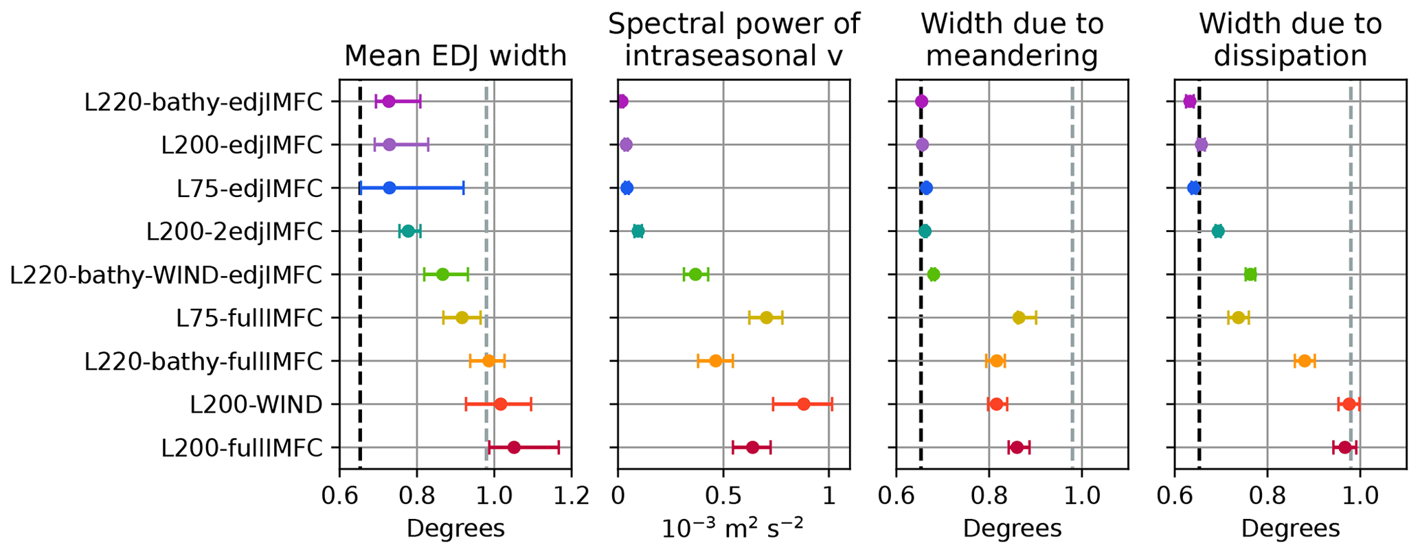
Figure 9 Contributions to mean meridional EDJ width by meandering and widening by dissipation. Left panel: mean meridional EDJ width, as shown in Fig. 5. Centre left panel: spectral power of the equatorial intraseasonal meridional velocity averaged over periods of 30 to 90 d, between 400 and 2000 m depth, and over all longitudes excluding 7.5^∘ at the western and eastern boundary. The intraseasonal spectral power has been estimated using Welch's method, and the error bars show the 68 % quantile of the spectra from the different segments. Centre right panel: time mean width of a theoretical Rossby wave meandering with the same distribution of velocity core shifts away from the Equator as determined for the model in question. Right panel: meridional width of the EDJs due to dissipation. For the last two panels, the uncertainty has been estimated using bootstrapping (redoing the analysis on randomly chosen subsamples of the entire dataset). Again, the 68 % quantiles are marked. The width (width enhanced by 1.5) of the Rossby wave is marked by the black dashed line (grey dashed line).

As expected, a clear relationship between the strength of the intraseasonal variability and the EDJ meandering can be seen in Fig. 9. Also, the EDJ width due to dissipation is generally larger in the models with more intraseasonal variability. To investigate and quantify this, linear regressions of the mean width of the EDJs due to the two processes onto the averaged spectral power of the equatorial meridional velocity variability are shown in Fig. 10. For both processes, there is a positive correlation between the meridional EDJ width and the strength of the intraseasonal variability. In the case of the EDJ meandering, the correlation is quite large, and the regression can explain 81 % of the variance in mean EDJ width due to meandering. This is consistent with the suggestion of Muench et al. (1994) that the meandering is caused by meridional advection through intraseasonal waves. For the EDJ width due to dissipation, the correlation is smaller, but 73 % of the variance can still be explained by the regression on the strength of the intraseasonal variability. This connection is surprisingly large given the more recent finding that intraseasonal waves actually maintain the EDJs rather than dissipate them (Greatbatch et al., 2018; Bastin et al., 2020). We suspect that the large correlation is due to the generally enhanced level of variability in the models with larger intraseasonal spectral power such that other processes dissipating the EDJs are also stronger. According to the theory by Greatbatch et al. (2012), these could be all the processes that lead to loss of momentum, i.e. cause a negative power input into the EDJs.

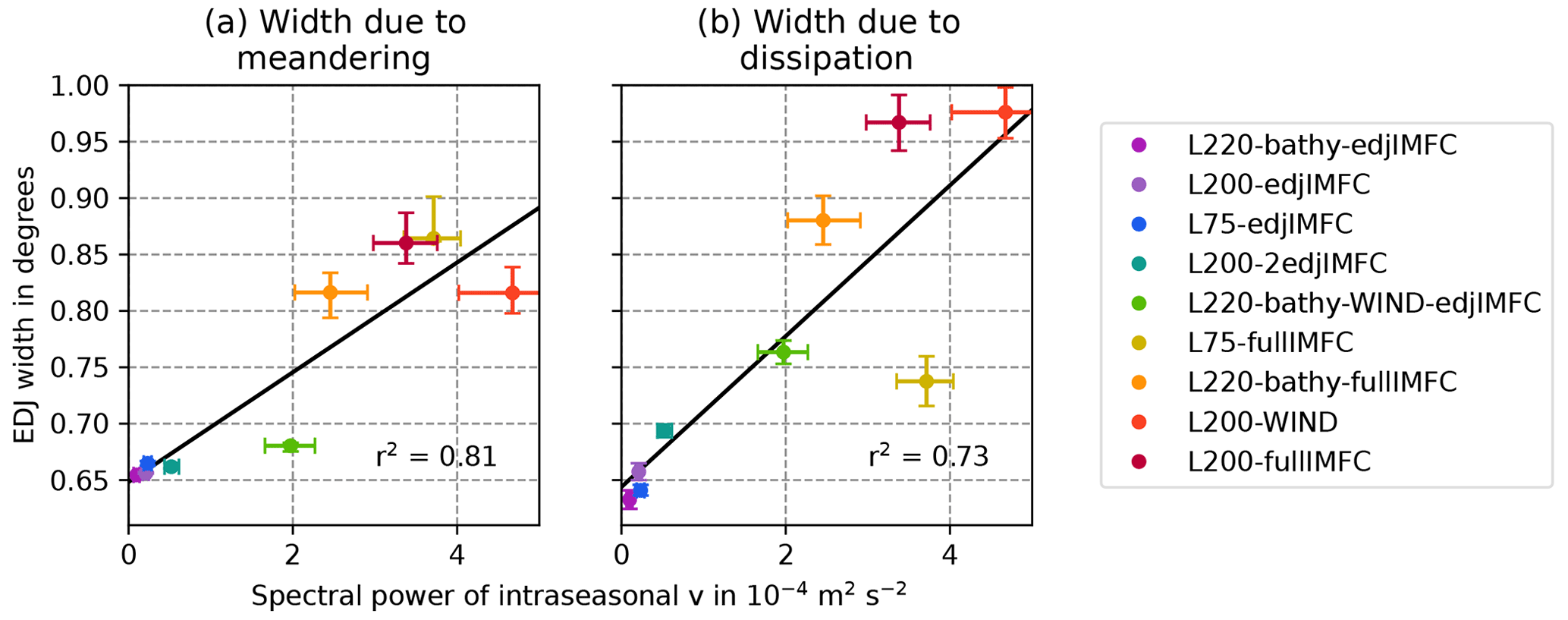
Figure 10 Relation between the strength of intraseasonal meridional velocity variability and the enhanced mean meridional width through meandering (a) or widening by dissipation (b) of the EDJs in the models. The spectral power of the equatorial meridional velocity has been averaged over all longitudes excluding 7.5^∘ at the western and eastern boundary, between 400 and 2000 m depth, and between periods of 30 and 90 d. Error bars mark the 68 % quantile of the parameter distribution obtained by Welch's method (for the intraseasonal spectral power) and bootstrapping (for the EDJ width due to meandering or dissipation). Shown in black is a linear regression, with the squared correlation coefficient r² indicated in the lower right corner.

4 Conclusions and discussion

In this study, it could be shown that widening by irreversible mixing processes or momentum loss plays a larger role in setting the enhanced time mean meridional width of the EDJs than time averaging over meandering of the jets. It thus seems that the theory suggested by Greatbatch et al. (2012), which attributes the enhanced meridional EDJ width to large dissipation or loss of momentum compared to small diapycnal mixing of density, is the main factor for the observed widening of the EDJs. Nevertheless, meandering of the EDJs around the Equator also contributes non-negligibly to the meridional widening of the EDJ time mean amplitude field, as suggested by Muench et al. (1994).

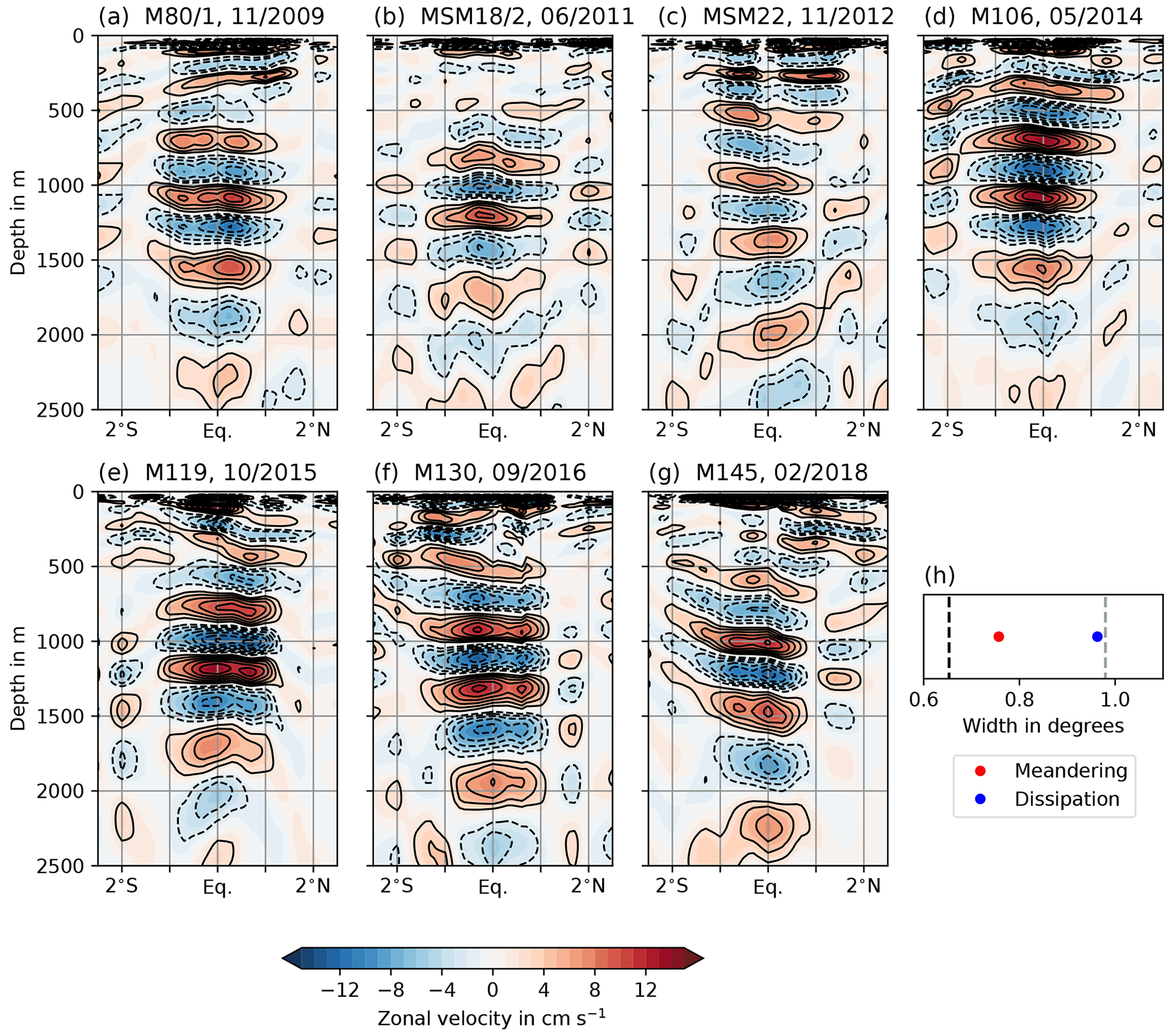
Figure 11 Zonal velocity sections measured during seven different cruises along 23^∘ W. Panels (a) to (g) show the filtered zonal velocity, containing only vertical modes 14 to 20 corresponding to the Atlantic EDJs. Black contours are drawn every 2 cm s⁻¹; solid is for eastward and dashed for westward velocity. (h) The mean values of EDJ width due to dissipation or momentum loss and width due to averaging over meandering jets are shown, again together with the Rossby wave width (black dashed line) and 1.5 times the Rossby wave width (grey dashed line).

However, the results shown here are based only on idealised model simulations of the EDJs. The exact magnitude of the contributions of both suggested processes in the real ocean cannot be inferred from these model experiments, but it is possible to gain some insight by looking at ship sections of the EDJs. In general, the width of the EDJs has been determined from observations by looking at time mean sections (e.g. Muench et al., 1994) or by spectral analysis, which also gives a time mean width (e.g. Johnson and Zhang, 2003; Youngs and Johnson, 2015), such that it is not possible to distinguish between the widening by meandering and widening by dissipation or momentum loss. By looking at synoptic (i.e. measured in the course of a few days) zonal velocity sections, it is possible to assess whether the real EDJs show both an enhanced width due to dissipation or momentum loss and due to meandering as in the model results presented in this study.

In Fig. 11, zonal velocity sections at 23^∘ W are shown, which were measured during several cruises conducted in the framework of the research project SFB 754, Climate–Biogeochemistry Interactions in the Tropical Ocean (Krahmann and Mehrtens, 2021; Krahmann et al., 2021). The data have been filtered by decomposing them into vertical normal modes and keeping only modes 14 to 20, approximately corresponding to the EDJ peak, to remove variability different from the EDJs. The normal mode decomposition has been done using a mean stratification profile from several cruises as described in Claus et al. (2016). To these filtered data, a Gaussian curve has been fitted at all depths between 500 and 2000 m where the maximum velocity exceeds 5 cm s⁻¹, and the width due to dissipation and width through meandering have been calculated as described in Sect. 2.2. In the cruise data, the width due to dissipation or momentum loss of the EDJs contributes about 3 times as much as averaging over meandering jets to the excess EDJ width compared to the theoretical Rossby wave profile, which corroborates our results from the set of idealised model experiments.

Similar synoptic zonal velocity sections of the Atlantic EDJs from different longitudes and times, measured during EQUALANT cruises in 1999 and 2000, are shown by e.g. Gouriou et al. (2001), Bourlès et al. (2003), and Bunge et al. (2006). They also show wider EDJs and only small shifts of the jet cores away from the Equator. These observations support the conclusion that widening by momentum loss e.g. due to irreversible mixing processes, which can be explained by enhanced dissipation and/or loss of momentum together with small diapycnal mixing of density (Greatbatch et al., 2012), plays the most important role in setting the enhanced mean cross-equatorial width of the Atlantic EDJs, whereas averaging over meandering of the jets as suggested by Muench et al. (1994) provides a smaller contribution to the enhanced mean EDJ width.

It has been suggested that the time mean circulation flanking the EDJs contributes to their enhanced cross-equatorial width by shielding the Equator from the effect of Rossby waves that are generated off the Equator (Claus et al., 2014). Unfortunately we cannot assess the contribution of that process for the EDJ width in this study because the strength of the flanking mean flow in our idealised model simulations is connected to the presence or absence of wind forcing, and its effect is thus overlain by that of other wind-driven variability, leading to more dissipation. However, Claus et al. (2014) found that the effect of the flanking mean flow on the EDJ width is much smaller than that of enhanced eddy viscosity, which is consistent with our result that momentum dissipation is the most important factor controlling the EDJ width.

Another interesting result from the model experiments shown here is the connection of the meridional EDJ widening to the strength of intraseasonal variability in the depth range of the EDJs. From the models, it can be concluded that the meandering of the EDJs is very likely largely due to meridional advection of the EDJs by intraseasonal waves, as suggested by Muench et al. (1994). A linear regression of the mean EDJ width due to meandering on the spectral power of the intraseasonal meridional velocity variability in the depth range of the EDJs yields an explained variance of 81 %. This is slightly less for the part of the mean EDJ widening that is due to widening by dissipation or momentum loss of the EDJ basin mode, whereby a regression on the spectral power of the intraseasonal variability can explain 73 % of the variance. This in surprisingly large because although Greatbatch et al. (2012) mention intraseasonal meridional velocity fluctuations in particular as a possible source for the enhanced dissipation of EDJ momentum, it was later shown that intraseasonal waves in fact maintain the EDJs instead of dissipating them (Greatbatch et al., 2018; Bastin et al., 2020). Hence, for the EDJ widening by dissipation or momentum loss, other processes and variability on other timescales have to be mainly responsible. The EDJs not only lose momentum through dissipation, but also transfer energy to the time mean flow (Ascani et al., 2015; Bastin et al., 2020), which probably contributes to the widening of the EDJs. Among possible sources of momentum dissipation of the jets is their interaction with the Equatorial Undercurrent (EUC). Another possible source of enhanced momentum dissipation in the EDJs could be inertial instability, which could take place in particular in the westward jets of the EDJs as was suggested by Ménesguen et al. (2009). However, inertial instability would also involve vertical mixing of density, which has been shown to be very weak at the Equator below the EUC (Dengler and Quadfasel, 2002; Gregg et al., 2003) and which furthermore has to be weak compared to the momentum dissipation for the geostrophic jets to widen (Greatbatch et al., 2012). Further research is necessary to identify and quantify the impact of these and other sources of momentum loss for the EDJs.