the Creative Commons Attribution 4.0 License.
the Creative Commons Attribution 4.0 License.
 | 22 Jun 2023
Unsupervised classification identifies coherent thermohaline structures in the Weddell Gyre region
Maike Sonnewald
Shenjie Zhou
Ute Hausmann
Andrew J. S. Meijers
Isabella Rosso
Lars Boehme
Michael P. Meredith
Alberto C. Naveira Garabato
The Weddell Gyre is a major feature of the Southern Ocean and an important component of the planetary climate system; it regulates air–sea exchanges, controls the formation of deep and bottom waters, and hosts upwelling of relatively warm subsurface waters. It is characterised by low sea surface temperatures, ubiquitous sea ice formation, and widespread salt stratification that stabilises the water column. Observing the Weddell Gyre is challenging, as it is extremely remote and largely covered with sea ice. At present, it is one of the most poorly sampled regions of the global ocean, highlighting the need to extract as much value as possible from existing observations. Here, we apply a profile classification model (PCM), which is an unsupervised classification technique, to a Weddell Gyre profile dataset to identify coherent regimes in temperature and salinity. We find that, despite not being given any positional information, the PCM identifies four spatially coherent thermohaline domains that can be described as follows: (1) a circumpolar class, (2) a transition region between the circumpolar waters and the Weddell Gyre, (3) a gyre edge class with northern and southern branches, and (4) a gyre core class. PCM highlights, in an objective and interpretable way, both expected and underappreciated structures in the Weddell Gyre dataset. For instance, PCM identifies the inflow of Circumpolar Deep Water (CDW) across the eastern boundary, the presence of the Weddell–Scotia Confluence waters, and structured spatial variability in mixing between Winter Water and CDW. PCM offers a useful complement to existing expertise-driven approaches for characterising the physical configuration and variability of oceanographic regions, helping to identify coherent thermohaline structures and the boundaries between them.
- Article
(30302 KB) - Full-text XML
- BibTeX
- EndNote


The Southern Ocean is a key region in the global climate system, hosting crucial transformations that supply waters to both the upper and lower limbs of the global ocean overturning circulation (IPCC, 2022, chap. 3). The lower limb is renewed by dense waters that form and are exported northward, flooding the majority of the global abyssal ocean (Johnson, 2008). The Weddell Sea is important for this dense water production and export, with its southern and western continental shelves hosting interactions with floating ice shelves, as well as strong cooling and sea ice production in polynyas (Vernet et al., 2019). These exchanges result in shelf waters that are extremely cold (some below the surface freezing point) and comparatively saline; this gives them sufficient density to spill from the shelf down the slope and into the deep Weddell Sea, entraining mid-depth waters as they descend (Foster and Carmack, 1976; Gill, 1973; Killworth, 1983; Gordon et al., 2001).
In addition to this mode of deep-ocean ventilation, sporadic occurrences of deep convection over the deep Weddell Sea have been observed, especially in the vicinity of Maud Rise. Here, large-scale polynyas can emerge that enable dense water production and sinking; this was first noted in the 1970s (Gordon, 1978), with indications that this may have recently recurred after a decades-long hiatus (Campbell et al., 2019). The dense waters that form in the Weddell Sea penetrate northwards to supply the lower limb of the Atlantic Meridional Overturning Circulation. There are signs that this export has been dwindling in recent years (Johnson et al., 2008), though hiatuses in the decline have been noted (Abrahamsen et al., 2019). To reach the Atlantic, the dense water must navigate the complex bathymetry of the Scotia Arc, the southern flank of which comprises the South Scotia Ridge. The most direct route for dense water to cross this ridge is Orkney Passage (Naveira Garabato et al., 2002), though the possibility of significant outflow around the outside of the Scotia Arc also exists (Jullion et al., 2014).
The Weddell Gyre region is a complex nexus of circumpolar and gyre circulation, with ubiquitous water mass formation and transport (Fig. 1). Horizontal circulation to the north of the gyre is dominated by the Antarctic Circumpolar Current (ACC), the eastward-flowing current system that comprises several discrete fronts and which is characterised by strong spatial variability (Sokolov and Rintoul, 2009; Rintoul and Garabato, 2013). The Weddell Gyre separates the ACC from Antarctica in the Atlantic sector; it is a cyclonic circulation system that extends east from the eastern Antarctic Peninsula. No topographic or distinct current feature forms its eastern extent, but it is nominally placed at approximately 30∘ E or even further eastwards. In the meridional direction, it extends from the continental slope to approximately 60∘ S (Fahrbach et al., 1994; Park et al., 2001; Meijers et al., 2010; Vernet et al., 2019). At its eastern flank, the voluminous mid-depth Circumpolar Deep Water (CDW) from the ACC is entrained into the Weddell Gyre, where it mixes to become cooler and fresher, and is usually termed Weddell Deep Water or Warm Deep Water (WDW) (Fahrbach et al., 1994). This is the oceanic source that penetrates onto the shelf and is modified to become the dense waters that ultimately flow northward at depth (Jullion et al., 2014; Naveira Garabato et al., 2016). Circulation within the gyre exhibits a two-cell structure, with the western cell centred around 40∘ W and the eastern gyre centred around 18∘ E (Reeve et al., 2019). The gyre is forced by westerly winds over its northern edges, producing upwelling in its centre; it is also forced by easterly winds over its southern edges, producing downwelling along its southern limb (Naveira Garabato et al., 2016). In addition, it is subject to strong buoyancy forcing. Separating the ACC to the north from the Weddell Gyre to the south, the Weddell–Scotia Confluence (WSC) follows close to the complex bathymetry of the South Scotia Ridge (Fig. 1). The WSC is identifiable from the waters on either side by characteristically low stratification at mid-depths; this has been ascribed to the injection and sinking of shelf waters from the tip of the Antarctic Peninsula (Fig. 1).
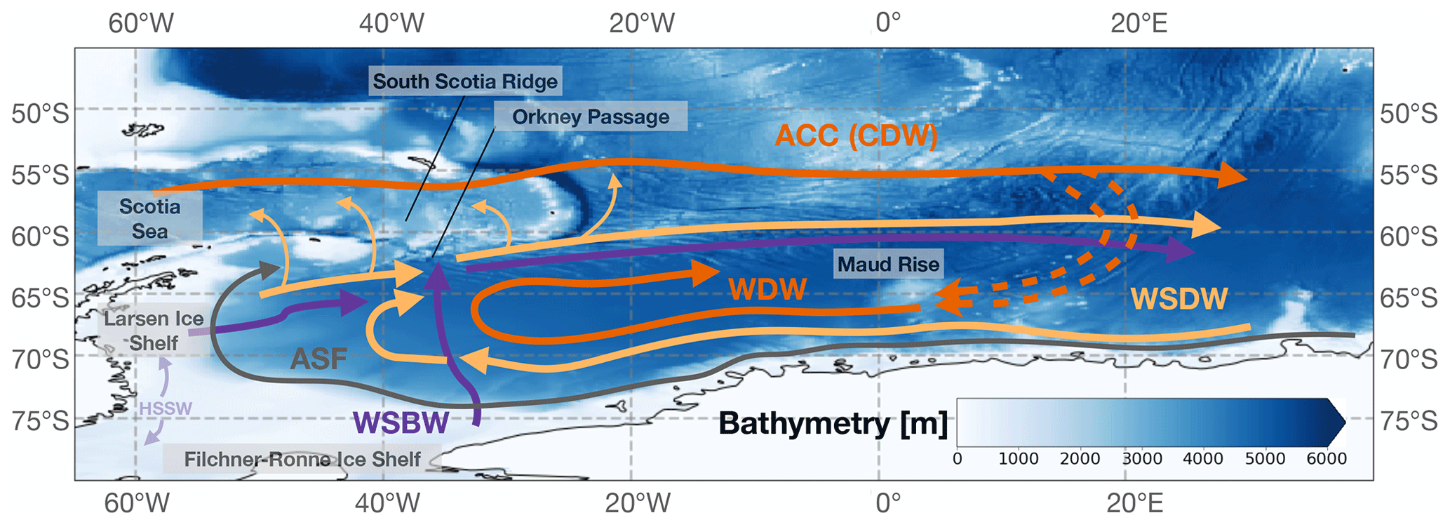
Figure 1Schematic of the circulation of the Weddell Gyre region. The broad circulation features include the Antarctic Circumpolar Current (ACC), Circumpolar Deep Water (CDW), Weddell Sea Deep Water (WSDW), Warm Deep Water (WDW), Weddell Sea Bottom Water (WSBW), High-Salinity Shelf Water (HSSW), and the Antarctic Slope Front (ASF). Selected geographic features are named, and the colour scale shows the bathymetry. Adapted from Vernet et al. (2019).
Despite the importance of the Weddell Gyre and its surroundings, its structure and dynamics are not thoroughly understood, partly because of the practical difficulties in observing the region. It is remote and inaccessible, especially in winter when it is extremely challenging to reach by ship, and it is frequently covered by clouds and long periods of darkness, making it challenging to acquire complete satellite observations in the visible spectrum. These limitations underscore the importance of making the most of the sparse data that we do have using a wide variety of observational analysis and reanalysis techniques (e.g. Reeve et al., 2016). One way to extract additional value from existing data is to employ unsupervised classification, a broad suite of methods for finding coherent patterns in unsorted or uncharacterised data, to identify and characterise structures within those data.
Unsupervised classification of oceanographic variables
Unsupervised learning attempts to reveal relationships among inputs, often referred to as “features” in machine learning terminology. Using these algorithms, researchers can identify sub-populations in data distributions and find hidden covariance structures, filtering out random, unstructured noise and gaining insight into potential connections between variables. As a result, it has become a valuable tool in a variety of fields, including oceanography (Sonnewald et al., 2021). For example, Sonnewald et al. (2019) identified coherent dynamical regimes in the global ocean by using the terms of the barotropic vorticity budget as the “features” or “dimensions” of the unsupervised classification analysis. Jones and Ito (2019) applied a similar method to the surface carbon budget in a numerical model, and Sonnewald et al. (2020) used a multi-layered unsupervised classification approach to identify ecological regimes. Couchman et al. (2021) applied unsupervised learning to cluster fluid patches according to their background buoyancy frequency and turbulent dissipation rates. Because the “decisions” made by many of these unsupervised classification approaches are somewhat transparent and can be thoroughly analysed, at least when the complexity of the model is kept at a manageable level, unsupervised classification results are often interpretable by oceanographic experts, highlighting their potential for uncovering novel or underappreciated structures in complex, multi-dimensional oceanographic data (Sonnewald and Lguensat, 2021). Generally speaking, unsupervised classification can be thought of as a “hypothesis generation tool” (Kaiser et al., 2022). For a review of recent machine learning advances in oceanography, including unsupervised classification, see Sonnewald et al. (2021).
In many oceanographic unsupervised classification applications, the dataset consists of a collection of profiles, where a “profile” refers to a set of measurements taken at various pressures at a single location. The measured quantities may consist of temperature, salinity, and biogeochemical variables such as oxygen. Often the applications revolve around identifying different “profile types”, which may also be called classes or groups. There are a variety of unsupervised classification approaches for working with profile data. For example, Thomas and Müller (2022) used a self-organising map approach to group temperature profiles in the European Arctic, in part to facilitate numerical model validation.
One particular unsupervised classification method is the profile classification model (PCM) approach, which is an ocean-specific application of Gaussian mixture modelling (GMM), for identifying the profile types (Maze et al., 2017). In PCM, one attempts to statistically model the profiles, typically as represented in an abstract principal component space, as a collection of multi-dimensional Gaussian functions. The result is a set of profile types that feature similar vertical structures across one or more measured quantities (e.g. with temperature and salinity data both contributing to the identification of the profile types).
PCM has been used in a number of applications in recent years. Jones et al. (2019) applied the PCM approach to Southern Ocean temperature profile data, identifying spatially coherent regimes that roughly align with modern understanding of Southern Ocean fronts and subtropical structure. PCM was able to identify these regions despite the fact that it was not given any location information about the profiles. Rosso et al. (2020) expanded this analysis to include salinity in the Indian sector of the Southern Ocean, identifying frontal zones and the variability of water masses present in each zone. Houghton and Wilson (2020) applied PCM to Pacific Ocean temperature data, connecting the temporal evolution of the tropical classes to the El Niño–Southern Oscillation (ENSO), thereby deriving a novel ENSO proxy. Sambe and Suga (2022) applied PCM to the northwestern Pacific Ocean, allowing them to link the variability of the Kuroshio extension to the regional vertical structure. Recently, Xia et al. (2022) used PCM to identify three different types of Antarctic Intermediate Water (AAIW) and their formation regions. PCM may also be useful for finding circulation pathways; Boehme and Rosso (2021) used PCM to identify separate warm and cold modes of transport on the Amundsen Sea shelf. Desbruyères et al. (2021) used an approach called ocean profile clustering to separate subpolar waters from subtropical waters in the North Atlantic, enabling a data-driven analysis of the cooling-to-warming transition of the subpolar North Atlantic. PCM has also been applied to temperature profile quality control, extending its usefulness into a new area (Zhang et al., 2022).
Chapman et al. (2020) challenged oceanographic researchers to rethink our treatment of boundaries and fronts, arguing that a more locally tailored, application-specific, and perhaps even probabilistic approach may be more suitable than attempting to identify a single global set of boundaries between oceanic thermohaline and biogeochemical structures. Because PCM identifies profile types in a probabilistic way, returning a set of probabilities across the profile types, it can be used to reframe how we describe boundaries between oceanographic structures. To this end, Thomas et al. (2021) introduced a method for defining boundaries in a probabilistic fashion using PCM. This quantity, called the inter-class comparison metric (I-metric), uses the difference between the class with the highest probability and the runner-up to quantify the likelihood that a given profile is on the boundary between two classes. Given the ambiguity of the precise extent of the Weddell Gyre, the I-metric approach is a suitable framework for rethinking the boundaries between components of the gyre and its surroundings. We will apply I-metric analysis to the Weddell Gyre profile dataset in this paper.
Thanks to the EU-funded SO-CHIC project, the Southern Ocean research community now has a unified profile dataset that covers the Weddell Gyre and adjacent regions, assembled from various sources (Jones and Zhou, 2022). This dataset has been curated and quality-controlled, and it is of sufficient size to allow unsupervised classification to be useful. In this study, we apply the PCM technique to this newly curated dataset to identify coherent regimes in temperature and salinity structure in the Weddell Gyre region, with the aim of refining our understanding of the area and generating new hypotheses for further investigation. PCM is suitable because it robustly and automatically groups profiles together into classes, allowing for the identification of coherent regimes in thermohaline structure in a probabilistic fashion.
The structure of this paper is as follows. In Sect. 2, we describe the profile dataset and the unsupervised classification method used to identify coherent structures in the data. In Sect. 3, we examine the distribution properties across the four-class PCM, including how those properties vary seasonally. Finally, in Sect. 4, we discuss these results in the context of the literature on the Weddell Gyre and its environs.
2.1 Description of the Weddell Gyre profile dataset
For this study, we used a set of temperature and salinity profiles from the Atlantic and Indian sectors of the Southern Ocean. The dataset consists of profiles taken by Argo floats and ship-based conductivity–temperature–depth (CTD) casts as recorded in the World Ocean Database within a box defined by 85–30∘ S, 65∘ W–80∘ E. We only consider profiles with good position and time flags, as well as good temperature, salinity, and pressure measurements with good flags. Duplicated profiles are identified when multiple profiles are found within 24 h over the same 2 km × 2 km grid cell, following Schmidtko et al. (2014), and only one profile within the spatio-temporal window is used. We then used the MITprof toolbox to pre-process the selected profiles, re-gridding them onto standard pressure levels (Forget et al., 2015). This step is necessary because one requirement of PCM and GMM is that the data have a consistent number of “features”, also referred to as “dimensions” in machine learning terminology, throughout the entire dataset. Here, we select a standard pressure grid with 72 vertical levels, with fine enough vertical resolution to preserve temperature and salinity structure while avoiding data gaps at depth at each grid point. The vertical interval varies from 20 dbar at the surface to 100 dbar in the deep ocean. In total, we used 188 885 Argo profiles and 34 915 ship-based CTD profiles covering 20–1000 dbar for the initial classification step, i.e. the identification of near-Antarctic waters. We first used PCM to sort the entire profile dataset into five classes based on their combined temperature and salinity structure. Broadly speaking, these classes may be described as (1) a subtropical Atlantic sector class, (2) a subtropical Indian sector class, (3) a more northern circumpolar class, (4) a more southern circumpolar class, and (5) a near-Antarctic class that sits roughly south of the Polar Front (PF, Appendix B). One could obtain a similar sub-Antarctic class by simply selecting all profiles located south of the PF. Because we are primarily interested in the Weddell Gyre and its surroundings, we chose to focus on the near-Antarctic class. Effectively, the rest of this paper describes a “sub-classification” of the near-Antarctic class into even smaller groups. This sub-classification might be thought of as a two-level hierarchy in that we are looking for classes within a class. As an extra benefit, focusing our clustering efforts on the near-Antarctic region means that the global data imbalance (i.e. the relative abundance of observations north of the PF) is less likely to bias our results.
The distribution of the near-Antarctic profiles used in the rest of this study features some spatial biases in coverage, which we handle carefully at the training stage (Fig. 2a). The earliest profiles are from CTD casts in the 1970s, although the vast majority of the profiles are from the Argo float era, i.e. from the mid-2000s onward (Fig. 2c). The near-Antarctic profiles are broadly characterised by a near-surface temperature inversion (i.e. colder at the surface and warmer at depth), which is stabilised by the salinity stratification (i.e. fresher at the surface and saltier at depth). Such profiles are often described as “salt-stratified”, indicating that their vertical stability depends on salinity and not temperature (Roquet et al., 2022). The widespread presence of salt stratification in the near-Antarctic class is consistent with the property contrast usually seen across the PF, which acts as an approximate dividing line between waters bearing the imprints of near-Antarctic processes (e.g. ice shelf melting and iceberg calving leading to a layer of near-surface fresh water) and waters bearing the imprints of more subtropical processes.
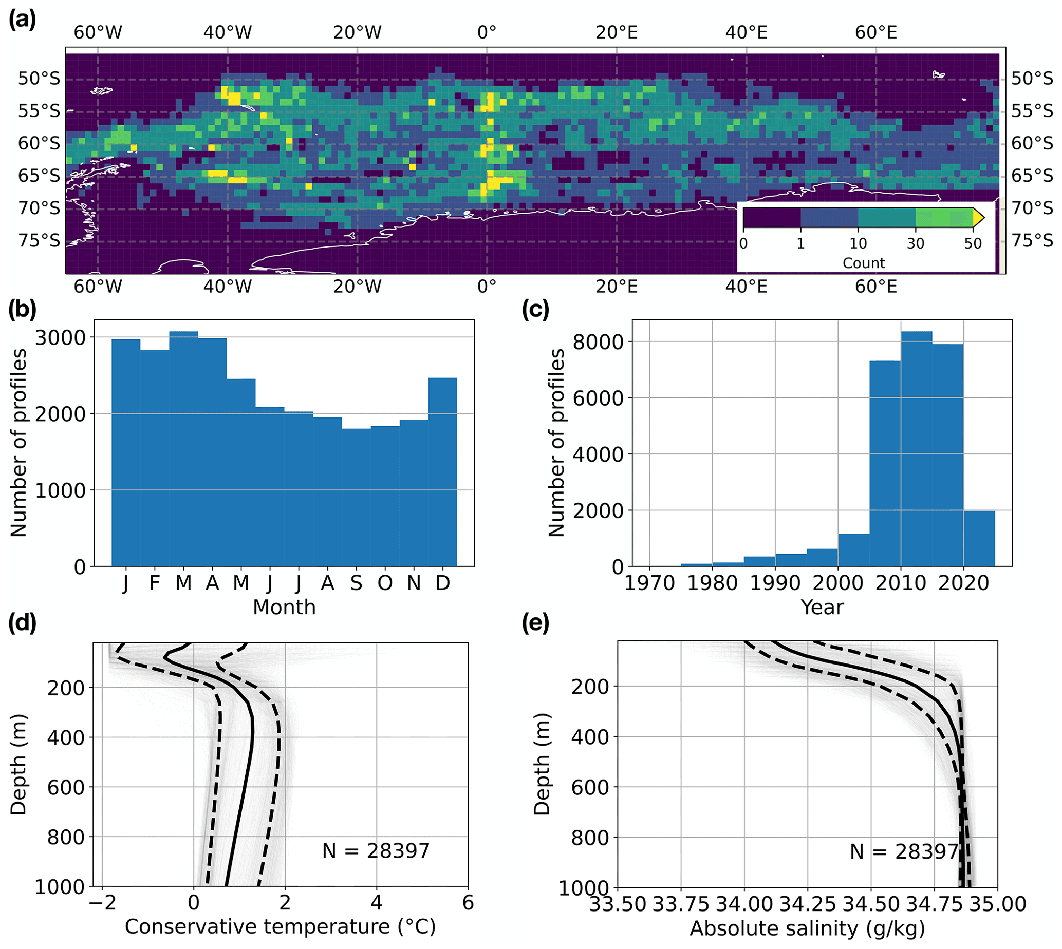
Figure 2The distribution of profiles used in this study. (a) Number of profiles in the dataset shown in 1∘ latitude–longitude bins. Note that profiles with a maximum depth of less than 1000 m have been excluded. (b) Distribution of the profiles by month. (c) Distribution of the profiles in 5-year intervals. (d) Random selection of 10 % of the conservative temperature profiles by depth (thin grey lines), shown with the 25th percentile (thin dashed line, left), the median (solid black line), and the 75th percentile (thin dashed line, right). (e) Same as (d), but for absolute salinity. The total number of profiles is N = 28 397.
2.2 Profile classification modelling as applied to the Weddell Gyre profile dataset
In this section, we use PCM to identify profile types within the near-Antarctic collection of profiles. First, we pre-process the near-Antarctic profiles by standardising the temperature and salinity values on each pressure level. This ensures that, on each pressure level, the temperature and salinity distributions have a mean of zero and a variance of 1.0. The advantage of scaling each pressure level separately is that it allows all variations in temperature and salinity structure to be specified relative to the observed variability on that pressure level. Without such standardisation, variations in the near-surface values, which tend to have a strong seasonal imprint, would dominate the classification and obscure the structural importance of smaller variations at depth.
After standardising the temperature and salinity values on each pressure level, we reduce the dimensionality of the dataset by carrying out principal component analysis (PCA). This reduces the computational complexity of the classification task and effectively filters out some of the small-scale vertical variability in the profiles. PCA may also be used to study ocean structures by itself (e.g. Pauthenet et al., 2017), but here we mainly use it as a dimensionality reduction technique (Appendix A1). We employ a six-component PCA that retains roughly 95 % of the vertical variability in the near-Antarctic profile dataset (Appendix A). PCA reduces the number of “features” in the classification problem from 42 (i.e. temperature and salinity values on 21 pressure levels) to six. It is within this six-dimensional abstract PC space that we wish to identify coherent sub-groups or classes. However, this brings us to a complex issue in unsupervised classification: into how many different classes should we attempt to sort the profiles?
Because oceanographic data are highly correlated across a variety of spatial and temporal scales, they cannot always be cleanly separated into groups. As a result, there is not necessarily an objective measure for the “success” of any particular unsupervised classification approach. Instead, techniques such as the PCM should be considered tools for exploration and discovery within a dataset, allowing us to identify coherent regimes with similar vertical structures and the boundaries between them in a probabilistic fashion. As with many classification problems, there is a trade-off between the complexity of the classification model and its interpretability. Simple two-class models are usually straightforward to interpret (e.g. colder waters versus warmer waters), but they ignore more subtle structures in the data which may be of interest. As we increase the number of classes into which we attempt to sort the data, we often lose interpretability as the classes often become increasingly difficult to distinguish from one another. There are statistical tools that can help guide our choice of the number of classes, aiding us in avoiding the common pitfalls of underfitting and overfitting, but these tools often only provide a range, within which we are free to choose the level of complexity of the statistical model (Appendix A). This is roughly analogous to the “hierarchy of models” concept outlined by Held (2005), which suggests that we can learn a great deal about a system by studying what happens as we add or take away various sources of complexity. In the context of PCM, increasing the number of classes effectively increases the level of complexity of our representation of the system.
For this paper, we will focus on a four-class representation of the near-Antarctic profile dataset. This four-class model is simple enough to be readily interpretable, while being complex enough to identify differences between circumpolar waters, the transition between circumpolar waters and the gyre, the outer gyre, and the central gyre. Classification approaches must strike a balance between interpretability and complexity, and here we found the four-class model to be (1) within the constraints suggested by statistical criteria and (2) sufficiently complex as to allow for a rich description of the system. Decreasing the number of classes to three loses the distinction between the gyre edge and the gyre core. Increasing the number of classes beyond four leads to an increasing amount of overlap between the classes, making them more difficult to interpret (Appendix A). In the next section, we describe the four-class description of the near-Antarctic profile dataset.
3.1 Structure of the classes
The four-class PCM identifies (1) a circumpolar class, (2) a transition class between the circumpolar waters and the Weddell Gyre, (3) waters on the edge of the gyre, and (4) waters in the core of the gyre. We can identify some key differences between the four classes by examining their vertical structures in temperature, salinity, and the resulting density (Fig. 3). All descriptions here are intended to be relative between the four classes. The circumpolar class features a mean temperature distribution that is relatively warm and is characterised by a deep temperature minimum (median depth 120 m, Fig. 3, top row). The layering observed in the top 1000 m consists of alternating warm and cold layers, stabilised throughout by a gently changing salt stratification with fresher water near the surface and saltier water at depth; the resulting density structure is well-stratified. When compared with the circumpolar class, the transition class, which sits between the more circumpolar waters and the more gyre-based waters, is characterised by a shallower temperature minimum (median depth 80 m) and weaker salt stratification in the subsurface. The resulting density structure is slightly less stratified in the subsurface (Fig. 3, second row). The two gyre classes both feature a shallow temperature minimum and two salt regimes: specifically a region of increasing salinity with depth and a region of uniform salinity. The resulting density structures reflect these salinity differences. The gyre edge features a more gradual change between these two salt regimes with depth, whereas the gyre core features a rapid change in salt stratification at around 200 m depth (Fig. 3, bottom two rows). The median depth of the temperature minimum is 80 m for the gyre edge class and 60 m for the gyre core class, which is broadly consistent with the upwelling of CDW within the cyclonic gyre centre. The temperature minimum, which indicates the presence of WW, deepens as we consider classes further away from the gyre core (Fig. 3, from the bottom row to the top row). Specifically, reporting the 25th, 50th, and 75th percentiles, the Winter Water depths are in the range of (20, 60, 80 m) in the gyre core, (20, 80, 100 m) in the gyre edge, (60, 80, 120 m) in the transition class, and (100, 120, 140 m) in the circumpolar class.

Figure 3Distribution of the conservative temperature, absolute salinity, and potential density anomaly (σ0) of the four classes identified by the GMM algorithm. Each panel features a random selection of 1000 profiles (thin grey lines), the 25th percentile (dashed line, left), the median (solid line), the 75th percentile (dashed line, right), and the number of profiles N in each class. The dotted horizontal lines on the leftmost column indicate, for each class, the median depths of the maximum temperature. Each class gets its own colour for easier comparison with other figures.
We find that the four classes occupy fairly distinct regions, with some expected overlap due to the highly correlated nature of ocean data and the probabilistic nature of our classification method (Fig. 4). The mean dynamic height anomaly of the 500 m surface, chosen to give some indication of the “height” structure of the classes, is deepest in the circumpolar class, with a median value of −3.0 m. As we consider the classes from north to south, the broad deep-to-shallow progression of the 500 mb dynamic height surface is consistent with broad upwelling in the gyre and downward-sloping surfaces further north (Fig. 4, top to bottom). The circumpolar class is broadly located between the PF and the southern boundary of the ACC (SBDY), although some circumpolar-class profiles are found south of the SBDY between 20–40∘ E, a fingerprint of the intrusion of CDW into the gyre (Fig. 4a). The intrusion occurs over a broader region than previously thought (Vernet et al., 2019).
The structure of the interval between the Scotia Sea waters, which are in the circumpolar class, and the Weddell Gyre waters is more complex than had previously been appreciated, consisting of a transition regime and a gyre edge class. The transition class straddles the SBDY in the western part of the domain and is more clearly south of the SBDY in the eastern part of the domain, especially east of the Prime Meridian. As with the circumpolar class, this excursion south of the SBDY is another fingerprint of the conversion of ACC-sourced CDW to WDW (Fig. 1). It features shallower dynamic heights (median −2.3 m), although the excursion south of the SBDY has a height gradient.
The gyre edge class features two distinct branches: (1) a northern branch that sits just south of the SBDY and (2) a southern branch consisting of profiles largely along contours near the Antarctic continent, where f=2Ωcos (ϕ) is the Coriolis parameter (Ω is Earth's rotation rate and ϕ is latitude), and h is the depth of the water column. The more northern branch is indicative of the Weddell–Scotia Confluence (WSC) waters, which is a region of reduced mid-layer stratification located near the South Scotia Ridge that separates the Weddell Gyre waters from those of the Scotia Sea (Patterson and Sievers, 1980). The WSC, as identified by PCM, extends further eastward than previously thought (Vernet et al., 2019). When considered together, the two branches may be thought of as largely aligning with the edge of the gyre, where its isopycnals dome down into the subsurface. Its median dynamic height anomaly is −2.0 m, although some regions in its western branch are shallower than the median.
Finally, the gyre core class is characterised by a dynamic height gradient from west to east, with an overall median value of −1.6 m. Although this PCM does not separate the western and eastern cells of the gyre circulation, the shape of the gyre core class reflects the agglomeration of these two, for example in the northeastern excursion between 0 and 20∘ E. The central gyre is more complex than just a single cyclonic rotating feature, including an extension northwards on the eastern side of the Scotia Island Arc (Vernet et al., 2019). Notably, on its eastern extent, the gyre core class bifurcates and is strongly influenced by the underlying topography around 10–20∘ E (Fig. 4d).
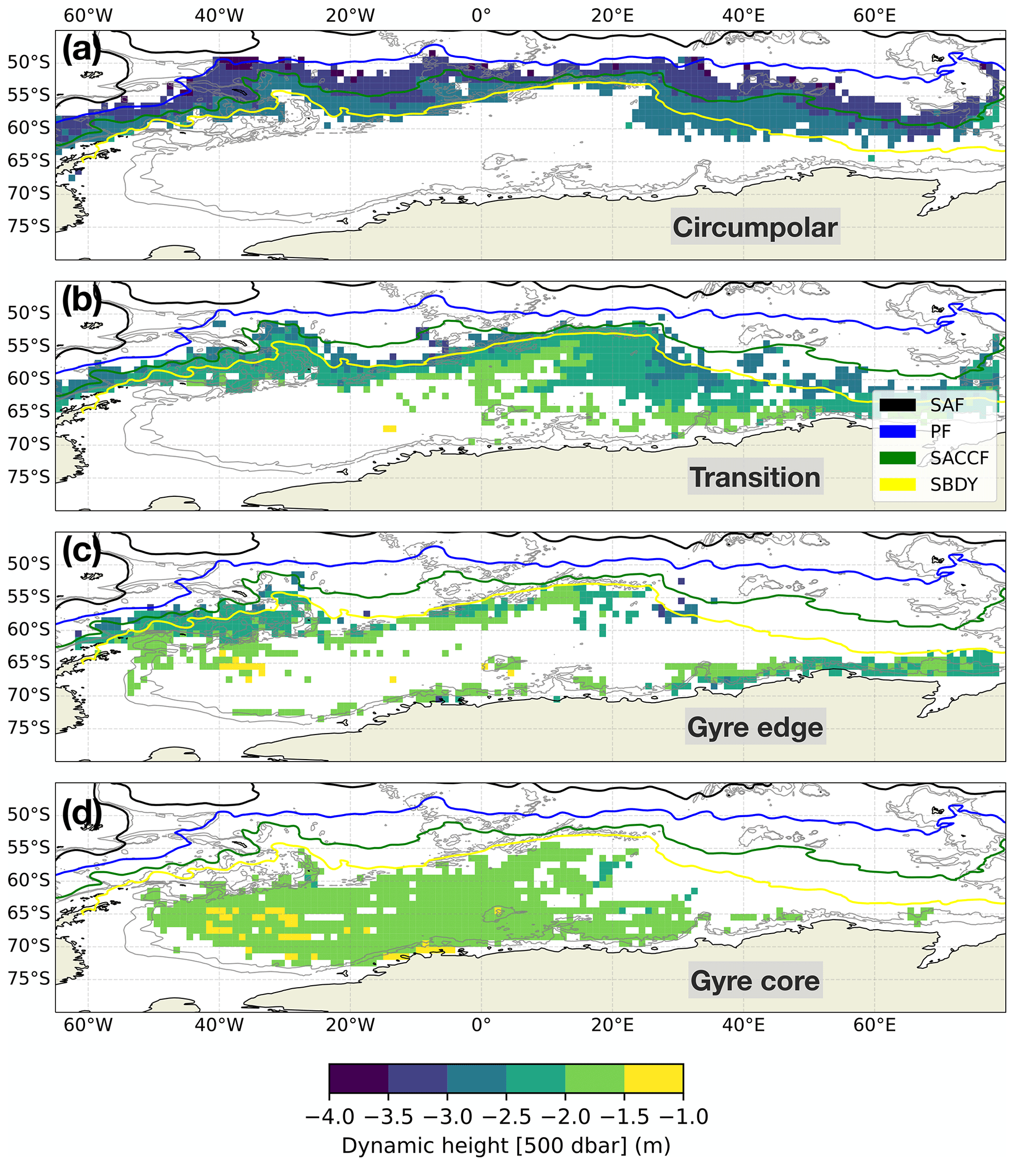
Figure 4Dynamic height of the 500 dbar pressure surface in each of the four classes, binned and averaged over 1∘ latitude–longitude bins. Also shown are several fronts of the ACC from Kim and Orsi (2014), i.e. the Subantarctic Front (SAF), the Polar Front (PF), the southern ACC front (SACCF), and the southern boundary (SBDY). Also shown are contours of constant (thin grey lines), where f is the Coriolis parameter and h is the depth of the water column.
3.2 Signatures of mixing: fuzzy boundaries and the I-metric
As discussed in Sect. 2.2, all GMM-based classification methods, including the ocean-specific PCM approach, are probabilistic. For each profile, the classification algorithm returns probabilities across the classes. PCM assigns each profile to the class with the highest probability, but there is potentially useful information contained in the distribution of probabilities across classes. In order to take advantage of this distribution, we plot the I-metric, which uses the difference between the class with the highest probability and the class with the second-highest probability to quantify the probability that a profile is located at a boundary between classes (Thomas et al., 2021). We can express the I-metric for a single profile as
where P(c=ck)highest is the highest posterior probability that GMM has assigned to the profile, such that the profile has been classified into class ck, and P(c=cl)runner-up is the second-highest posterior probability that GMM has assigned to the profile. If I is small, it indicates that the difference between the probabilities is large; profiles with small I values are not likely to be located near a boundary between classes. If I is large, it indicates that the difference between the probabilities is small; profiles with large I are more likely to be located near a boundary between classes. With oceanographic profile data, the boundaries between classes represent regions of mixing and transformation between profile types associated with changes in one or more water masses that make up the profiles under consideration.
The circumpolar class is characterised by low I-metric values across its entire distribution (median 0.0, third quartile Q3=0.1), except at some locations along its southern edge and in the excursion south of the SBDY between 20 and 40∘ E (Fig. 5a). Note that the low I-metric values along the northern edge of the circumpolar class should be interpreted in the context of the near-Antarctic dataset: there are no profiles north of the circumpolar class in this dataset, so the classification is unambiguous by default. Away from the northern edge, the low I-metric values indicate that the classification is unambiguous in the context of the classification model; the associated profiles are very likely to be in the circumpolar class and unlikely to belong to another class. The transition class features an I-metric distribution with the highest median and third quartile across the four classes (median 0.1, Q3=0.4), consistent with its characterisation as a transition class between the more circumpolar waters and the more gyre-associated waters (Fig. 5b). The highest spatially coherent values, indicating high probability of being at or near a boundary, are found in the southward excursion between 0 and 20∘ E. The gyre edge class also features high I-metric values in some locations (median 0.0, Q3=0.3), particularly in the more western wing just south of the SBDY (Fig. 5c). The profiles near the Antarctic coast tend to have much lower I-metric values. Although it is difficult to state conclusively with profile data alone, the difference in I-metric values between the western wing south of the SBDY and the eastern wing along the Antarctic shelf is consistent with the gyre edge class including both inflowing waters at the eastern edge of the gyre and waters in its northern flank receiving input of shelf waters locally (Fig. 1). Finally, the gyre core class is characterised by low I-metric values (median 0.01, Q3=0.04), indicating an unambiguous “core” profile type, with some mixing and transformation along its edges (Fig. 5d). The slightly higher values between 0 and 20∘E, co-located with the southward excursion of the transition waters, may indicate the signature of the transformation of CDW into WDW in the gyre core.
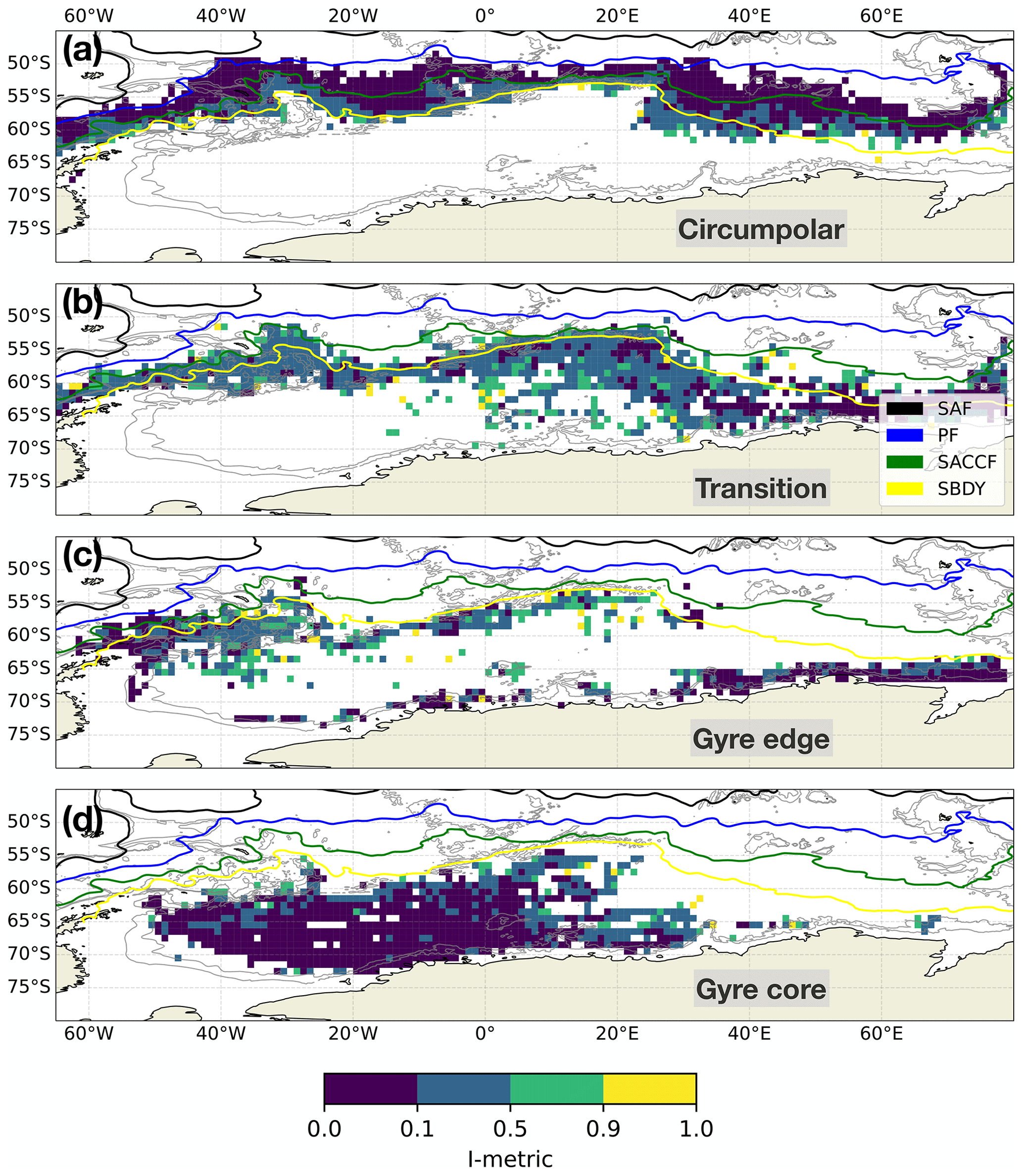
Figure 5Inter-class comparison metric (i.e. the I-metric) binned and averaged over 1∘ latitude–longitude bins. The metric can be interpreted as the probability that the profile is located at a boundary between classes within the Weddell Gyre dataset. Note the uneven spacing of the colour map. The I-metric is defined in Thomas et al. (2021). The fronts and contours are the same as in Fig. 4.
The mixed layer is a layer of roughly uniform density, also described as “weak stratification”, in the upper ocean. It reflects the action of mixing processes that tend to homogenise the near-surface layer of the ocean. Here we examine the distribution of the mixed layer depth, in comparison with the I-metric, to look for potential signatures of regions where mixing has left an imprint on the profile structure. We use the integral depth-scale method described in Thomson and Fine (2003), which estimates the mixed layer depth D as follows:
where zr=1000 m is an arbitrary reference depth and
is the buoyancy frequency, g is the acceleration due to gravity, and ρ0 is a reference density. We calculate using the Gibbs seawater toolbox (McDougall and Barker, 2011).
Broadly speaking, the mixed layer is deeper in the more northern classes and shallower in the gyre core, with some local exceptions (Fig. 6). The circumpolar class features the deepest mixed layers (median 190 m), with especially deep values between 20 and 40∘ E. The transition class, although shallower overall than the circumpolar class (median 140 m), features deep mixed layers along the SBDY, indicating that the imprint of mixing is not uniform across the class. The gyre edge class (median 130 m) also features regions of deeper mixed layers and shallower mixed layers, with deeper mixed layer depths (MLDs) found along the SBDY and the eastern edge along the Antarctic continental shelf. Finally, the gyre core class has the shallowest mixed layers (median 100 m), with some local exceptions along the Antarctic-adjacent contours.
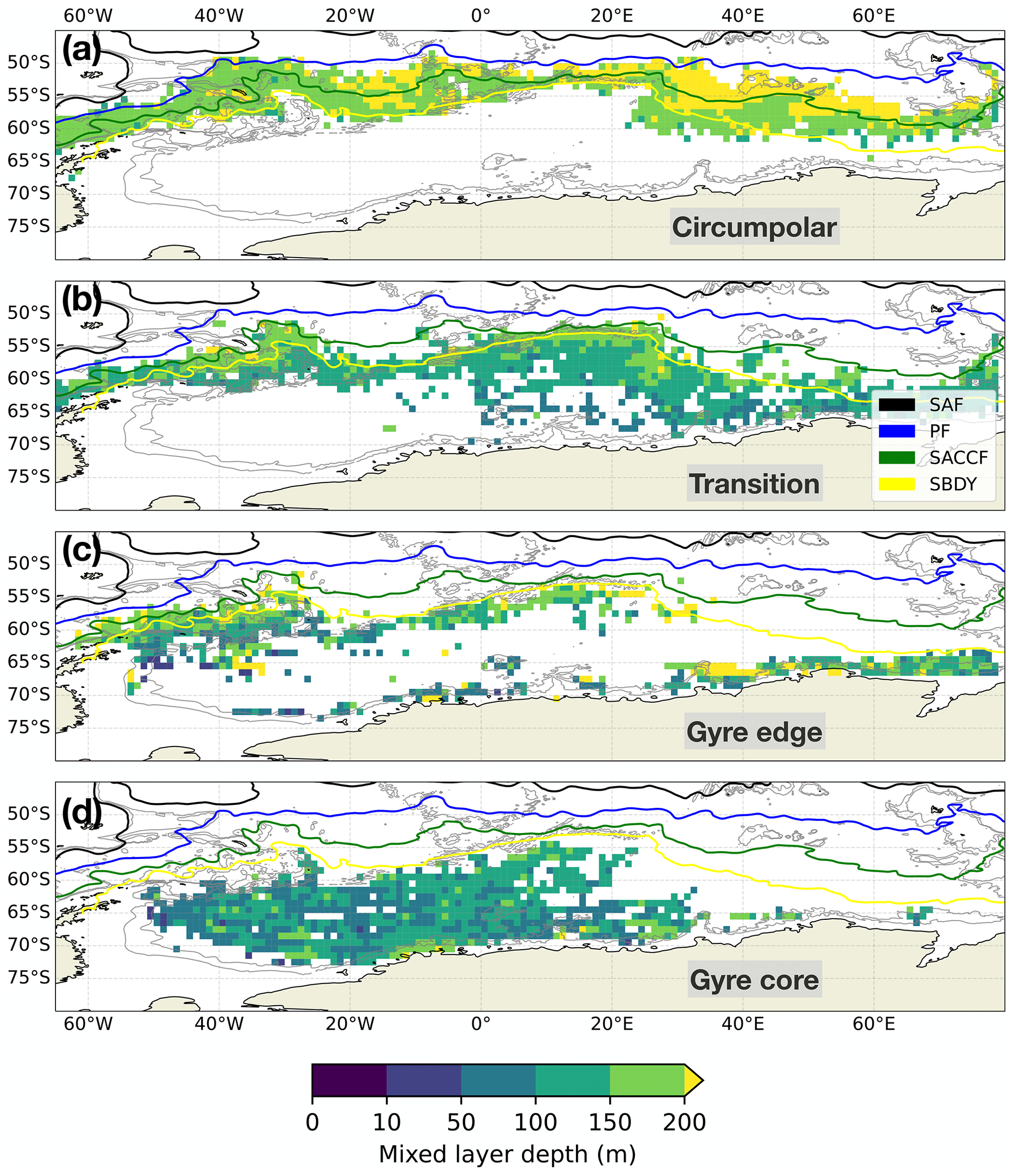
Figure 6Mixed layer depth binned and averaged over 1∘ latitude–longitude bins. The mixed layer is calculated using an integral approach (Thomson and Fine, 2003). The fronts and contours are the same as in Fig. 4.
3.3 Signatures of Winter Water
As discussed in Sect. 3.1, the subsurface temperature minimum seen across the profiles is associated with the WW layer that is formed and renewed seasonally and transported by the near-surface currents. In a broad sense, the depth of the temperature minimum is shallowest at high latitudes and deepest at lower latitudes, although there are localised differences (Fig. 7). In the circumpolar class, the minimum temperature layer is deeper along the northern extent and shallower along its southern extent, and there is a corresponding gradient from warmer minimum values to colder minimum values from north to south (domain-wide median 0.16 ∘C). In the transition class, the temperature minimum is especially deep along the SBDY in the western edge, roughly between the gyre and the Scotia Sea. This is an expected characteristic of the Weddell–Scotia Confluence waters and also of enhanced deep winter convection associated with cold shelf waters (Whitworth et al., 1994). The minimum temperature values there are somewhat warmer than those in the rest of the transition class, especially compared with the cold southward excursion between 0 and 20∘ E. The domain-wide median value of the minimum temperature is colder than that of the circumpolar class (median −0.9 ∘C). The gyre edge and gyre core classes feature extremely cold minimum temperature values (gyre edge median −1.7 ∘C, gyre core median −1.8 ∘C), and the gyre core distribution is colder overall (gyre edge ∘C, gyre core ∘C). Locally in the gyre edge class, as with the transition class, the depth of the temperature minimum is especially deep along the SBDY on the western edge of the domain, although the temperatures are slightly warmer there. The gyre core class features an exceptionally shallow and extremely cold near-surface temperature minimum layer, with a slightly warmer and deeper edge. The processes that establish, renew, and transport the WW layer all leave their imprints on the spatial distributions of the temperature minima and the depths at which those minima are found.
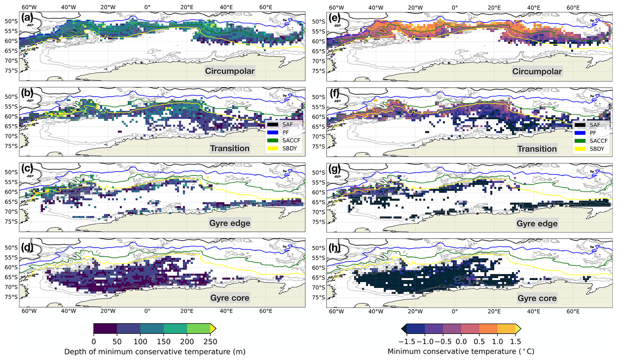
Figure 7Depth of the conservative temperature minimum (a–d) and the value of the conservative temperature minimum (e–h), binned and averaged over 1∘ latitude–longitude bins. The fronts and contours are the same as in Fig. 4.
3.4 Signatures of Circumpolar Deep Water
Most of the profiles in the near-Antarctic dataset feature a subsurface temperature maximum. The temperature maximum represents the core of CDW; we can use this layer to track the core of the CDW as it is transported from the circumpolar region to the Weddell Gyre (Reeve et al., 2016, 2019). In the circumpolar class, we see the core of the CDW deepen and cool along the length of the ACC, with especially deep and cold values in the southward excursion south of the SBDY between 20 and 40∘ E (Fig. 8). In the transition class, we see a gradient in the CDW-associated temperature maximum, getting colder along the southward excursion, where it meets up with the western edge of the gyre core and the WDW. The gyre edge class features particularly deep and cold temperature maxima (median ∘C, median depth 500 m), with the deepest Tmax depths of all the classes. By contrast, the gyre core class is characterised by somewhat shallower temperature maxima (median ∘C, median depth 260 m). The fact that the gyre edge class exhibits a much deeper temperature maximum than the gyre core class is a key difference between the two, possibly highlighting that the processes setting the depth of Tmax may be different between them. The gyre edge class may be more associated with the circulation of WSDW around the edge of the gyre and the doming down of isopycnals along its boundary (Fig. 1). Notably, there is a clear difference in the depth of the temperature maximum along the gyre core in the east–west direction, with a deeper layer in the west and a shallower layer in the east (Fig. 8d). This is consistent with CDW intrusion into the eastern edge of the gyre class.
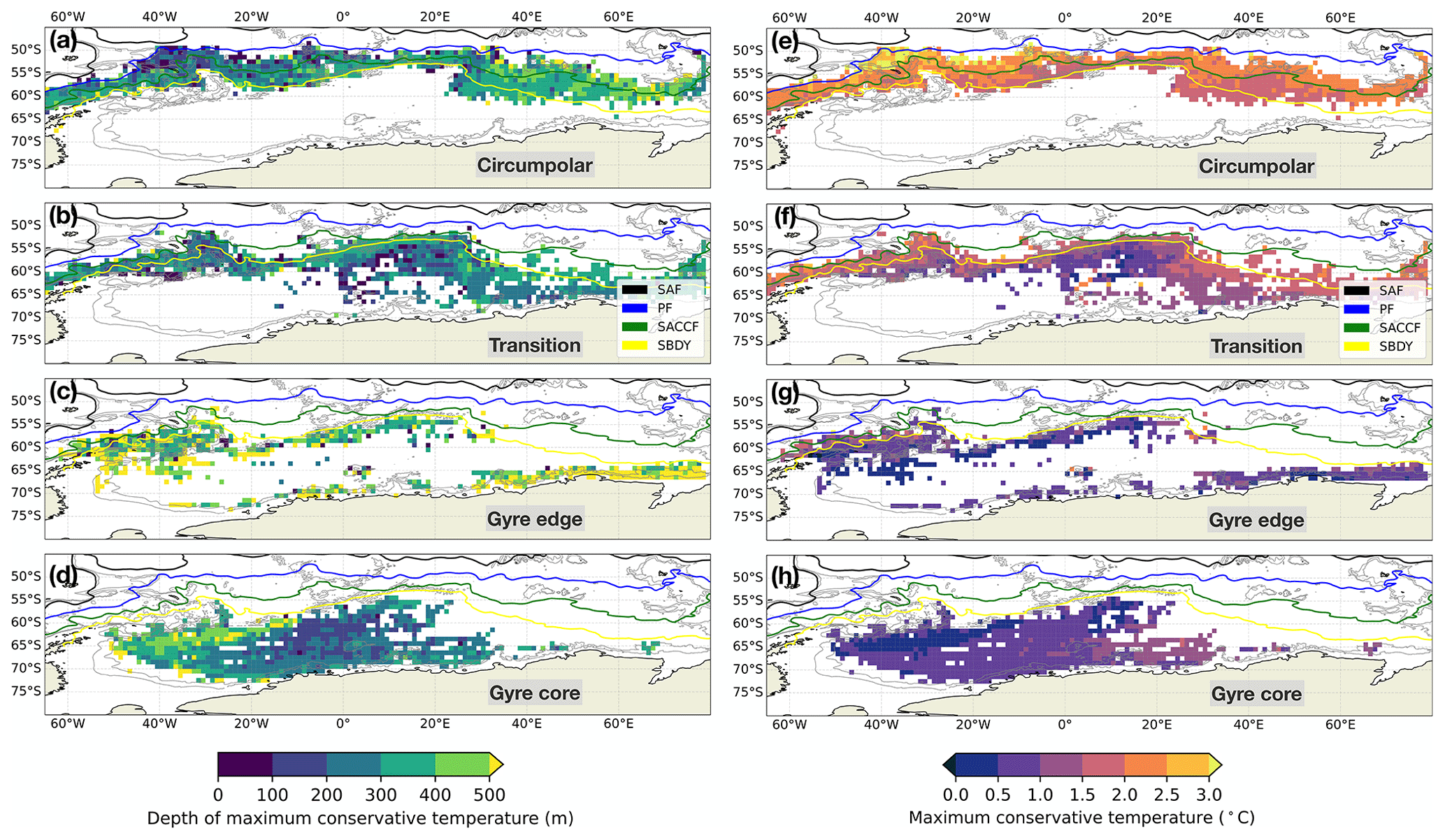
Figure 8The depth of the maximum conservative temperature (a–d) and the value of the maximum conservative temperature (e–h), binned and averaged over 1∘ latitude–longitude bins. The fronts and contours are the same as in Fig. 4.
3.5 Signatures of mixing between Circumpolar Deep Water and Winter Water
All four classes are characterised by a proportion of relatively salty, dense, and warm water and a proportion of fresher, colder, and lighter water (Fig. 9). The salty, dense, warm waters have properties consistent with CDW and occupy the right-hand side of the θ–S plots in Fig. 9. The fresh, cold, light waters have properties consistent with a layer of temperature minimum WW, sitting along the bottom of the θ–S plots. The WW becomes increasingly salty as we consider the classes in order of proximity to the gyre core: i.e. circumpolar, transition, edge, core. Broadly speaking, there are two possible causes for this: (1) the effect of brine rejection associated with sea ice formation leads to saltier WW varieties, and (2) the core of CDW, which is characterised by a subsurface temperature maximum, is shallower in the gyre classes due to upwelling. Both of these signatures lead to enhanced vertical mixing between CDW and the overlying WW.
Although all four classes feature CDW, WW, and surface water (SW), there is a key difference between the circumpolar waters and those of the transition class: compared with the circumpolar class, the transition class is more affected by brine rejection from sea ice formation and the mixing associated with this brine rejection. In particular, there is a range of θ–S space that is unoccupied in the circumpolar class but more populated in the other classes, notably the transition class (Fig. 9, grey oval). We hypothesise that this region in θ–S space is associated with mixing between CDW and WW; the circumpolar class is less affected by this mixing, whereas the transition class is more influenced by this mixing. Furthermore, the two gyre classes feature strong mixing between CDW and WW, enabled in part by upwelling in the cyclonic gyre. The “mixing line” between CDW and WW is especially compact and straight in the gyre core class, which is consistent with CDW and WW being physically closest to one another there.
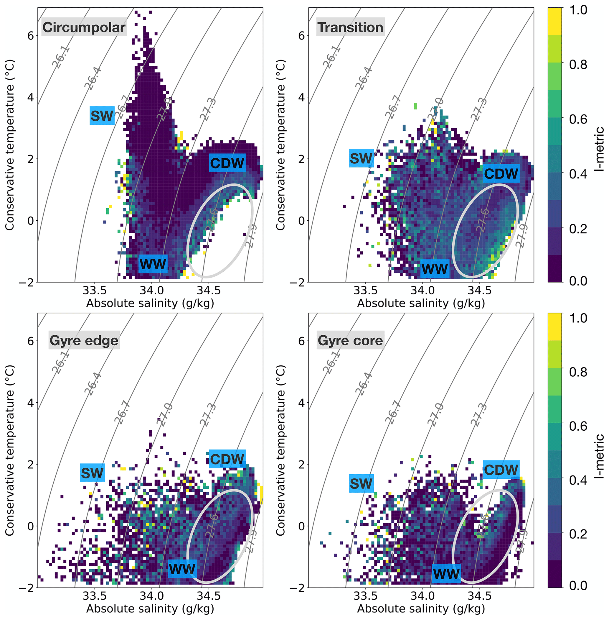
Figure 9Temperature–salinity diagrams for the four classes. The shading indicates the mean I-metric value for each bin (0.1 ∘C, 0.025 g kg−1). Since each profile has a single I-metric value, the approach used here averages all profiles that pass through any given bin. The result is a relative indication of the core class properties versus the more peripheral ones. The solid lines are potential density contours (σ0). The grey oval indicates a potential signature of mixing between the Winter Water and deeper water. Also shown are the approximate locations of the surface water (SW), Circumpolar Deep Water (CDW), and Winter Water (WW).
Across all four classes, the seasonal cycle is characterised by a weakening of the near-surface temperature stratification in austral winter and spring (JJA and SON), followed by restratification in the austral summer and autumn (DJF and MAM) as the SW warms (Fig. 10). The layer of WW remains trapped under the warmed, restratified near-surface waters, decaying somewhat by mixing until it is ventilated again during the following winter and spring. The warmer waters of the CDW that sit below the WW remain steady throughout the year, as they are more isolated from the processes associated with the seasonal cycle. In terms of salinity, all four classes feature year-long stability in terms of fresher waters overlying saltier waters, although there is a clear near-surface seasonal cycle (not shown).
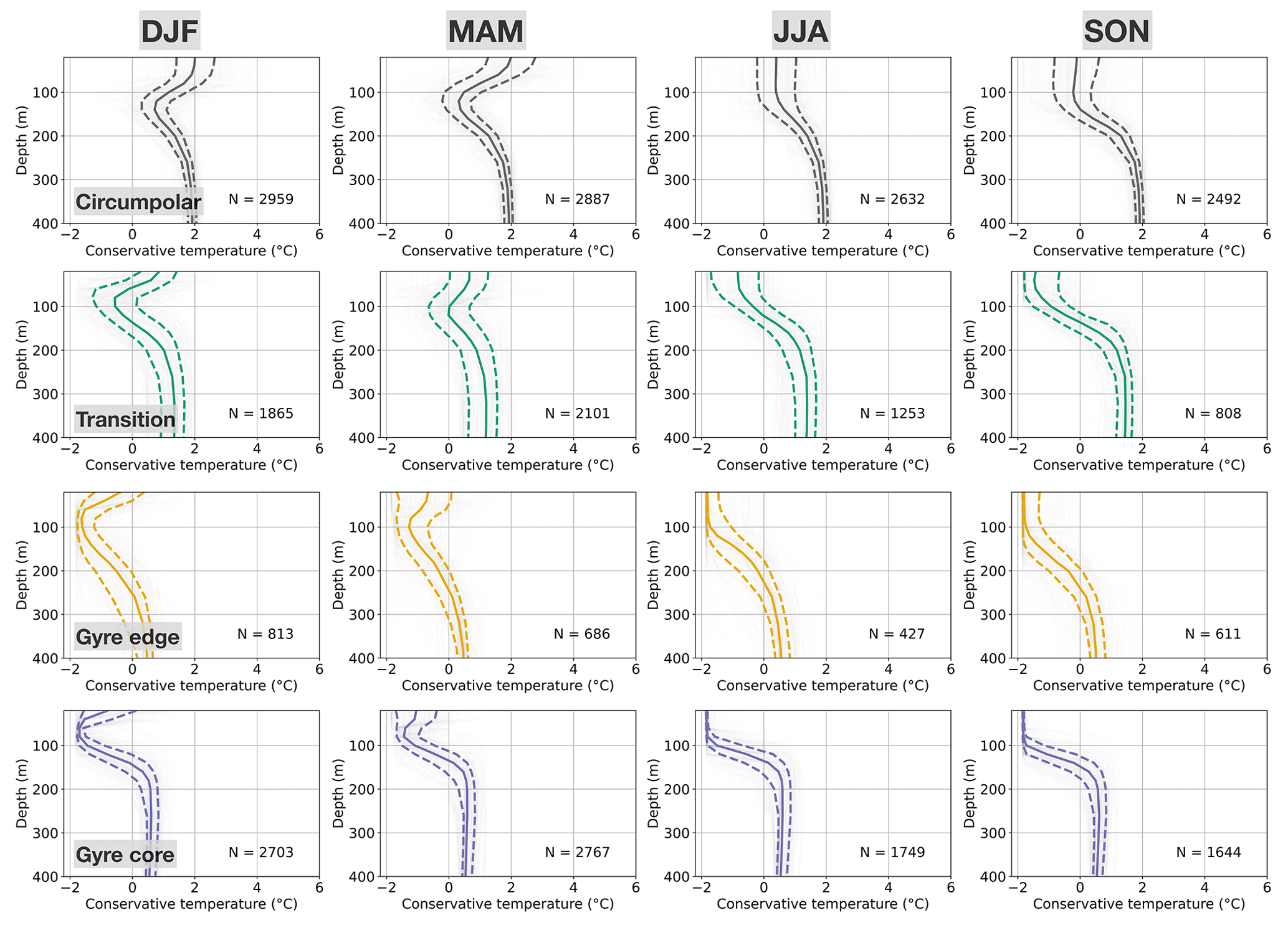
Figure 10Distribution of the conservative temperature of the four classes, split by season. Each panel features a random selection of 400 profiles (thin grey lines), the 25th percentile (dashed line, left), the median (solid line), the 75th percentile (dashed line, right), and the number of profiles N in each class and season.
The circumpolar and transition classes are characterised by the formation of WW in winter and spring, with its rapid erosion in summer and autumn (Fig. 11, top two rows). The circumpolar class features a strong seasonal cycle in SW, warming and cooling largely by heat transfer with the atmosphere. The transition class also displays a stronger seasonal cycle in SW. In contrast, in the gyre edge and gyre core classes, the WW is present year-round, and mixing between WW and CDW, as inferred by the density of profiles along the “mixing line” between the two water masses, appears to be weakest in winter and stronger throughout the rest of the year.
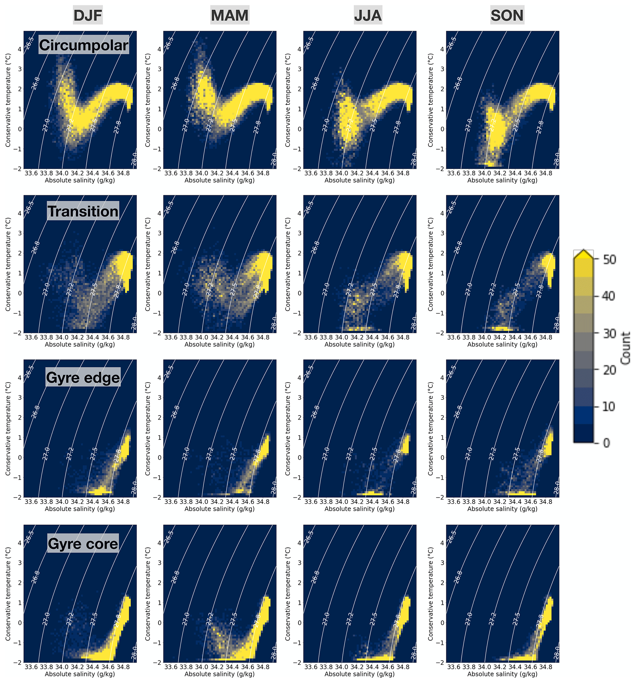
Figure 11θ–S diagrams grouped by class and season. The colour indicates the number of profiles passing through each θ–S bin (width 0.1 ∘C, 0.025 g kg−1), and the solid lines are potential density contours.
We also examined the spatial structure of the seasonal cycle, specifically in the mixed layer depth, the depth of the temperature minimum, and the depth of the temperature maximum. The seasonal cycle displays little spatial variation, mostly highlighting property gradients that are already detectable in the climatological average. For instance, the conservative temperature minimum in the transition class is especially deep in the western part of the domain during the summer and autumn, particularly along the SBDY (Fig. 12), as seen in the climatology (Fig. 7). The east–west contrast in the depth of the temperature minimum becomes less apparent in the winter and spring as surface cooling refreshes the Winter Water layer. The region of CDW intrusion is less apparent in the winter and spring due to spatial sampling biases over these seasons.
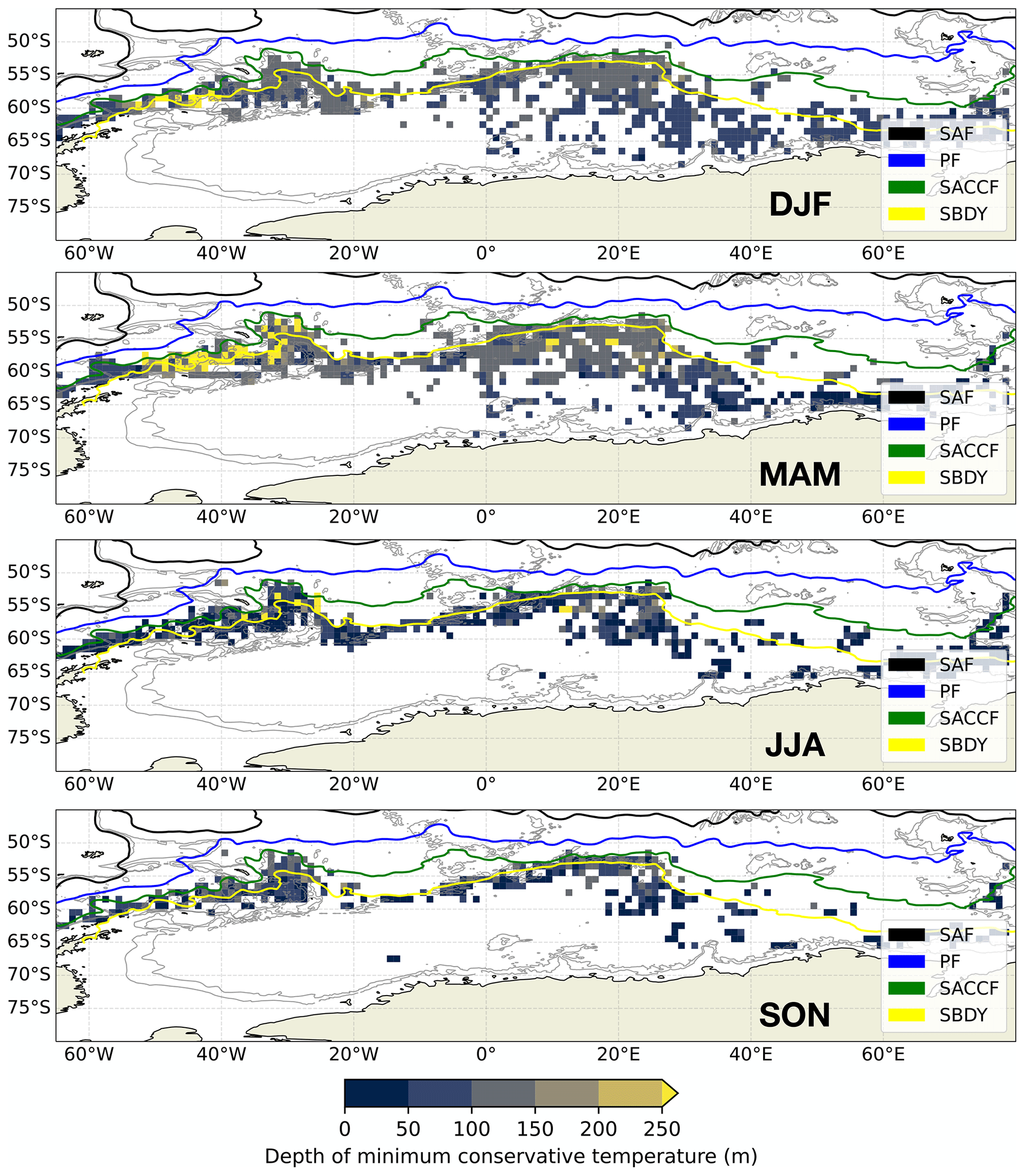
Figure 12Depth of the minimum conservative temperature of profiles that belong to the transition class, averaged over 1∘ latitude–longitude bins and separated by season.
3.6 Physical context: surface stress, upwelling, and sea ice
Here we discuss two physical fields that are relevant to our interpretation of the classes: surface-stress-driven (Ekman) upwelling and freshwater flux from brine rejection. In the Southern Ocean, surface stress is set by near-surface winds and modulated by the presence of sea ice through both ice coverage of the ocean surface and stress associated with sea ice drift (Dotto et al., 2018). The Ekman upwelling velocity at the base of the Ekman layer is
where ρ0 is the reference density, τ is the surface stress from ERA-5 reanalysis following Dotto et al. (2018), and f is the Coriolis parameter. We find climatological upwelling of various intensities along the SBDY, which is co-located with the edge of the circumpolar class, the core of the transition class, and the northern extent of the gyre edge class (Fig. 13a). There is also weaker upwelling throughout the gyre core, which is consistent with its cyclonic circulation and the associated upwelling of CDW throughout. We find downwelling in the western edge of the domain near the Filchner–Ronne Ice Shelf and patches of strong downwelling along the rest of the Antarctic coast (Fig. 1). This near-coastal downwelling seemingly affects the southern extent of the gyre edge class as well as the edges of the gyre core class.
In order to further investigate our hypothesis that the transition class is more influenced by brine rejection from sea ice formation compared with the circumpolar class, we examine an estimate of salt input associated with winter sea ice formation from a regional state estimate (Mazloff et al., 2010). We find that in the western part of the domain, the strongest brine rejection largely coincides with the position of the SBDY, which again is co-located with the core of the transition class (Fig. 13b). This positioning is consistent with the hypothesis that brine rejection is able to affect the transition class more than the circumpolar class, which is found mostly north of the SBDY. In the eastern part of the domain, the salt input associated with sea ice mostly aligns with the SACCF, but this is somewhat downstream of our main analysis region near the Weddell Gyre. These results are compatible with those of Haumann et al. (2016), who find both local freezing and transport to be important for setting the freshwater input south of the region of maximum sea ice extent (their Fig. 4).
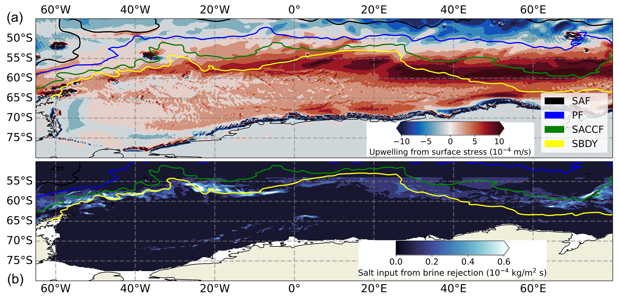
Figure 13(a) Estimated upwelling (10−4 m s−1) from surface stress, including the effects of wind stress, sea ice coverage, and sea ice drift, following Dotto et al. (2018). The sea ice concentration is from the Climate Data Record v4, and sea ice drift is from Polar Pathfinder. (b) Approximate position of the wintertime sea ice freezing line, as indicated by the salt input from brine rejection during sea ice formation (negative freshwater input, shown in units of 10−4 kg m−2 s−1). Values below 10−5 kg m−2 s−1 have been masked out (i.e. set to zero). Data from SOSE averaged over JAS during the period 2005–2010 (Mazloff et al., 2010). The fronts are the same as in Fig. 4 from Kim and Orsi (2014).
The Weddell Gyre region controls the properties of some of the densest waters on the planet, with associated effects on the overturning circulation and on the air–sea partitioning of heat and carbon (Vernet et al., 2019). Because of these unique properties, the structure and variability of the Weddell Gyre are relevant to how it functions as part of the global ocean and climate system. In this work, we applied a profile classification model (PCM), which is a type of unsupervised machine learning, to a temperature and salinity profile dataset covering the Atlantic sector and part of the Indian sector of the Southern Ocean. Our objective was to use the PCM as a “discovery tool” to identify thermohaline structures in the Weddell Gyre region and to examine their seasonal variability. Our application of PCM identified four coherent “profile types” that can be described as follows: (1) a circumpolar class that largely sits north of the SBDY, (2) a transition class between the circumpolar region and the gyre region, (3) a gyre edge class with northern and southern regions, and (4) a gyre core class. The four classes are reasonably interpretable and geographically distinct from one another, with some overlap as expected when using a probabilistic classification scheme such as PCM on a highly correlated dataset.
PCM identifies some key features of the Weddell Gyre region and its circulation, refining our current understanding of this complex structure (Vernet et al., 2019). Some specific refinements to our understanding include the following.
-
The intermediate region between the ACC and the Weddell Gyre is more complex than a single confluence region between them. There is a transition class and a distinct gyre edge class that bears some similarities to waters that are much closer to Antarctica (e.g. Fig. 4b, c).
-
This intermediate region extends much further east than previously thought for the Weddell–Scotia Confluence (Patterson and Sievers, 1980; Vernet et al., 2019).
-
The intrusion of CDW into the gyre occurs over quite a broad region (20–40∘ E), as evidenced by circumpolar-class waters intruding south of SBDY (e.g. Fig. 4b).
-
The transition waters are meridionally much broader east of the Greenwich Meridian than the west, suggesting the role of topography (i.e. the South Scotia Ridge) in constraining the interaction of water masses between the ACC and the gyre, consistent with Patmore et al. (2019) (e.g. Fig. 4b).
-
The gyre edge class indicates some level of similarity between waters at the northern and southern ends of the gyre, where waters from Antarctic shelves can be injected directly into mid-depths (i.e. WSC in the north or the descent of dense shelf waters into CDW layers in the south) (e.g. Fig. 4c).
-
The gyre core bifurcates and is strongly influenced by underlying topography around 10–20∘ E, which is a refinement of our understanding of this two-cell structure (e.g. Fig. 4d).
-
The gyre core seems to follow the continental slope very closely in the south – there is a sharp transition here (e.g. Fig. 4d).
In addition, PCM reveals aspects of the spatial distribution of mixing between WW and CDW. It also characterises the seasonal cycle of the four classes, highlighting the formation, extent, and destruction of WW throughout the gyre and its surroundings via mixing with the underlying CDW (Sect. 3.5). The spatial and temporal structure of when and where WW and CDW most readily mix, with sea ice as a key determinant, had not been identified before. We discuss this further in the next subsection.
4.1 Influence of sea ice processes on class structures
Sea ice growth, brine rejection, and vertical mixing are closely related in the polar regions (Gordon and Huber, 1990; Martinson, 1990). A key result from this study is the marked difference between waters where WW and CDW more readily mix with each other (i.e. the transition and gyre classes) and the more northern class wherein the WW and CDW are more isolated from one another (i.e. the circumpolar class); this is especially apparent when viewed in θ–S space (Fig. 11). In particular, we hypothesise that the structure of the transition class is affected by salt input from sea ice processes (e.g. brine rejection) and the associated mixing, whereas the circumpolar class is not especially affected by this process. Local freezing and sea ice formation tend to add salt to the regions occupied by the transition class in a climatological sense, which would weaken the stratification and thereby encourage mixing between WW and CDW (Haumann et al., 2016). This process is most relevant in JJA and SON, when sea ice reaches its maximum extent and is most aligned with the SBDY in the western Weddell Gyre (Fig. 13). Although this same region is also affected by freshwater flux due to melting and sea ice export, which would have a stabilising effect on the water column during some parts of the year, this would not necessarily eliminate the effect of wintertime salt flux from brine rejection and the relative increase in mixing.
As a further contributing factor, it may be that the weak stratification of the transition class is related to the spillage and subsequent eastward advection of relatively dense and weakly stratified shelf waters from the tip of the Antarctic Peninsula. Those waters have had their stratification reduced by sea ice production and brine rejection on the continental shelves of the western Weddell Sea. Quantifying the relative effect of local brine rejection and advection on the transition and circumpolar classes may be a fruitful avenue for future observational and numerical studies.
4.2 Influences of bathymetric and shelf processes on class structures
Using PCM, the boundaries between classes are probabilistic and somewhat “fuzzy”. That being said, many of the approximate class boundaries roughly coincide with Southern Ocean fronts, the positions of which are strongly linked to bathymetry. As an example, the boundary of the circumpolar class approximately aligns with the SBDY, which is constrained by the South Scotia Ridge. This correspondence is consistent with studies that have shown the importance of bathymetry, including ridge geometry, in determining the stratification, circulation, and extent of the Weddell Gyre (Patmore et al., 2019; Wilson et al., 2022).
Processes on the continental shelves also affect the structure of the classes. For example, ventilation may affect the structure of the southern wing of the gyre edge class, as it is largely distributed along the Antarctic continental shelf. The transition class may be affected by ventilation by low-salinity shelf waters along the eastern Weddell Gyre. These shelf waters are not dense enough to support AABW formation; instead, they cascade down along the continental slope and ventilate the CDW (Thompson et al., 2018).
4.3 A novel characterisation of the Weddell–Scotia Confluence waters
The northern and southern branches of the gyre edge class show similarities in structure that justify their grouping together by the PCM (i.e. increasing the number of classes does not separate out these branches). However, there are discernible differences between the two branches (Fig. 14). The northern branch is characterised by warmer and slightly fresher surface waters and has weaker stratification below 300 m. Although we must be cautious in interpreting any possible dynamical relationship between the branches, these observations are consistent with the flow of surface waters along the ASF, mixing with the fresh shelf waters and warming as they turn northwards to join the WSDW.
The location and weak stratification of the northern branch align with the properties of the Weddell–Scotia Confluence waters, which are characterised by weak mid-depth stratification and are found close to the South Scotia Ridge (Patterson and Sievers, 1980). Initially attributed to topographic mixing, this reduced stratification is now understood to result from the spillover of shelf water from the Antarctic Peninsula tip and its eastward spread (Whitworth et al., 1994). While each class or profile type in a PCM is shaped by multiple processes, the spatial coincidence of the northern branch of the gyre edge class with the Weddell–Scotia Confluence (Fig. 5) is noteworthy. Along the SBDY, I-metric values of the gyre edge class profiles tend to increase from west to east, indicating some mixing between profile types. The PCM does not distinguish causes or dynamical connections, but the coherence of the northern branch along the length of most of the SBDY suggests that WSC signatures may be detectable further west than previously thought. This alternative characterisation of the WSC is a key result of this study.
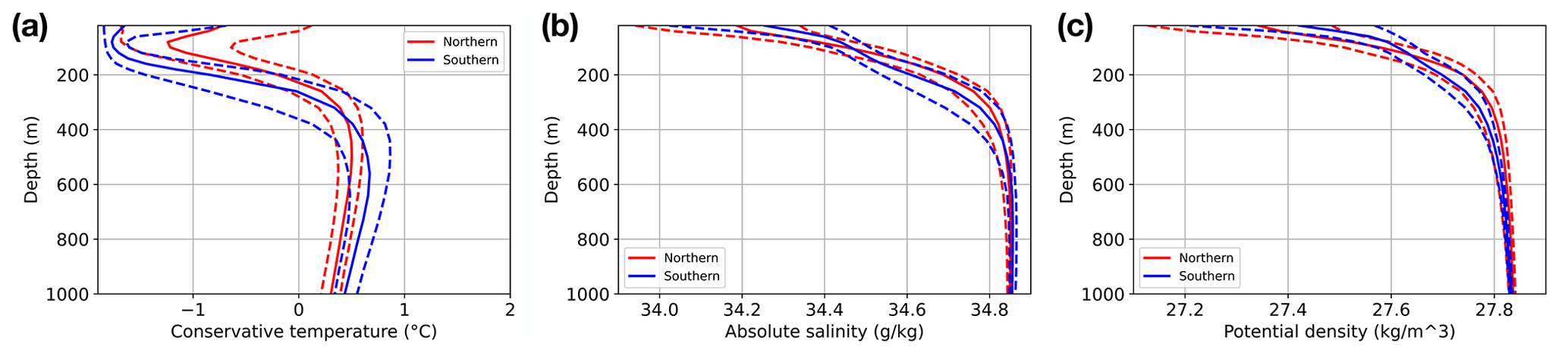
Figure 14Comparison of the conservative temperature (a), absolute salinity (b), and potential density (c) of the northern (red lines) and southern (blue lines) extents of the gyre edge class. The solid lines represent median values, and the dashed lines represent the 25th and 75th percentiles of the distributions at each depth level.
4.4 The case for regional, application-specific profile classification models
As with many classification problems, there is a balance to strike between the interpretability of the PCM and its accuracy, i.e. its ability to represent the full underlying covariance as captured by the available data. The ideal balance depends on the objective of the study; if interpretability is the main objective, then one can opt for fewer classes, with less overlap between them. If accuracy is the main objective, then one can opt for more classes, with more overlap between them. Typically, as overlap increases, the ease of interpretation decreases. That being said, even in the simplest case with as few as two classes, each “profile type” will bear the integrated signatures of many different processes (e.g. mixing between water masses, air–sea interactions), so they must be interpreted in a way that considers this integration. Some statistical guidance is available for helping with our choice of the number of classes, but this guidance often returns a range of allowed numbers of classes as opposed to a single objective value (Fig. A3). It is sometimes instructive to compare the structures of PCMs with different numbers of classes, much as one might compare different levels of complexity in a hierarchy of numerical models (Held, 2005). One can learn about the structure of the system by observing what changes as one adds or removes sources of complexity, in this case by adding or removing classes.
The structure of the PCM also depends on its temporal and spatial domain. The goal of identifying a single global, unified PCM is likely an impractical one, as the “noise” in a global PCM might well be a meaningful “signal” in a more regional PCM. This is analogous to identifying fronts in the Southern Ocean; the way we treat structures and the boundaries between them benefits from a more region-specific, application-specific approach for similar reasons – one application's “signal” is another application's “noise” (Chapman et al., 2020; Thomas et al., 2021). As with many atmospheric and oceanographic problems, filtering, signal processing, and the context of the variability are all routinely used to highlight certain features and aid understanding. The flexibility of PCMs is one of their strengths; they can be focused on specific regions, variables, and types of variability depending on the objective of the application at hand.
That said, the four-class model derived here could be compared to the Southern Ocean temperature-only PCM presented in Jones et al. (2019). In that study, there are only two classes south of the PF, i.e. a near-Antarctic class located broadly in the gyres and along the slope current and a more circumpolar class that runs just south of the PF. As we found in the Weddell Gyre PCM, the profile types found south of the PF are characterised by salt stratification. Although one should be careful not to overinterpret, the circumpolar class in the temperature-only Southern Ocean PCM is roughly analogous to the circumpolar class found here in the Weddell Gyre-specific PCM. The Weddell Gyre PCM is able to distinguish additional structure because it (1) includes salinity as a variable and (2) is focused on a regional set of profiles.
4.5 Identifying the underlying covariance structure
The actual grouping or classification of the profile data happens in an abstract principal component (PC) space. In PC space, the covariance structure of the dataset, in terms of both its climatology and the seasonal cycle, is represented by a “circumpolar wing” and a “gyre wing”, separated by a transition bridge between the two. This is similar to what one sees using t-distributed stochastic neighbour embedding (t-SNE), which is a nonlinear mapping technique that can be useful for visualising high-dimensional data (van der Maaten and Hinton, 2008). This approach gives us an alternative way to understand the underlying covariance structure in the Weddell Gyre region, which is ultimately what we are trying to estimate using PCM. The t-SNE method takes a set of high-dimensional points and maps them onto two dimensions, ideally “keeping close neighbours close and distant neighbours distant” (Kobak and Berens, 2019). The dominant free parameter of t-SNE is the perplexity, which, very roughly speaking, indicates the level of “attraction” present between nearby points during the fitting process. Low values indicate weak attraction, whereas high values indicate strong attraction. We fit t-SNE using four different perplexity values using an optimised, automatic learning rate (Belkina et al., 2019). Because t-SNE is stochastic in the sense that different initialisations can produce somewhat different results, we ran the fitting process multiple times for each value of perplexity, finding that the large-scale structure in t-SNE space is robust, with only smaller-scale variations.
The structure in t-SNE space consists of a circumpolar wing, a transition bridge, and a gyre wing with (1) a gyre edge region, which is connected to the transition bridge, and (2) a gyre core region, which is somewhat more separated from the transition bridge (Fig. 15). The separation between the circumpolar profiles and the gyre core profiles is consistent with their separation in physical and property space as well. For example, it is unlikely that a circumpolar profile could transform directly into a gyre core profile without first passing through the transition class. Generally speaking, PCA by definition does not capture nonlinear structures, whereas a method like t-SNE does. One example of such a nonlinear feature is how the transition class is split into multiple components, for instance at the tip of the gyre core class, wherein we find a small group of mixed transition and gyre edge points. Further investigation indicates that this small group consists of points from the high-latitude, far eastern portion of the domain, south of approximately 65∘ S and between roughly 40 and 70∘ E. This represents an area of overlap between the transition class and the southern extents of the gyre edge class (Fig. 15). In this case, t-SNE highlights the difference between the lower-latitude transition bridge and the higher-latitude, far eastern transition–core and transition–circumpolar overlaps, which is not apparent in PC space (Fig. A4).
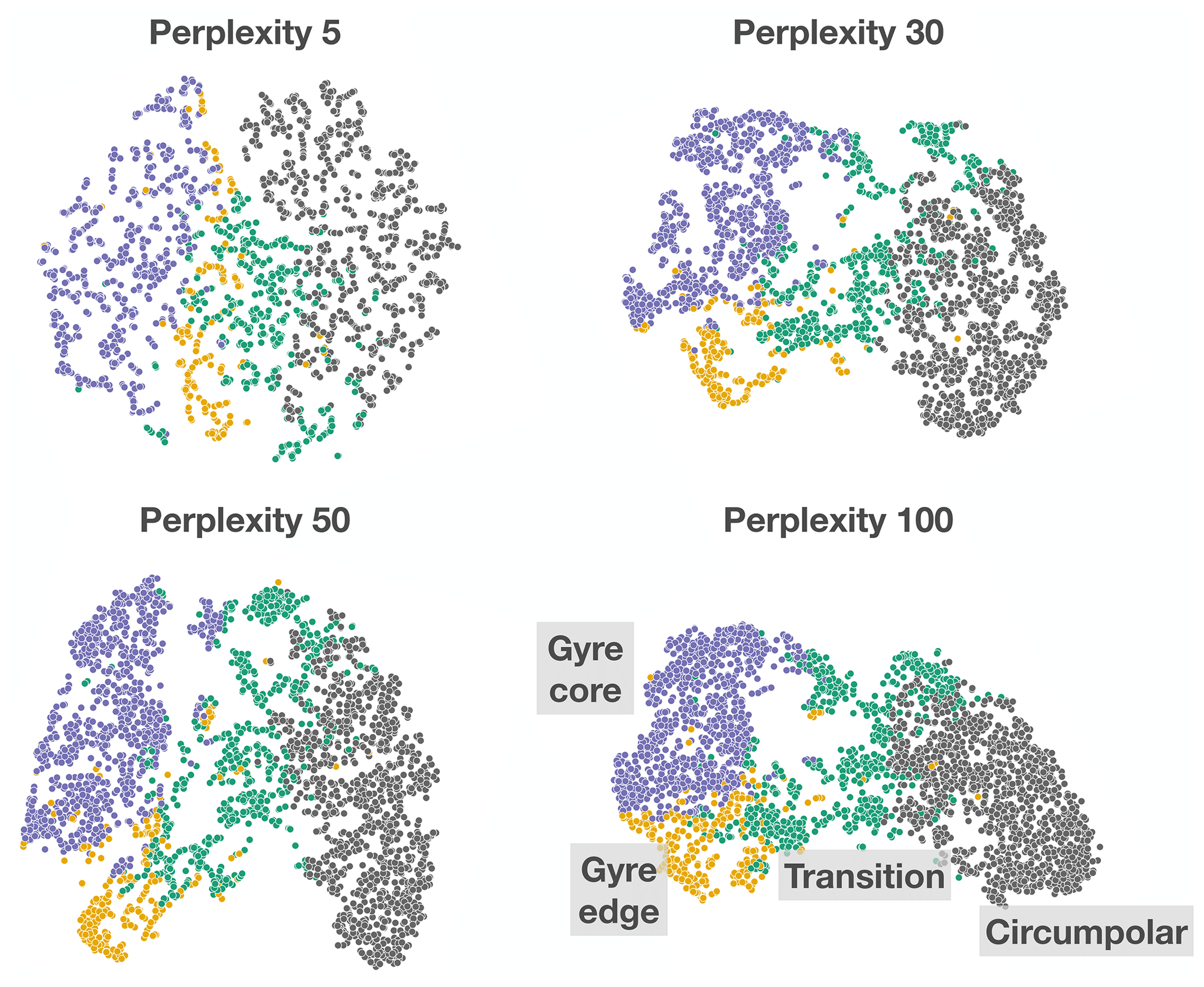
Figure 15Visualisation of six-dimensional principal component space, transformed into a 2D space using t-SNE (Maaten and Hinton, 2008). The colours indicate the four classes into which the profiles have been sorted. Roughly speaking, the perplexity indicates the level of mutual “attraction” between nearby points during the fitting process. The axes are arbitrary dimensions and should not be interpreted quantitatively; they are for visualisation purposes only.
In abstract t-SNE space, one might consider the probability of a transition from the circumpolar wing to the gyre wing via the transition class. This framework makes the most sense in a more barotropic conceptual model of the Weddell Gyre, which may be defensible in the upper O(1000 m) of the region, since the circulation in this layer is more likely to be equivalent barotropic compared with the entire water column (Killworth, 1992; Marshall, 1995; Krupitsky et al., 1996). The presence of baroclinicity implies the presence of shear, which likely only happens in specific locations (e.g. associated with bathymetric features). Another way to frame this would be to ask the following: what transformations would be necessary to convert a profile from the circumpolar wing to the gyre wing via the transition bridge? Examining the profile types, we can speculate that such a transformation would involve cooling throughout the water column, a shoaling and weak salinification of the WW layer, a deepening of the core of the CDW, and an overall weakening of the subsurface stratification.
4.6 The limitations of spatial and temporal bias
The set of profiles used in this study are not distributed uniformly in space or season. Some locations are overrepresented, for instance along repeat hydrographic sections (e.g., A12, A13.5). In order to minimise the effect of this spatial bias on the PCM, we selected training datasets that are approximately uniform in terms of areal coverage. We also carried out a sensitivity test wherein the training datasets were generated randomly with no guarantee of uniformity, and the results were broadly unchanged (not shown). In terms of temporal coverage, the austral winter and spring months are somewhat underrepresented relative to the rest of the year (Fig. 2b), which may bias the PCM towards summer and spring structures. However, since the total number of profiles in any given class and season is fairly small, we decided to use all available data instead of further sub-selecting for the training dataset. Although this does introduce what we expect to be a small bias in the PCM, we weighed this against the size of our dataset and decided to proceed with more profiles rather than fewer. The profile dataset is also non-uniform by year; this will also introduce some biases into our PCM. Because we are basically using the PCM to build up a climatological and seasonal mean picture of the structure of the Weddell Gyre, we do not think that our results would change drastically using uniform sampling by year. Nevertheless, this bias highlights the need for continued profile-based monitoring of the Weddell Gyre and the surrounding areas so that we may develop a more complete understanding of the seasonal cycle as well as interannual to decadal variability.
Through the processes of dense water formation and upwelling that occur in and around the Weddell Gyre, this unique region connects the atmosphere, surface ocean, and the deep ocean. Its structure and variability are relevant to how it functions as part of the global ocean and climate system. In this work, we used a profile classification model (PCM), a type of unsupervised classification built on Gaussian mixture modelling (GMM), as a tool for characterising temperature and salinity profile data in the Weddell Gyre region. The PCM highlights both expected and underappreciated structures, helping to generate new hypotheses for further investigation. Specifically, the Weddell Gyre PCM identified four different “profile types”, namely (1) a circumpolar class, (2) a transition class between the circumpolar profiles and the gyre profiles, (3) a class of profile on the edge of the gyre, and (4) a class of profiles in the core of the gyre. The vertical structure and geographic distribution of the classes feature signatures of CDW inflow across the eastern boundary of the Weddell Gyre, the presence of the Weddell–Scotia Confluence, and the spatial distribution of mixing between the WW and CDW. The seasonal cycle of the class structure highlights the formation, extent, and mixing of WW throughout the gyre and its surroundings. We put forward the hypothesis that the transition class is more affected by mixing encouraged by brine rejection from sea ice formation compared with the circumpolar class, as suggested by the spatial overlap between the northern edge of winter sea ice production and the transition class. Unsupervised classification approaches such as PCM can complement existing expertise-driven analysis, which has been and will remain useful well into the future. Future studies that examine alternative classification strategies (e.g. agglomerative clustering) would be a welcome addition to the literature.
In this Appendix, we describe some details of the PCA and PCM approaches used in this work. In Sect. A1, we discuss dimension reduction using the principal component approach. In Sect. A2, we describe the procedure used to select the number of classes. Finally, in Sect. A3, we provide some mathematical details for GMM, which is the underlying unsupervised classification approach used in our PCM.
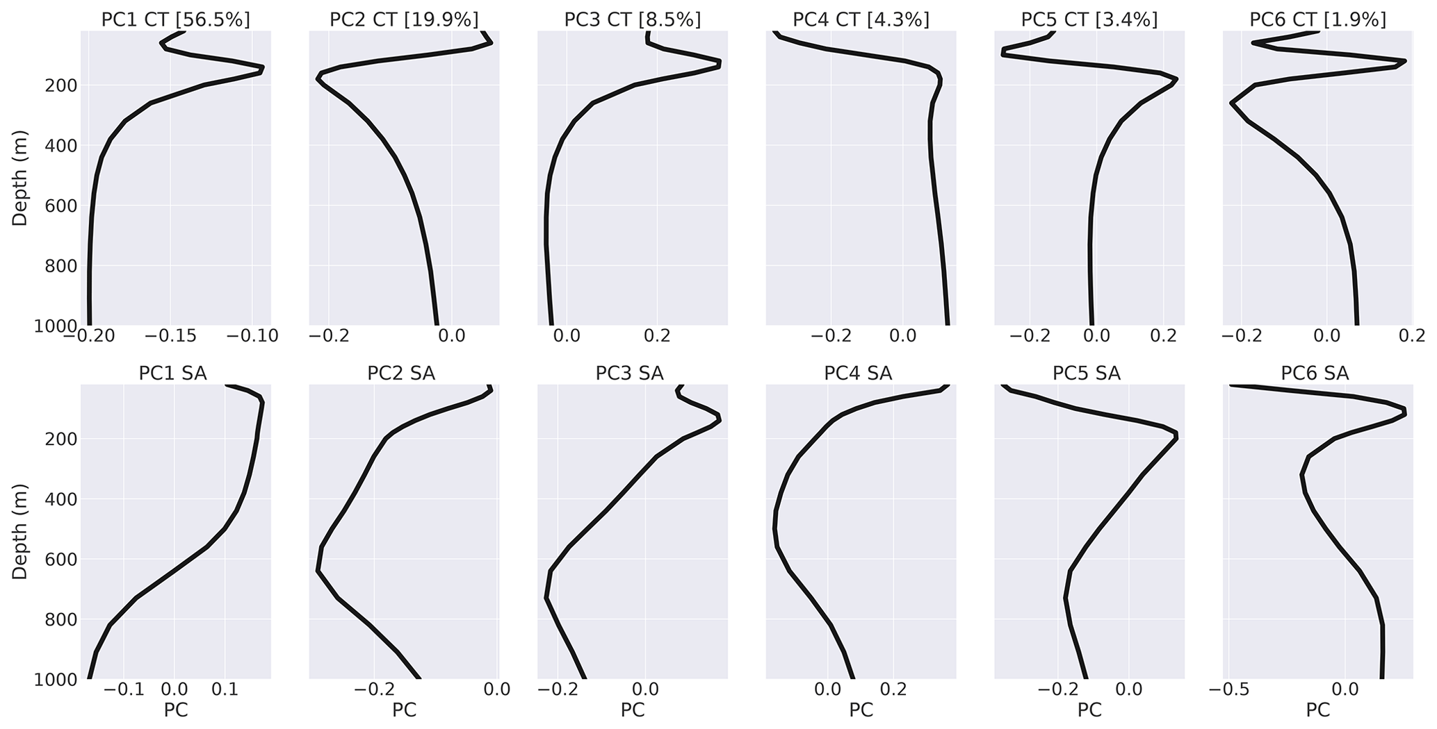
Figure A1The six principal components (PCs) in both temperature and salinity that are used for dimensionality reduction in this study. Each θ–S profile is represented as a linear combination of these six principal components (columns), with a conservative temperature (top row) and absolute salinity (bottom row). The percent variance that is statistically explained by each principal component is shown in each panel title.
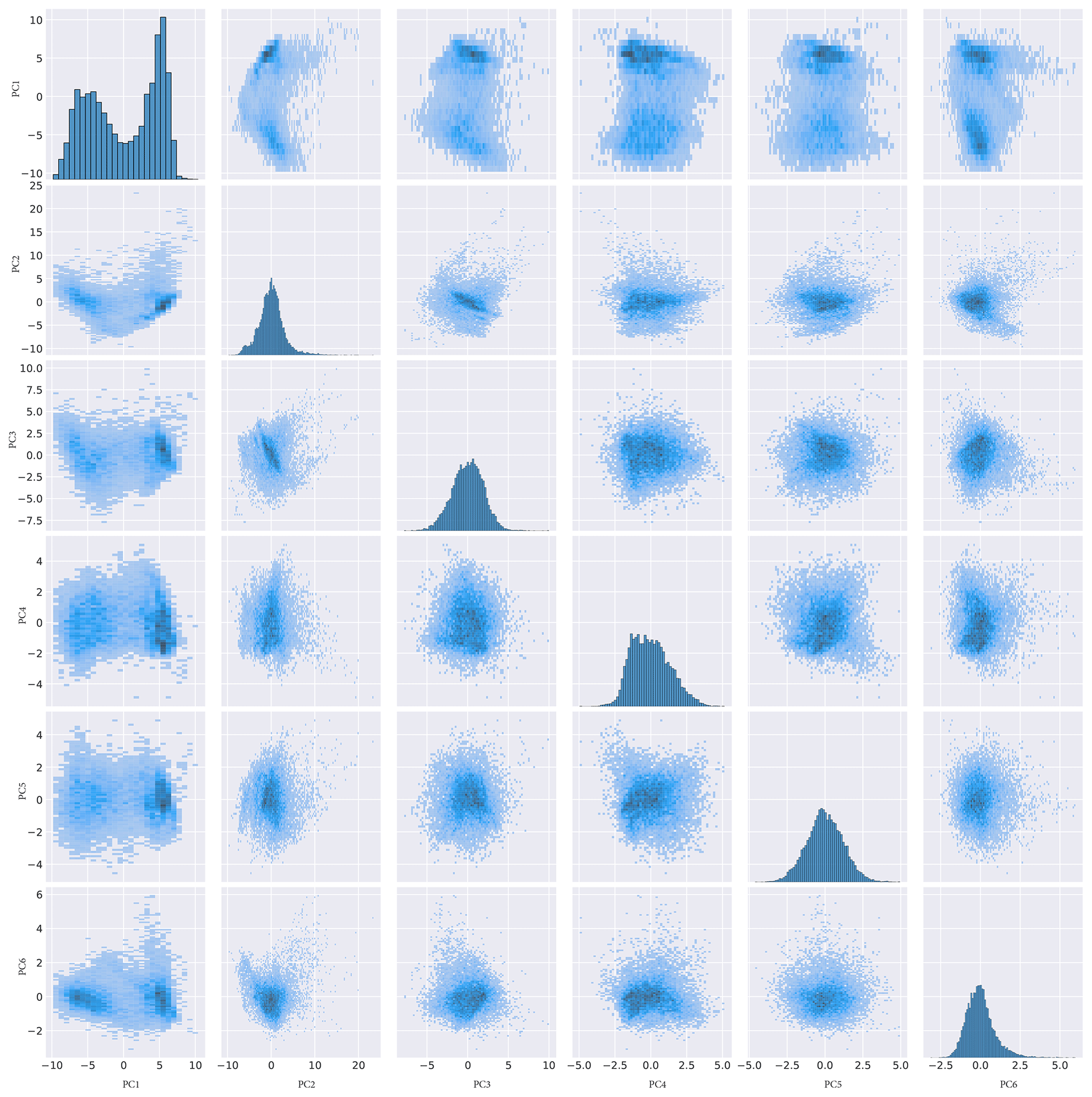
Figure A2The distribution of profiles in PC space. Each row and column represents one of the PCs. The diagonal terms are distributions for each principal component. Diagrams such as this one can be useful for determining which statistical model should be used to describe the data.
A1 Dimension reduction using principal component analysis
Principal component analysis (PCA) attempts to identify a set of eigenfunctions that can efficiently represent a dataset, specifically by representing its variability as a linear combination of these eigenfunctions. In this analysis, we use PCA to represent the vertical variability in the dataset by identifying a set of eigenvectors (i.e. principal components or PCs) that are functions of depth. We find that a six-component representation of the variability in both conservative temperature and absolute salinity retains 95 % of the variability within the dataset, which is acceptable for our application. It is of course possible to increase the number of PCs to retain more of the variability, but this comes at the expense of increased computational complexity. By limiting the number of PCs to six, we strike a balance between computational efficiency and the accuracy of the PC representation of the dataset in terms of its ability to represent the covariance of the data. Because the six-component PC representation only neglects 5 % of the variability, increasing the number of PCs does not appreciably change our results (not shown).
We fit both the PC representation of the profiles and the PCM using a training dataset that is approximately unbiased in terms of spatial coverage. First, we divide the domain into 10∘ by 10∘ bins and select profiles from each bin, where , θ is latitude, and θ0=45∘ S is a reference latitude. The cosine factor helps ensure that the reduced area at higher latitudes is taken into account. The training dataset consists of 13 872 profiles, which is roughly 50 % of the full profile dataset. By using this approximately area-uniform training dataset, we offset the effect of the spatial bias in coverage for both the PC model and the PCM (Fig. 2). That being said, the spatial bias only had a small effect on the PCM; using the full set of profiles, without removing the spatial bias, we arrived at very similar classes and a very similar spatial distribution of classes. The only noticeable differences were around the Prime Meridian, where the presence of repeat hydrographic sections increases the profile density (GO-SHIP reference sections A12 and A13.5). We also tried using larger training datasets with up to 100 % of the profiles; this made no appreciable difference in the final results, suggesting that the 50 % training dataset is sufficiently large to robustly capture the variability. As an alternative approach, we also tried a kernel-based PCA method, but the results were nearly identical.
The six-component PC representation of the system features functions of both conservative temperature and absolute salinity (Fig. A1). Many of the temperature functions feature near-surface temperature inversions; they all feature a rapidly changing near-surface transitioning into a more slowly changing subsurface, as one might expect in ocean profile data in the top 1000 m. Some of the salinity functions also feature such variation, although they are better characterised by more gradual changes between the near-surface and the subsurface. Using this PC representation, we reduce the dimensionality of the data to six PC coefficients. The distribution of those PC coefficients in six-dimensional space shows that a multi-dimensional Gaussian representation is an appropriate way to statistically model this dataset (Fig. A2). It is within this abstract, six-dimensional PC space that we use GMM to find patterns of coherent variability.
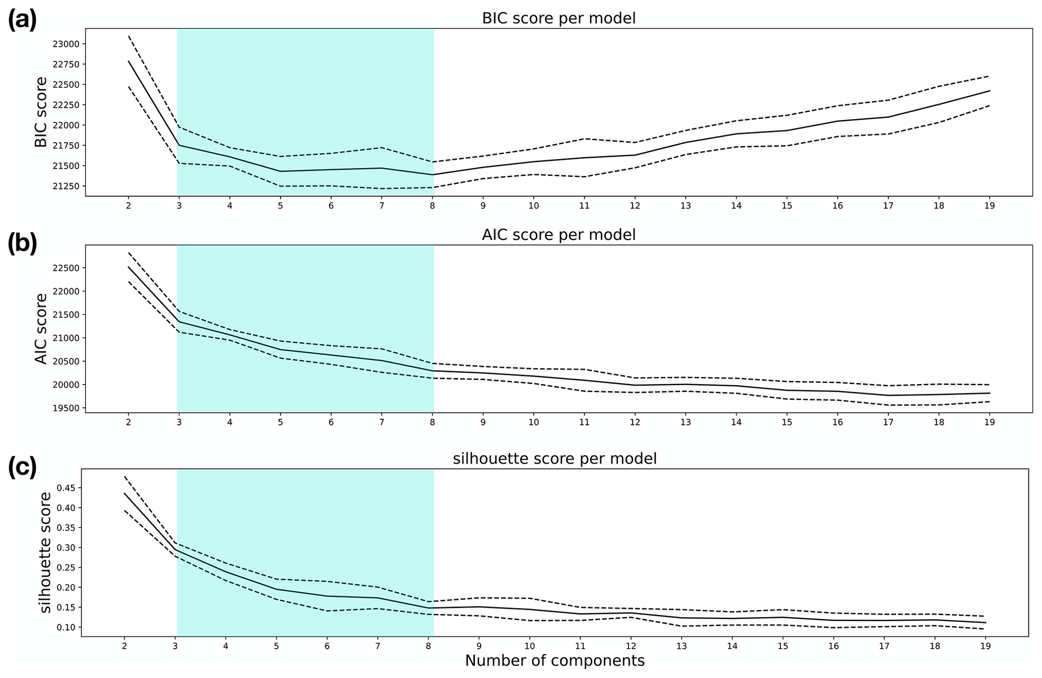
Figure A3Statistical criteria used to guide the selection of the number of components in the GMM algorithm. Shown are the (a) Bayesian information criterion (BIC), (b) the Akaike information criterion (AIC), and (c) the silhouette score. For each K value, these quantities are estimated using 20 random samples from the training dataset. The solid line represents the mean value, and the dashed lines indicate 1 standard deviation on either side. The light green shading indicates the range of classes that we suggest could be supported by these criteria when considered jointly.
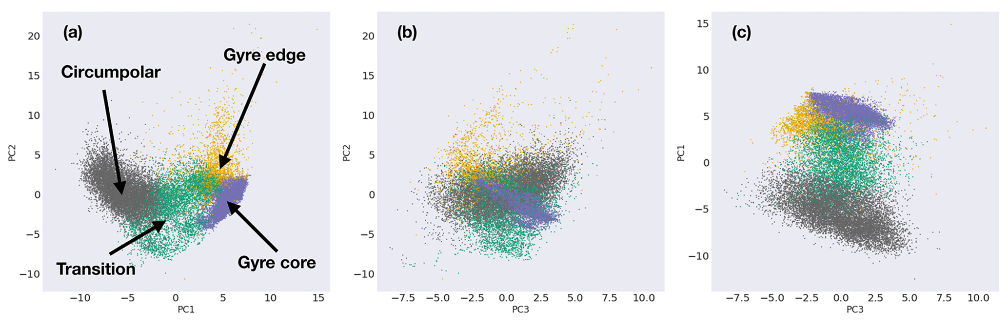
Figure A4Distribution of profiles in 2D slices of the six-dimensional principal component (PC) space through combinations of the first three PCs. Each point in six-dimensional PC space represents a combined temperature and salinity profile. The colour scale indicates the class into which each profile has been sorted by the GMM algorithm, including the circumpolar, transition, gyre edge, and gyre core classes.
A2 Selecting the number of classes
Since oceanographic profile data are highly correlated in space and time, it is unlikely that any classification approach would be able to cleanly and unambiguously identify groups or structures within the dataset that do not have at least some overlap. As such, we approach this classification task with the knowledge that any distinction between ocean profiles will retain some ambiguity. That being said, there are statistical tools that can be used to offer some guidance for making this decision. Two commonly used criteria are the Bayesian information criterion (BIC) (Eq. A1) and Akaike information criterion (AIC) (Eq. A2). Broadly speaking, they both contain a term that measures the agreement of the model with the data, and they both have a penalty term that discourages overfitting. Ideally, one would find a clear minimum in both BIC and AIC at the ideal value of the number of classes, K. In practice, it is rare to find an unambiguous minimum due to the highly correlated nature of the data (e.g. Sonnewald et al., 2019; Jones and Ito, 2019). BIC and AIC can be expressed as
where the log-likelihood is expressed as
Above, ℒ is a measure of likelihood, ηf is the number of independent parameters to be estimated, and N is the number of profiles used in the BIC and AIC training.
In addition to BIC and AIC, we also consider the silhouette coefficient, which is a measure of intra-cluster distance (a) and the mean nearest-cluster distance (b) for each profile (Rousseeuw, 1987). The silhouette coefficient is then . The coefficient has values in the range [−1, 1], where values near −1 indicate that a profile has been assigned “incorrectly” (i.e. it is more similar to a different profile), values near 0 indicate that there is overlap between the clusters, and values near 1 indicate unambiguous classification within the context of the model being used. When working with ocean profile data, which tend to be highly correlated, we do not necessarily expect values close to 1; the silhouette score that is considered “acceptable” varies with dataset and application.
We applied BIC, AIC, and the silhouette score to PCMs of the near-Antarctic data using values of K between 2 and 19. For each value of K, we fit 20 different GMMs using randomly drawn 1000-profile subsets of the training dataset. We used 20 subsets because this empirically gave us stable statistics; i.e. doubling this to 40 made no appreciable difference for the distributions of BIC, AIC, and the silhouette score. When applied to the PC representation of the near-Antarctic data, the combination of BIC, AIC, and silhouette score together indicates that the number of classes lies between K=3 and K=8 (Fig. A3). We find a clear decrease in slope at K=3 across all three metrics, which may be referred to as an “elbow”. As such, the simplest statistical representation of our model consists of three classes, which are physically representative of (1) the Weddell Gyre, (2) the circumpolar regime, and (3) a transition class between the two. By increasing the number of classes to K=4, we see the distinction between the core of the Weddell Gyre and a class along its edge. This increase from K=3 to K=4 is favourable in terms of BIC and AIC, which slightly decrease (indicating greater likelihood), but at the expense of a decrease in silhouette score (indicating more overlap between the classes). Although further increasing K to values greater than 4 improves AIC slightly, it does not improve BIC by much, and it comes at the expense of a decreased silhouette score (worsening overlap). Broadly speaking, the interpretability of our PCM worsens as the silhouette score decreases, as it becomes increasingly difficult to interpret the profile types as being somewhat distinct from one another. For values larger than K=8, BIC begins to increase, indicating that we are in danger of overfitting the data in this regime. As a result of this analysis, we select K=4 as the number of classes in our PCM, striking a balance between the complexity of our representation (i.e. the ability to distinguish the gyre core from the gyre edge) and its interpretability. For completeness, we include Jupyter notebooks for the K=3 and K=8 applications in the archived repository (Jones, 2023).
A3 Profile classification models
Unsupervised classification refers to a broad set of techniques that attempt to sort, group, and/or label a dataset that has not already been sorted, grouped, and/or labelled in some way. As a specific instance of unsupervised classification, Gaussian mixture modelling (GMM) attempts to statistically model the dataset under consideration using a set of multidimensional Gaussian functions (McLachlan and Basford, 1988). When GMM is used to sort ocean profiles, it is sometimes referred to as profile classification model (PCM), for example as seen in Maze et al. (2017). A PCM is “trained” or “fit” by iteratively adjusting the means and covariances of the Gaussian functions, typically using an expectation maximisation approach. We offer a bit more mathematical detail below, adapted from the Appendices of Thomas et al. (2021).
The GMM method attempts to represent the underlying data distribution using a set of K Gaussian functions in D dimensions (in our case D=3):
where is a vector in the PC space, is the centre of the Gaussian distribution expressed in vector form, is the covariance matrix, and is its determinant. The covariance matrix determines the orientation of the Gaussian ellipsoids in PC space. We statistically represent the dataset using the following probability distribution:
where λk is the weight associated with the kth Gaussian. The GMM process iteratively adjusts λk, μk, and Σk to decrease the model–data misfit, which is called expectation maximisation and is described in more detail in the next paragraph.
The first K clusters are created randomly. Next, the set of Gaussians is iteratively adjusted (Eqs. A6, A7, and A8) until it reaches a local minimum in the cost function. The expectation of the model given the data is increased by updating the weights λk, means μk, and covariance matrices Σk in the following way:
where cn is the classification of the nth cluster, which could be any one of the K clusters. The GMM algorithm repeats this process until the parameters have converged.
As discussed in Sect. A1, we use a spatially unbiased training dataset to estimate the hyper-parameters of our GMM, ensuring that the resulting PCM is generally applicable across the entire spatial domain, rather than being specifically tuned to areas where there happen to be a large number of profiles (e.g. along ship-track repeat sections).
Each profile is assigned a posterior probability distribution across the K clusters (Eq. A9). This uncertainty information is one of the useful features of GMM. The probability takes the form
To label a dataset, each profile is assigned a label from the cluster that it would be most likely to be generated by in a statistical sense (Eq. A10):
A4 PCM applied in PC space
The four-class PCM identifies (1) a circumpolar class, (2) a transition class between the circumpolar waters and the Weddell Gyre, (3) waters on the edge of the gyre, and (4) waters in the core of the gyre. These clusters are identified in a six-dimensional PC space, in which the dimensions are the principal component coefficients and each profile is represented by a single point. In a 3D projection of the six-dimensional PC space, which statistically explains about 85 % of the variability, we see a covariance structure that may be described as “two wings and a bridge between them”. The four-class model highlights these two “wings”, namely a circumpolar wing and a gyre wing, separated by a transition “bridge” between the two wings (Fig. A4). If we imagine a stack of water masses transforming from more circumpolar-type to more gyre-type waters, this transformation would be represented by crossing the “bridge” from the circumpolar wing to the gyre wing. Much of the variability is contained in the first principal component (roughly 60 %), which represents aspects of large-scale salt stratification.
The initial set of profiles used in this study covers the South Atlantic and part of the Indian Ocean (Sect. 2.1). As a first classification step, we applied the PCM technique to this dataset in order to identify a coherent set of near-Antarctic profiles. We chose to use this data-driven approach for consistency with the rest of our analysis, although in practice selecting all profiles south of the PF would not substantially change our results, especially not those closer to the Weddell Gyre. Starting with the cleaned and prepared South Atlantic and Indian Ocean data, we followed the PCM procedure described in Sect. 2. First, we reduced the dimensionality of the data using a six-component PCA, retaining 95 % of the variability. We used the elbow method with both BIC (Eq. A1) and AIC (Eq. A2) to estimate the optimal number of classes K, which in this case was K=5; at K=5, the slope of both the mean BIC and AIC curves changes considerably, and BIC does not change much for K>5.
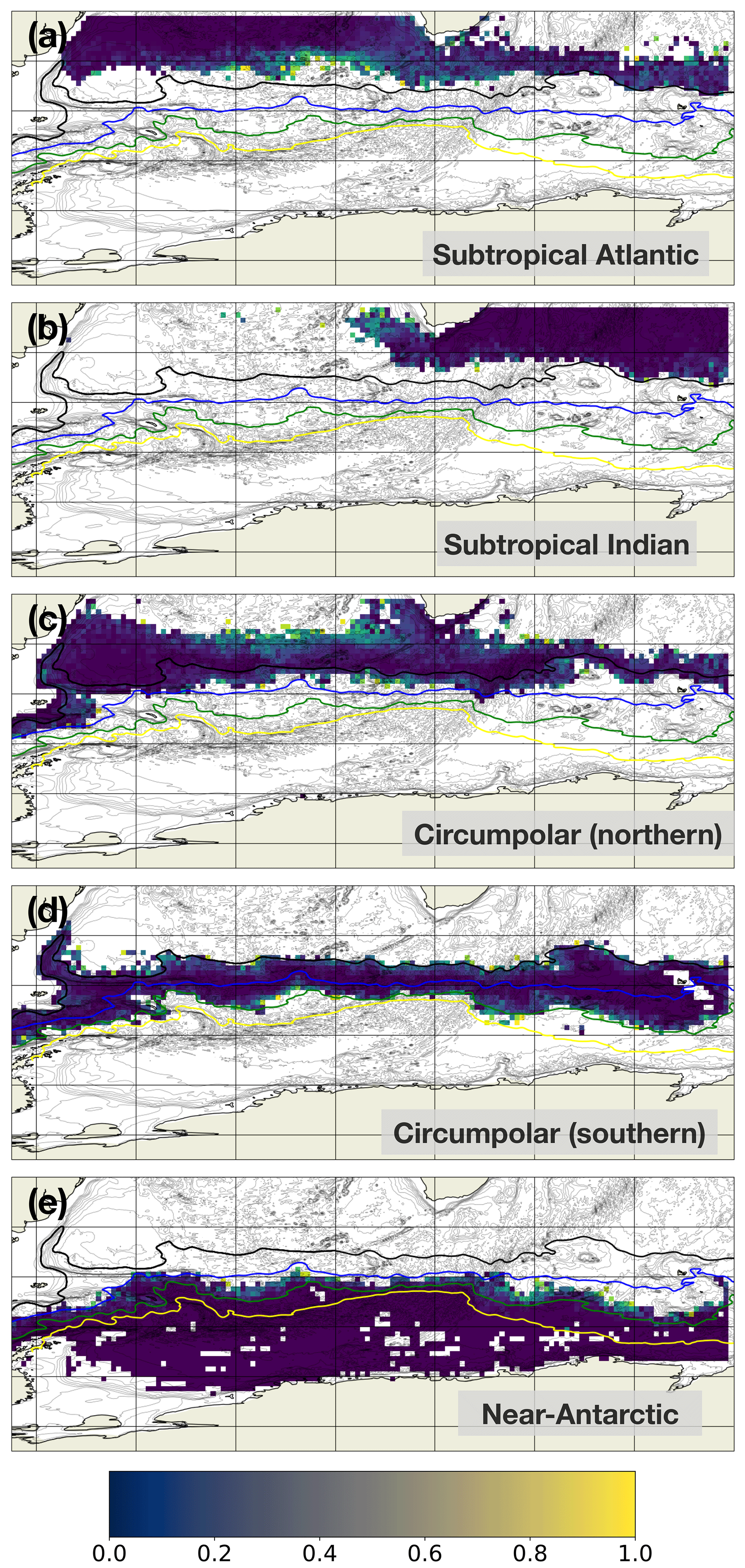
Figure B1A five-class PCM of the initial dataset. The quantity shown is the I-metric, which is the probability that a profile is near a boundary between classes, as described in Sect. 3.2. Also shown are fronts of the ACC, as described in Fig. 5. The rest of this study is essentially a “sub-classification” of the near-Antarctic class.
The five-component PCM consists of these profile types: (1) subtropical Atlantic, (2) subtropical Indian, (3) circumpolar (more northern), (4) circumpolar (more southern), and (5) near-Antarctic (Fig. B1). There are some excursions of the circumpolar (southern) class south of the PF, especially in the easternmost part of the domain, but the near-Antarctic class mostly consists of those profiles that are located south of the PF. The main analysis in this paper is a sub-classification of the “near-Antarctic” profiles.
The dataset used in this study consists of profiles taken by Argo floats (https://doi.org/10.17882/42182, Argo, 2020) and ship-based CTDs as recorded in the World Ocean Database (https://www.ncei.noaa.gov/sites/default/files/2020-04/wod_intro_0.pdf, last access: 14 June 2023, Boyer, 2018). SOSE iteration-100 data are available from the Scripps Institution of Oceanography (http://sose.ucsd.edu/sose_stateestimation_data_05to10.html, last access: 4 June 2023, Mazloff, 2023). CDRv4 is available via NSIDC (https://doi.org/10.7265/efmz-2t65, Meier et al., 2021), and Polar Pathfinder sea ice drift data are also available via NSIDC (https://doi.org/10.5067/INAWUWO7QH7B, Tschudi et al., 2019). The code used to perform this analysis and produce the figures used in the paper is available via Zenodo (https://doi.org/10.5281/zenodo.7465388, Jones, 2023). The full dataset used in this work is also available via Zenodo (https://doi.org/10.5281/zenodo.7468656, Jones and Zhou, 2022). A labelled dataset is also available via Zenodo (https://doi.org/10.5281/zenodo.7465132, Jones and Zhou, 2022b).
DCJ designed the study, wrote the software to carry out the analysis, and created the figures. DCJ, MS, and IR collaborated on methods. SZ provided the cleaned, processed profile dataset and the stress-driven upwelling estimate. UH, IR, MPM, AJSM, and ACNG contributed to the interpretation of the classes and helped put the results into the wider context of the literature. All authors contributed to the writing of the paper.
The contact author has declared that none of the authors has any competing interests.
Publisher's note: Copernicus Publications remains neutral with regard to jurisdictional claims in published maps and institutional affiliations.
This article is part of the special issue “The Weddell Sea and the ocean off Dronning Maud Land: unique oceanographic conditions shape circumpolar and global processes – a multi-disciplinary study (OS/BG/TC inter-journal SI)”. It is not associated with a conference.
We thank Erin Thomas, Earle Wilson, Drew Gronewold, and two anonymous reviewers for discussions that helped improve the quality of this work. Thanks to Jason Lewis (Mind Amend) for providing music for focus and productivity. We used the scikit-learn Python module for unsupervised classification (Pedregosa et al., 2011).
This research has been supported by UK Research and Innovation (grant no. MR/T020822/1) and the European Commission, Horizon 2020 Framework Programme (grant no. 821001).
This paper was edited by Markus Janout and reviewed by two anonymous referees.
Abrahamsen, E. P., Meijers, A. J. S., Polzin, K. L., Naveira Garabato, A. C., King, B. A., Firing, Y. L., Sallée, J.-B., Sheen, K. L., Gordon, A. L., Huber, B. A., and Meredith, M. P.: Stabilization of dense Antarctic water supply to the Atlantic Ocean overturning circulation, Nat. Clim. Change, 9, 742–746, https://doi.org/10.1038/s41558-019-0561-2, 2019. a
Argo: Argo float data and metadata from Global Data Assembly Centre (Argo GDAC), SEANOE [data set], https://doi.org/10.17882/42182, 2020. a
Belkina, A. C., Ciccolella, C. O., Anno, R., Halpert, R., Spidlen, J., and Snyder-Cappione, J. E.: Automated optimized parameters for T-distributed stochastic neighbor embedding improve visualization and analysis of large datasets, Nat. Commun., 10, 5415, https://doi.org/10.1038/s41467-019-13055-y, 2019. a
Boehme, L. and Rosso, I.: Classifying Oceanographic Structures in the Amundsen Sea, Antarctica, Geophys. Res. Lett., 48, e2020GL089412, https://doi.org/10.1029/2020GL089412, 2021. a
Boyer, T. P., Baranova, O. K., Coleman, C., Garcia, H. E., Grodsky, A., Locarnini, R. A., Mishonov, A. V., Paver, C. R., Reagan, J. R., Seidov, D., Smolyar, I. V., Weathers, K., Zweng, M. M.: World Ocean Database 2018, A.V. Mishonov, Technical Ed., NOAA Atlas NESDIS 87, [data set], https://www.ncei.noaa.gov/sites/default/files/2020-04/wod_intro_0.pdf (last access: 14 June 2023), 2018. a
Campbell, E. C., Wilson, E. A., Moore, G. W. K., Riser, S. C., Brayton, C. E., Mazloff, M. R., and Talley, L. D.: Antarctic offshore polynyas linked to Southern Hemisphere climate anomalies, Nature, 570, 319–325, https://doi.org/10.1038/s41586-019-1294-0, 2019. a
Chapman, C. C., Lea, M.-A., Meyer, A., Sallée, J.-B., and Hindell, M.: Defining Southern Ocean fronts and their influence on biological and physical processes in a changing climate, Nat. Clim. Change, 10, 209–219, https://doi.org/10.1038/s41558-020-0705-4, 2020. a, b
Couchman, M. M. P., Wynne-Cattanach, B., Alford, M. H., Caulfield, C.-C. P., Kerswell, R. R., MacKinnon, J. A., and Voet, G.: Data-Driven Identification of Turbulent Oceanic Mixing From Observational Microstructure Data, Geophys. Res. Lett., 48, e2021GL094978, https://doi.org/10.1029/2021GL094978, 2021. a
Desbruyères, D., Chafik, L., and Maze, G.: A shift in the ocean circulation has warmed the subpolar North Atlantic Ocean since 2016, Communications Earth & Environment, 2, 1–9, https://doi.org/10.1038/s43247-021-00120-y, 2021. a
Dotto, T. S., Naveira Garabato, A., Bacon, S., Tsamados, M., Holland, P. R., Hooley, J., Frajka-Williams, E., Ridout, A., and Meredith, M. P.: Variability of the Ross Gyre, Southern Ocean: Drivers and Responses Revealed by Satellite Altimetry, Geophys. Res. Lett., 45, 6195–6204, https://doi.org/10.1029/2018GL078607, 2018. a, b, c
Fahrbach, E., Rohardt, G., Schröder, M., and Strass, V.: Transport and structure of the Weddell Gyre, Ann. Geophys., 12, 840–855, https://doi.org/10.1007/s00585-994-0840-7, 1994. a, b
Forget, G., Campin, J.-M., Heimbach, P., Hill, C. N., Ponte, R. M., and Wunsch, C.: ECCO version 4: an integrated framework for non-linear inverse modeling and global ocean state estimation, Geosci. Model Dev., 8, 3071–3104, https://doi.org/10.5194/gmd-8-3071-2015, 2015. a
Foster, T. D. and Carmack, E. C.: Frontal zone mixing and Antarctic Bottom water formation in the southern Weddell Sea, Deep-Sea Research and Oceanographic Abstracts, 23, 301–317, https://doi.org/10.1016/0011-7471(76)90872-X, 1976. a
Gill, A.: Circulation and bottom water production in the Weddell Sea, Deep-Sea Research and Oceanographic Abstracts, 20, 111–140, https://doi.org/10.1016/0011-7471(73)90048-X, 1973. a
Gordon, A. L. and Huber, B. A.: Southern ocean winter mixed layer, J. Geophys. Res., 95, 11655–11672, https://doi.org/10.1029/JC095iC07p11655, 1990. a
Gordon, A. L.: Deep Antarctic Convection West of Maud Rise, J. Phys. Oceanogr., 8, 600–612, https://doi.org/10.1175/1520-0485(1978)008<0600:DACWOM>2.0.CO;2, 1978. a
Gordon, A. L., Visbeck, M., and Huber, B.: Export of Weddell Sea deep and bottom water, J. Geophys. Res.-Oceans, 106, 9005–9017, https://doi.org/10.1029/2000JC000281, 2001. a
Haumann, F. A., Gruber, N., Münnich, M., Frenger, I., and Kern, S.: Sea-ice transport driving Southern Ocean salinity and its recent trends, Nature, 537, 89–92, https://doi.org/10.1038/nature19101, 2016. a, b
Held, I.: The gap between simulation and understanding in climate modeling, B. Am. Meteorol. Soc., 86, 1609–1614, 2005. a, b
Houghton, I. A. and Wilson, J. D.: El Niño Detection Via Unsupervised Clustering of Argo Temperature Profiles, J. Geophys. Res.-Oceans, 125, e2019JC015947, https://doi.org/10.1029/2019JC015947, 2020. a
IPCC: The Ocean and Cryosphere in a Changing Climate: Special Report of the Intergovernmental Panel on Climate Change, Cambridge University Press, https://doi.org/10.1017/9781009157964, 2022. a
Johnson, G. C.: Quantifying Antarctic Bottom Water and North Atlantic Deep Water volumes, J. Geophys. Res.-Oceans, 113, C05027, https://doi.org/10.1029/2007JC004477, 2008. a
Johnson, G. C., Purkey, S. G., and Toole, J. M.: Reduced Antarctic meridional overturning circulation reaches the North Atlantic Ocean, Geophys. Res. Lett., 35, L22601, https://doi.org/10.1029/2008GL035619, 2008. a
Jones, D.: so-wise/weddell_gyre_clusters: Third release, https://doi.org/10.5281/zenodo.7465388, 2023. a, b
Jones, D. and Zhou, S.: SO-WISE South Atlantic Ocean and Indian Ocean Observational Constraints, Zenodo, https://doi.org/10.5281/zenodo.7468656, 2022. a, b
Jones, D. C. and Ito, T.: Gaussian mixture modeling describes the geography of the surface carbon budget, in: Proceedings of the 9th International Workshop on Climate Informatics, p. 6, Paris, France, https://doi.org/10.5065/y82j-f154, 2019. a, b
Jones, D. C., Holt, H. J., Meijers, A. J. S., and Shuckburgh, E.: Unsupervised Clustering of Southern Ocean Argo Float Temperature Profiles, J. Geophys. Res.-Oceans, 40, 390–402, https://doi.org/10.1029/2018JC014629, 2019. a, b
Jones, D. and Zhou, S.: South Atlantic Ocean profile dataset: identification of near-Antarctic profiles using unsupervised classification, Zenodo [data set], https://doi.org/10.5281/zenodo.7465132, 2022b. a
Jullion, L., Garabato, A. C. N., Bacon, S., Meredith, M. P., Brown, P. J., Torres-Valdés, S., Speer, K. G., Holland, P. R., Dong, J., Bakker, D., Hoppema, M., Loose, B., Venables, H. J., Jenkins, W. J., Messias, M.-J., and Fahrbach, E.: The contribution of the Weddell Gyre to the lower limb of the Global Overturning Circulation, J. Geophys. Res.-Oceans, 119, 3357–3377, https://doi.org/10.1002/2013JC009725, 2014. a, b
Kaiser, B. E., Saenz, J. A., Sonnewald, M., and Livescu, D.: Automated identification of dominant physical processes, Eng. Appl. Artif. Intell., 116, 105496, https://doi.org/10.1016/j.engappai.2022.105496, 2022. a
Killworth, P.: An equivalent-barotropic mode in the Fine Resolution Antarctic Model, J. Phys. Oceanogr., 22, 1379–1387, 1992. a
Killworth, P. D.: Deep convection in the World Ocean, Rev. Geophys., 21, 1–26, https://doi.org/10.1029/RG021i001p00001, 1983. a
Kim, Y. S. and Orsi, A. H.: On the Variability of Antarctic Circumpolar Current Fronts Inferred from 1992–2011 Altimetry*, J. Phys. Oceanogr., 44, 3054–3071, https://doi.org/10.1175/JPO-D-13-0217.1, 2014. a, b
Kobak, D. and Berens, P.: The art of using t-SNE for single-cell transcriptomics, Nat. Commun., 10, 5416, https://doi.org/10.1038/s41467-019-13056-x, 2019. a
Krupitsky, A., Kamenkovich, V., Naik, N., and Cane, M.: A linear equivalent barotropic model of the Antarctic Circumpolar Current with realistic coastlines and bottom topography, J. Phys. Oceanogr., 26, 1803–1824, 1996. a
Maaten, L. v. d. and Hinton, G.: Visualizing Data using t-SNE, J. Mach. Learn. Res., 9, 2579–2605, 2008. a
Marshall, D.: Influence of topography on the large-scale ocean circulation, J. Phys. Oceanogr., 25, 1622–1635, 1995. a
Martinson, D. G.: Evolution of the southern ocean winter mixed layer and sea ice: Open ocean deepwater formation and ventilation, J. Geophys. Res.-Oceans, 95, 11641–11654, https://doi.org/10.1029/JC095iC07p11641, 1990. a
Maze, G., Mercier, H., Fablet, R., Tandeo, P., Radcenco, M. L., Lenca, P., Feucher, C., and Le Goff, C.: Coherent heat patterns revealed by unsupervised classification of Argo temperature profiles in the North Atlantic Ocean, Prog. Oceanogr., 151, 275–292, https://doi.org/10.1016/j.pocean.2016.12.008, 2017. a, b
Mazloff, M. R., Heimbach, P., and Wunsch, C.: An Eddy-Permitting Southern Ocean State Estimate, J. Phys. Oceanogr., 40, 880–899, https://doi.org/10.1175/2009jpo4236.1, 2010. a, b
Mazloff, M.: Scripps Institution of Oceanography, Southern Ocean State Estimate [Iteration 100], [data set], http://sose.ucsd.edu/sose_stateestimation_data_05to10.html last access: 4 June 2023. a
McDougall, T. and Barker, P.: Getting started with TEOS-10 and the Gibbs Seawater (GSW) Oceanographic Toolbox, SCOR/IAPSO WG127, ISBN 978-0-646-55621-5, 2011. a
McLachlan, G. and Basford, K.: Mixture Models: Inference and Applications to Clustering, Dekker, ISBN-13 9780824776916, 1988. a
Meier, W. N., Fetterer, F., Windnagel, A. K., and Stewart, J. S.: NOAA/NSIDC Climate Data Record of Passive Microwave Sea Ice Concentration, Version 4 [data set], Boulder, Colorado USA, National Snow and Ice Data Center, https://doi.org/10.7265/efmz-2t65, 2021. a
Meijers, A. J. S., Klocker, A., Bindoff, N. L., Williams, G. D., and Marsland, S. J.: The circulation and water masses of the Antarctic shelf and continental slope between 30 and 80∘ E, Deep-Sea Res. Pt. II, 57, 723–737, https://doi.org/10.1016/j.dsr2.2009.04.019, 2010. a
Naveira Garabato, A. C., McDonagh, E. L., Stevens, D. P., Heywood, K. J., and Sanders, R. J.: On the export of Antarctic Bottom Water from the Weddell Sea, Deep-Sea Res. Pt. II, 49, 4715–4742, https://doi.org/10.1016/S0967-0645(02)00156-X, 2002. a
Naveira Garabato, A. C., Zika, J. D., Jullion, L., Brown, P. J., Holland, P. R., Meredith, M. P., and Bacon, S.: The thermodynamic balance of the Weddell Gyre, Geophys. Res. Lett., 43, 317–325, https://doi.org/10.1002/2015GL066658, 2016. a, b
Park, Y.-H., Charriaud, E., Craneguy, P., and Kartavtseff, A.: Fronts, transport, and Weddell Gyre at 30∘ E between Africa and Antarctica, J. Geophys. Res.-Oceans, 106, 2857–2879, https://doi.org/10.1029/2000JC900087, 2001. a
Patmore, R. D., Holland, P. R., Munday, D. R., Garabato, A. C. N., Stevens, D. P., and Meredith, M. P.: Topographic Control of Southern Ocean Gyres and the Antarctic Circumpolar Current: A Barotropic Perspective, J. Phys. Oceanogr., 49, 3221–3244, https://doi.org/10.1175/JPO-D-19-0083.1, 2019. a, b
Patterson, S. L. and Sievers, H. A.: The Weddell-Scotia Confluence, J. Phys. Oceanogr., 10, 1584–1610, https://doi.org/10.1175/1520-0485(1980)010<1584:TWSC>2.0.CO;2, 1980. a, b, c
Pauthenet, E., Roquet, F., Madec, G., and Nerini, D.: A linear decomposition of the Southern Ocean thermohaline structure, J. Phys. Oceanogr., 47, 29–47, https://doi.org/10.1175/JPO-D-16-0083.s1, 2017. a
Pedregosa, F., Varoquaux, G., Gramfort, A., Michel, V., Thirion, B., Grisel, O., Blondel, M., Prettenhofer, P., Weiss, R., Dubourg, V., Vanderplas, J., Passos, A., Cournapeau, D., Brucher, M., Perrot, M., and Duchesnay, E.: Scikit-learn: Machine Learning in Python, J. Mach. Learn. Res., 12, 2825–2830, 2011. a
Reeve, K. A., Boebel, O., Kanzow, T., Strass, V., Rohardt, G., and Fahrbach, E.: A gridded data set of upper-ocean hydrographic properties in the Weddell Gyre obtained by objective mapping of Argo float measurements, Earth Syst. Sci. Data, 8, 15–40, https://doi.org/10.5194/essd-8-15-2016, 2016. a, b
Reeve, K. A., Boebel, O., Strass, V., Kanzow, T., and Gerdes, R.: Horizontal circulation and volume transports in the Weddell Gyre derived from Argo float data, Prog. Oceanogr., 175, 263–283, https://doi.org/10.1016/j.pocean.2019.04.006, 2019. a, b
Rintoul, S. R. and Garabato, A. C. N.: Chapter 18 – Dynamics of the Southern Ocean Circulation, in: Ocean Circulation and Climate, edited by: Siedler, G., Griffies, S. M., Gould, J., and Church, J. A., Vol. 103 of International Geophysics, 471–492, Academic Press, https://doi.org/10.1016/B978-0-12-391851-2.00018-0, 2013. a
Roquet, F., Ferreira, D., Caneill, R., Schlesinger, D., and Madec, G.: Unique thermal expansion properties of water key to the formation of sea ice on Earth, Sci. Adv., 8, eabq0793, https://doi.org/10.1126/sciadv.abq0793, 2022. a
Rosso, I., Mazloff, M. R., Talley, L. D., Purkey, S. G., Freeman, N. M., and Maze, G.: Water Mass and Biogeochemical Variability in the Kerguelen Sector of the Southern Ocean: A Machine Learning Approach for a Mixing Hot Spot, J. Geophys. Res.-Oceans, 125, e2019JC015877, https://doi.org/10.1029/2019JC015877, 2020. a
Rousseeuw, P. J.: Silhouettes: A graphical aid to the interpretation and validation of cluster analysis, J. Comput. Appl. Math., 20, 53–65, https://doi.org/10.1016/0377-0427(87)90125-7, 1987. a
Sambe, F. and Suga, T.: Unsupervised Clustering of Argo Temperature and Salinity Profiles in the Mid-Latitude Northwest Pacific Ocean and Revealed Influence of the Kuroshio Extension Variability on the Vertical Structure Distribution, J. Geophys. Res.-Oceans, 127, e2021JC018138, https://doi.org/10.1029/2021JC018138, 2022. a
Schmidtko, S., Heywood, K. J., Thompson, A. F., and Aoki, S.: Multidecadal warming of Antarctic waters, Science, 346, 1227–1231, https://doi.org/10.1126/science.1256117, 2014. a
Sokolov, S. and Rintoul, S. R.: Circumpolar structure and distribution of the Antarctic Circumpolar Current fronts: 2. Variability and relationship to sea surface height, J. Geophys. Res.-Oceans, 114, C11019, https://doi.org/10.1029/2008JC005248, 2009. a
Sonnewald, M. and Lguensat, R.: Revealing the Impact of Global Heating on North Atlantic Circulation Using Transparent Machine Learning, J. Adv. Model. Earth Sy., 13, e2021MS002496, https://doi.org/10.1029/2021MS002496, 2021. a
Sonnewald, M., Wunsch, C., and Heimbach, P.: Unsupervised Learning Reveals Geography of Global Ocean Dynamical Regions, Earth Space Sci., 6, 784–794, https://doi.org/10.1029/2018EA000519, 2019. a, b
Sonnewald, M., Dutkiewicz, S., Hill, C., and Forget, G.: Elucidating ecological complexity: Unsupervised learning determines global marine eco-provinces, Sci. Adv., 6, eaay4740, https://doi.org/10.1126/sciadv.aay4740, 2020. a
Sonnewald, M., Lguensat, R., Jones, D. C., Dueben, P. D., Brajard, J., and Balaji, V.: Bridging observations, theory and numerical simulation of the ocean using machine learning, Environ. Res. Lett., 16, 073008, https://doi.org/10.1088/1748-9326/ac0eb0, 2021. a, b
Thomas, E. E. and Müller, M.: Characterizing vertical upper ocean temperature structures in the European Arctic through unsupervised machine learning, Ocean Model., 177, 102092, https://doi.org/10.1016/j.ocemod.2022.102092, 2022. a
Thomas, S. D. A., Jones, D. C., Faul, A., Mackie, E., and Pauthenet, E.: Defining Southern Ocean fronts using unsupervised classification, Ocean Sci., 17, 1545–1562, https://doi.org/10.5194/os-17-1545-2021, 2021. a, b, c, d, e
Thompson, A. F., Stewart, A. L., Spence, P., and Heywood, K. J.: The Antarctic Slope Current in a Changing Climate, Rev. Geophys., 56, 741–770, https://doi.org/10.1029/2018RG000624, 2018. a
Thomson, R. E. and Fine, I. V.: Estimating Mixed Layer Depth from Oceanic Profile Data, J. Atmos. Ocean. Tech., 20, 319–329, https://doi.org/10.1175/1520-0426(2003)020<0319:EMLDFO>2.0.CO;2, 2003. a, b
Tschudi, M., Meier, W., Stewart, N. J. S., Fowler, C., and Maslanik, J.: Polar Pathfinder Daily 25 km EASE-Grid Sea Ice Motion Vectors, Version 4 [data set], Boulder, Colorado USA. NASA National Snow and Ice Data Center Distributed Active Archive Center, https://doi.org/10.5067/INAWUWO7QH7B, 2019. a
van der Maaten, L. and Hinton, G.: Visualizing Data using t-SNE, J. Mach. Learn. Res., 9, 2579–2605, 2008. a
Vernet, M., Geibert, W., Hoppema, M., Brown, P. J., Haas, C., Hellmer, H. H., Jokat, W., Jullion, L., Mazloff, M., Bakker, D. C. E., Brearley, J. A., Croot, P., Hattermann, T., Hauck, J., Hillenbrand, C.-D., Hoppe, C. J. M., Huhn, O., Koch, B. P., Lechtenfeld, O. J., Meredith, M. P., Naveira Garabato, A. C., Nöthig, E.-M., Peeken, I., Rutgers van der Loeff, M. M., Schmidtko, S., Schröder, M., Strass, V. H., Torres-Valdés, S., and Verdy, A.: The Weddell Gyre, Southern Ocean: Present Knowledge and Future Challenges, Rev. Geophys., 57, 623–708, https://doi.org/10.1029/2018RG000604, 2019. a, b, c, d, e, f, g, h, i
Whitworth, T., Nowlin, W. D., Orsi, A. H., Locarnini, R. A., and Smith, S. G.: Weddell Sea shelf water in the Bransfield Strait and Weddell-Scotia Confluence, Deep-Sea Res. Pt. I, 41, 629–641, https://doi.org/10.1016/0967-0637(94)90046-9, 1994. a, b
Wilson, E. A., Thompson, A. F., Stewart, A. L., and Sun, S.: Bathymetric Control of Subpolar Gyres and the Overturning Circulation in the Southern Ocean, J. Phys. Oceanogr., 52, 205–223, https://doi.org/10.1175/JPO-D-21-0136.1, 2022. a
Xia, X., Hong, Y., Du, Y., and Xiu, P.: Three Types of Antarctic Intermediate Water Revealed by a Machine Learning Approach, Geophys. Res. Lett., 49, e2022GL099445, https://doi.org/10.1029/2022GL099445, 2022. a
Zhang, Q., Qian, C., and Dong, C.: A machine learning approach to quality-control Argo temperature data, Atmos. Ocean. Sci. Lett., https://doi.org/10.1016/j.aosl.2022.100292, online first, 2022. a
- Abstract
- Introduction
- Data and methods
- Results
- Discussion
- Conclusions
- Appendix A: Details of principal component analysis (PCA) and profile classification modelling (PCM)
- Appendix B: Five-class PCM of entire South Atlantic Ocean and Indian Ocean dataset
- Code and data availability
- Author contributions
- Competing interests
- Disclaimer
- Special issue statement
- Acknowledgements
- Financial support
- Review statement
- References