the Creative Commons Attribution 4.0 License.
the Creative Commons Attribution 4.0 License.
 | 26 May 2023
Ocean color algorithm for the retrieval of the particle size distribution and carbon-based phytoplankton size classes using a two-component coated-sphere backscattering model
Tihomir S. Kostadinov
Lisl Robertson Lain
Christina Eunjin Kong
Xiaodong Zhang
Stéphane Maritorena
Stewart Bernard
Hubert Loisel
Daniel S. F. Jorge
Ekaterina Kochetkova
Shovonlal Roy
Bror Jonsson
Victor Martinez-Vicente
Shubha Sathyendranath
The particle size distribution (PSD) of suspended particles in near-surface seawater is a key property linking biogeochemical and ecosystem characteristics with optical properties that affect ocean color remote sensing. Phytoplankton size affects their physiological characteristics and ecosystem and biogeochemical roles, e.g., in the biological carbon pump, which has an important role in the global carbon cycle and thus climate. It is thus important to develop capabilities for measurement and predictive understanding of the structure and function of oceanic ecosystems, including the PSD, phytoplankton size classes (PSCs), and phytoplankton functional types (PFTs). Here, we present an ocean color satellite algorithm for the retrieval of the parameters of an assumed power-law PSD. The forward optical model considers two distinct particle populations: phytoplankton and non-algal particles (NAPs). Phytoplankton are modeled as coated spheres following the Equivalent Algal Populations (EAP) framework, and NAPs are modeled as homogeneous spheres. The forward model uses Mie and Aden–Kerker scattering computations, for homogeneous and coated spheres, respectively, to model the total particulate spectral backscattering coefficient as the sum of phytoplankton and NAP backscattering. The PSD retrieval is achieved via spectral angle mapping (SAM), which uses backscattering end-members created by the forward model. The PSD is used to retrieve size-partitioned absolute and fractional phytoplankton carbon concentrations (i.e., carbon-based PSCs), as well as particulate organic carbon (POC), using allometric coefficients. This model formulation also allows the estimation of chlorophyll a concentration via the retrieved PSD, as well as percent of backscattering due to NAPs vs. phytoplankton. The PSD algorithm is operationally applied to the merged Ocean Colour Climate Change Initiative (OC-CCI) v5.0 ocean color data set. Results of an initial validation effort are also presented using PSD, POC, and picophytoplankton carbon in situ measurements. Validation results indicate the need for an empirical tuning for the absolute phytoplankton carbon concentrations; however these results and comparison with other phytoplankton carbon algorithms are ambiguous as to the need for the tuning. The latter finding illustrates the continued need for high-quality, consistent, large global data sets of PSD, phytoplankton carbon, and related variables to facilitate future algorithm improvements.
Please read the corrigendum first before continuing.
-
Notice on corrigendum
The requested paper has a corresponding corrigendum published. Please read the corrigendum first before downloading the article.
-
Article
(16791 KB)
- Corrigendum
-
Supplement
(16001 KB)
-
The requested paper has a corresponding corrigendum published. Please read the corrigendum first before downloading the article.
- Article
(16791 KB) - Full-text XML
- Corrigendum
-
Supplement
(16001 KB) - BibTeX
- EndNote


Oxygenic photosynthesis by marine phytoplankton is a critical planetary-scale process supplying solar energy to the biosphere by fixing inorganic carbon; it is responsible for roughly half of global annual net primary productivity (e.g., Field et al., 1998). Ocean ecosystems play a key role in Earth’s carbon cycle and climate by affecting atmospheric CO2 via the biological carbon pump, which sequesters some of the fixed carbon to the deeper ocean for longer timescales (e.g., Eppley and Peterson, 1979; Chisholm, 2000; Henson et al., 2011; Boyd et al., 2019; Brewin et al., 2021). The biological pump is influenced by the structure and function of oceanic ecosystems (e.g., Falkowski et al., 1998; Siegel et al., 2014); therefore, mechanistic, predictive understanding of ocean ecosystems is of high priority to Earth systems and climate research (e.g., Buesseler and Boyd, 2009; Siegel et al., 2016). Satellite remote sensing of ocean color is a key tool for the global characterization of ocean ecology (e.g., Siegel et al., 2013). This has led to large efforts to elucidate biological pump mechanisms using multiple platforms, including satellites, e.g., the EXPORTS program (Siegel et al., 2016).
Phytoplankton cell size (diameters varying from ≈ 0.5 to >50 µm (e.g., Clavano et al., 2007) is a key trait that affects multiple phytoplankton characteristics (Marañón, 2015), as well as sinking rates (e.g., Falkowski et al., 1998; Burd and Jackson, 2009; Stemmann and Boss, 2012; Siegel et al., 2014). Phytoplankton size classes (PSCs) thus tend to closely correspond to phytoplankton functional types (PFTs; e.g., Le Quéré et al., 2005). Importantly, phytoplankton cells also affect the inherent optical properties (IOPs) (e.g., absorption and backscattering coefficients) of the water column in a size-dependent manner (e.g., Mobley et al., 2002; Morel and Bricaud, 1986; Stramski and Kiefer, 1991; Kostadinov et al., 2009). This is because particle size (relative to the incident light wavelength) is one of the governing variables affecting the magnitude and spectral shape of light scattering and absorption caused by a particle (e.g., Bohren and Huffman, 1998). Therefore the particle size distribution (PSD) of phytoplankton (and other suspended particles in seawater) is a key property affecting both optical properties and cellular physiological and biogeochemical properties; i.e., it is a fundamental property linking ocean color remote sensing and ecosystem/biogeochemical characteristics. The size distribution of particles suspended in near-surface ocean waters is often described as a power law, given in differential form as follows (e.g., Bader, 1970; Sheldon et al., 1972; Jonasz, 1983; Boss et al., 2001; Twardowski et al., 2001; Kostadinov et al., 2009; Roy et al., 2017):
where D is particle diameter; N (m−4) is the differential number concentration of particles per unit volume seawater and per bin width of particle diameter; N0=N(2 µm) is the particle number concentration at a reference diameter, here D0=2 µm; and ξ is the power-law slope of the PSD. Equation (1) has to be integrated over a given diameter range to get the total particle number concentration in that range, NT (m−3).
Ocean color is quantified by the spectral shape and magnitude of the remote-sensing reflectance, Rrs(λ) (sr−1; also denoted simply Rrs for brevity below), where λ is the wavelength of light in vacuo. The Kostadinov–Siegel–Maritorena 2009 (KSM09, Kostadinov et al., 2009) algorithm retrieves the parameters of an assumed power-law PSD (ξ and N0 in Eq. 1) from ocean color remote-sensing observations using the spectral shape (Loisel et al., 2006) and magnitude of the particulate backscattering coefficient, bbp(λ) (m−1). bbp(λ) can be retrieved using existing inherent optical property (IOP) inversion algorithms; KSM09 uses the Loisel and Stramski (2000) IOP inversion. Subsequently, the retrieved PSD parameters allow the quantification of absolute and fractional PSCs: picophytoplankton, nanophytoplankton, and microphytoplankton based on bio-volume (Kostadinov et al., 2010) or phytoplankton carbon (Kostadinov et al., 2016a) (henceforth TK16) via allometric relationships (Menden-Deuer and Lessard, 2000). Phytoplankton carbon (phyto C) is the key variable of interest for carbon cycle and climate studies and modeling, and TK16 (data set available: Kostadinov et al., 2016b) represents a relatively unique carbon-based approach among PSC/PFT algorithms (Mouw et al., 2017) as it is based on knowledge of the PSD and allometric relationships to get at size-partitioned phyto C. Roy et al. (2013) and Roy et al. (2017) retrieve phytoplankton-specific PSD and size-partitioned phyto C based on the phytoplankton absorption coefficient.
The KSM09 PSD algorithm (and the TK16 phyto C/PSC derived from it) is built on the assumption of a single population of particles (approximated by homogeneous spheres), representing backscattering due to the entire oceanic particle assemblage: phytoplankton cells and non-algal particles (NAPs). However, particle internal composition and shape influence its optical properties (e.g Quirantes and Bernard, 2004; Quirantes and Bernard, 2006). Recent results suggest that the structural complexity of oceanic particles enhances backscattering significantly and can explain the so-called “missing backscattering” in the ocean (Organelli et al., 2018), i.e., the lack of optical closure between theoretically modeled and measured bbp. Coated spheres (i.e., spheres consisting of concentric layers/shells of different material properties) can be used to better represent phytoplankton cells and their internal heterogeneity and composition (e.g., Bernard et al., 2009; Robertson Lain and Bernard, 2018), and they have significantly enhanced backscattering compared to their homogeneous equivalents (Duforêt-Gaurier et al., 2018; Organelli et al., 2018).
Here, we introduce a major improvement of the PSD algorithm formulation. Two separate particle populations are modeled: living phytoplankton cells and NAPs. Phytoplankton cells are modeled as coated spheres, following the Equivalent Algal Populations (EAP) framework (Bernard et al., 2009; Robertson Lain et al., 2014; Robertson Lain and Bernard, 2018). EAP explicitly models intracellular chlorophyll concentration, Chli, as governing the imaginary index of refraction and thus allows for bulk chlorophyll concentration (Chl) to be computed from a specific PSD. The coated-sphere EAP-based model is useful to better represent phytoplankton cells specifically; however, not all backscattering particles are phytoplankton (Stramski et al., 2004), and in fact, sub-micron NAPs even smaller than the smallest autotroph (≈ 0.5 µm in diameter) are critical for determining the spectral shape of bbp, which is key for PSD retrieval with KSM09 and the algorithm presented here. Particles other than and smaller than phytoplankton are likely to significantly contribute to backscattering (Stramski et al., 2004; Zhang et al., 2020) in spite of evidence that phytoplankton/larger particles contribute more than Mie theory predicts, based on homogeneous spheres (e.g., Dall'Olmo et al., 2009). Thus, a two-component particle model is used here, separately modeling NAPs as homogeneous spheres of wider size range than phytoplankton, so that bulk bbp of oceanic waters can be modeled (e.g., Stramski et al., 2001; Moutier et al., 2016; Duforêt-Gaurier et al., 2018). NAPs are modeled as having generally organic detrital composition, but with some allowance for higher indices of refraction to account for minerogenic particle contributions. The PSD forward model can thus also produce a first-order estimate of particulate organic carbon (POC) and the percent contribution of phytoplankton and NAPs to bbp.
Subsequent sections present details of the two-component, EAP-based forward IOP model, the inversion methodology developed for operational application of the PSD algorithm, and the use of the satellite-derived PSD to retrieve derived products (following the methods of TK16 with some modifications), namely absolute and fractional size-partitioned phytoplankton carbon (henceforth phyto C) (i.e., carbon-based PSCs), as well as Chl and POC estimates. The novel algorithm is applied operationally to monthly data from the multi-sensor merged Ocean Colour Climate Change Initiative (OC-CCI) v5.0 data set (Sathyendranath et al., 2019, 2021); examples are shown in the paper, and the entire data set is publicly available and linked below (see “Data availability”). We then present and discuss an initial effort of validation of the new PSD algorithm and derived products using global compilations of PSD, picophytoplankton carbon, and POC in situ data. A comparison with other existing methods to retrieve phyto C is presented. We also discuss algorithm uncertainties, assumptions, and limitations as well as future work directions.
2.1 Particle optical model input specification for phytoplankton and NAPs
The contributions of two separate particle populations to bulk backscattering are modeled using Mie theory (Mie, 1908) for homogeneous spherical particles and the Aden–Kerker (Aden and Kerker, 1951) method for coated spheres. Living phytoplankton cells are represented by the first particle population, and all other suspended particles of any origin (i.e., NAPs) are represented by the second population. Living phytoplankton cells are modeled as coated spheres using the Equivalent Algal Populations (EAP) framework (Bernard et al., 2009; Robertson Lain et al., 2014; Robertson Lain and Bernard, 2018) for determining optical model inputs, in particular the complex indices of refraction of the particle core and coat. NAPs are modeled as homogeneous spheres meant to represent organic detritus, but also allowing for their real index of refraction to vary over a wider range to take into account the contribution of mineral particles.
A characteristic of the PSD algorithm presented here is that it is mechanistic to the extent feasible, i.e., based on first principles and causality, even at the expense of increasing complexity. For example, as in EAP, the imaginary refractive index (RI) of the cell is a function of intracellular chlorophyll concentration, Chli. We vary some optical model inputs in a Monte Carlo simulation in order to assess uncertainty and base the PSD inversion on an ensemble of forward runs rather than a single set of inputs. Details of uncertainty estimation and propagation are given in Supplement Sect. S1. Details of how each input parameter for phytoplankton cells and for NAPs is specified, as well as the statistical distributions from which the Monte Carlo simulation instances were picked, are specified in Tables 1 and 2.
As in the EAP model, the chloroplast is represented by the particle coat. Its relative volume, Vs, is picked from a distribution as shown in Table 1. The chloroplast's imaginary refractive index (RI) (relative to seawater) at 675 nm, n′(675), is then computed as follows (Morel and Bricaud, 1986; Bernard et al., 2009; Robertson Lain and Bernard, 2018):
where Chl m2 mg−1 is the theoretical maximum specific absorption coefficient of chlorophyll at 675 nm when dissolved in water (Bernard et al., 2009; Robertson Lain and Bernard, 2018), Chli is the intracellular chlorophyll concentration in kilograms of chlorophyll per cubic meter of cellular material, and nsw(675) is seawater's absolute real RI at 675 nm. A hyperspectral basis vector from the EAP model (based on measurements; for details see Bernard et al., 2009; Robertson Lain and Bernard, 2018) is then scaled using the value at 675 from Eq. (2), obtaining a hyperspectral relative imaginary RI for the coat as chloroplast. In Eq. (2), Chli applies to the whole cell and is therefore scaled using Vs to obtain n′(675) for the coat alone. The nominal chloroplast's relative real RI is then picked from a distribution as shown in Table 1 and modified as a function of its imaginary RI according to the Kramers–Kronig relations (implemented as a Hilbert transform) (Bernard et al., 2009; Robertson Lain and Bernard, 2018).
The cell cytoplasm is represented by the particle core. Its relative real RI is picked from a distribution given in Table 1, and it is modified by the Kramers–Kronig relations using a constant hyperspectral detritus-like imaginary RI, i.e., having a colored dissolved organic matter (CDOM)-like exponential spectral shape, resulting in a spectrally varying hyperspectral relative real RI. The phytoplankton particle population relative RIs and their Monte Carlo variability are summarized in Supplement Fig. S1.
Zhang et al. (2009)Boss et al., 2001(Morel and Bricaud, 1986; Bernard et al., 2009)Organelli et al., 2018(Bernard et al., 2009; Robertson Lain and Bernard, 2018)(Bernard et al., 2009; Robertson Lain and Bernard, 2018)Bernard et al., 2009Robertson Lain and Bernard, 2018(Bernard et al., 2009; Robertson Lain and Bernard, 2018)Morel et al., 1993Table 1Inputs for the coated-sphere Aden–Kerker optical scattering computations for the phytoplankton particle population. Modeling inputs common to both phytoplankton and NAPs (see Table 2) are given in the first three table rows. 𝒩(μ,σ) stands for a normal distribution with mean μ and standard deviation σ. For the indices of refraction, apart from Bernard et al. (2009) and Robertson Lain and Bernard (2018), see Morel and Bricaud (1986), Babin et al. (2003), Woźniak and Stramski (2004), and Duforêt-Gaurier et al. (2018).
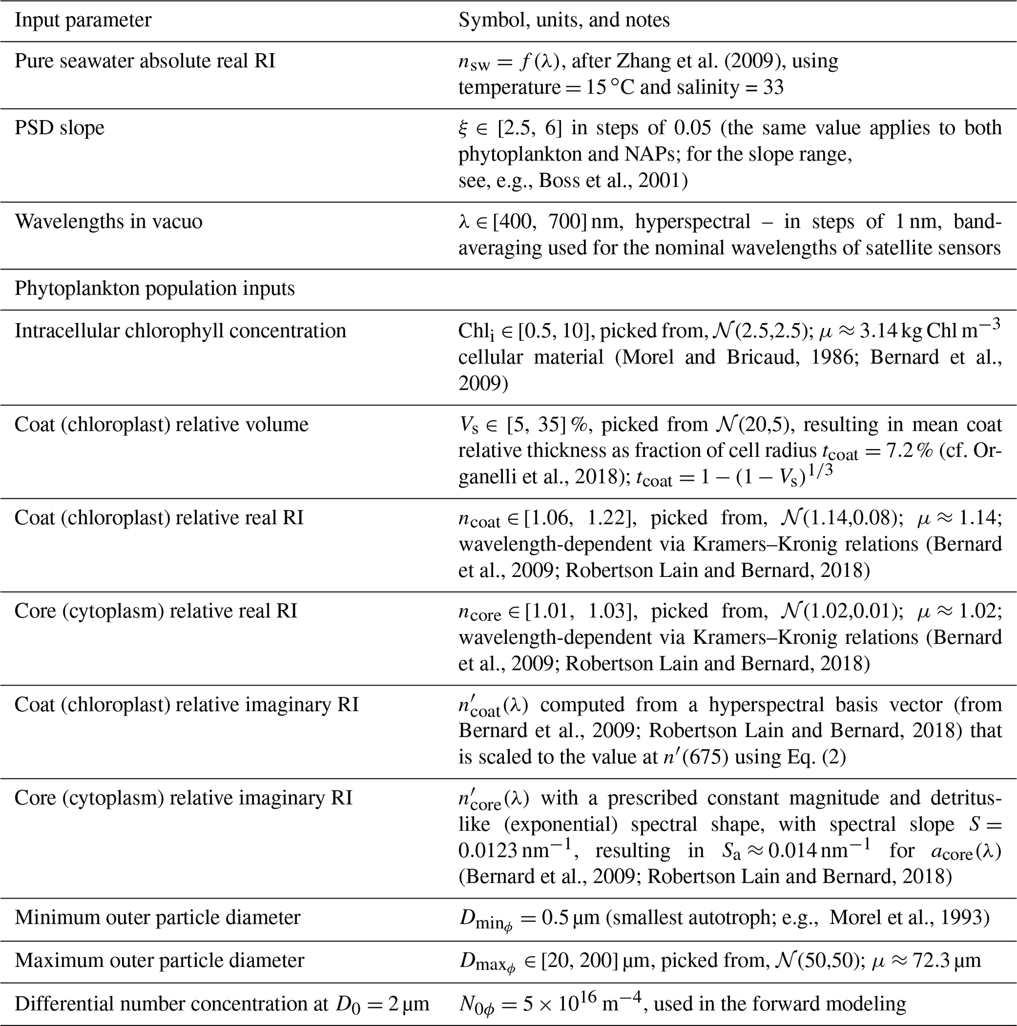
Table 2Inputs for the homogeneous-sphere Mie scattering code for the NAP population. Modeling inputs common to both phytoplankton and NAPs are given in the first three table rows of Table 1. 𝒩(μ,σ) stands for a normal distribution with mean μ and standard deviation σ.
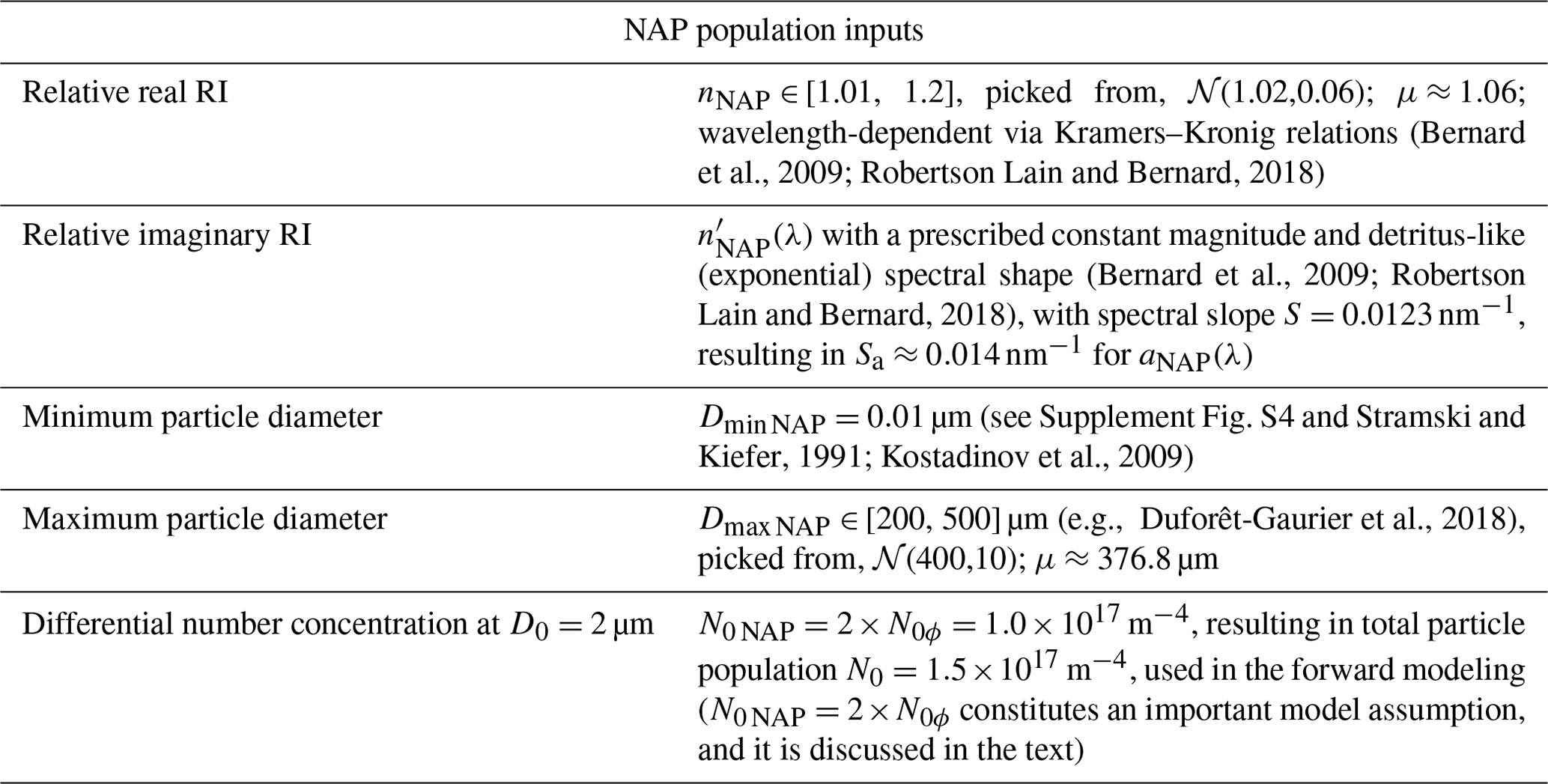
The NAP population is represented by a homogeneous sphere, the relative RIs of which are picked so that its absorption spectrum is detritus-like (same as the core of phytoplankton), and its real RI is allowed to vary over a wider range of values, meant to represent mostly organic detritus, but with some minerogenic contributions, resulting in a mean nominal relative real RI of ≈ 1.06. The input RIs and other input parameters for NAPs are summarized in Table 2.
Specification of the input PSD parameters and the relationship of NAPs to phytoplankton PSDs is key to the construction of the forward and inverse models. Necessarily, some key simplifying assumptions are made here in order to construct an algorithm with operational application to modern multispectral ocean color sensors. The two key assumptions are that (1) phytoplankton and NAPs have a power-law PSD (Eq. 1) with the same slope ξ, and (2) the scaling parameter N0 for NAPs is twice that of N0 for phytoplankton (the forward model uses default values as in Tables 1 and 2). The latter assumption is chosen so that it results in a phyto C : POC ratio of 1:3 (see Kostadinov et al., 2016a; Behrenfeld et al., 2005; and Sect. 3.4 here) (as long as they are both estimated using the same size ranges). Together, these assumptions allow for the retrieval of one common PSD parameter set pertaining to the total particle population PSD (one ξ value and one total N0 equal to the linear sum of the NAPs and phytoplankton N0 values).
2.2 Backscattering calculations
The backscattering efficiencies, Qbb(λ), for a single phytoplankton cell and a single non-algal particle were computed using the inputs described above in Sect. 2.1 and Tables 1 and 2. The coated-sphere code of Zhang et al. (2002) was used for both coated and homogeneous spheres. This code is included with the algorithm development scientific code of the PSD algorithm (see “Data availability”). Calculations were run for N=3000 instances of Monte Carlo simulations, each with a unique randomly picked combination of inputs for phytoplankton and NAPs. This resulted in 3000 sets of hyperspectral Qbb values. High sampling resolution in diameter space was picked for the coated spheres (10 000 samples between minimum and maximum diameter) in order to minimize the influence of resonance spikes in Qbb. For NAPs, 1000 samples of D were used.
Indices of refraction for both phytoplankton and NAPs are specified hyperspectrally (Supplement Fig. S1), and the computations are performed from 400 to 700 nm wavelength in vacuo with a step of 1 nm, allowing the resulting hyperspectral Qbb(λ) values to be adapted for use with any combination of visible optical wavebands pertaining to recent and currently operating ocean color multispectral sensors or for planned (e.g., PACE Werdell et al., 2019) or existing hyperspectral sensors.
Before bbp calculation, hyperspectral backscattering efficiencies, Qbb, for each Monte Carlo run were first pre-processed by applying quality control and band-averaging using a moving-average 11 nm wide top-hat filter (using as central wavelengths the nominal bands of the following ocean color sensors: Sea-viewing Wide Field-of-view Sensor, SeaWiFS; Moderate Resolution Imaging Spectroradiometer, MODIS, Aqua; Medium Resolution Imaging Spectrometer, MERIS, and Ocean and Land Colour Instrument, OLCI; and the Visible and Infrared Imager/Radiometer Suite, VIIRS, on the Suomi National Polar-orbiting Partnership, S-NPP, plus 440 and 550 nm), resulting in 19 unique bands for band-averaged backscattering efficiencies, denoted here as . The band-averaged spectral particulate backscattering coefficient, , was then calculated from the values and the input PSD as follows (e.g., van de Hulst, 1981; Kostadinov et al., 2009):
where m is the complex index of refraction (specified separately for coat and core in the case of phytoplankton). Equation (3) is applied separately to the modeled phytoplankton and NAP Qbb values and for each of the 3000 Monte Carlo runs. Band-averaged total spectra are then calculated as the linear sum of phytoplankton and NAP backscattering.
2.3 PSD retrieval via spectral angle mapping
2.3.1 End-member construction
Band-averaged total spectra were used to construct the backscattering end-members, , corresponding to specific input values of the PSD slope ξ. First, individual total bbp spectra from each Monte Carlo run (N=3000) were normalized by the value at 555 nm. The median of all normalized spectra at each waveband was used as the end-member for each PSD slope, from ξ=2.5 to ξ=6 in steps of 0.05 (see Table 1). This approach allows the isolation of the bbp spectral shape (dependent on ξ) and spectral magnitude (dependent on N0) (Eq. 3). Using the hyperspectral underlying Qbb values, end-members can be constructed for any desired set of wavelengths.
2.3.2 PSD parameter retrieval and operational application to OC-CCI ocean color data
The PSD parameters ξ and N0 are retrieved using the backscattering end-members, , via the spectral angle mapping (SAM) technique (e.g., Dennison et al., 2004). Briefly, the end-members and satellite-observed bbp spectra are treated as n-dimensional vectors, where n is the number of bands. The spectral angle between a given end-member and the observed spectrum is then calculated using the vector dot product as
Thus, spectral angle is an index of spectral shape similarity between two spectra, with more similar spectral shapes resulting in lower spectral angles. Equation (4) was used to calculate the spectral angle Θ between each of the 71 end-members, , and the input observed spectrum. The value of ξ corresponding to the smallest spectral angle is then assigned as the retrieved PSD slope. Three wavebands were used, namely 490, 510, and 550 nm. For operational application to OC-CCI v5.0 (Sathyendranath et al., 2021) remote-sensing reflectance (Rrs(λ)) data (which do not have the 550 nm band), band-shifting was applied to the input Rrs(560) to estimate the corresponding Rrs(550), which is used in the Loisel and Stramski (2000) IOP inversion. The band-shifting was constructed using the band ratios between the respective original and target bands from a hyperspectral run of the Morel and Maritorena (2001) (MM01) model. No other bands were shifted.
The N0 parameter is subsequently retrieved as the ratio of (1) the satellite-observed value of bbp(443) and (2) the median value of the quantity corresponding to the end-member class of the retrieved ξ and all statistically similar classes (see Supplement Sect. S1) across all Monte Carlo simulations.
2.4 Derived products: size-partitioned phytoplankton carbon, PSCs, POC, and chlorophyll
Once the PSD parameters are known, they can be used to compute derived products (Kostadinov et al., 2010, 2016a; Roy et al., 2017). Phytoplankton carbon in any size class spanning from cell diameter Dmin to cell diameter Dmax (m) can be estimated as
where , and N0 (m−4) for the total PSD is the satellite-retrieved parameter from total particulate backscattering; the other PSD parameters are as in Eq. (1). Equation (5) was used to compute size-partitioned phyto C in three size classes – picophytoplankton (0.2 to 2 µm in diameter), nanophytoplankton (2 to 20 µm in diameter), and microphytoplankton (20 to 50 µm in diameter) – as well as total phyto C as the sum of the three classes. Carbon-based PSCs are defined as the fractional contribution of each of the three size classes to total phyto C (Kostadinov et al., 2016a). Given the first-order correspondence between PSCs and PFTs (e.g., Le Quéré et al., 2005), these PSCs can also be interpreted as PFTs. The allometric coefficients of Roy et al. (2017) are used here, namely a=0.54 and b=0.85; when cell volume V is expressed in cubic micrometers, cellular carbon is computed in picograms of carbon per cell using these coefficients (Eq. 5; see also Menden-Deuer and Lessard, 2000). Phyto C in Eq. 5 is given in milligrams per cubic meter; the conversion factors in Eq. (5) are used to convert from cubic meters to cubic micrometers and from picograms to milligrams of carbon (Kostadinov et al., 2016a; Roy et al., 2017). The factor of is an assumption of the model (Tables 1 and 2). Thus, an estimate of POC (computed using the same size limits as total phyto C) was calculated as 3× phyto C.
Chlorophyll concentration was estimated from the PSD retrievals and the input intracellular chlorophyll concentration, Chli (Table 1; Roy et al., 2017), as follows:
In Eq. (6), Chli, D, D0, and N0ϕ all have to be expressed in consistent units so that Chl is obtained in milligrams per cubic meter. Here we use the median Chli across all Monte Carlo simulations to produce a single Chl estimate.
2.5 Validation and comparison
A data set of near-surface in situ PSD measurements was compiled for validation of the PSD parameter products, ξ and N0 (Eq. 1). The data set consists of Coulter counter and Laser In-Situ Scattering and Transmissometry (LISST) measurements and a small set of PSDs derived from multiple instruments and modeling. Specifically, the compilation consists of the following data sets: (1) a compilation of several data sets of Coulter counter measurements, as used in the KSM09 algorithm validation in Kostadinov et al. (2009); (2) LISST-100X (Sequoia Scientific©) measurements from the Plumes and Blooms project (e.g., Toole and Siegel, 2001; Kostadinov et al., 2007) in the Santa Barbara Channel, as used in Kostadinov et al. (2012); (3) Coulter counter measurements from the Atlantic Meridional Transect cruise no. 26 (AMT26) (Organelli and Dall'Olmo, 2018), as compiled and used in Organelli et al. (2018, 2020); (4) in-line LISST 100-X measurements from the cruises North Atlantic Aerosols and Marine Ecosystems Study 3 and 4 (NAAMES; https://science.larc.nasa.gov/NAAMES/, last access: 25 January 2023; Boss and Haëntjens, 2017) and EXport Processes in the Ocean from Remote Sensing (EXPORTS; https://oceanexports.org/, last access: 7 October 2022) North Pacific (NP) and North Atlantic (NA) (Boss and Haëntjens, 2018) (data were downloaded from the NASA SeaBASS database; Werdell et al., 2003); and (5) PSDs obtained using a volume scattering function (VSF) inversion technique (Zhang et al., 2011, 2012) from VSFs measured during the NASA EXPORTS campaign (Siegel et al., 2016) in the North Pacific in 2018 (Siegel et al., 2021).
The compiled PSD data set was used to fit for the PSD parameters of Eq. (1) using the 2 to 20 µm diameter range. One data point was removed from the 2018 EXPORTS PSD data due to a poor fit to a power-law PSD. These in situ estimates were matched to satellite OC-CCI v5.0 (Sathyendranath et al., 2019, 2021) Rrs using the same matching methods described below for POC and picophytoplankton carbon data. Matched reflectances were used as input to the novel PSD algorithm presented here. The in situ and satellite PSD parameters were then compared using a type II linear regression and several additional algorithm performance metrics (e.g., Seegers et al., 2018), details of which are given in the caption of Fig. 8.
A large compilation of in situ POC data was collected from various public databases and private contributors and was used here to perform match-ups with satellite OC-CCI v5.0 data. In addition to the POC data (1997–2012) used in Evers-King et al. (2017) for algorithm validation (N=3891), this study also incorporated recent in situ POC data (2013–2020) from the SeaWiFS Bio-optical Archive and Storage System archive (Werdell et al., 2003) (https://seabass.gsfc.nasa.gov/, last access: 1 May 2021). The daily, 4 km, sinusoidal projection OC-CCI v5.0 data (1997–2020) (Sathyendranath et al., 2019, 2021) were used to extract the closest central satellite pixels to the in situ data points. If the central satellite match-up pixels were valid, the surrounding eight pixels (a 3×3 pixel box) were also extracted to estimate the mean, median, and standard deviation of all OC-CCI variables. The match-up data points were then averaged with respect to depth (0 to 10 m), location, and date. Moreover, a number of uncertain match-up data points were removed, as described below. A total number of 6041 match-up data points were obtained and used for analysis. Here, the median satellite Rrs(λ) matched-up spectra were used to compute the satellite-retrieved POC data using the PSD-based algorithm.
The in situ picophytoplankton carbon data set compiled and used for algorithm inter-comparison as part of the ESA POCO project (Martínez-Vicente et al., 2017) was used here to generate match-ups with satellite OC-CCI v5.0 Rrs data for further validation. Match-ups were generated in the same way as described above for POC.
All in situ data described above were excluded from the validation if any of the following conditions were met: (1) average bathymetric depth from a ≈ 9 km buffer around the in situ sample location was less than or equal to 200 m, or any grid cell elevations in that buffer were 0 m or higher, using a downsampled, 4 km version of the NOAA ETOPO1 data set (https://www.ngdc.noaa.gov/mgg/global/, last access: 23 October 2015); (2) the in situ sample depth was 15 m or greater; or (3) there were three or fewer satellite pixels available to use in the match-up, as detailed above.
All duplicate in situ match-ups (in the sense of multiple in situ data points that are close in space and time and receiving the same satellite match-up) were combined into a single match-up point as follows: for the PSD, the medians of the PSD measurements from the NAAMES and EXPORTS cruises in each LISST size bin for such duplicates were used for the calculation of in situ PSD parameters (a large number of duplicates since the data are in-line); for the rest of the PSD data, the fit PSD parameters themselves were averaged (a small number of duplicates). For the POC (large number of duplicates) and picophytoplankton carbon data (small number of duplicates), the averages of the duplicate in situ data were used.
In addition to validation against in situ measurements of the PSD, POC, and picophytoplankton carbon, satellite chlorophyll a (Chl) retrievals (using the standard algorithm of OC-CCI v5.0 at the match-up points) were compared with Chl estimated using the PSD retrieval (Eq. 6). Finally, global algorithm retrievals of total phyto C for May 2015 (using OC-CCI v5.0 data as input) were also compared with two alternative methods of retrieving phyto C: (1) the Roy et al. (2017) algorithm and (2) the Graff et al. (2012, 2015) algorithm, as implemented by NASA's Ocean Biology Processing Group (OBPG). Modeling and processing of results presented here are done using the sinusoidal projection images; maps presented here are given in equidistant cylindrical projection (i.e., unprojected latitude/longitude).
3.1 Forward and inverse modeling
The first step in the algorithm development is the generation of 3000 Monte Carlo realizations of backscattering efficiencies as a function of particle diameter and wavelength, Qbb(D,λ). The important differences between backscattering efficiencies of homogeneous and coated particles is discussed in Supplement Sect. S2. Here, we continue the discussion with the resulting integrated backscattering spectra (Eq. 3). Hyperspectral bbp(λ) spectra modeled using a single forward optical model run are shown in Fig. 1. The computations use the median values of inputs varied in the Monte Carlo simulations (Tables 1 and 2). These normalized spectra illustrate the strong spectral shape dependence on the PSD slope ξ. Phytoplankton bbp spectral shapes are complex, with various peaks and troughs near the absorption peaks of chlorophyll, but are more linear in the 490 to 550 nm range, which is the one used for the multispectral operational PSD algorithm. Regardless, the SAM methodology of retrieval used here allows for any spectral shape and does not impose a power-law fit to the shape of bbp, as is done in KSM09 (Kostadinov et al., 2009) (see also Loisel et al., 2006). NAP backscattering exhibits smooth shapes due to the smooth shape of their absorption (Fig. 1b). Fundamentally, it is evident from Fig. 1a and b that the higher the PSD slope ξ, the steeper the bbp spectral shape becomes, with higher values in the blue, since smaller particles dominate the signal. This dependence is at the root of the principle of operation of the PSD algorithm. For completeness, corresponding absorption spectra are illustrated in Supplement Fig. S3.
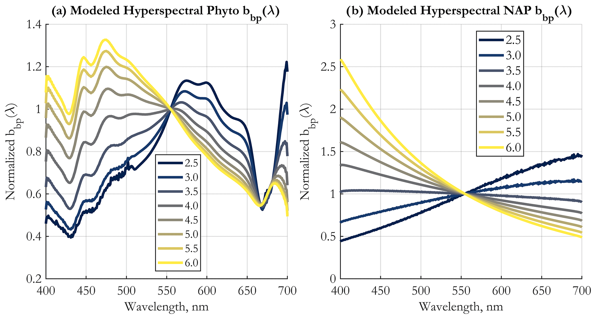
Figure 1Modeled hyperspectral backscattering coefficient of (a) phytoplankton, using EAP-based coated-sphere scattering computations, and (b) NAPs, modeled as homogeneous spheres, as a function of the input power-law PSD slope (color-coded solid lines, as in legend). All spectra are shown normalized to the respective values at 555 nm. See Sect. 2 for more details.
The 71 end-members (EMs) created for operational application to existing major satellite ocean color missions and corresponding to PSD slope values between 2.5 and 6.0 with a step of 0.05 are displayed in Fig. 2a. They represent the modeled spectra against which satellite-measured bbp spectra are compared using the SAM method (Eq. 4). The spectral shape dependence on ξ demonstrates the theoretical ability to retrieve this parameter from space.
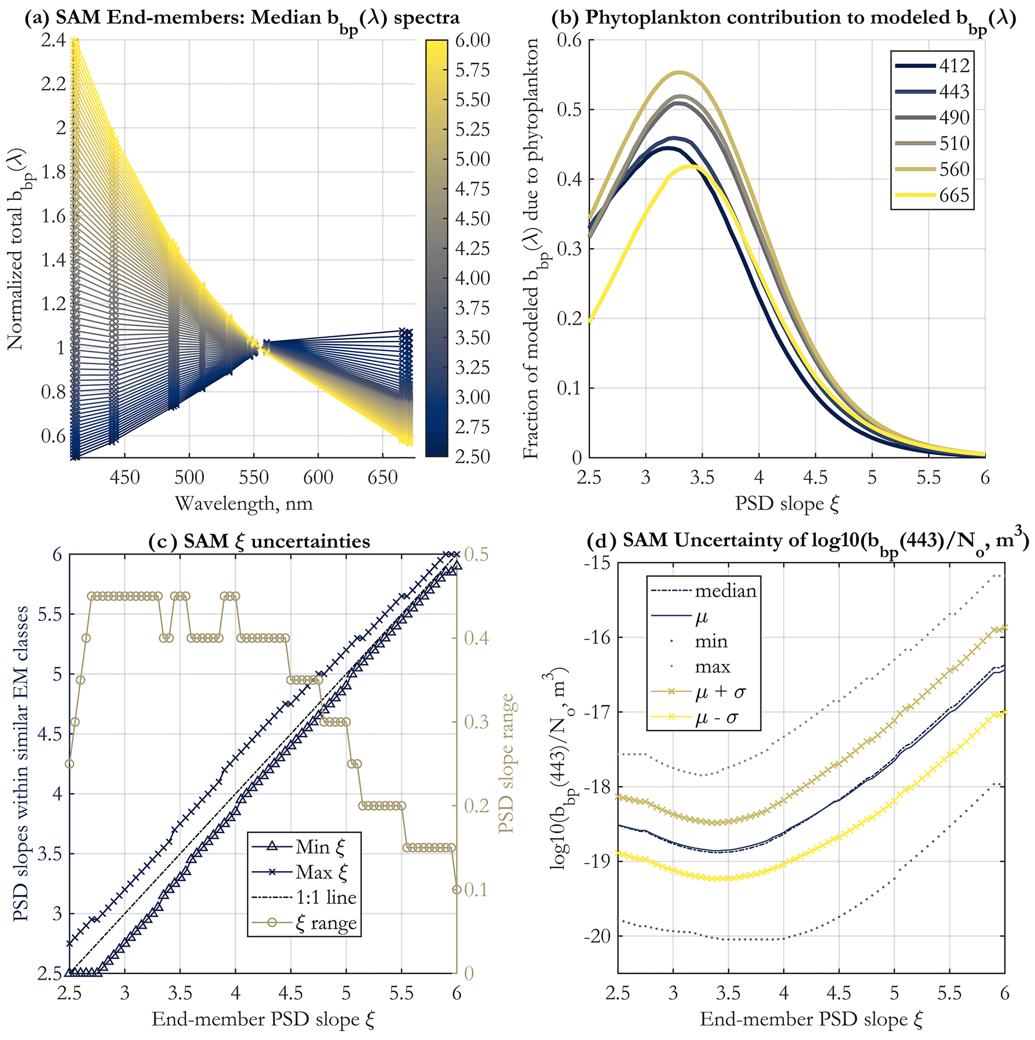
Figure 2(a) Normalized spectral shapes of the bbp end-members (EMs) developed for spectral angle mapping (SAM), shown at the 19 unique wavelengths used for band-averaging (see Sect. 2.2), and for PSD slopes as in the color legend. (b) The fraction of bbp(λ) due to phytoplankton as a function of the PSD slope ξ. The wavelengths shown are indicated in the legend (nm). The means across all 3000 Monte Carlo simulations are shown. (c) Uncertainties in the PSD slope ξ retrieval using the SAM method, for each EM. Shown are the minimum and maximum value of the PSD slope for all end-member classes that are statistically similar to the given EM, according to the Kruskal–Wallis ANOVA (Supplement Sect. S1) (left y axis), and the resulting range of PSD slopes (right y axis) falling within these asymmetric uncertainty bounds. (d) Statistics of the parameter for each EM, calculated for all 3000 Monte Carlo simulations and across all neighboring EM classes determined to be statistically similar to the given EM. μ in the legend stands for the mean, and σ is the standard deviation. The standard deviation of this parameter is used to estimate uncertainties in the N0 retrieval.
An important question in bio-optical oceanography is determining the sources of backscattering in the ocean and their relative contributions. This is still an unresolved issue (Stramski et al., 2004), though progress has been made (e.g., Organelli et al., 2018; Koestner et al., 2020; Zhang et al., 2020). This issue is of central importance to the PSD model, as it assigns varying fractions of the bbp signal to phytoplankton vs. NAPs under certain assumptions (Tables 1 and 2). Since in the two-component PSD model presented here phytoplankton and NAP bbp are modeled separately, the fraction of bbp due to phytoplankton vs. NAPs can be calculated. For a given PSD slope ξ and wavelength, the assumptions of the model dictate fixed fractional contributions by NAPs and phytoplankton to total bbp, which are given in Fig. 2b. There is variability by wavelength, but the first-order variability is driven by the PSD slope, namely at low ξ values (ξ<4.0), phytoplankton contribution to bbp is on the order of 30 % to 50 %, and it drops to near 0 % for higher slopes as ξ approaches 6.0. The curves are not monotonic, and peak phytoplankton contribution to bbp occurs at ξ≈3.25.
The fractional contributions of Fig. 2b are derived from the forward theoretical modeling, and they are influenced by all model assumptions and are not validated independently. In particular, the decisions on integration diameter limits for NAPs and phytoplankton, as well as on the distributions of the indices of refraction for phytoplankton and NAPs, will have a strong influence on these values. Since NAPs are permitted here to have higher RIs than RIs typical of organic detritus only, if NAPs were strongly dominated by or composed only of organic particles, then NAP contribution to bbp would be overestimated here. Of course these RIs are likely to be spatially and temporally variable, and the algorithm can be further improved by investigating and implementing such variability. Bellacicco et al. (2018) estimated global absolute bbp due to NAPs and its fractional contribution to total bbp using analysis of correlations with Chl. Qualitatively and to first order, their global pattern of percent bbp due to NAPs agrees with the model results reported here, i.e., low relative NAP contributions at high latitudes and in eutrophic areas and higher relative contributions in more oligotrophic areas such as the fringes of the subtropical gyres (they exclude the gyres from their analysis) (cf. their Fig. 2c and 2b here). Note that the Bellacicco et al. (2018) estimate pertains only to NAPs non-covarying with Chl, making comparison harder. Further investigation is warranted to more rigorously compare their product to the values implicit in the PSD algorithm described here. Apart from analyzing the relative contribution of phytoplankton vs. NAPs to total bbp, it is of interest to investigate the relative contributions of various size ranges to the modeled backscattering coefficient. This is illustrated in Supplement Fig. S4 and further discussed in Supplement Sect. S3.
The uncertainty in PSD slope retrieval is illustrated in Fig. 2c. These estimates are not symmetric about the ξ value and are derived via Kruskal–Wallis analysis of variance to determine class similarity (Supplement Sect. S1). As in KSM09, the general tendency is for the range of uncertainty in ξ to increase for lower PSD slopes, but it is always less than 0.5. The uncertainty in the ratio used to retrieve the N0 parameter is shown in Fig. 2d in log10 space. Mean and median values are similar, and the uncertainty about them does not vary much with PSD slope, also similarly to KSM09. The uncertainty in Fig. 2d at each ξ value includes all statistically similar classes of EMs.
3.2 Operational application of the PSD–phyto C algorithm to OC-CCI v5.0 merged satellite data
3.2.1 PSD parameters
The operational PSD algorithm presented here was applied to the monthly 4 km OC-CCI v5.0 Rrs(λ) data set (Sathyendranath et al., 2019, 2021). Both PSD parameters (ξ and N0; Eq. 1) and derived products were generated (Sect. 2.3 and 2.4). These data and their monthly and overall climatologies (and associated uncertainties) are made publicly available (see “Data availability”). Here, we use May 2015 data to illustrate and discuss the new algorithm.
The PSD slope map (Fig. 3a) reveals a global spatial pattern consistent with expectations and with KSM09; namely the subtropical oligotrophic gyres are characterized by high PSD slopes (relatively high numerical dominance of small particles), whereas more eutrophic areas such as coastal areas, equatorial upwelling zones, and high latitudes exhibit lower slopes (increasing relative abundance of larger particles). This is consistent with oligotrophic ocean ecosystems being dominated by picophytoplankton, whereas microphytoplankton contribute significantly to the phytoplankton assemblage in eutrophic areas and during blooms (e.g., Kostadinov et al., 2009; Kostadinov et al., 2010; and references therein). PSD slope values retrieved by the SAM-based algorithm span the full modeled range of . This is in contrast to KSM09, where values below 3.0 were not retrieved. The N0 PSD parameter (Eq. 1) is, as expected, higher in coastal, high-latitude, and eutrophic areas (indicating higher particle loads) and lower in the oligotrophic subtropical gyres (Fig. 3b). N0 varies over a few orders of magnitude. Note N0's units of m−4 (Eq. 1) and that care should be taken when comparing Eq. (1) and N0 to other formulations of the PSD, e.g., the k parameter in Roy et al. (2017), as these are related but not equivalent (see also Vidondo et al., 1997).
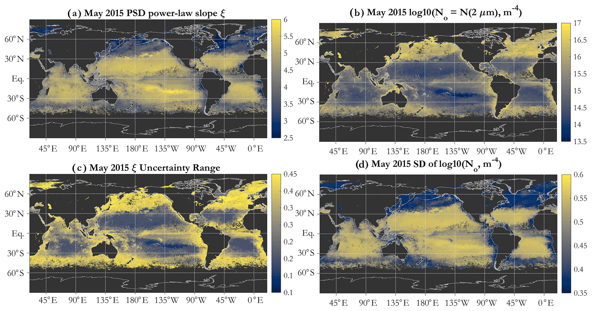
Figure 3Example operational retrievals of the PSD parameters (Eq. 1) and their uncertainties, using monthly OC-CCI v5.0 Rrs data for May 2015: (a) PSD slope ξ, (b) N0 parameter (m−4 in log10 space), (c) uncertainty range for ξ, and (d) standard deviation (SD) of log10 of N0.
Algorithm uncertainties are provided on a per-pixel basis. The uncertainty range estimates for ξ (Fig. 3c) (not necessarily symmetric about the ξ value) indicate that the gyres are characterized by lower uncertainties than the more eutrophic areas, as can be expected from Fig. 2c. These are partial uncertainty estimates, including those quantifiable and internal to the modeling, i.e., due to Mie parameter choices. Additional uncertainties inherent in the input OC-CCI Rrs values and those due to the IOP inversion algorithm used are not included in Fig. 3c and d and in subsequent propagated errors. Uncertainties in the N0 parameter are more uniform spatially but higher in the gyres (Fig. 3d). Note that those are given in log10 space as a standard deviation, and a relatively small absolute value of the uncertainty translates to relatively large uncertainties in absolute particle concentrations.
3.2.2 Phytoplankton carbon and carbon-based PSCs, POC, and chlorophyll from the PSD
Global patterns of total phytoplankton carbon (phyto C) retrieved via the PSD and allometric relationships (Fig. 4a) exhibit the expected lower values in the oligotrophic gyres and higher values elsewhere. Similarly to the results of Kostadinov et al. (2016a), values range over approximately 3 orders of magnitude, which is a higher range than retrievals based on other methods, namely direct empirical algorithm POC retrieval (Stramski et al., 2008) or the Behrenfeld et al. (2005) method of scaling backscattering, and it is also higher than the range in CMIP5 model ensembles (cf. Fig. 1 in Kostadinov et al., 2016a). This putative underestimation in the gyres and overestimation in eutrophic areas suggests the need for algorithm tuning, which is discussed in Sect. 3.3 along with implications of validation results. Global validation of phyto C retrievals with analytical phyto C measurements is planned but is currently challenging as phytoplankton-specific carbon data are relatively novel (Graff et al., 2012, 2015) and still scarce. Here, an initial validation effort is undertaken using several other variables; see Sect. 3.3.
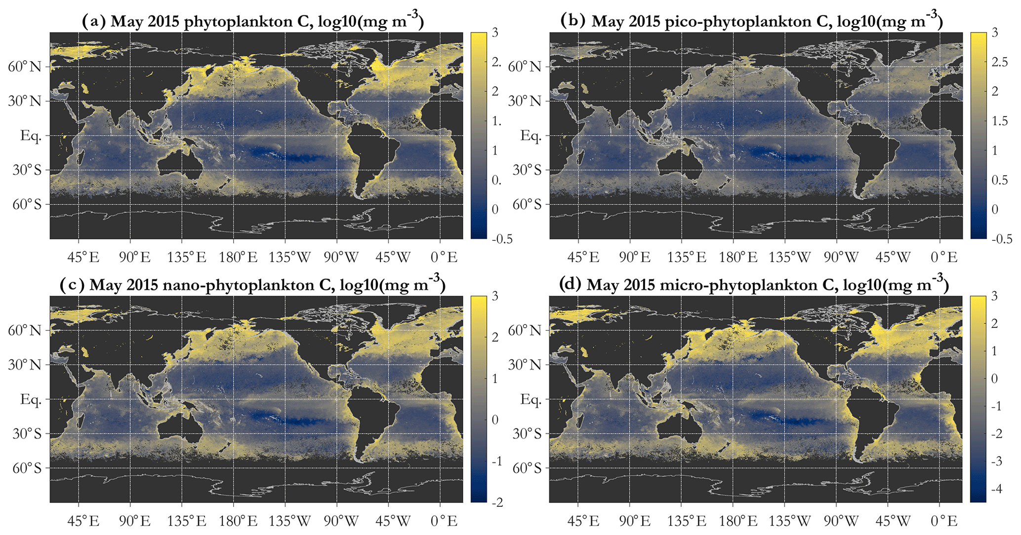
Figure 4Example operational PSD-based retrievals of total and size-partitioned phytoplankton carbon, using monthly OC-CCI v5.0 Rrs data for May 2015: total phytoplankton carbon (a), picophytoplankton carbon (b), nanophytoplankton carbon (c), and microphytoplankton carbon (d). Units are milligrams per cubic meter, mapped in log10 space. The diameter limits for the three size classes are picophytoplankton (0.2 to 2 µm), nanophytoplankton (2 to 20 µm), and microphytoplankton (20 to 50 µm).
A key feature of the PSD-based algorithm is that phyto C can be partitioned into any number of size classes by choosing appropriate integration limits of Eq. (5). Absolute concentrations of pico-, nano-, and microphytoplankton are illustrated for May 2015 in Fig. 4b, c, and d, respectively. Picophytoplankton C is mapped on the same color scale as total phyto C (Fig. 4a), but pico- and nanophytoplankton C maps have differing scales, illustrating that while picophytoplankton C varies over ≈ 3 orders of magnitude spatially and globally, nanophytoplankton C varies over ≈ 4–5 orders of magnitude, and microphytoplankton varies over ≈ 7 orders of magnitude (see also Kostadinov et al., 2010; Kostadinov et al., 2016a). Note that empirical tuning will affect these ranges of variability; see Sect. 3.3. Fractional contributions of each of the three PSCs used here to total phyto C are illustrated in Fig. 5. Picophytoplankton dominate much of the open-ocean, lower-latitude, oligotrophic areas, contributing nearly 100 % of the carbon biomass there (Fig. 5a); nanophytoplankton (Fig. 5b) contribute up to ≈ 50 % of the biomass in the higher-latitude and more eutrophic areas; and microphytoplankton (Fig. 5c) contribute significantly only in the most eutrophic areas, e.g., during the North Atlantic bloom at ≈ 45–50∘ N (May 2015 is shown). As previously noted (Kostadinov et al., 2010, 2016a), this general pattern is consistent with current understanding of ocean ecosystems.
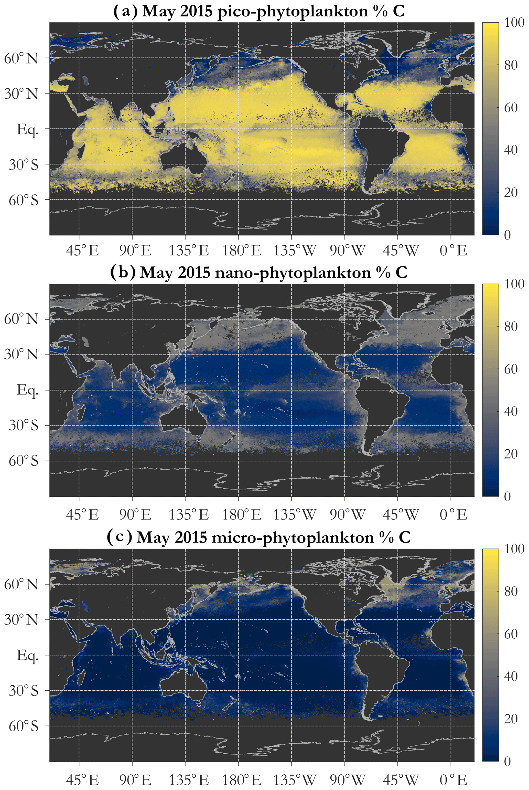
Figure 5Example operational retrieval of the percent contribution of each phytoplankton size class (PSC) to total phytoplankton carbon, determined via the PSD (Sect. 2.4). Retrievals use monthly OC-CCI v5.0 Rrs data for May 2015. The PSCs are picophytoplankton (a), nanophytoplankton (b), and microphytoplankton (c).
The fractional carbon-based PSCs (Fig. 5) are ratios of two integrals of Eq. (5); thus they are analytical functions of the PSD slope ξ and the b allometric coefficient (as well as the limits of integration used for each class and total phyto C). These functions are plotted in Fig. 6, together with the satellite-observed ξ histogram for May 2015, illustrating the most common values for the PSCs found in the ocean. Area-wise, the ocean is dominated by oligotrophic regions with high picophytoplankton contributions to C biomass.
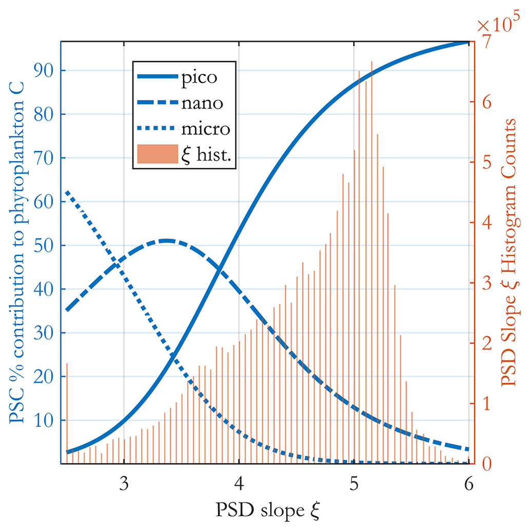
Figure 6Percent contribution of each PSC to total phytoplankton carbon (blue curves as in legend, left y axis) as a function of the PSD slope ξ. A histogram of the PSD slope from the (sinusoidal projection) OC-CCI v5.0-based image for May 2015 is shown in the background as brown bars (right y axis). The three PSC curves are analytically derived from the model, and no satellite data are used in producing them.
As an illustration of uncertainty propagation to derived products, the propagated uncertainty in total phyto C (Fig. 7a) and fractional picophytoplankton C biomass (Fig. 7b) is shown. Comparison of Fig. 4a with Fig. 7a indicates that absolute total phyto C uncertainties are of the same order of magnitude as the values themselves. This is a partial uncertainty estimation due to the assumed distributions of the Mie inputs (Tables 1 and 2) and due to the allometric coefficients. The Mie inputs are varied over wide ranges to accommodate various environments in the global ocean, with the goal of having a single first-principles-based operational algorithm applicable to first order globally. This increases the uncertainty estimates. The uncertainty for the fractional PSC products depends only on the uncertainties in ξ and b; thus they exhibit much lower internal algorithm uncertainty compared with absolute values. For picophytoplankton, they are % for the oligotrophic gyres and do not exceed ≈ 7 % globally. This suggests that the fractional PSCs are more reliable products than the absolute values, and they can also be used with other products to partition them, e.g., total phytoplankton carbon estimated using the alternative methods shown in Fig. 9 (namely Graff et al., 2015, and Roy et al., 2017) or the Behrenfeld et al. (2005) or Sathyendranath et al. (2020) methods; POC products (e.g., Stramski et al., 2008) can be partitioned this way as well. Per-pixel uncertainties are estimated for all products and composite imagery (climatologies) as well and are provided with the OC-CCI-based data set associated with this paper (“Data availability”).
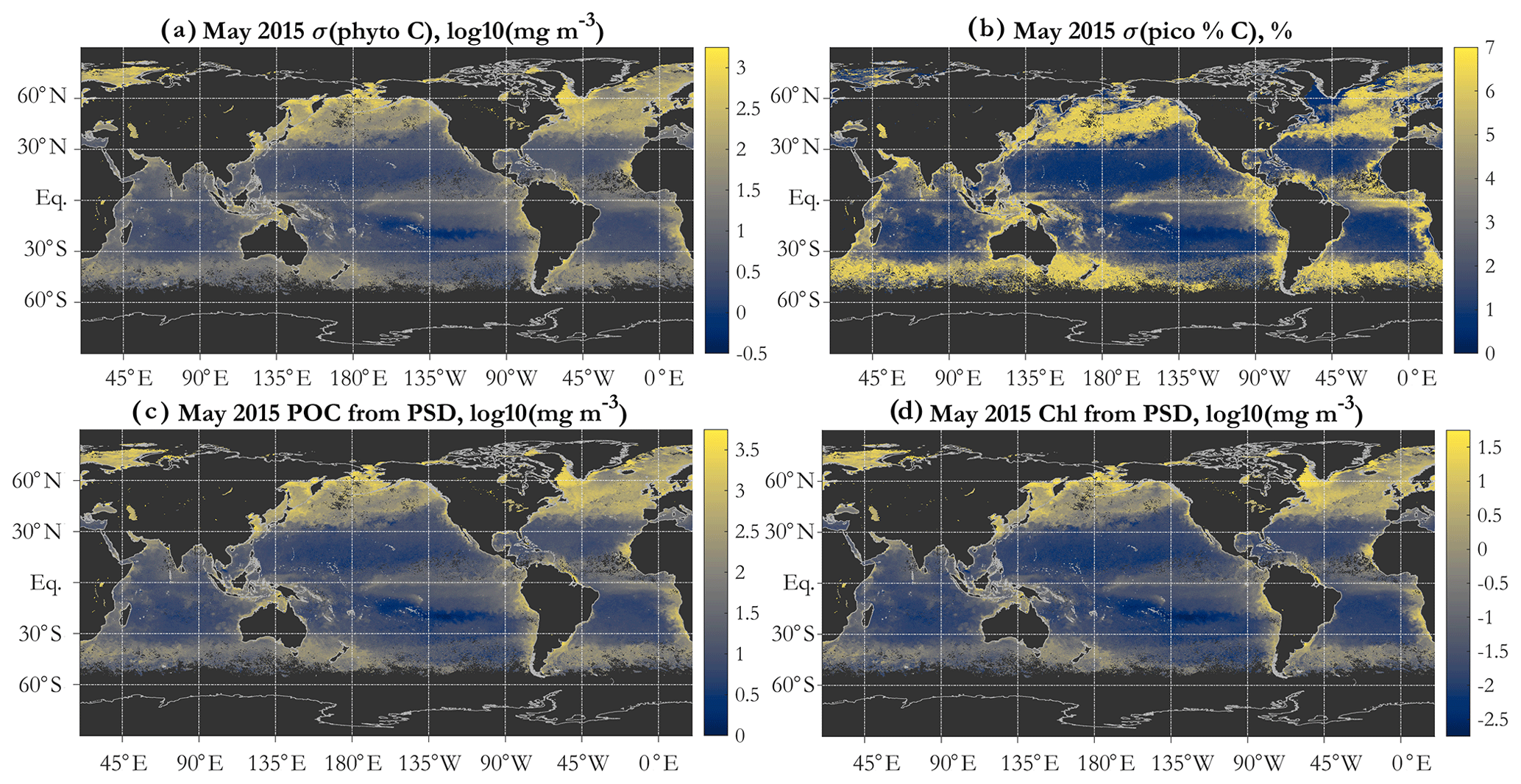
Figure 7Propagated uncertainty in (a) total phytoplankton carbon given as 1 standard deviation (in milligrams per cubic meter), mapped in log10 space, and (b) fractional contribution of picophytoplankton to total phytoplankton carbon, given as 1 standard deviation in percent. (c) POC derived using the PSD retrievals (in milligrams per cubic meter), mapped in log10 space, and (d) chlorophyll concentration (Chl) derived using the PSD retrievals (in milligrams per cubic meter), mapped in log10 space. Monthly OC-CCI v5.0-based data for May 2015 are shown in all panels.
The formulation of the PSD algorithm allows for both POC and Chl (Eq. 6) to be estimated from the retrieved PSD. Due to the assumptions used, POC is phyto C multiplied by 3 (Fig. 7c). This is strictly true only if the POC estimate uses the same limits of integration as phyto C, which is an approximation of the usual POC operational definition (see, e.g., discussion of POC–PSD closure analysis in Kostadinov et al., 2016a). POC is thus estimated to first order, treating the retrieved NAPs as being composed of POC only and applying the same allometric relationship to NAPs as to phyto C, in spite of the fact that the assumed RI distribution of the NAPs is broader (Table 2). These are simplifying assumptions of the two-component model; a more accurate POC representation can be achieved if organic and inorganic NAPs are modeled as separate particle populations (e.g., Duforêt-Gaurier et al., 2018). This is a planned development of the model in the future; the goal here is to build an operational PSD–phyto C algorithm (based on first principles, as mechanistic as feasible) for use with multispectral satellite data of limited degrees of freedom. Hyperspectral sensors such as PACE (Werdell et al., 2019) should allow for some more degrees of freedom and thus for more independent particle components and their PSDs to be modeled separately. However, note that even hyperspectral data have limits on their degrees of freedom, which are expected to be much fewer than the number of sensor bands (Lee et al., 2007; Cael et al., 2020). An important benefit of POC is that it is a widely observed variable, available for global validation efforts (Sect. 3.3), as is Chl. Similarly to POC, there are benefits of the PSD-derived estimate of Chl (Fig. 7d); it can be used as additional verification/validation of model retrievals, and/or PSD-retrieved Chl can be used as a parameter to optimize (in algorithm tuning), as discussed shortly (Sect. 3.3). Next, we discuss validation/verification and tuning efforts in which both PSD-derived POC and PSD-derived Chl are used.

Figure 8(a) Comparison of PSD slope derived from in situ measurements with the matched-up satellite retrieval (Sect. 2.5). Points are color-coded according to the corresponding matched-up satellite OC-CCI v5.0 Chl (colormap in milligrams per cubic meter in log10 space). In this figure (as well as in Figs. 10 and 11 and Supplement Figs. S6, S9, and S10), type II (reduced major axis, RMA) regression is used, and regression and validation statistics are given in the figure panels; “y-int” stands for the y intercept, RMS is root mean square (square root of the mean of squared differences between the in situ and satellite values), bias is the mean of the satellite minus in situ values, and MAE is the mean absolute error (the mean of the absolute values of the differences between the in situ and satellite values) (e.g., Seegers et al., 2018). The values in parentheses are the standard deviations of the slope and y intercept, respectively. (b) Same as in panel (a) for the N0 parameter (Eq. 1) (axes in log10 space).
3.3 Algorithm validation, comparisons, and empirical tuning for the N0 PSD parameter and absolute concentrations
In an initial validation effort, the novel PSD–phyto C algorithm is validated/verified using several variables. It is challenging to globally and thoroughly directly validate the major products of the algorithm – the PSD and size-partitioned phyto C – due to a paucity of globally spanning in situ observations, which are further reduced when performing satellite match-ups. Here, we validate or verify algorithm performance against compilations of the following variables: (1) in situ PSD observations (Sect. 2.5), (2) in situ POC observations, (3) in situ picophytoplankton C observations, and (4) concurrent satellite observations of Chl. Maps of the locations of in situ observations are shown in Supplement Fig. S5. In addition, we compare phyto C retrievals to several existing methods using the example May 2015 OC-CCI v5.0 image. Further, based on these results, we suggest an empirical tuning of the algorithm.
Validation results for the PSD slope ξ (Fig. 8a) indicate a statistically significant but noisy relationship between retrieved and observed slopes, with a positive bias for satellite retrievals and a regression slope substantially greater than unity. Most validation points are scattered in a cloud of data between 3.0 and 4.5 and do not exhibit much correlation, and there is a somewhat separate cluster of data centered about a slope of 5.25 in the satellite retrieval that have smaller corresponding in situ values of about 4.0. There is generally a clear tendency for points from more oligotrophic areas (as indicated by Chl color coding) to exhibit higher satellite values and more eutrophic areas to exhibit much lower satellite values. This tendency is weaker for the in situ observations, which tend to have a narrower range, mostly between 3.0 and 4.5. To first order, the satellite data are in the same range as in situ data, and the retrievals capture the in situ data trend; however, there is a pattern of having a bigger range of PSD slopes in satellite data than in the in situ match-ups, with the algorithm underestimating low values and overestimating high values.
Validation for the N0 parameter (Fig. 8b) is statistically significant (somewhat higher R2 than the ξ regression) but also quite noisy. Strong clustering of the in situ observations around 1015.5–1016.0 m−4 is observed, and the majority of these observations are somewhat overestimated in the satellite retrievals, which cluster around 1016.25. Notably, a separate cluster associated with low Chl (and low values of both satellite and in situ N0) shows that the satellite retrievals substantially underestimate these field data. Since N0 is the PSD scaling parameter, which generally controls absolute number, volume, and carbon concentration variability to first order, this has implications for the global pattern of phytoplankton carbon retrievals (Fig. 4); namely it is consistent with underestimation in the oligotrophic gyres and overestimation in the eutrophic areas. Overall, both satellite and in situ data exhibit increasing values of N0 with increasing Chl concentrations, as expected; i.e., more oligotrophic waters are associated with smaller overall particle number concentrations. Further discussion of the PSD validation by location of in situ data (Fig. S5a and b) is provided in Supplement Sect. S4 and illustrated in Supplement Fig. S6.
This pattern of under- and overestimation in the N0 validation drives the slope of the validation regression to be much greater than unity and suggests an empirical tuning to absolute phytoplankton carbon estimates via a linear (in log10 space) tuning of N0, as done in TK16 (Kostadinov et al., 2016a), who based the tuning on the validation regression. A similar approach is proposed here, but it is derived differently. Details of the tuning derivation procedure are given in Supplement Sect. S5. The following global tuning equation was obtained:
where N0 is the original (untuned) PSD parameter. This tuning changes N0 retrievals in a similar fashion to the TK16 tuning and is consistent with a tuning suggested by the N0 in situ validation presented here (Fig. 8b); namely, low satellite N0 values are increased, and high N0 values are decreased, narrowing the overall range of variability of retrieved N0 and thus the range of the retrieved derived variables. This addresses the low bias in oligotrophic gyres and the high bias in eutrophic areas. The goal of the tuning is to get more realistic absolute retrievals of POC and Chl (hypothesizing that this should also lead to more realistic phyto C retrievals; however, see discussion about picophytoplankton validation in Sect. 3.3.2).
The tuned N0 parameter for May 2015 is mapped in Supplement Fig. S7a. The overall spatial pattern of higher values in more eutrophic areas is preserved, but the global range of values is reduced compared to the original formulation, increasing N0 in the gyres and decreasing it in more productive areas. The resulting multiplicative factor to be applied in linear space to phyto C, POC, and Chl values is mapped in log10 space in Supplement Fig. S7b. Values in oligotrophic areas are generally greater than unity in linear space (mostly between 1 and 10), indicating that the tuning increases phyto C, POC, and Chl in these areas, up to about an order of magnitude (in limited areas mostly in the South Pacific Gyre) and more moderately elsewhere in the tropical and subtropical oligotrophic oceans. The equatorial upwelling areas and other transitional zones are not changed, and high-latitude oceans exhibit correction factors mostly less than unity in linear space (mostly between 0.1 and 1), which decreases phyto C and Chl up to an order of magnitude (rare, mostly less). This tuning is not applied to figures previously discussed here.
3.3.1 Comparison of the PSD-based phytoplankton carbon retrieval with existing satellite algorithms
In this section, we compare PSD-based phyto C retrievals presented here with two existing methods for its retrieval. The May 2015 original total phyto C retrieval is compared with the tuned total phyto C and the retrievals of the absorption- and PSD-based algorithm of Roy et al. (2017) and with the Graff et al. (2015) algorithm in Supplement Fig. S8. The histograms of these four images are compared in Fig. 9. The tuned retrievals are similar to those of Graff et al. (2015), whereas the original retrievals are similar to those of Roy et al. (2017), and the latter two have wider ranges globally compared to the former two. Of these algorithms, the simplest is that of Graff et al. (2015), as it is a direct scaling of bbp, and it is based on in situ chemical analytical measurements of phyto C (Graff et al., 2012, 2015). These dichotomous inter-comparison results suggest that further algorithm inter-comparison and validation with direct in situ measurements of phyto C are needed to guide future algorithm developments; however these data are relatively novel and scarce globally. Validation results using in situ POC and picophytoplankton carbon (discussed next) exhibit a similar dichotomy.
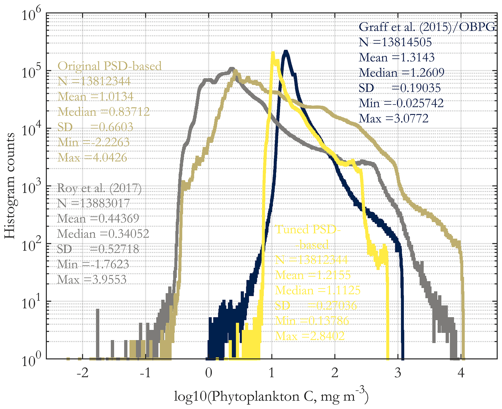
Figure 9Histograms of the images of Supplement Fig. S8, including the original PSD-based phyto C retrieval (Fig. 4a). Histogram counts are given on a log10 scale on the y axis, and the variable (x axis) is log-transformed as well. All four histograms are derived from the sinusoidal projection images for May 2015, using monthly OC-CCI v5.0 data.
3.3.2 Validation using POC and picophytoplankton carbon in situ data
PSD-based estimates of POC are validated against in situ measurements for the original algorithm (Fig. 10a) and the tuned algorithm (Fig. 10c). Both regressions have satisfactory R2 values and also illustrate that in general higher POC values are associated with higher Chl (colormap). Notably, the original algorithm validation has a slope of ≈ 2 and exhibits substantial underestimates at low POC and overestimates at high POC. As intended, the tuning corrects this range exaggeration and significantly improves the slope, intercept, bias, RMS, and MAE. The regression with the N0 tuning applied should not be considered a truly independent validation because the algorithm has been empirically tuned to retrieve POC well; however, the tuning was done with global POC imagery (using monthly images for 2004 and 2015) that uses the Stramski et al. (2008) empirical POC algorithm, not with these in situ POC data directly.
In addition to the validation with in situ POC, we performed a comparison of the matched satellite Chl and the corresponding PSD-based Chl estimate (Eq. 6) for the original (Fig. 10b) and the tuned algorithm (Fig. 10d). Both comparisons exhibit very high R2 values, and similarly to POC, the original algorithm underestimated Chl at low values and overestimated Chl at high values. The tuning successfully addresses this, leading to excellent overall comparison of the tuned algorithm, with a slope near 1.0 and a low intercept. However, for the lowest Chl values (Chl <0.1 mg m−3), performance deteriorates. The tuned comparison is not a fully independent validation, as the algorithm was tuned to compare well with OC-CCIv5.0 satellite retrievals (using global monthly images for 2004 and 2015). Overall, the comparison with Chl is encouraging, indicating that the model is able to reasonably reproduce (with tuning) OC-CCI v5.0 standard satellite Chl values at the match-up points.
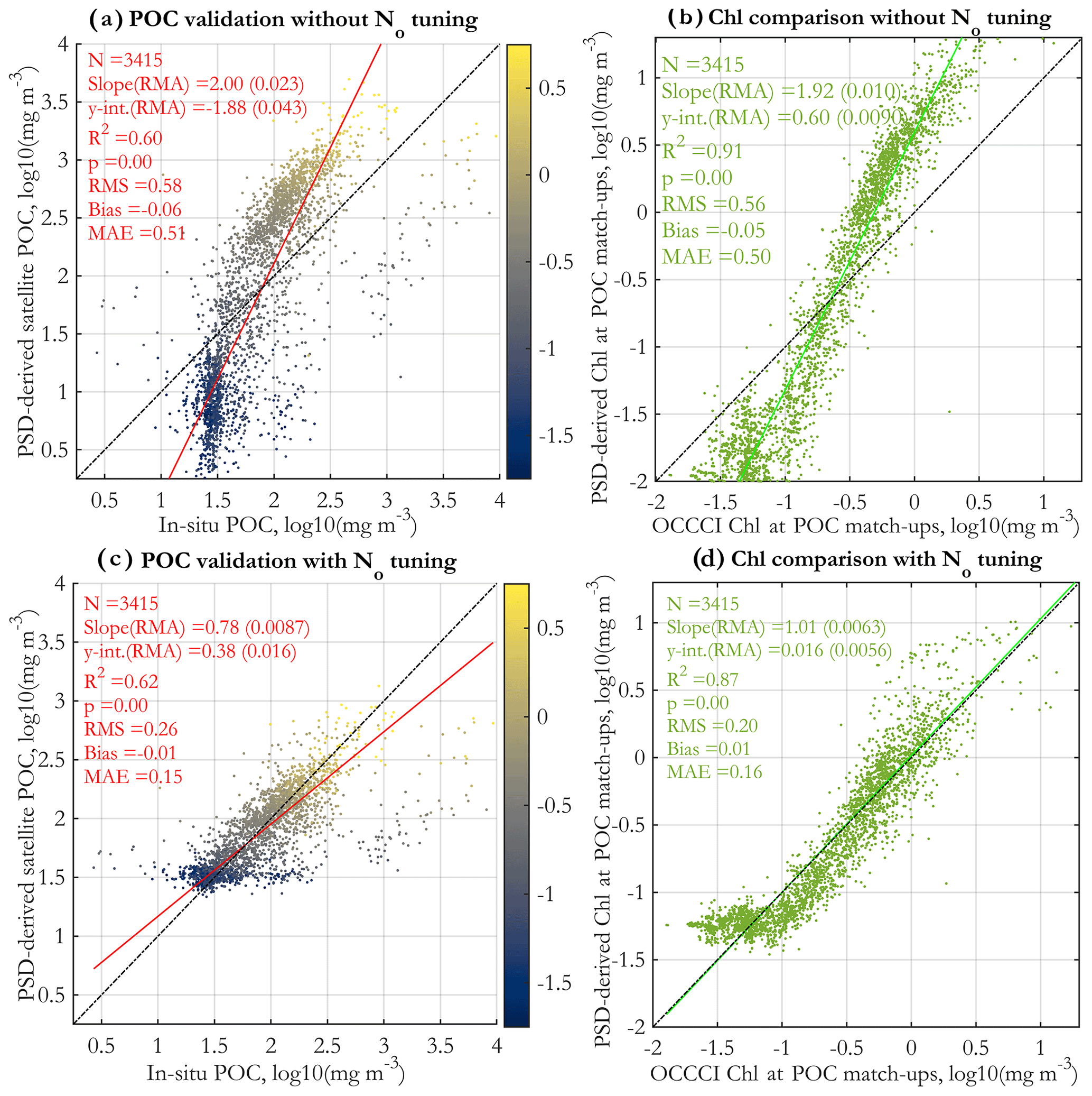
Figure 10Validation of PSD-based POC retrievals vs. in situ POC measurements (a, c) and comparison of satellite retrievals of Chl using the standard OC-CCI v5.0 algorithm vs. Chl estimated from the PSD (b, d). Panels (a) and (b) have no tuning applied, whereas empirical tuning is applied to the N0 parameter (Eq. 7) for panels (c) and (d). The tuning procedure applies a linear correction to N0 in log10 space to ensure reasonable retrievals of POC and Chl, based on monthly satellite images from 2004 and 2015; for details, see Supplement Sect. S5. The data points in panels (a) and (c) are colored by their matched standard OC-CCI v5.0 satellite Chl values (colormap, in milligrams per cubic meter in log10 space).
Validation against in situ picophytoplankton carbon is presented in Fig. 11a (with no N0 tuning applied) and in Fig. 11c with the tuning applied. The corresponding Chl comparisons between matched standard OC-CCIv5.0 Chl and Chl derived via the PSD model are shown in Fig. 11b and d. As with the POC match-ups (Fig. 10b and d), comparisons with Chl are better for the tuned version of the algorithm, indicating that the tuning is needed to reproduce more realistic Chl values globally. However, the tuning does not lead to any improvement in the validation results of picophytoplankton C (cf. Fig. 11a and c). The validation regression without tuning is statistically significant (p<0.05), albeit noisy (low R2=0.18); satellite retrievals and in situ data cover approximately the same ranges, and increasing Chl and in situ picophytoplankton C generally correspond to increasing satellite values as well, with some tendency for under- and overestimation as with the other variables. However, the tuned satellite retrievals have a very narrow range that does not cover the range of the in situ data, and validation statistics are generally worse than those of the original validation (the regression is not significant at the p=0.05 level). These validation results are generally consistent with the results of Martínez-Vicente et al. (2017), where the tuned version of the TK16 (Kostadinov et al., 2016a) algorithm was used.
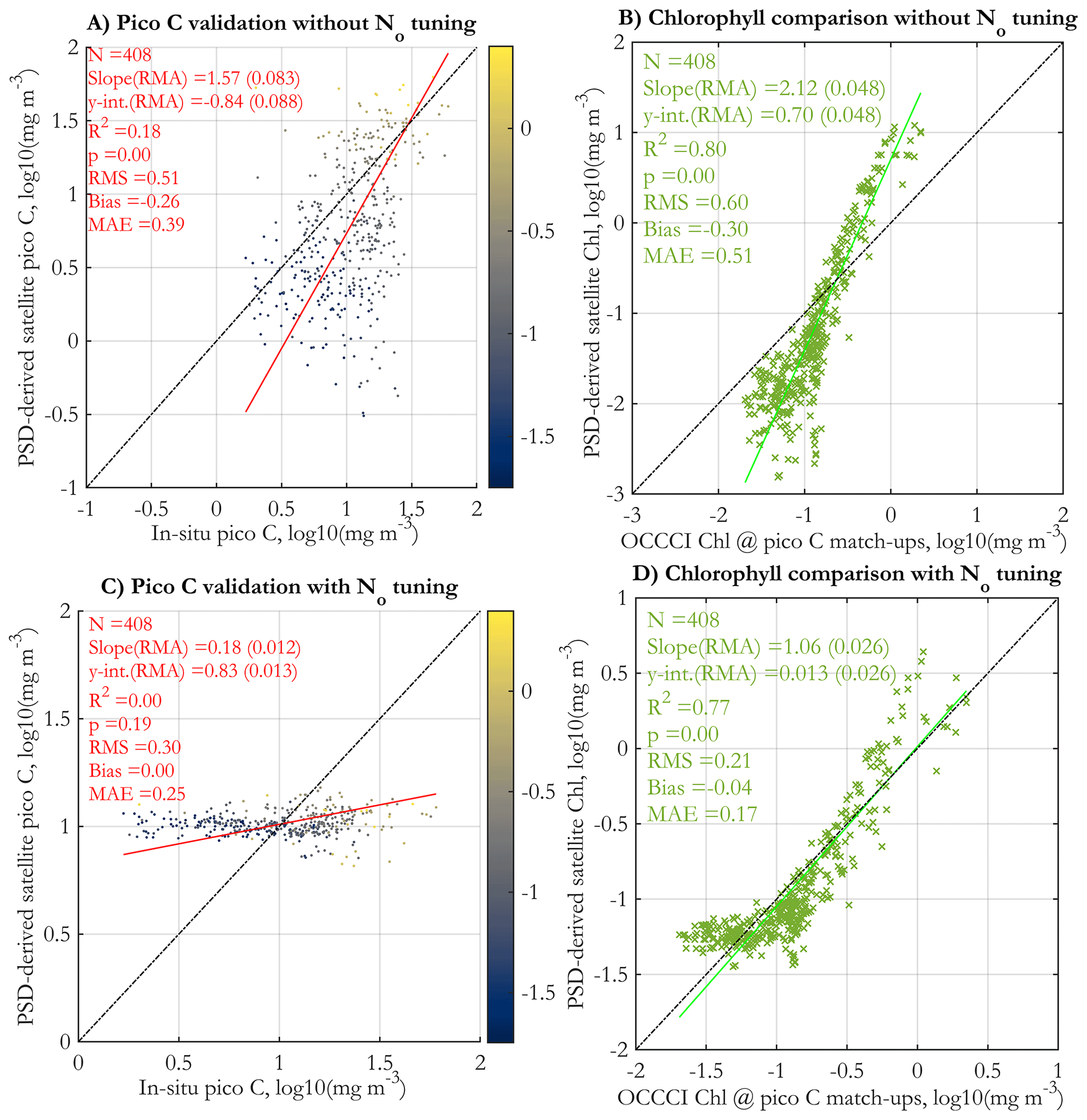
Figure 11Validation of picophytoplankton carbon derived from the PSD model using daily OC-CCI v5.0 satellite data vs. in situ measurements, as used in the POCO project (Martínez-Vicente et al., 2017) (a, c). Comparison of PSD-derived satellite Chl (y axes) with the matched satellite retrieval of Chl using the standard OC-CCI v5.0 algorithm at the locations of the in situ picophytoplankton carbon match-up points (x axes) (b, d). Panels (a) and (b) have no tuning applied, whereas empirical tuning is applied to the N0 parameter (Eq. 7) for panels (c) and (d). The tuning procedure applies a linear correction to N0 in log10 space to ensure reasonable retrievals of POC and Chl, based on monthly satellite images from 2004 and 2015; for details, see Supplement Sect. S5. The data points in panels (a) and (c) are colored by their matched standard OC-CCI v5.0 satellite Chl values (colormap, in milligrams per cubic meter in log10 space).
3.4 Further discussion, summary, and conclusions
The novel PSD–phyto C algorithm described here represents a major overhaul of the KSM09 algorithm (Kostadinov et al., 2009) (a comparison between KSM09 and the present algorithm is briefly discussed in Supplement Sect. S6). Unlike KSM09, two distinct particle populations are used: phytoplankton and NAPs. Phytoplankton backscattering is modeled using coated-sphere Mie calculations with inputs based on the Equivalent Algal Populations (EAP) approach (Bernard et al., 2009; Robertson Lain and Bernard, 2018). This model formulation allows assessment of the percent contribution of phytoplankton and NAPs to total bbp as well as the estimation of Chl from the retrieved PSD. Underlying bbp forward modeling is hyperspectral, facilitating adaptation of the algorithm to upcoming hyperspectral sensors like PACE (Werdell et al., 2019). PSD retrieval is achieved via spectral angle mapping (SAM), and no spectral shape is imposed on bbp; operational end-members for current and past multispectral sensors and the OC-CCI v5.0 merged ocean color data set are created via band-averaging from the underlying hyperspectral modeled bbp.
The algorithm has been used to create an accompanying data set based on the OC-CCI v5.0 data set (Kostadinov et al., 2022b; see “Data availability”). We emphasize that the PSD parameters and derived retrievals presented here and in the accompanying data set (Kostadinov et al., 2022b) are an experimental research satellite product with relatively large uncertainties. We do not claim that it is akin in validity and accuracy to the more established (and much more empirical!) algorithms for canonical products such as Chl and POC. As emphasized elsewhere in this text, the goal is to build an operational algorithm based on first principles as much as feasible, even at the expense of accuracy, in order to push the boundaries of what is retrievable from space and move the science of bio-optical algorithm development forward. Potential users of these PSD and derived data (Kostadinov et al., 2022b) need to be aware of their limitations, uncertainties, and validation status before using them, for example, in building or validating/constraining biogeochemical models. The choice of IOP algorithm to retrieve bbp(λ) is key for the PSD–phyto C algorithm, as the spectral shape of bbp is what the PSD slope retrieval is based upon (Eq. 4). The Loisel and Stramski (2000) IOP algorithm is chosen here, as in KSM09, because it allows spectral bbp retrievals that are not constrained by a specific spectral function or parameterization of bbp as is done, for example, in the QAA (quasi-analytical algorithm; Lee et al., 2002) and the GSM (Garver–Siegel–Maritorena) algorithm (Maritorena et al., 2002, 2010). For the wavelengths used in the PSD slope retrieval, modeled and satellite-derived bbp spectral shapes compare well when the Loisel and Stramski (2000) algorithm is used, and global patterns of the retrieved PSD parameters appear reasonable. Preliminary tests with Loisel et al. (2018) indicate that this algorithm is not as suitable for PSD retrieval in this regard. Use of Loisel et al. (2018), Jorge et al. (2021), and other IOP algorithms will be further investigated in future development of the PSD algorithm.
An important assumption of the model is that N0 for NAPs is twice that for phytoplankton so that the phyto-C-to-POC ratio is a constant 1:3. This ratio is expected to vary in the real ocean, and the value used here is a reasonable average choice (e.g., Behrenfeld et al., 2005; Jackson et al., 2017; Thomalla et al., 2017; and references therein). Graff et al. (2015) employed the cell sorting and chemical analysis methods of Graff et al. (2012) to measure phyto C in the equatorial Pacific and along the Atlantic Meridional Transect (AMT). Their results indicate that a phyto C : POC value of 1:3 is reasonable, falling within their observed ranges; however, they do observe many higher values, particularly in the oligotrophic gyres. The ratio of Roy et al. (2017) phyto C to Stramski et al. (2008) POC (applied to the May 2015 monthly image of the OC-CCI v5.0 data) indicates generally lower values of this ratio (with some high-latitude and coastal exceptions), and even lower values occur in the gyres, with values mostly below 0.1 in the low-latitude open ocean (data not shown, but consistent with work in progress by Shovonlal Roy). In light of this observation, note the difference between the Graff et al. (2015) and Roy et al. (2017) phyto C retrievals (Fig. 9 and Supplement Fig. S8). Further direct analytical observations of phyto C and the reconciliation and better understanding of the spatiotemporal variability in the phyto-C-to-POC ratio should be a high priority in order to improve understanding of carbon pools and their relationships in the ocean (Brewin et al., 2021) and to retrieve phyto C reliably from space.
The relatively poor PSD parameter validation results should be interpreted with caution, as there are multiple reasons for discrepancies between the in situ and satellite data and for the observed poor regression statistics, and the in situ data have their own limitations. Importantly, the in situ data PSD parameters are fit over a much narrower diameter range than the size range optically contributing the bulk of bbp (see, e.g., Supplement Fig. S4), at least according to the modeled spectra. It is recognized that in the real world the particle assemblage is very complex, and its sources of backscattering are still not fully resolved (e.g., Stramski et al., 2004; Organelli et al., 2018). In particular, the composition and PSD of small sub-micron particles appear to be of importance and are not well known; here we assume the same PSD and NAP composition across all size classes and globally. There is also a mismatch in temporal and spatial scales of sampling between the satellite and in situ data. For example, the matched in situ PSD data do not exhibit the same negative correlation between ξ and N0 that the satellite data do (Supplement Fig. S9). We note that this negative correlation in the satellite data has a theoretical underpinning because of what we know about global ocean ecosystems, namely that oligotrophic areas exhibit relative dominance of smaller phytoplankton (and smaller overall concentrations of particles/biomass), as opposed to increased importance of larger phytoplankton and increased biomass in more eutrophic areas. We thus expect backscattering in the ocean to become “bluer”, i.e., to have a steeper spectral slope, in oligotrophic areas. This is indeed observed in satellite data (e.g., Loisel et al., 2006) and is the basis for our algorithm. Therefore, in the ocean, we expect N0 to decrease with increasing ξ globally and on average. This is not necessarily going to be captured by in situ data of limited spatiotemporal coverage and fit over a narrower size range.
We further note that the number of match-up points in the validation regression is different among PSD, POC, and picophytoplankton C, and their geographic distribution is different as well (Supplement Fig. S5). Namely, there are about an order of magnitude more POC match-ups than picophytoplankton carbon ones. Thus the different validation results presented here do not necessarily represent the same oceanographic conditions; e.g., the picophytoplankton C in situ data have less representation of eutrophic areas and span a smaller range of Chl than the POC validation, with very few points exceeding Chl = 1.0 mg m−3 (cf. Figs. 10b and 11b).
The picophytoplankton C data in Martínez-Vicente et al. (2017) are derived from cell counts (abundance) converted to carbon using specific conversion factors for different species/groups. Namely, 60 fg C per cell was used for Prochlorococcus, 154 fg per cell for Synechococcus, and 1319 fg per cell for pico-eukaryotes. This differs from the PSD-based phyto C retrieval algorithm in which the conversion is a function of cell volume and is continuous. For the allometric coefficients of Roy et al. (2017) used here, the equivalent conversion factor is ≈ 53 fg per cell for cells of the smallest diameter within the picophytoplankton range (0.5 µm) and is ≈ 1825 fg per cell for the largest-diameter cells within the picophytoplankton range (2.0 µm), indicating first-order consistency, but not full equivalency, with the methods of Martínez-Vicente et al. (2017).
The global relationships of the PSD parameters, derived PSD-based phyto C, and POC versus Chl for the May 2015 monthly image are illustrated in Supplement Fig. S10. Globally, as expected, there is a strong correlation of Chl with these variables, with increasing Chl associated with decreasing PSD slope and increasing N0, phyto C, and POC. While the relationship is strong, there is significant spread of the PSD parameters and phyto C data for a given Chl value, suggesting that there is added value in retrieving them separately and that they should not all be treated as simply correlates of Chl. We note that there is a need for further investigation to avoid uniqueness of retrieval issues and degrees of freedom/independence issues, as well as more comprehensive and complete error propagation, since a lot of ecosystem properties are indeed correlated with Chl, and all these retrievals come from the same multispectral data.
The power law (Eq. 1) is a parameterization of real-world PSDs, and while there are theoretical underpinnings (e.g., West et al., 1997; Brown et al., 2004; Hatton et al., 2021) and observations (e.g., Quinones et al., 2003; Buonassissi and Dierssen, 2010; see also references in Boss et al., 2001) supporting its applicability, particularly over large size ranges, real-world PSDs may deviate from the power law, especially in coastal zones (e.g., Reynolds et al., 2010; Koestner et al., 2020; Runyan et al., 2020; Reynolds and Stramski, 2021). There is less information on living phytoplankton only and their specific PSDs because it has been historically difficult to separate living phytoplankton and measure, say, their PSD or carbon (e.g., Graff et al., 2012, 2015). A recent study by Haëntjens et al. (2022) investigates phytoplankton-specific PSDs; their observations support the conclusion that the phytoplankton-specific PSD shape is consistent with a power law to first order. We note that phytoplankton share their size domain with other organisms (bacteria on the low end and zooplankton at the high end), and we note that a drop-off in the phytoplankton PSD will be expected at the limits of the size range of autotrophs (see, e.g., Hatton et al., 2021); hence a phytoplankton-specific power law will have upper and lower range limits of applicability, and it is not expected to apply equally well over the same size range everywhere and always in the global ocean. Hatton et al. (2021) offer an assessment of the PSD of marine life over a huge range of sizes (body mass), demonstrating that a specific power law applies in the context of the Sheldon et al. (1972) hypothesis that equal biomass tends to occur in each logarithmically spaced size bin; their work offers support for use of the power law for modeling phytoplankton (over their size range) globally.
The power law is not a converging PSD model; i.e., it is sensitive to the chosen limits of integration (for a sensitivity analysis to the integration limits, see Kostadinov et al., 2016a). Gamma functions may be a better choice to represent marine PSDs (Risović, 1993, 2002). However, we choose to use the power law because of its theoretical underpinnings and because the goal is to build an operational algorithm (based on first principles as much as possible) for existing multispectral data with limited degrees of freedom. We additionally assume that the PSD slope for both phytoplankton and NAPs is the same, limiting the number of parameters to be retrieved. Hyperspectral data and observations of phytoplankton- and NAP-specific PSDs and IOPs will be needed to relax these assumptions in the future. Organelli et al. (2020) observed that the PSD slope steepened for small particles, deviating from a power law. This could partially explain the putative underestimates of the original algorithm in oligotrophic gyres. Moreover, the absolute number of particles retrieved is sensitive to uncertainties in the real index of refraction assumed. In this context, we note that the algorithm is able to pick up the concentration of particles, to first order, according to the N0 validation (Fig. 8b). We find this to be impressive and consider it a success, given that the algorithm makes no a priori prescriptions about particle concentrations; they are solved for from the magnitude and shape of satellite-observed bbp. While the goal here is to create a global algorithm which uses one set of end-members, we recognize that future implementations can be improved by assessing the impact of using regionally variable subsets of index-of-refraction distributions. The PSD parameterization and choices of Mie inputs, in particular complex indices of refraction, represent important sources of uncertainty and can also affect the need for tuning and the degree of suitability of estimating POC with our generic NAP population. Further algorithm analysis of performance and improvements need to focus on the index-of-refraction choices for the particle populations. For further discussion of algorithm uncertainties, see Kostadinov et al. (2009), Kostadinov et al. (2010), and Kostadinov et al. (2016a).
Graff et al. (2015) observe a relationship between phyto C and bbp that is stronger than that for other proxies. This is encouraging for the use of backscattering as a proxy for phytoplankton carbon biomass. However, the link between the PSD and bbp spectral shape is a second-order effect that is not easily observed in in situ observations (Kostadinov et al., 2009; Slade and Boss, 2015; Boss et al., 2018; Organelli et al., 2020), even though theoretical modeling demonstrates a clear link (Kostadinov et al., 2009; this study). Kostadinov et al. (2012) discuss some reasons why it may be difficult to observe this relationship in current in situ data, e.g., the fact that the PSD is fit over a narrow range of diameters compared to the size range theoretically affecting bbp. Nevertheless, these considerations and the overall performance of the KSM09 homogeneous algorithm as compared to the algorithm presented here leads to the conclusion that there are four primary directions that should be priorities for moving forward. First, investigate the effect of choices of index-of-refraction distributions, as discussed above. Second, rather than relying only on bbp for PSD and phyto C retrieval, a blended approach should be developed that also uses absorption; i.e., combine the approach here with that of Roy et al. (2017). Third, investigate the ability of hyperspectral data to provide more degrees of freedom for retrieval of more variables simultaneously, allowing relaxation of some key assumptions and perhaps a third particle population to represent POC and mineral particles separately; this is important in light of the upcoming PACE mission (Werdell et al., 2019). Hyperspectral absorption data in particular have the potential to increase information content and allow group-specific retrievals (e.g., Kramer et al., 2022; but see also Cael et al., 2020). Finally, collect more global, comprehensive in situ data sets of all relevant variables, including and especially phyto C (Graff et al., 2015), for further model development and validation. With regard to the latter, agencies and investigators should focus on building quality-controlled, one-stop-shop data sets.
Processing and analysis were done using the sinusoidal projection of OC-CCI v5.0. For user convenience, once the final products were generated, they were re-projected to equidistant cylindrical projection (unprojected latitude/longitude) before publication in the data repository linked above (“Data availability”). The empirical tuning (Sect. 3.3) is not applied to the variables in the published data set (“Data availability”). Instead, the spatially explicit linear-space multiplicative tuning factor (Supplement Fig. S7b) is given. The choice to provide an optional tuning to be applied at the user's discretion is dictated by the validation and comparison results discussed in the paper. Monthly and overall climatologies with propagated uncertainties are also provided, and for these climatologies, both tuned and original variables are included.
Code and data associated with algorithm development as well as operational application to OC-CCI v5.0 data are published on the Zenodo® repository (Kostadinov et al., 2022a) and are available at the following DOI: https://doi.org/10.5281/zenodo.6354654.
An OC-CCI v5.0-based satellite PSD–phyto C data set (monthly, 1997–2020, plus monthly and overall climatologies) has been published on the PANGAEA® repository (Kostadinov et al., 2022b) and is freely available in netCDF format and browse images at the following DOI: https://doi.org/10.1594/PANGAEA.939863.
The supplement related to this article is available online at: https://doi.org/10.5194/os-19-703-2023-supplement.
TSK designed the study, conducted the modeling and algorithm development and data analyses, and wrote the manuscript. SB and LRL provided the EAP model code and technical support for EAP modeling. SM helped with error propagation estimates and designed the band-shifting methodology. CEK, BJ, VMV, and SS extracted match-ups and/or provided match-up in situ and satellite data set compilations. XZ provided the coated-sphere code and technical support for it, as well as validation PSD data. HL and DSFJ provided technical assistance with IOP code testing. EK tested backscattering spectral shape sensitivity. SR provided Roy et al. (2017) algorithm output data. SB, LRL, XZ, SM, EK, SR, CEK, BJ, SS, HL, and DSFJ read the manuscript and provided comments/edits.
The contact author has declared that none of the authors has any competing interests.
The views and opinions expressed here are those of the authors and do not necessarily express those of NASA.
Publisher’s note: Copernicus Publications remains neutral with regard to jurisdictional claims in published maps and institutional affiliations.
Funding for this project was provided by NASA grant no. 80NSSC19K0297 to Tihomir S. Kostadinov, Irina Marinov, and Stéphane Maritorena. Tihomir S. Kostadinov also acknowledges support from California State University San Marcos. This work is a contribution to the Simons Foundation project Computational Biogeochemical Modeling of Marine Ecosystems (CBIOMES, 549947, Shubha Sathyendranath). This paper is also a contribution to the ESA projects Ocean Colour Climate Change Initiative (OC-CCI) and the Biological Pump and Carbon Exchange Processes (BICEP). Additional support from the National Centre for Earth Observations (UK) is also gratefully acknowledged. Shubha Sathyendranath also acknowledges additional support from the UK's National Centre for Earth Observations. NASA grants 80NSSC17K0568 and NNX15AE67G are acknowledged for support for EXPORTS and NAAMES LISST data collection.
We acknowledge Olaf Hansen, Harish Vedantham, Marco Bellacicco, Salvatore Marullo, Irina Marinov, Ivona Cetinic, Giorgio Dall'Olmo, Emmanuel Boss, Nils Haëntjens, and David Desailly for various help/useful discussions. We acknowledge the ESA OC-CCI and BICEP project teams and contributors. We acknowledge in situ PSD validation data contributors as follows: those given in Kostadinov et al. (2009); David Siegel and the UCSB ERI/Plumes and Blooms project team; Emmanuel Boss, Nils Haëntjens, and the NASA EXPORTS and NAAMES cruise teams; and Giorgio Dall’Olmo, Emmanuele Organelli (Organelli and Dall'Olmo, 2018), and the AMT26 cruise team. We acknowledge all in situ data contributors to the BICEP/POCO project compilations of POC and picophytoplankton carbon data sets. The OC-CCI reference is Sathyendranath et al. (2019), and the v5.0 specific reference is Sathyendranath et al. (2021). The modeling and processing are done using the sinusoidal projection (one of the projections provided by OC-CCI), whereas maps here are presented in equidistant cylindrical projection (unprojected lat/long). Erik Fields, the ESA, BEAM (Brockmann Consult GmbH), and NASA are acknowledged for the re-projection algorithm. Coastlines in maps shown here are from v2.3.7 of the GSHHS data set; see Wessel and Smith (1996). The NOAA ETOPO1 data set (https://www.ngdc.noaa.gov/mgg/global/, last access: 23 October 2015) was used in validation for bathymetry masking. Modeling and data processing were done in MATLAB®.
The cividis colormap used in most visualizations is a variant of the viridis colormap optimized for color vision deficiency perception and is from Nuñez et al. (2018) and the function to implement it in MATLAB® is due to Ed Hawkins.
We acknowledge Emmanuel Boss and one anonymous reviewer for their very useful comments, which helped improve the manuscript.
This research has been supported by the National Aeronautics and Space Administration (grant nos. 80NSSC19K0297, 80NSSC17K0568, and NNX15AE67G) and the Simons Foundation (grant no. 549947).
This paper was edited by Aida Alvera-Azcárate and reviewed by Emmanuel Boss and one anonymous referee.
Aden, A. L. and Kerker, M.: Scattering of Electromagnetic Waves from Two Concentric Spheres, J. Appl. Phys., 22, 1242–1246, https://doi.org/10.1063/1.1699834, 1951. a
Babin, M., Morel, A., Fournier-Sicre, V., Fell, F., and Stramski, D.: Light scattering properties of marine particles in coastal and open ocean waters as related to the particle mass concentration, Limnol. Oceanogr., 48, 843–859, https://doi.org/10.4319/lo.2003.48.2.0843, 2003. a
Bader, H.: The hyperbolic distribution of particle sizes, J. Geophys. Res., 75, 2822–2830, https://doi.org/10.1029/JC075i015p02822, 1970. a
Behrenfeld, M. J., Boss, E., Siegel, D. A., and Shea, D. M.: Carbon-based ocean productivity and phytoplankton physiology from space, Global Biogeochem. Cy., 19, 1–14, https://doi.org/10.1029/2004GB002299, 2005. a, b, c, d
Bellacicco, M., Volpe, G., Briggs, N., Brando, V., Pitarch, J., Landolfi, A., Colella, S., Marullo, S., and Santoleri, R.: Global Distribution of Non-algal Particles From Ocean Color Data and Implications for Phytoplankton Biomass Detection, Geophys. Res. Lett., 45, 7672–7682, https://doi.org/10.1029/2018GL078185, 2018. a, b
Bernard, S., Probyn, T. A., and Quirantes, A.: Simulating the optical properties of phytoplankton cells using a two-layered spherical geometry, Biogeosciences Discuss., 6, 1497–1563, https://doi.org/10.5194/bgd-6-1497-2009, 2009. a, b, c, d, e, f, g, h, i, j, k, l, m, n, o, p
Bohren, C. F. and Huffman, D. R.: Absorption and Scattering of Light by Small Particles, Wiley, New York, ISBN: 9780471293408, https://onlinelibrary.wiley.com/doi/book/10.1002/9783527618156 (last access: 17 May 2023), 1998. a
Boss, E., Twardowski, M. S., and Herring, S.: Shape of the particulate beam attenuation spectrum and its inversion to obtain the shape of the particulate size distribution, Appl. Opt., 40, 4885–4893, https://doi.org/10.1364/AO.40.004885, 2001. a, b, c
Boss, E. and Haëntjens, N.: NAAMES (LISST 100X Data), SeaWiFS Bio-optical Archive and Storage System (SeaBASS), NASA [data set], https://doi.org/10.5067/SeaBASS/NAAMES/DATA001, 2017. a
Boss, E. and Haëntjens, N.: EXPORTS (LISST 100X Data), SeaWiFS Bio-optical Archive and Storage System (SeaBASS), NASA [data set], https://doi.org/10.5067/SeaBASS/EXPORTS/DATA001, 2018. a
Boss, E., Haëntjens, N., Westberry, T. K., Karp-Boss, L., and Slade, W. H.: Validation of the particle size distribution obtained with the laser in-situ scattering and transmission (LISST) meter in flow-through mode, Opt. Exp., 26, 11125–11136, https://doi.org/10.1364/OE.26.011125, 2018. a
Boyd, P. W., Claustre, H., Levy, M., Siegel, D. A., and Weber, T.: Multi-faceted particle pumps drive carbon sequestration in the ocean, Nature, 568, 327–335, https://doi.org/10.1038/s41586-019-1098-2, 2019. a
Brewin, R. J., Sathyendranath, S., Platt, T., Bouman, H., Ciavatta, S., Dall'Olmo, G., Dingle, J., Groom, S., Jönsson, B., Kostadinov, T. S., Kulk, G., Laine, M., Martínez-Vicente, V., Psarra, S., Raitsos, D. E., Richardson, K., Rio, M. H., Rousseaux, C. S., Salisbury, J., Shutler, J. D., and Walker, P.: Sensing the ocean biological carbon pump from space: A review of capabilities, concepts, research gaps and future developments, Earth-Sci. Rev., 217, 103604, https://doi.org/10.1016/j.earscirev.2021.103604, 2021. a, b
Brown, J. H., Gillooly, J. F., Allen, A. P., Savage, V. M., and West, G. B.: Toward a metabolic theory of ecology, Ecology, 85, 1771–1789, https://doi.org/10.1890/03-9000, 2004. a
Buesseler, K. O. and Boyd, P. W.: Shedding light on processes that control particle export and flux attenuation in the twilight zone of the open ocean, Limnol. Oceanogr., 54, 1210–1232, https://doi.org/10.4319/lo.2009.54.4.1210, 2009. a
Buonassissi, C. J. and Dierssen, H. M.: A regional comparison of particle size distributions and the power law approximation in oceanic and estuarine surface waters, J. Geophys. Res.-Ocean., 115, 1–12, https://doi.org/10.1029/2010JC006256, 2010. a
Burd, A. B. and Jackson, G. A.: Particle Aggregation, Annu. Rev. Mar. Sci., 1, 65–90, https://doi.org/10.1146/annurev.marine.010908.163904, 2009. a
Cael, B. B., Chase, A., and Boss, E.: Information content of absorption spectra and implications for ocean color inversion, Appl. Opt., 59, 3971–3984, https://doi.org/10.1364/AO.389189, 2020. a, b
Chisholm, S. W.: Stirring times in the Southern Ocean, Nature, 407, 685–687, https://doi.org/10.1038/35037696, 2000. a
Clavano, W., Boss, E., and Karp-Boss, L.: Inherent Optical Properties of Non-Spherical Marine-Like Particles – From Theory To Observation, Oceanogr. Mar. Biol., 45, 1–38, https://doi.org/10.1201/9781420050943.ch1, 2007. a
Dall'Olmo, G., Westberry, T. K., Behrenfeld, M. J., Boss, E., and Slade, W. H.: Significant contribution of large particles to optical backscattering in the open ocean, Biogeosciences, 6, 947–967, https://doi.org/10.5194/bg-6-947-2009, 2009. a
Dennison, P. E., Halligan, K. Q., and Roberts, D. A.: A comparison of error metrics and constraints for multiple endmember spectral mixture analysis and spectral angle mapper, Remote Sens. Environ., 93, 359–367, https://doi.org/10.1016/j.rse.2004.07.013, 2004. a
Duforêt-Gaurier, L., Dessailly, D., Moutier, W., and Loisel, H.: Assessing the impact of a two-layered spherical geometry of phytoplankton cells on the bulk backscattering ratio of marine particulate matter, Appl. Sci., 8, 2689, https://doi.org/10.3390/app8122689, 2018. a, b, c, d, e
Eppley, R. W. and Peterson, B. J.: Particulate organic matter flux and planktonic new production in the deep ocean, Nature, 282, 677–680, 1979. a
Evers-King, H., Martinez-Vicente, V., Brewin, R. J. W., Dall'Olmo, G., Hickman, A. E., Jackson, T., Kostadinov, T. S., Krasemann, H., Loisel, H., Röttgers, R., Roy, S., Stramski, D., Thomalla, S., Platt, T., and Sathyendranath, S.: Validation and Intercomparison of Ocean Color Algorithms for Estimating Particulate Organic Carbon in the Oceans, Front. Mar. Sci., 4, 1–20, https://doi.org/10.3389/fmars.2017.00251, 2017. a
Falkowski, P. G., Barber, R. T., and Smetacek, V.: Biogeochemical controls and feedbacks on ocean primary production, Science, 281, 200–206, https://doi.org/10.1126/science.281.5374.200, 1998. a, b
Field, C. B., Behrenfeld, M. J., Randerson, J. T., and Falkowski, P.: Primary production of the biosphere: Integrating terrestrial and oceanic components, Science, 281, 237–240, https://doi.org/10.1126/science.281.5374.237, 1998. a
Graff, J. R., Milligan, A. J., and Behrenfeld, M. J.: The measurement of phytoplankton biomass using flow-cytometric sorting and elemental analysis of carbon, Limnol. Oceanogr.-Method., 10, 910–920, https://doi.org/10.4319/lom.2012.10.910, 2012. a, b, c, d, e
Graff, J. R., Westberry, T. K., Milligan, A. J., Brown, M. B., Dall'Olmo, G., van Dongen-Vogels, V., Reifel, K. M., and Behrenfeld, M. J.: Analytical phytoplankton carbon measurements spanning diverse ecosystems, Deep-Sea Res. Pt. I, 102, 16–25, https://doi.org/10.1016/j.dsr.2015.04.006, 2015. a, b, c, d, e, f, g, h, i, j, k, l
Hatton, I. A., Heneghan, R. F., Bar-On, Y. M., and Galbraith, E. D.: The global ocean size spectrum from bacteria to whales, Sci. Adv., 7, 1–13, https://doi.org/10.1126/sciadv.abh3732, 2021. a, b, c
Haëntjens, N., Boss, E. S., Graff, J. R., Chase, A. P., and Karp-Boss, L.: Phytoplankton size distributions in the western North Atlantic and their seasonal variability, Limnol. Oceanogr., 67, 1865–1878, https://doi.org/10.1002/lno.12172, 2022. a
Henson, S. A., Sanders, R., Madsen, E., Morris, P. J., Le Moigne, F., and Quartly, G. D.: A reduced estimate of the strength of the ocean's biological carbon pump, Geophys. Res. Lett., 38, 10–14, https://doi.org/10.1029/2011GL046735, 2011. a
Jackson, T., Sathyendranath, S., and Platt, T.: An exact solution for modeling photoacclimation of the carbon-to-chlorophyll ratio in phytoplankton, Front. Mar. Sci., 4, 1–10, https://doi.org/10.3389/fmars.2017.00283, 2017. a
Jonasz, M.: Particle-size distributions in the Baltic, Tellus B, 35, 346–358, https://doi.org/10.3402/tellusb.v35i5.14624, 1983. a
Jorge, D. S., Loisel, H., Jamet, C., Dessailly, D., Demaria, J., Bricaud, A., Maritorena, S., Zhang, X., Antoine, D., Kutser, T., Bélanger, S., Brando, V. O., Werdell, J., Kwiatkowska, E., Mangin, A., and d'Andon, O. F.: A three-step semi analytical algorithm (3SAA) for estimating inherent optical properties over oceanic, coastal, and inland waters from remote sensing reflectance, Remote Sensing of Environ., 263, 112537, https://doi.org/10.1016/j.rse.2021.112537, 2021. a
Koestner, D., Stramski, D., and Reynolds, R. A.: Assessing the effects of particle size and composition on light scattering through measurements of size-fractionated seawater samples, Limnol. Oceanogr., 65, 173–190, https://doi.org/10.1002/lno.11259, 2020. a, b
Kostadinov, T., Siegel, D., Maritorena, S., and Guillocheau, N.: Ocean color observations and modeling for an optically complex site: Santa Barbara Channel, California, USA, J. Geophys. Res.-Ocean., 112, C07011, https://doi.org/10.1029/2006JC003526, 2007. a
Kostadinov, T., Siegel, D., and Maritorena, S.: Retrieval of the particle size distribution from satellite ocean color observations, J. Geophys. Res.-Ocean., 114, C09015, https://doi.org/10.1029/2009JC005303, 2009. a, b, c, d, e, f, g, h, i, j, k, l, m
Kostadinov, T. S., Siegel, D. A., and Maritorena, S.: Global variability of phytoplankton functional types from space: assessment via the particle size distribution, Biogeosciences, 7, 3239–3257, https://doi.org/10.5194/bg-7-3239-2010, 2010. a, b, c, d, e, f
Kostadinov, T., Siegel, D., Maritorena, S., and Guillocheau, N.: Optical assessment of particle size and composition in the Santa Barbara Channel, California, Appl. Optics, 51, 3171–3189, https://doi.org/10.1364/AO.51.003171, 2012. a, b
Kostadinov, T. S., Milutinović, S., Marinov, I., and Cabré, A.: Carbon-based phytoplankton size classes retrieved via ocean color estimates of the particle size distribution, Ocean Sci., 12, 561–575, https://doi.org/10.5194/os-12-561-2016, 2016a. a, b, c, d, e, f, g, h, i, j, k, l, m, n
Kostadinov, T. S., Milutinovic, S., Marinov, I., and Cabré, A.: Size-partitioned phytoplankton carbon concentrations retrieved from ocean color data, links to data in NetCDF format, PANGAEA [data set], https://doi.org/10.1594/PANGAEA.859005, 2016b. a
Kostadinov, T. S., Roberston-Lain, L., Bernard, S., Zhang, X., and Loisel, H.: PSD_PhytoC_v2021: Ocean Color Algorithm for the Retrieval of the Particle Size Distribution and Size-Partitioned Phytoplankton Carbon: Algorithm Development and Operational Code (v1.0), Zenodo [code], https://doi.org/10.5281/zenodo.6354654, 2022a. a
Kostadinov, T. S., Robertson-Lain, L., Kong, C. E., Zhang, X., Maritorena, S., Bernard, S., Loisel, H., Jorge, D. S. F., Kochetkova, E., Roy, S., Jönsson, B., Martinez-Vicente, V., and Sathyendranath, S.: Particle Size Distribution and Size-partitioned Phytoplankton Carbon Using a Two-Component Coated-Spheres Bio-optical Model: Monthly Global 4 km Imagery Based on the OC-CCI v5.0 Merged Ocean Color Satellite Data Set, PANGAEA [data set], https://doi.org/10.1594/PANGAEA.939863, 2022b. a, b, c, d
Kramer, S. J., Siegel, D. A., Maritorena, S., and Catlett, D.: Modeling surface ocean phytoplankton pigments from hyperspectral remote sensing reflectance on global scales, Remote Sens. Environ., 270, 112879, https://doi.org/10.1016/j.rse.2021.112879, 2022. a
Lee, Z., Carder, K. L., and Arnone, R. A.: Deriving inherent optical properties from water color: a multiband quasi-analytical algorithm for optically deep waters, Appl. Optics, 41, 5755, https://doi.org/10.1364/AO.41.005755, 2002. a
Lee, Z. P., Carder, K., Arnone, R., and He, M. X.: Determination of primary spectral bands for remote sensing of aquatic environments, Sensors, 7, 3428–3441, https://doi.org/10.3390/s7123428, 2007. a
Loisel, H. and Stramski, D.: Estimation of the inherent optical properties of natural waters from the irradiance attenuation coefficient and reflectance in the presence of Raman scattering, Appl. Opt., 39, 3001–3011, https://doi.org/10.1364/AO.39.003001, 2000. a, b, c, d
Loisel, H., Nicolas, J. M., Sciandra, A., Stramski, D., and Poteau, A.: Spectral dependency of optical backscattering by marine particles from satellite remote sensing of the global ocean, J. Geophys. Res.-Ocean., 111, 1–14, https://doi.org/10.1029/2005JC003367, 2006. a, b, c
Loisel, H., Stramski, D., Dessailly, D., Jamet, C., Li, L., and Reynolds, R. A.: An Inverse Model for Estimating the Optical Absorption and Backscattering Coefficients of Seawater From Remote-Sensing Reflectance Over a Broad Range of Oceanic and Coastal Marine Environments, J. Geophys. Res.-Ocean., 123, 2141–2171, https://doi.org/10.1002/2017JC013632, 2018. a, b
Marañón, E.: Cell Size as a Key Determinant of Phytoplankton Metabolism and Community Structure, Annu. Rev. Mar. Sci., 7, 241–264, https://doi.org/10.1146/annurev-marine-010814-015955, 2015. a
Maritorena, S., Siegel, D. A., and Peterson, A. R.: Optimization of a semianalytical ocean color model for global-scale applications, Appl. Optics, 41, 2705, https://doi.org/10.1364/AO.41.002705, 2002. a
Maritorena, S., d'Andon, O. H. F., Mangin, A., and Siegel, D. A.: Merged satellite ocean color data products using a bio-optical model: Characteristics, benefits and issues, Remote Sens. Environ., 114, 1791–1804, https://doi.org/10.1016/j.rse.2010.04.002, 2010. a
Martínez-Vicente, V., Evers-King, H., Roy, S., Kostadinov, T., Tarran, G., Graff, J., Brewin, R., Dall'Olmo, G., Jackson, T., Hickman, A., Röttgers, R., Krasemann, H., Marañón, E., Platt, T., and Sathyendranath, S.: Intercomparison of ocean color algorithms for picophytoplankton carbon in the ocean, Front. Mar. Sci., 4, 378, https://doi.org/10.3389/fmars.2017.00378, 2017. a, b, c, d, e
Menden-Deuer, S. and Lessard, E. J.: Carbon to volume relationships for dinoflagellates, diatoms, and other protist plankton, Limnol. Oceanogr., 45, 569–579, https://doi.org/10.4319/lo.2000.45.3.0569, 2000. a, b
Mie, G.: Beiträge zur Optik trüber Medien, speziell kolloidaler Metallösungen, Ann. Phys., 330, 377–445, https://doi.org/10.1002/andp.19083300302, 1908. a
Mobley, C. D., Sundman, L. K., and Boss, E.: Phase function effects on oceanic light fields, Appl. Optics, 41, 1035, https://doi.org/10.1364/ao.41.001035, 2002. a
Morel, A. and Bricaud, A.: Inherent properties of algal cells including picoplankton: theoretical and experimental results, Can. Bull. Fish. Aquat. Sci., 214, 521–559, 1986. a, b, c, d
Morel, A. and Maritorena, S.: Bio-optical properties of oceanic waters: A reappraisal, J. Geophys. Res., 106, 7163–7180, https://doi.org/10.1029/2000JC000319, 2001. a
Morel, A., Yu-Hwan Ahn, Partensky, F., Vaulot, D., and Claustre, H.: Prochlorococcus and Synechococcus: a comparative study of their optical properties in relation to their size and pigmentation, J. Mar. Res., 51, 617–649, https://doi.org/10.1357/0022240933223963, 1993. a
Moutier, W., Duforêt-Gaurier, L., Thyssen, M., Loisel, H., Mériaux, X., Courcot, L., Dessailly, D., and Alvain, S.: Scattering of individual particles from cytometry: tests on phytoplankton cultures, Opt. Exp., 24, 24188–24212, https://doi.org/10.1364/OE.24.024188, 2016. a
Mouw, C. B., Hardman-mountford, N. J., Alvain, S., Bracher, A., Brewin, R. W., Bricaud, A., Ciotti, A. M., Devred, E., Hirata, T., Hirawake, T., Kostadinov, T. S., Roy, S., and Uitz, J.: A Consumer'́s Guide to Satellite Remote Sensing of Multiple Phytoplankton Groups in the Global Ocean, Front. Mar. Sci., 4, 41, https://doi.org/10.3389/fmars.2017.00041, 2017. a
Nuñez, J. R., Anderton, C. R., and Renslow, R. S.: Optimizing colormaps with consideration for color vision deficiency to enable accurate interpretation of scientific data, Plos ONE, 13, 1–14, https://doi.org/10.1371/journal.pone.0199239, 2018. a
Organelli, E. and Dall'Olmo, G.: Particle size distributions in the upper 500 m of the Atlantic Ocean from the Atlantic Meridional Transect cruise AMT26 (JR16001) using a Coulter counter [data set], https://doi.org/10.5285/79103bda-8913-39f3-e053-6c86abc0567a, 2018. a, b
Organelli, E., Dall'Olmo, G., Brewin, R. J., Tarran, G. A., Boss, E., and Bricaud, A.: The open-ocean missing backscattering is in the structural complexity of particles, Nat. Commun., 9, 5439, https://doi.org/10.1038/s41467-018-07814-6, 2018. a, b, c, d, e, f
Organelli, E., Dall'Olmo, G., Brewin, R. J. W., Nencioli, F., and Tarran, G. A.: Drivers of spectral optical scattering by particles in the upper 500 m of the Atlantic Ocean, Opt. Express, 28, 34147, https://doi.org/10.1364/oe.408439, 2020. a, b, c
Le Quéré, C. L., Harrison, S. P., Colin Prentice, I., Buitenhuis, E. T., Aumont, O., Bopp, L., Claustre, H., Cotrim Da Cunha, L., Geider, R., Giraud, X., Klaas, C., Kohfeld, K. E., Legendre, L., Manizza, M., Platt, T., Rivkin, R. B., Sathyendranath, S., Uitz, J., Watson, A. J., and Wolf-Gladrow, D.: Ecosystem dynamics based on plankton functional types for global ocean biogeochemistry models, Glob. Change Biol., 11, 2016–2040, https://doi.org/10.1111/j.1365-2486.2005.1004.x, 2005. a, b
Quinones, R. A., Platt, T., and Rodríguez, J.: Patterns of biomass-size spectra from oligotrophic waters of the Northwest Atlantic, Prog. Oceanogr., 57, 405–427, https://doi.org/10.1016/S0079-6611(03)00108-3, 2003. a
Quirantes, A. and Bernard, S.: Light scattering by marine algae: Two-layer spherical and nonspherical models, J. Quant. Spectrosc. Ra., 89, 311–321, https://doi.org/10.1016/j.jqsrt.2004.05.031, 2004. a
Quirantes, A. and Bernard, S.: Light-scattering methods for modelling algal particles as a collection of coated and/or nonspherical scatterers, J. Quant. Spectrosc. Ra., 100, 315–324, https://doi.org/10.1016/j.jqsrt.2005.11.048, 2006. a
Reynolds, R. A. and Stramski, D.: Variability in Oceanic Particle Size Distributions and Estimation of Size Class Contributions Using a Non-parametric Approach, J. Geophys. Res.-Ocean., 126, e2021JC017946, https://doi.org/10.1029/2021JC017946, 2021. a
Reynolds, R. A., Stramski, D., Wright, V. M., and Woźniak, S. B.: Measurements and characterization of particle size distributions in coastal waters, J. Geophys. Res.-Ocean., 115, C08024, https://doi.org/10.1029/2009JC005930, 2010. a
Risović, D.: Effect of suspended particulate-size distribution on the backscattering ratio in the remote sensing of seawater, Appl. Opt., 41, 7092–7101, https://doi.org/10.1364/AO.41.007092, 2002. a
Risović, D.: Two-component model of sea particle size distribution, Deep-Sea Res. Pt. I, 40, 1459–1473, https://doi.org/10.1016/0967-0637(93)90123-K, 1993. a
Robertson Lain, L. and Bernard, S.: The fundamental contribution of phytoplankton spectral scattering to ocean colour: Implications for satellite detection of phytoplankton community structure, Appl. Sci., 8, 1–34, https://doi.org/10.3390/app8122681, 2018. a, b, c, d, e, f, g, h, i, j, k, l, m, n, o
Robertson Lain, L., Bernard, S., and Evers-King, H.: Biophysical modelling of phytoplankton communities from first principles using two-layered spheres: Equivalent Algal Populations (EAP) model, Opt. Express, 22, 16745, https://doi.org/10.1364/oe.22.016745, 2014. a, b
Roy, S., Sathyendranath, S., Bouman, H., and Platt, T.: The global distribution of phytoplankton size spectrum and size classes from their light-absorption spectra derived from satellite data, Remote Sens. Environ., 139, 185–197, https://doi.org/10.1016/j.rse.2013.08.004, 2013. a
Roy, S., Sathyendranath, S., and Platt, T.: Size-partitioned phytoplankton carbon and carbon-to-chlorophyll ratio from ocean colour by an absorption-based bio-optical algorithm, Remote Sens. Environ., 194, 177–189, https://doi.org/10.1016/j.rse.2017.02.015, 2017. a, b, c, d, e, f, g, h, i, j, k, l, m, n, o, p
Runyan, H., Reynolds, R. A., and Stramski, D.: Evaluation of Particle Size Distribution Metrics to Estimate the Relative Contributions of Different Size Fractions Based on Measurements in Arctic Waters, J. Geophys. Res.-Ocean., 125, e2020JC016218, https://doi.org/10.1029/2020JC016218, 2020. a
Sathyendranath, S., Brewin, R. J., Brockmann, C., Brotas, V., Calton, B., Chuprin, A., Cipollini, P., Couto, A. B., Dingle, J., Doerffer, R., Donlon, C., Dowell, M., Farman, A., Grant, M., Groom, S., Horseman, A., Jackson, T., Krasemann, H., Lavender, S., Martinez-Vicente, V., Mazeran, C., Mélin, F., Moore, T. S., Müller, D., Regner, P., Roy, S., Steele, C. J., Steinmetz, F., Swinton, J., Taberner, M., Thompson, A., Valente, A., Zühlke, M., Brando, V. E., Feng, H., Feldman, G., Franz, B. A., Frouin, R., Gould, R. W., Hooker, S. B., Kahru, M., Kratzer, S., Mitchell, B. G., Muller-Karger, F. E., Sosik, H. M., Voss, K. J., Werdell, J., and Platt, T.: An ocean-colour time series for use in climate studies: The experience of the ocean-colour climate change initiative (OC-CCI), Sensors, 19, 4285, https://doi.org/10.3390/s19194285, 2019. a, b, c, d, e
Sathyendranath, S., Platt, T., Kovač, Ž., Dingle, J., Jackson, T., Brewin, R. J. W., Franks, P., Marañón, E., Kulk, G., and Bouman, H. A.: Reconciling models of primary production and photoacclimation [Invited], Appl. Optics, 59, C100, https://doi.org/10.1364/ao.386252, 2020. a
Sathyendranath, S., Jackson, T., Brockmann, C., Brotas, V., Calton, B., Chuprin, A., Clements, O., Cipollini, P., Danne, O., Dingle, J., Donlon, C., Grant, M., Groom, S., Krasemann, H., Lavender, S., Mazeran, C., Mé́lin, F., Mǘller, D., Steinmetz, F., Valente, A., Zǘhlke, M., Feldman, G., Franz, B., Frouin, R., Werdell, J., and Platt, T.: ESA Ocean Colour Climate Change Initiative (Ocean_Colour_cci): Version 5.0 Data, NERC EDS Centre for Environmental Data Analysis, https://doi.org/10.5285/1dbe7a109c0244aaad713e078fd3059a, 2021. a, b, c, d, e, f
Seegers, B. N., Stumpf, R. P., Schaeffer, B. A., Loftin, K. A., and Werdell, P. J.: Performance metrics for the assessment of satellite data products: an ocean color case study, Opt. Express, 26, 7404, https://doi.org/10.1364/oe.26.007404, 2018. a, b
Sheldon, R. W., Prakash, A., and Sutcliffe Jr., W. H.: The size distribution of particles in the ocean, Limnol. Oceanogr., 17, 327–340, https://doi.org/10.4319/lo.1972.17.3.0327, 1972. a, b
Siegel, D. A., Behrenfeld, M. J., Maritorena, S., McClain, C. R., Antoine, D., Bailey, S. W., Bontempi, P. S., Boss, E. S., Dierssen, H. M., Doney, S. C., Eplee, R. E., Evans, R. H., Feldman, G. C., Fields, E., Franz, B. A., Kuring, N. A., Mengelt, C., Nelson, N. B., Patt, F. S., Robinson, W. D., Sarmiento, J. L., Swan, C. M., Werdell, P. J., Westberry, T. K., Wilding, J. G., and Yoder, J. A.: Regional to global assessments of phytoplankton dynamics from the SeaWiFS mission, Remote Sens. Environ., 135, 77–91, https://doi.org/10.1016/j.rse.2013.03.025, 2013. a
Siegel, D. A., Buesseler, K. O., Doney, S. C., Sailley, S. F., Behrenfeld, M. J., and Boyd, P. W.: Global assessment of ocean carbon export by combining satellite observations and food-web models, Global Biogeochem. Cy., 28, 181–196, https://doi.org/10.1002/2013GB004743, 2014. a, b
Siegel, D. A., Buesseler, K. O., Behrenfeld, M. J., Benitez-nelson, C. R., Boss, E., Brzezinski, M. A., Burd, A., Carlson, C. A., Asaro, E. A. D., Doney, S. C., Perry, M. J., Stanley, R. H. R., and Steinberg, D. K.: Prediction of the Export and Fate of Global Ocean Net Primary Production : The EXPORTS Science Plan, Front. Mar. Sci., 3, 1–10, https://doi.org/10.3389/fmars.2016.00022, 2016. a, b, c
Siegel, D. A., Cetinić, I., Graff, J. R., Lee, C. M., Nelson, N., Perry, M. J., Ramos, I. S., Steinberg, D. K., Buesseler, K., Hamme, R., Fassbender, A. J., Nicholson, D., Omand, M. M., Robert, M., Thompson, A., Amaral, V., Behrenfeld, M., Benitez-Nelson, C., Bisson, K., Boss, E., Boyd, P. W., Brzezinski, M., Buck, K., Burd, A., Burns, S., Caprara, S., Carlson, C., Cassar, N., Close, H., D'Asaro, E., Durkin, C., Erickson, Z., Estapa, M. L., Fields, E., Fox, J., Freeman, S., Gifford, S., Gong, W., Gray, D., Guidi, L., Haëntjens, N., Halsey, K., Huot, Y., Hansell, D., Jenkins, B., Karp-Boss, L., Kramer, S., Lam, P., Lee, J. M., Maas, A., Marchal, O., Marchetti, A., McDonnell, A., McNair, H., Menden-Deuer, S., Morison, F., Niebergall, A. K., Passow, U., Popp, B., Potvin, G., Resplandy, L., Roca-Martí, M., Roesler, C., Rynearson, T., Traylor, S., Santoro, A., Seraphin, K. D., Sosik, H. M., Stamieszkin, K., Stephens, B., Tang, W., van Mooy, B., Xiong, Y., and Zhang, X.: An operational overview of the EXport processes in the ocean from RemoTe sensing (EXPORTS) northeast pacific field deployment, Elementa, 9, 1–31, https://doi.org/10.1525/elementa.2020.00107, 2021. a
Slade, W. H. and Boss, E.: Spectral attenuation and backscattering as indicators of average particle size, Appl. Optics, 54, 7264, https://doi.org/10.1364/ao.54.007264, 2015. a
Stemmann, L. and Boss, E.: Plankton and Particle Size and Packaging: From Determining Optical Properties to Driving the Biological Pump, Annu. Rev. Mar. Sci., 4, 263–290, https://doi.org/10.1146/annurev-marine-120710-100853, 2012. a
Stramski, D. and Kiefer, D. A.: Light scattering by microorganisms in the open ocean, Prog. Oceanogr., 28, 343–383, https://doi.org/10.1016/0079-6611(91)90032-H, 1991. a, b
Stramski, D., Bricaud, A., and Morel, A.: Modeling the inherent optical properties of the ocean based on the detailed composition of the planktonic community, Appl. Optics, 40, 2929, https://doi.org/10.1364/ao.40.002929, 2001. a
Stramski, D., Boss, E., Bogucki, D., and Voss, K. J.: The role of seawater constituents in light backscattering in the ocean, Prog. Oceanogr., 61, 27–56, https://doi.org/10.1016/j.pocean.2004.07.001, 2004. a, b, c, d
Stramski, D., Reynolds, R. A., Babin, M., Kaczmarek, S., Lewis, M. R., Röttgers, R., Sciandra, A., Stramska, M., Twardowski, M. S., Franz, B. A., and Claustre, H.: Relationships between the surface concentration of particulate organic carbon and optical properties in the eastern South Pacific and eastern Atlantic Oceans, Biogeosciences, 5, 171–201, https://doi.org/10.5194/bg-5-171-2008, 2008. a, b, c, d
Thomalla, S. J., Ogunkoya, A. G., Vichi, M., and Swart, S.: Using optical sensors on gliders to estimate phytoplankton carbon concentrations and chlorophyll-to-carbon ratios in the Southern Ocean, Front. Mar. Sci., 4, 1–19, https://doi.org/10.3389/FMARS.2017.00034, 2017. a
Toole, D. A. and Siegel, D. A.: Modes and mechanisms of ocean color variability in the Santa Barbara Channel, J. Geophys. Res.-Ocean., 106, 26985–27000, https://doi.org/10.1029/2000JC000371, 2001. a
Twardowski, M. S., Boss, E., Macdonald, J. B., Pegau, W. S., Barnard, A. H., and Zaneveld, J. R. V.: A model for estimating bulk refractive index from the optical backscattering ratio and the implications for understanding particle composition in case I and case II waters, J. Geophys. Res.-Ocean., 106, 14129–14142, https://doi.org/10.1029/2000jc000404, 2001. a
van de Hulst, H. C.: Light scattering by small particles, Dover Publications, New York, ISBN 10 0486642283, ISBN 13 9780486642284, 1981. a
Vidondo, B., Prairie, Y. T., Blanco, J. M., and Duarte, C. M.: Some aspects of the analysis of size spectra in aquatic ecology, Limnol. Oceanogr., 42, 184–192, https://doi.org/10.4319/lo.1997.42.1.0184, 1997. a
Werdell, P. J., Bailey, S. W., Fargion, G. S., Pietras, C., Knobelspiesse, K. D., Feldman, G. C., and McClain, C. R.: Unique data repository facilitates ocean color satellite validation, EOS Trans. AGU, 84 , 38, 377, 2003. a, b
Werdell, P. J., Behrenfeld, M. J., Bontempi, P. S., Boss, E., Cairns, B., Davis, G. T., Franz, B. A., Gliese, U. B., Gorman, E. T., Hasekamp, O., Knobelspiesse, K. D., Mannino, A., Martins, J. V., McClain, C. R., Meister, G., and Remer, L. A.: The plankton, aerosol, cloud, ocean ecosystem mission status, science, advances, Bull. Am. Meteorol. Soc., 100, 1775–1794, https://doi.org/10.1175/BAMS-D-18-0056.1, 2019. a, b, c, d
Wessel, P. and Smith, W. H.: A global, self-consistent, hierarchical, high-resolution shoreline database, J. Geophys. Res. B, 101, 8741–8743, https://doi.org/10.1029/96jb00104, 1996. a
West, G. B., Brown, J. H., and Enquist, B. J.: A general model for the origin of allometric scaling laws in biology, Science, 276, 122–126, https://doi.org/10.1126/science.276.5309.122, 1997. a
Woźniak, S. B. and Stramski, D.: Modeling the optical properties of mineral particles suspended in seawater and their influence on ocean reflectance and chlorophyll estimation from remote sensing algorithms, Appl. Opt., 43, 3489–3503, https://doi.org/10.1364/AO.43.003489, 2004. a
Zhang, X., Lewis, M., Lee, M., Johnson, B., and Korotaev, G.: The volume scattering function of natural bubble populations, Limnol. Oceanogr., 47, 1273–1282, https://doi.org/10.4319/lo.2002.47.5.1273, 2002. a
Zhang, X., Hu, L., and He, M.-X.: Scattering by pure seawater: Effect of salinity, Opt. Express, 17, 5698–5710, https://doi.org/10.1364/OE.17.005698, 2009. a
Zhang, X., Twardowski, M., and Lewis, M.: Retrieving composition and sizes of oceanic particle subpopulations from the volume scattering function, Appl. Opt., 50, 1240–1259, https://doi.org/10.1364/AO.50.001240, 2011. a
Zhang, X., Gray, D. J., Huot, Y., You, Y., and Bi, L.: Comparison of optically derived particle size distributions: scattering over the full angular range versus diffraction at near forward angles, Appl. Opt., 51, 5085–5099, https://doi.org/10.1364/AO.51.005085, 2012. a
Zhang, X., Hu, L., Xiong, Y., Huot, Y., and Gray, D.: Experimental Estimates of Optical Backscattering Associated With Submicron Particles in Clear Oceanic Waters, Geophys. Res. Lett., 47, e2020GL087100, https://doi.org/10.1029/2020GL087100,2020. a, b
The requested paper has a corresponding corrigendum published. Please read the corrigendum first before downloading the article.
- Article
(16791 KB) - Full-text XML
- Corrigendum
-
Supplement
(16001 KB) - BibTeX
- EndNote