the Creative Commons Attribution 4.0 License.
the Creative Commons Attribution 4.0 License.
 | 28 Feb 2023
A turbulence data reduction scheme for autonomous and expendable profiling floats
Kenneth G. Hughes
James N. Moum
Daniel L. Rudnick
Autonomous and expendable profiling-float arrays such as those deployed in the Argo Program require the transmission of reliable data from remote sites. However, existing satellite data transfer rates preclude complete transmission of rapidly sampled turbulence measurements. It is therefore necessary to reduce turbulence data on board. Here we propose a scheme for onboard data reduction and test it with existing turbulence data obtained with a modified SOLO-II profiling float. First, voltage spectra are derived from shear probe and fast-thermistor signals. Then, we focus on a fixed-frequency band that we know to be unaffected by vibrations and that approximately corresponds to a wavenumber band of 5–25 cpm. Over the fixed-frequency band, we make simple power law fits that – after calibration and correction in post-processing – yield values for the turbulent kinetic energy dissipation rate ϵ and thermal-variance dissipation rate χ. With roughly 1 m vertical segments, this scheme reduces the necessary data transfer volume 300-fold to approximately 2.5 kB for every 100 m of a profile (when profiling at 0.2 m s−1). As a test, we apply our scheme to a dataset comprising 650 profiles and compare its output to that from our standard turbulence-processing algorithm. For ϵ, values from the two approaches agree within a factor of 2 87 % of the time; for χ, they agree 78 % of the time. These levels of agreement are greater than or comparable to that between the ϵ and χ values derived from two shear probes and two fast thermistors, respectively, on the same profiler.
- Article
(6570 KB) - Full-text XML
- BibTeX
- EndNote


Measurements of oceanic turbulence have been made since the 1950s using platforms and sensors of various shapes and sizes (Lueck et al., 2002). Complete resolution of the turbulence requires measuring temperature and velocity gradients at millimeter-to-centimeter scale. Hence, sampling turbulence is data intensive. Whereas conventional profiling measurements of temperature, conductivity, and pressure are typically sampled at 1 Hz (e.g., Argo floats; Roemmich et al., 2019a), a turbulence profile involves sampling multiple sensors at 100–1000 Hz. A relatively minimal requirement of five separate signals sampled at 100 Hz and recorded at 16-bit resolution equates to 1 kB s−1 or 500 kB per 100 m of profiling range at 0.2 m s−1 profiling speed. For floats, this is not a trivial volume of data. For example, transmitting only 3 kB of data from a Deep SOLO float takes 100–200 s (Roemmich et al., 2019b). Extended surfacings are also presented with the danger of surface vessels and vandals. Ultimately, raw turbulence profiles are 2–3 orders of magnitude too large to transmit in a reasonable amount of time.
One approach to reducing turbulence data is given by Rainville et al. (2017), who use it for multi-month glider missions. On board the glider, they calculate spectra of raw voltage signals reported by the shear probes and fast thermistors and then band average each of these spectra into 12 bins. After transmission, these binned values are calibrated and fit to model spectra. In other words, they (i) postpone calibration and (ii) minimize the data manipulation and processing that happens on board. These two strategies are shared by our scheme (and also shared by the reduction scheme developed for χpods; Becherer and Moum, 2017). Otherwise, however, our scheme differs from that of Rainville et al. (2017), as it does not suit our scientific goals of measuring turbulence over the upper ∼ 120 m at high vertical resolution (e.g., ∼ 1 m) and as frequently as possible (see Sect. 2). Two shear probes and two fast thermistors would produce spectral values per segment. Even without considering the other profiling quantities, the spectral values could add up to >20 kB per dive for our scenario. We would be spending as much time transmitting the data as actually measuring the ocean.
Our scheme is for profiling instruments that contain shear probes and, optionally, fast thermistors (Sect. 2). First, we document the necessary calibration details (Sect. 3). Next, we compress raw shear voltages by way of simple power law fits and show how ϵ is derived from these fits in post-processing (Sect. 4). A test of the scheme employing 650 profiles demonstrates that little accuracy is sacrificed in return for a large reduction in data volume (Sect. 5). Knowing ϵ from the shear probe measurements makes possible a similar method for deriving χ from fast-thermistor measurements (Sects. 6 and 7). Adapting the scheme to a different profiler requires minimal modification (Sect. 8). For our setup, the scheme reduces the dataset size by a factor of ∼ 300: only 2.5 kB for each 100 m of a profile (Sect. 9).
We intend our data reduction scheme to be sufficiently general so as to be portable to all vertical turbulence profilers that contain shear probes. It can also be used with gliders if a measure of flow speed past the sensors is available (e.g., Greenan et al., 2001; Merckelbach and Carpenter, 2021). In a general sense, some of the values specified herein ought to be considered variables (Sect. 8). However, we do have a particular platform for which we are developing the scheme, the Flippin' χSOLO (FCS), and the values used here are chosen for the objective of detailed upper-ocean profiling.
FCS is a descendant of the SOLO-II profiling float (Roemmich et al., 2004) with the addition of a turbulence package and extra functionality. The turbulence package includes two shear probes (Osborn, 1974) to measure small-scale velocity gradients from which ϵ is computed, two fast thermistors to measure small-scale temperature fluctuations from which χ is computed, and a pressure sensor from which profiling speed is derived. FCS also includes a three-axis accelerometer that is used to measure the surface wave field (although with a method not described in this paper). Accelerometer data from when FCS is profiling are not used in our reduction scheme. FCS and its measurements are described more completely in the companion paper (Moum et al., 2023).
To reverse profiling direction, FCS adjusts buoyancy and flips via internal shifting of the battery pack. This causes the turbulence sensors to always point into undisturbed fluid. Flipping therefore permits profiling on both descent and ascent, including sampling of the upper 5 m on the ascent.
As a prototype, a standard (non-flipping) SOLO float with a modified χpod (Moum and Nash, 2009) attached was deployed in the Bay of Bengal to measure the suppression of turbulence by salinity stratification (Shroyer et al., 2016). This instrument – named χSOLO – did not have shear probes and therefore could not have provided estimates of ϵ within mixed layers. (Values of ϵ can be approximated from χ, but only if there is stratification.) Nevertheless, χSOLO's success motivated the development of the FCS units with flipping capabilities and fully integrated turbulence packages. These new instruments retained the χ or C in their name despite their ability to also directly measure ϵ from shear probes.
Two FCS units were vetted over 4 days in May 2019 off the Oregon coast. During this period, each unit profiled from the surface to ∼ 120 m and back at a typical speed of 0.2 m s−1. Adding time at the surface, each dive cycle took ∼ 30 min, and we obtained 650 profiles in total. In this 2019 experiment, one of the shear probes on one of the two units malfunctioned. Hence, the dataset for this paper contains approximately 25 % less shear data than fast-thermistor data.
The core of our data reduction scheme uses power law fits of voltage spectra that are calculated on board and subsequently converted to meaningful turbulence quantities in post-processing. Additional voltage quantities are also recorded to determine temperature, pressure, and profiling speed.
3.1 Nomenclature and conventions
-
All quantities measured by FCS that are discussed in this paper are sampled at 100 Hz.
-
All voltage spectra are frequency spectra and are denoted by Ψx(f) (where x is a label, such as s for shear) with units of V2 Hz−1.
-
Physical spectra of shear and temperature gradient are wavenumber spectra and are denoted by Φx(k) with units of s−2 cpm−1 and K2 m−2 cpm−1, respectively. Figure 4 is an exception in which shear spectra are frequency spectra: Φs(f).
-
Wavenumber k has the unit cycles per meter (cpm). Expressions quoted from other papers may differ by factors of 2π for wavenumbers in radians per meter.
-
The Kraichnan model spectrum ΦKr primarily depends on the dissipation rates of turbulent kinetic energy and temperature variance (ϵ and χ), but it also depends on the molecular viscosity ν and molecular thermal diffusivity DT. For brevity, we write rather than the more complete . Similarly, the Nasmyth spectrum is written as ΦNa(k,ϵ) rather than . In cases where the arguments are unambiguous or unimportant, we simply write ΦNa and ΦKr.
-
A pair of angle brackets, 〈⋅〉, denotes the mean value over a segment of length: Nseg=512 data points. This equates to ∼ 1 m at our nominal profiling speed of 0.2 m s−1.
-
To calculate spectra for a given 512-element voltage segment, we first remove the linear trend, then we use three half-overlapping, Hamming-windowed, 256-element subsegments (i.e., Nfft=256; Noverlap=128).
In general, the values of Nseg and Nfft are variables. Our choices are based on the 100 Hz sampling (∼ 500 cpm) and the goals of FCS, which include obtaining high-vertical-resolution turbulence data, especially near the surface. For different turbulence profilers or different scientific goals, longer segments and/or more overlapping subsegments may be more appropriate (see Sect. 8).
We do not pursue the possibility of using accelerometers to decontaminate spectra (e.g., Levine and Lueck, 1999); three subsegments is too few for this to work well. Rather, we focus on a frequency band that we know to be unaffected by vibration.
3.2 Shear calibration
The voltage reported by the shear probe Vs is linearly proportional to shear:
where W is the flow speed past the sensor. The overall engineering calibration α includes the seawater density ρ, the analog circuit gain Gs (equal to 1 for FCS circuitry), the probe sensitivity Ss (∼ V m2 N−1), and the differentiator time constant Ts (∼ 1 s). The linearity in Vs admits a simple link between the physical and voltage spectra:
where is the transfer function that accounts for (i) spatial averaging by the shear probe of high-wavenumber motions and (ii) analog and digital filtering of the raw voltage signal (see Appendix A). Note also the use above of the following relation:
3.3 Temperature and temperature gradient calibration
Two voltage signals are recorded for each fast thermistor. VT is the voltage output directly related to T, and VTt is the differentiated output, which improves resolution at high frequencies (≳ 10 Hz). Temperature is related to VT through a quadratic calibration:
where C1T, C2T, and C3T are coefficients determined from laboratory calibrations. Equation (6) is technically an approximation because it contains 〈VT〉2 and not , but over 5 s time scales this changes 〈T〉 by ≲ 0.001 ∘C (estimated from the 2019 dataset).
The gradient of the temperature calibration is
Consequently, the small-scale vertical temperature gradient Tz is linearly proportional to the differentiated voltage VTt. To demonstrate, we first rewrite Tz in terms of more directly measured quantities:
The first quantity on the right-hand side is Eq. (7), the last is , and the second is
where CTt is the gain of the analog differentiator.
Rewriting Eq. (8), the aforementioned linear relationship between Tz and VTt becomes
The relationship between physical and voltage spectra is therefore
Again, we have invoked Eq. (4), and the transfer function is defined in Appendix A.
3.4 Pressure and profiling-velocity calibration
Pressure has a linear calibration:
In our usage, the coefficients C1P and C2P are recorded in units of psi and psi V−1, respectively, and calibrated under total pressure. Subtracting atmospheric pressure makes P=0 at the sea surface. The constant C1P must account for the vertical position of the pressure sensor on the instrument relative to the shear probes and thermistors. Hence, C1P differs between upcasts and downcasts. For the reduced dataset, we record the last pressure voltage in each segment. For example, with Nseg=512, we save the 512th, 1024th, and 1536th values of VP for the first three segments. The average pressures in the second and third segments are 0.5(VP(1024)+VP(512)) and 0.5(VP(1536)+VP(1024)), respectively. The average pressure in the first segment is found by extrapolation.
The flow speed past the sensors, denoted W, is derived from the rate of change of the pressure voltages just described:
where Δt is the sampling period (here 0.01 s), and ΔP is VP(1024)−VP(512) and VP(1536)−VP(1024) for the second and third segments, respectively. Extrapolation is again used for the first segment.
No smoothing is necessary before calculating ΔVP because its magnitude is so much larger than the quantization of the signal (this being the limiting factor for precision of pressure recorded by FCS). In physical units, P is precise to 0.003 dbar, which is 𝒪(300) times smaller than ΔP.
Wave orbitals can introduce variability when W is small (≲ 0.15 m s−1). As a diagnostic we calculate and record the minimum value of W for each segment. This also helps to identify the beginning and end of profiles, as shown in Appendix B. In standard processing, we would derive W(t) from the pressure signal low passed at 2 Hz. To avoid the need to low-pass filter the signal on board, we instead make 10 estimates of W(t) per segment and take the minimum of these:
where ti=1, 51, 101, …, 501. Even with this sampling of every 50th element, which follows from subsampling a 100 Hz signal at 2 Hz, ΔVP(ti) is large enough that smoothing is unnecessary.
In this paper, we immediately discard all segments in which Wmin<0.05 m s−1. This threshold is reached only at the top and bottom of profiles, if at all. Note, however, that this does not imply that a segment with Wmin>0.05 m s−1 is trustworthy. Even segments with Wmin closer to 0.15 m s−1 should be treated with particular caution. Signs that a segment is questionable are that 〈W〉 and Wmin differ by ∼ 20 % or more and that spectral fit scores are low (see Sects. 4.3 and 6.3). These two issues often co-occur because of the nonlinear relationship between shear and profiling speed (Eq. 1). Low-frequency variations in W ultimately lead to spectra that are redder than expected and hence have low fit scores. Such segments should be discarded. There is not a simple way to correct the spectra given the nonlinearity.
In this section, we are ultimately going to fit measured spectra to an inertial subrange model that does not necessarily apply at the relevant frequencies or wavenumbers. We will elaborate as we go, but we want to emphasize in advance that measured spectra do not need to conform to an inertial subrange model for us to obtain accurate values of ϵ. The inertial subrange is merely a convenient starting point.
4.1 Summarizing Nasmyth spectra with fits
Shear measurements ideally capture both the inertial and viscous subranges and hence use a wide band of the measured spectrum to derive values for ϵ. In practice, noise and sensor resolution limit how well the true environmental spectrum is resolved. Conventional work-arounds exploit the Nasmyth model spectrum ΦNa(k,ϵ) (Nasmyth, 1970; Oakey, 1982). One approach is to iterate toward a solution in which the integral of ΦNa over a specific wavenumber band matches that of the measured spectrum (e.g., Moum et al., 1995). Another is to find the best fit of to ΦNa by using maximum-likelihood estimation together with a model of the expected statistical distribution of the spectral coefficients being fitted (e.g., Bluteau et al., 2016).
Here we develop a new and simpler two-stage approach to fitting shear spectra to ΦNa. In the first stage, we use an power law fit over a fixed-frequency range of fl to fh = 1–5 Hz, where follows from the assumption that we are fitting over the inertial subrange. In the second stage, we correct for this often-invalid assumption.
In the inertial subrange, shear spectra are proportional to and hence also to , since f=Wk. With Nfft=256 and 100 Hz sampling (Sect. 3.1), spectral coefficients are separated by frequency increments of 100 Hz 256 = 0.39 Hz, so there are 10 coefficients between 1 and 5 Hz. (Our processing code will actually use bounding frequencies of 0.98 and 4.88 Hz, as these are half-integer multiples of 0.39 Hz, but for brevity we will write these as 1 and 5 Hz throughout.)
Our choice of fl=1 Hz is dictated by a requirement that we avoid low-frequency contamination induced by (i) advection by wave orbital motion and (ii) pitch and roll motions of the profiler. Together, these dominate below 0.3 Hz. Setting fl=0.5 Hz would add only one more spectral coefficient. Our choice of fh=5 Hz is a trade-off between maximizing the bandwidth of the fit and minimizing how much the measured spectra are subject to either noise or viscous roll off. Other profilers may benefit from different frequency bounds (see Sect. 8).
Our inertial subrange assumption is often false. Indeed, “assumption” is perhaps a misnomer, as we do not expect it to be true; we know that viscous roll off will often occur at frequencies lower than 5 Hz (25 cpm for a nominal value of W=0.2 m s−1). However, because there exists an analytical expression for the viscous roll off, we are able to derive an exact expression that quantifies how much ϵ is underestimated. This is the second stage of our approach. We derive an expression for the correction function FNa in such a way that it can be calculated in post-processing. The benefits of this approach are that (i) we can fit uncalibrated (i.e., voltage) spectra, and (ii) it simplifies the actual onboard fitting routine (Sect. 4.2).
The full Nasmyth spectrum and its inertial range approximation are as follows (Lueck, 2013):
where is the Kolmogorov length scale.
Let ϵinit denote the initial value of ϵ that comes from fitting a measured spectrum to the approximate form in Eq. (16) using the simple power law fitting method in Appendix C rather than fitting to the full form in Eq. (15). As noted earlier, the fit will be over the fl–fh = 1–5 Hz range which, given our nominal value of W=0.2 m s−1, equates to kl–kh = 5–25 cpm.
Consider two contrasting examples of low and high turbulence with and W kg−1, respectively (Fig. 1a). For now, assume the measured spectrum to be fit is itself a Nasmyth spectrum. For W kg−1, the fit lies on top of ΦNa. Conversely, the fit for the smaller ϵ value is seemingly meaningless: the fit (dashed line) does not even match the sign of the slope of ΦNa. Worse yet, naively inverting this initial fit produces the underestimate W kg−1, which is 8 times smaller than the true value of ϵ. However, by adjusting by a factor of , defined in the following paragraph, the fit (dotted line) looks like a hypothetical extrapolation of the inertial subrange. Equivalently, ϵinit is corrected to the true value of ϵ as
In our example, W kg−1 = W kg−1 . The value of 0.238 is the solution to an implicit equation, derived below, that depends on ϵinit and W. For clarity, our demonstration starts by assuming that we know ϵ rather than ϵinit.
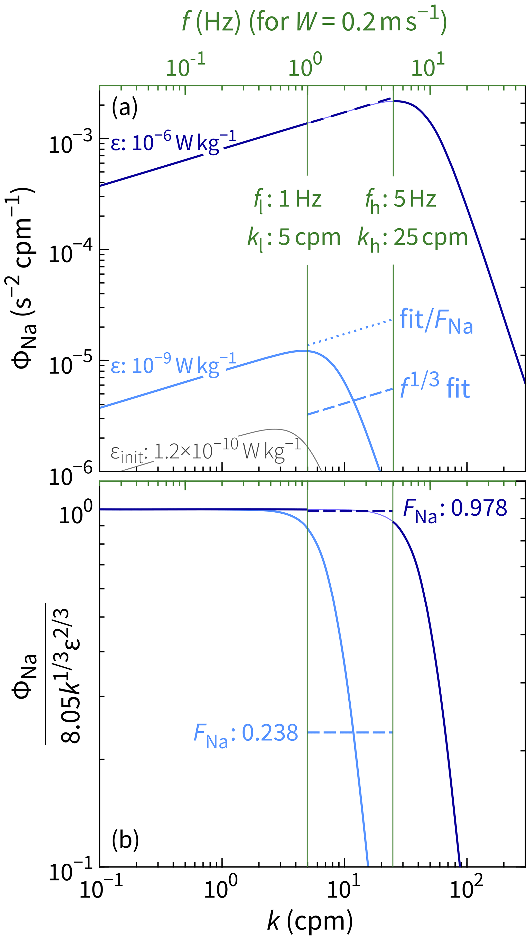
Figure 1Calculation of the correction function FNa for two values of ϵ. For W kg−1, a power law is a good approximation of the Nasmyth spectrum over the frequency range fl–fh (1–5 Hz) for a profiling speed of W=0.2 m s−1. Although the same is not true for W kg−1, we can account for the roll off with a factor of FNa. FNa can be defined in terms of either ϵ (Eq. 18) or ϵinit (Eq. 19). Panel (b) takes the former approach. In practice, we must take the latter approach, since we do not know ϵ until after it is derived from ϵinit and FNa.
Nasmyth spectra can be flattened to unity over the inertial subrange with the normalization (Fig. 1b). Values of FNa are based on the mean of these flattened spectra over the wavenumber range kl–kh (–):
To remove the dependence of the true value of ϵ, we substitute Eq. (17) to produce an implicit function for FNa, which can be solved numerically:
Note how the two forms of FNa (Eqs. 18 and 19) are defined with different arguments. For our example, FNa ( W kg−1) = W kg−1) = 0.238. Hereafter, we use the latter: FNa(ϵinit).
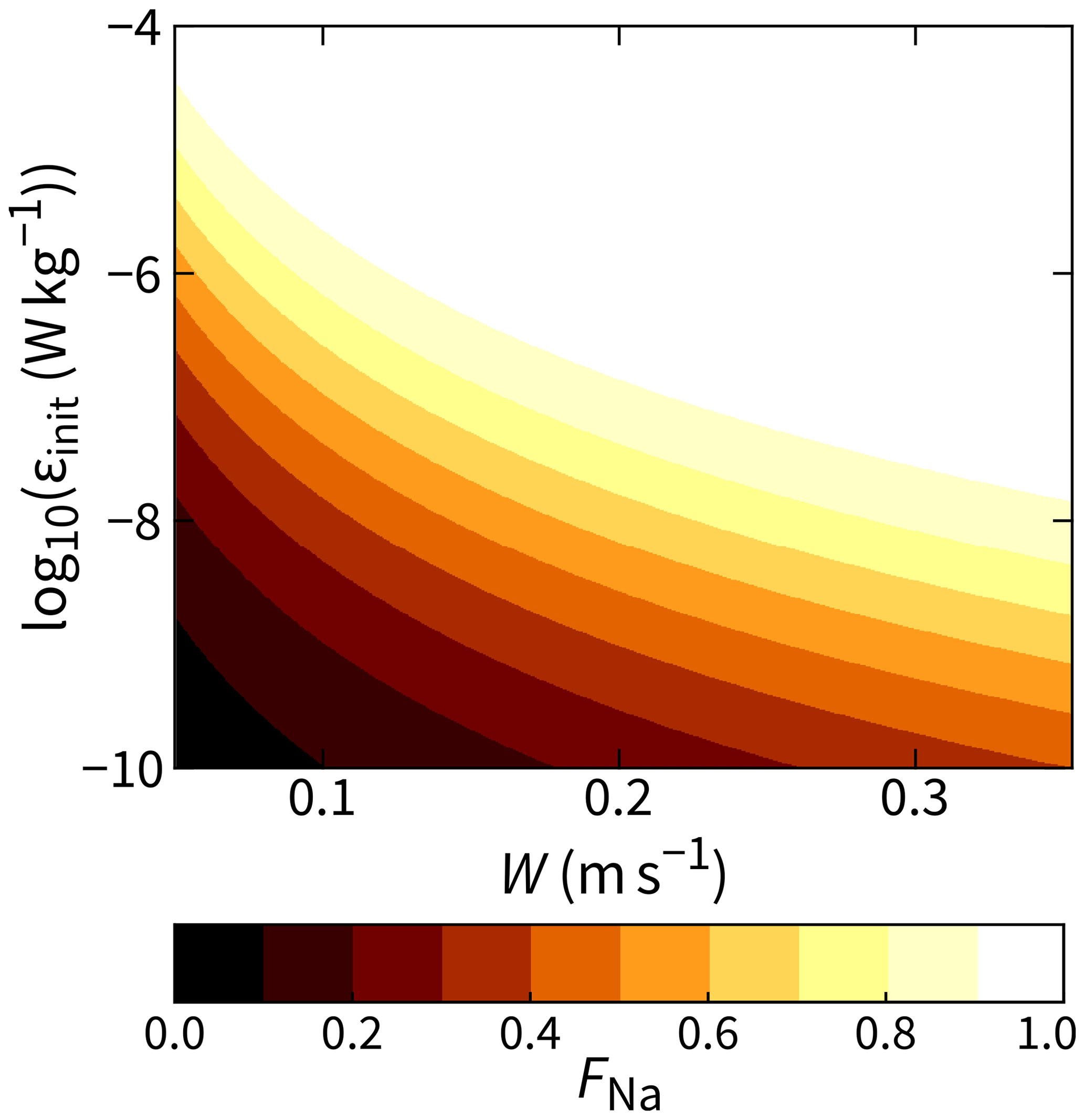
With fl and fh fixed, FNa is a function of three variables: ϵinit, W, and ν. FNa is closer to 1 (less of a correction) for larger values of ϵinit (Fig. 1). It is also closer to 1 for higher values of W (Fig. 2), since kl and kh decrease with increasing W (i.e., kl–kh move closer to the inertial subrange).
To simplify calculations in the upcoming section, we make one final change to Eq. (19) using the following substitution:
Therefore,
Think of this substitution in Eq. (20) as inverting the conventional way that is invoked. Usually, a measured shear spectrum is amplified at high wavenumbers by and is then fit to the model spectrum ΦNa. Here, instead of amplifying the measured spectrum, we reduce the model spectrum. With this latter approach, is calculated and applied only during the post-processing stage. (It changes FNa by only ∼ 5 %, since we fit over relatively low wavenumbers.)
4.2 Obtaining ϵinit from shear voltage spectra
Since ϵ can be reconstructed from ϵinit, we require an expression linking ϵinit to the shear voltage spectrum Ψs. Equating Eqs. (3) and (16) gives
where we have left out , since it has been incorporated into FNa. Rearranging and substituting gives
Then, to solve for ϵinit, we use a least-squares fit (see Appendix C):
where the sums are understood to be over the range fl–fh. The quantities α, W, and ϵinit are calculated in post-processing.
4.3 Quality control of the shear spectral fits
Measured shear spectra are often quality controlled either by manual visual inspection or, more objectively, by quantifying the level of mismatch between them and their associated model. Possible mismatch quantities include the mean absolute deviation or the variance of the ratio (e.g., Ruddick et al., 2000; Bluteau et al., 2016). We cannot calculate such quantities with our reduced scheme because we do not know what each spectrum should look like until we calculate its ϵ value in the post-processing stage. (Recall that ΦNa is a function of ϵ.) By this stage, we have lost information about the spectral shape through the summing operation in Eq. (24).
To retain at least some information about the shape of each voltage spectrum, we will split the 1–5 Hz range and compute two fits rather than one. Doing so allows for a first-order check that the spectrum over the 1–5 Hz range approximately follows the expected shape.
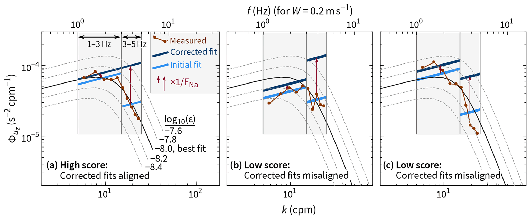
Figure 3A visual demonstration of how the ϵ fit score (Eq. 26) characterizes better and worse fits. For all three of these hypothetical spectra, ϵ values from the two fits (1–3 and 3–5 Hz) average to W kg−1. Only in panel (a), however, does the measured spectrum agree well with the Nasmyth spectrum for this ϵ value. In practice, the initial fits would be undertaken on voltage spectra; here, we are using physical units for simplicity. In all three examples, the kinematic viscosity is m2 s−1.
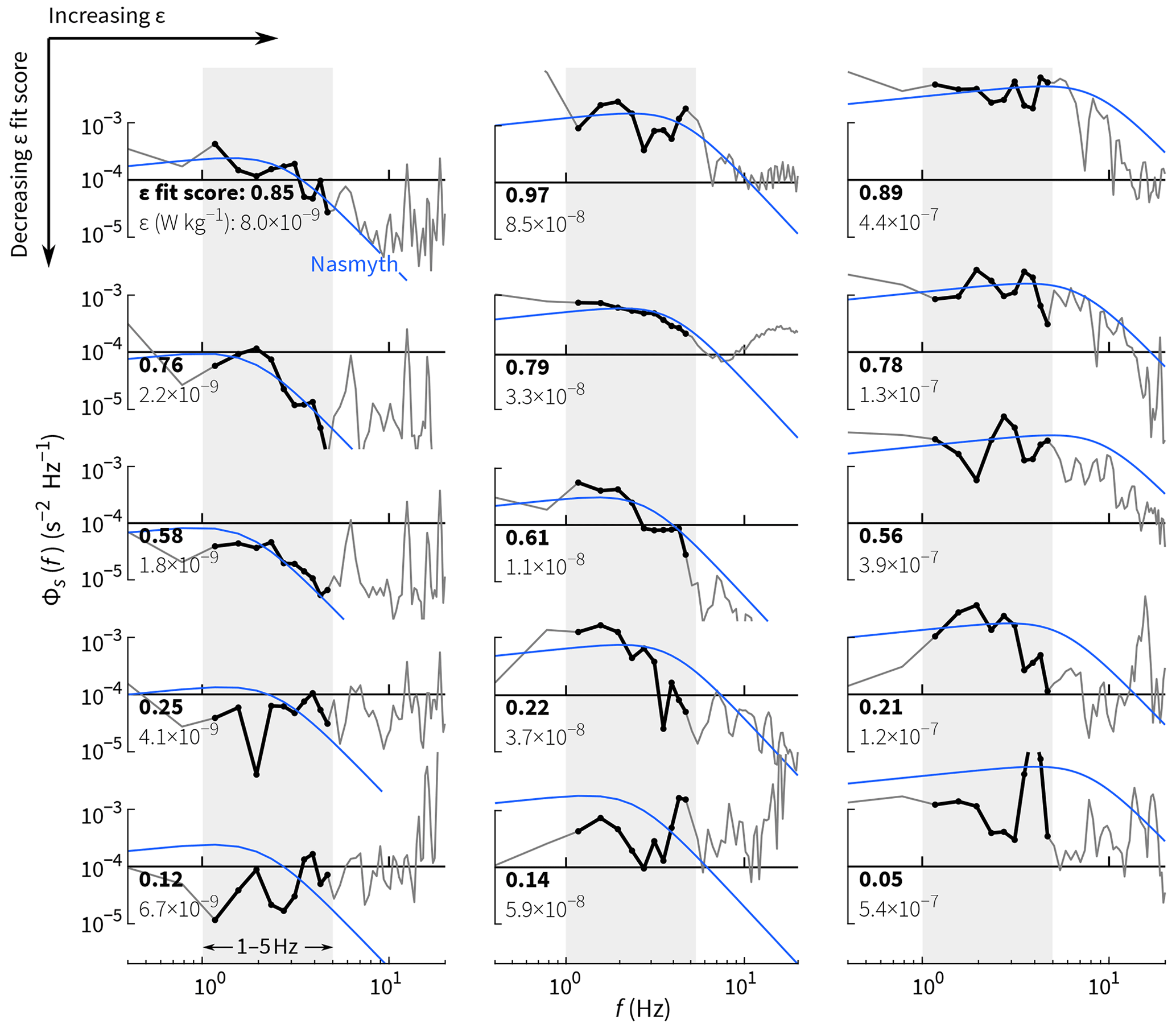
Figure 4Examples of measured shear spectra exhibiting a range of ϵ fit scores (Eq. 26). The best fits are at the top with progressively worse fits (lower scores) moving downward. The examples in each column have (left) –10−8, (middle) –10−7, and (right) –10−6 W kg−1. Each score is only based on spectral coefficients from 1–5 Hz, but lower and higher frequencies are shown for reference.
Mathematically, there is nothing special about our choice fl–fh=1–5 Hz. In theory, we can split the 1–5 Hz range into two (1–3 and 3–5 Hz) and obtain a value of ϵinit for each. These values will differ, but so will the associated values of FNa. For a measured spectrum that conforms to a Nasmyth spectrum, the two values of ϵ calculated with Eq. (17) will not differ (Fig. 3). We therefore calculate on board the sums in Eq. 24 over both fl–fm and fm–fh, where the middle frequency fm=3 Hz. (In our code, fm is actually 7.5×0.39 Hz = 2.93 Hz for the reason given in Sect. 4.1.) Hence, for each spectrum, we are able to post-process to recover two independent estimates of ϵ, denoted ϵl–m and ϵm–h. The mean of these two provides a single, final value for ϵ, and their ratio quantifies the match of a measured spectrum to a Nasmyth spectrum over the range fl–fh:
The best possible fit score is 1; the lower the score, the poorer the fit. The example spectra in Fig. 4 show that a high fit score does not necessarily imply small residuals. Rather, fits with high scores are typically those with random residuals, meaning that a given measured spectral coefficient is just as likely to be above the fit as it is to be below it. Fits with low fit scores are typically those with autocorrelated residuals, meaning that the sign and/or magnitude of a residual is correlated with that of its neighbors. In practice, we expect a range of ϵ fit scores: instantaneous and unaveraged spectra differ from the Nasmyth spectrum because they are derived from a limited sampling of a statistical process and because of non-stationarity, anisotropy, and inhomogeneity of the turbulence.
When ϵ is small (≲ 10−9 W kg−1), the fit score may be consistently low if spectral coefficients in the fm–fh range are affected by noise, and consequently ϵm–h≫ϵl–m. For such cases, we choose to use only the lower-frequency fit. We would rather have a more accurate estimate of ϵ and forgo the fit score than have a biased-high ϵ value with a biased-low fit score. (Either way, the small values of ϵ in question will have minimal effect on any averages, given that turbulence distributions have high kurtosis, so high values dominate means.) Specifically,
where the threshold is equivalent to , with η being the Kolmogorov length scale estimated from ϵl–m. For reference, ΦNa peaks at and rolls off to 11 % of its maximum by (see Eq. 15).
To test the accuracy of the shear reduction scheme described in the previous section, we apply it retrospectively to the dataset from the 2019 test cruise (Sect. 2). We compare the results to those obtained with the standard processing scheme. This standard scheme (Appendix D) features a more sophisticated despiking routine than that used for our reduced scheme, which employs a 3-standard-deviations threshold filter (Appendix E).
A profile-by-profile comparison of the two schemes is shown in Fig. 5. The comparison is then extended to all 650 profiles (> 77 000 segments of shear), where we find that ϵ from the reduced scheme () is within a factor of 2 of that from the standard scheme 87 % of the time over the full range of measured values, W kg−1 (Fig. 6a–b). For comparison, in only 72 % do we obtain a factor-of-2 agreement between the two independent values of ϵ measured on the unit with two working shear probes (not shown). Further, to obtain this 87 % agreement, we clearly need the correction function FNa: Fig. 6c shows that the uncorrected values ϵinit only have 1 : 1 agreement with ϵ from the standard scheme if W kg−1. For the lowest values of ϵ, the ratio is closer to 1 : 30.
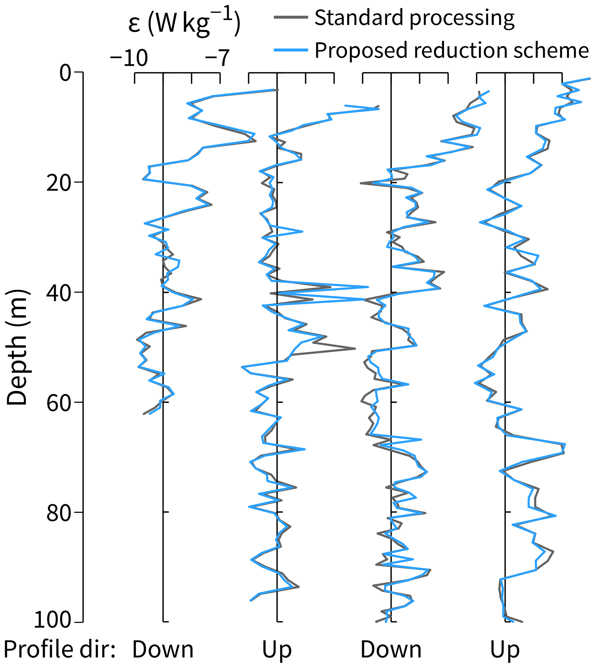
Figure 5Testing the proposed data reduction scheme for shear measurements against the standard processing approach. One upward and one downward profile from each of the two FCS units were arbitrarily chosen for this comparison.
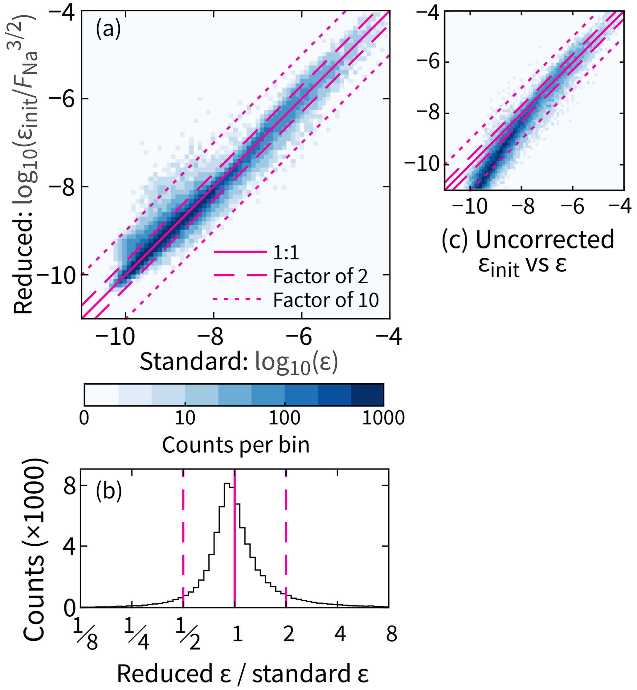
Figure 6Statistical test of the proposed data reduction scheme for ϵ based on all 650 profiles (77 000 segments). (a) A comparison that includes the dependence on ϵ. (b) Further summarized data that exclude this dependence. (c) Same as for panel (a) but uncorrected (FNa = 1).
To demonstrate the ability of the ϵ fit score to characterize spectra, we show two-dimensional histograms of non-dimensionalized spectral coefficients from all 77 000 measured shear spectra separated into three classes based on their ϵ fit score: 0.67–1.00, 0.33–0.67, and 0.00–0.33. Only the lowest-scoring class fails to collapse to the Nasmyth spectrum (Fig. 7c, f).
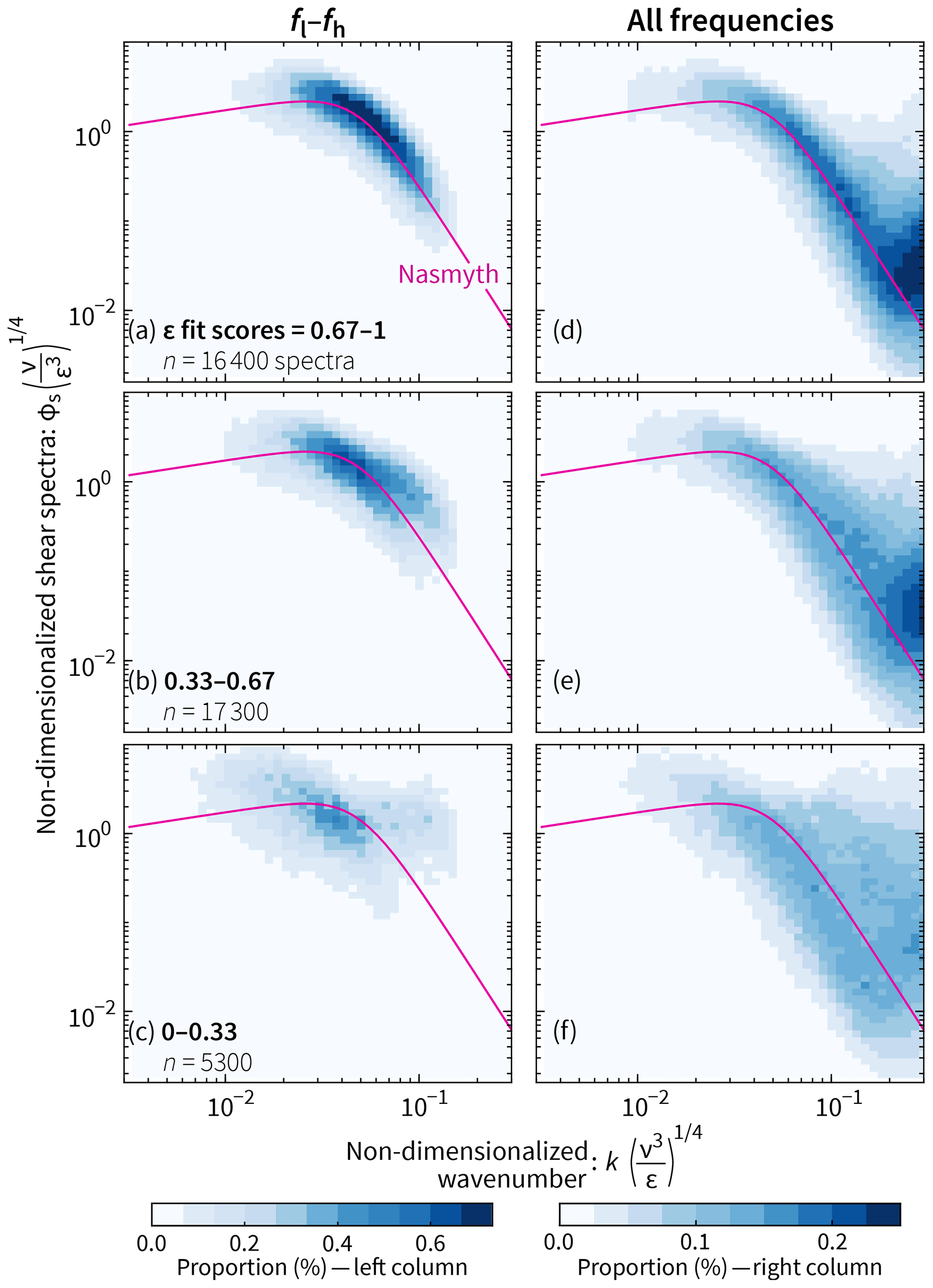
Figure 7As the ϵ fit score decreases from top to bottom, there is a corresponding decrease in the level of agreement and tightness of spread between (i) non-dimensionalized, measured shear spectra and (ii) the Nasmyth spectrum. The two-dimensional histograms in the left column include only spectral coefficients with frequencies between fl and fh; those in the right column include all frequencies. The total number of spectra in this figure is lower than in Fig. 10 because some low-ϵ spectra do not have scores (Eq. 27) and because one of the shear probes failed (Sect. 2).
The scheme to reduce fast-thermistor data to enable measurement of χ is much like the scheme to reduce shear data. As in Sect. 4, we first show how we summarize a model spectrum in terms of a power law fit and a correction factor. (In this case, the correction factor partly depends on the values of ϵ calculated in Sect. 4.) Then we derive the implementation in terms of voltages and calculate a spectral-fit metric.
6.1 Summarizing Kraichnan spectra with f1 fits
Here we take the Kraichnan spectrum ΦKr (Kraichnan, 1968) as our model; for its low-wavenumber approximation, we use the viscous–convective subrange, which scales as k+1. In units of K2 m−2 cpm−1, ΦKr and its approximation are as follows (e.g., Peterson and Fer, 2014):
where the Batchelor length scale , and q is a constant taken to be 5.26. This expression does not include a inertial–convective subrange, which we ignore here, as it increases by less than 1 % the integral of the temperature gradient spectrum from k=0 to k=∞ and therefore has negligible effect on our results.
A fit against Eq. (29) can be rearranged to give χinit, which is related to χ through the correction function FKr as
FKr is not raised to a power like FNa (Eq. 17). For small values of k, ΦKr∝χ, whereas .
The derivation of FKr is equivalent to FNa. We therefore present only the result:
Note that depends on the underestimate χinit, whereas it depends on the “true” or “corrected” value of ϵ as calculated in Sect. 4.
6.2 Obtaining χinit from fast-thermistor voltage spectra
Like we did for ϵinit in Sect. 4.2, we derive the expression for χinit in three steps. First, equate the right-hand sides of Eqs. (11) and (29) (excluding the transfer function , which is incorporated into Eq. 31):
Then, rearrange while substituting to get
Finally, solve for χinit using a least-squares fit (Appendix C):
6.3 Quality control of the temperature gradient spectral fits
The approach to quality controlling the fast-thermistor data is the same as that for shear (Sect. 4.3). That is, we fit ΨTt over fl–fm and fm–fh (1–3 and 3–5 Hz). This ultimately provides two estimates of χ for each spectrum, which are combined as follows:
We do not apply a low χ threshold equivalent to Eq. (27).
Profiles of χ from the reduced scheme compare well to the standard processing, albeit with a small bias in one direction for low values and in the other direction for high values (Fig. 8). Across all values, the two approaches agree within a factor of 2 78 % of the time (Fig. 9). By comparison, 82 % of segments exhibit a factor-of-2 agreement between χ values from the two fast thermistors on the same unit.
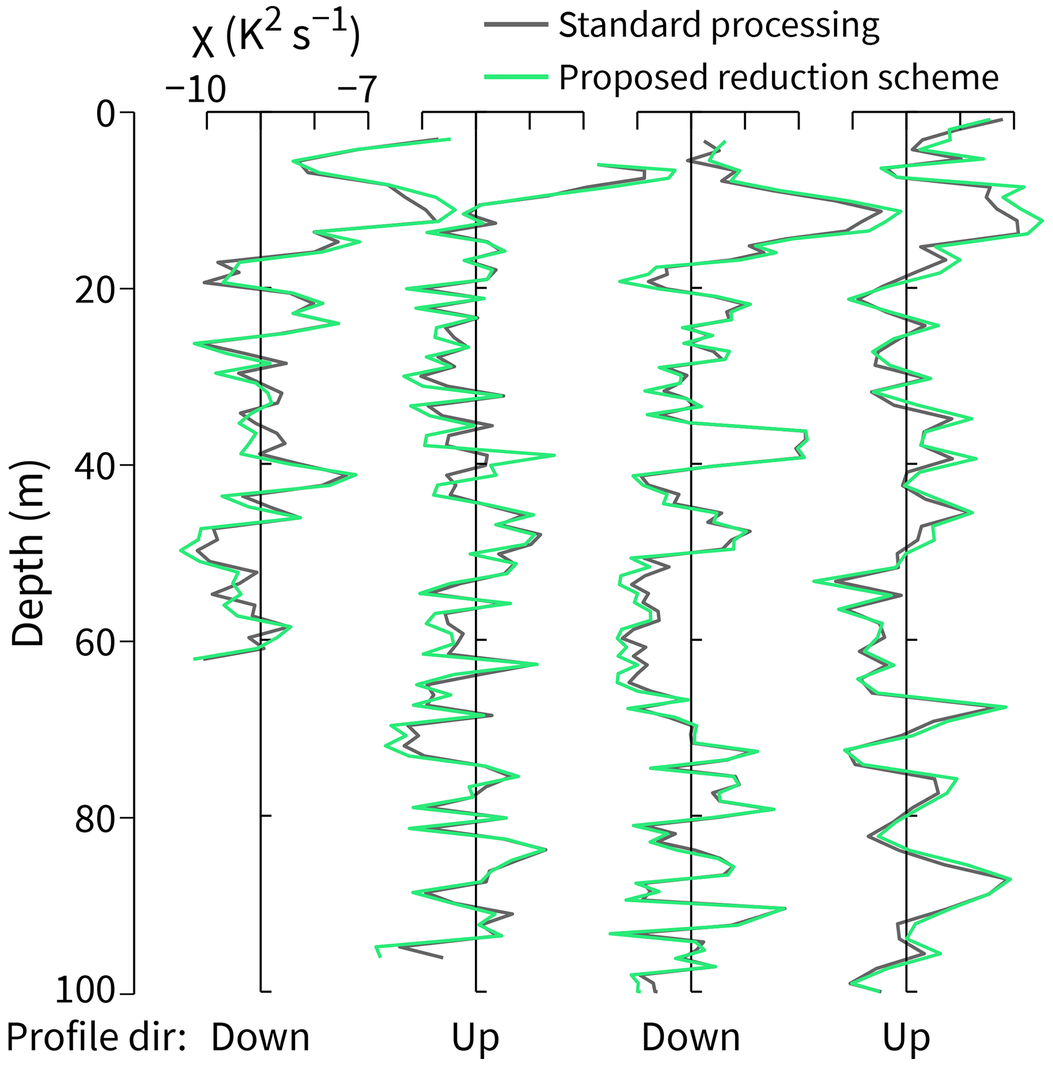
Figure 8Testing the proposed data reduction scheme for fast-thermistor measurements. The profiles used are the same as those chosen in Fig. 5.
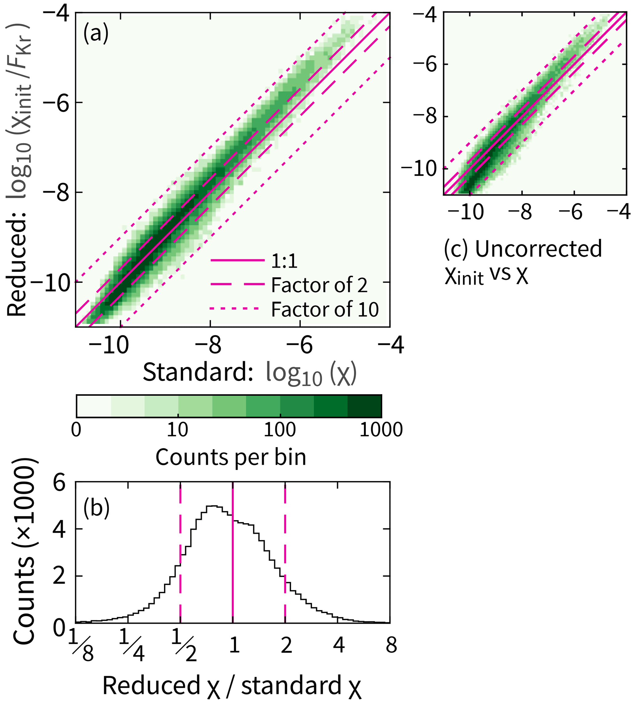
Figure 9Statistical test of the proposed data reduction scheme for χ. Equivalent to Fig. 6, except for the use of χ instead of ϵ. In total, there are 100 000 segments of data.
Compared to shear spectra, non-dimensionalized temperature gradient spectra have lower fit scores. Especially for the lowest fit scores, the measured temperature gradient spectra tend to be too high at lower frequencies and too low at frequencies near fh (Fig. 10a–c). As frequency increases beyond fh, the effects of noise and thermal-response corrections (Appendix A) begin to dominate.
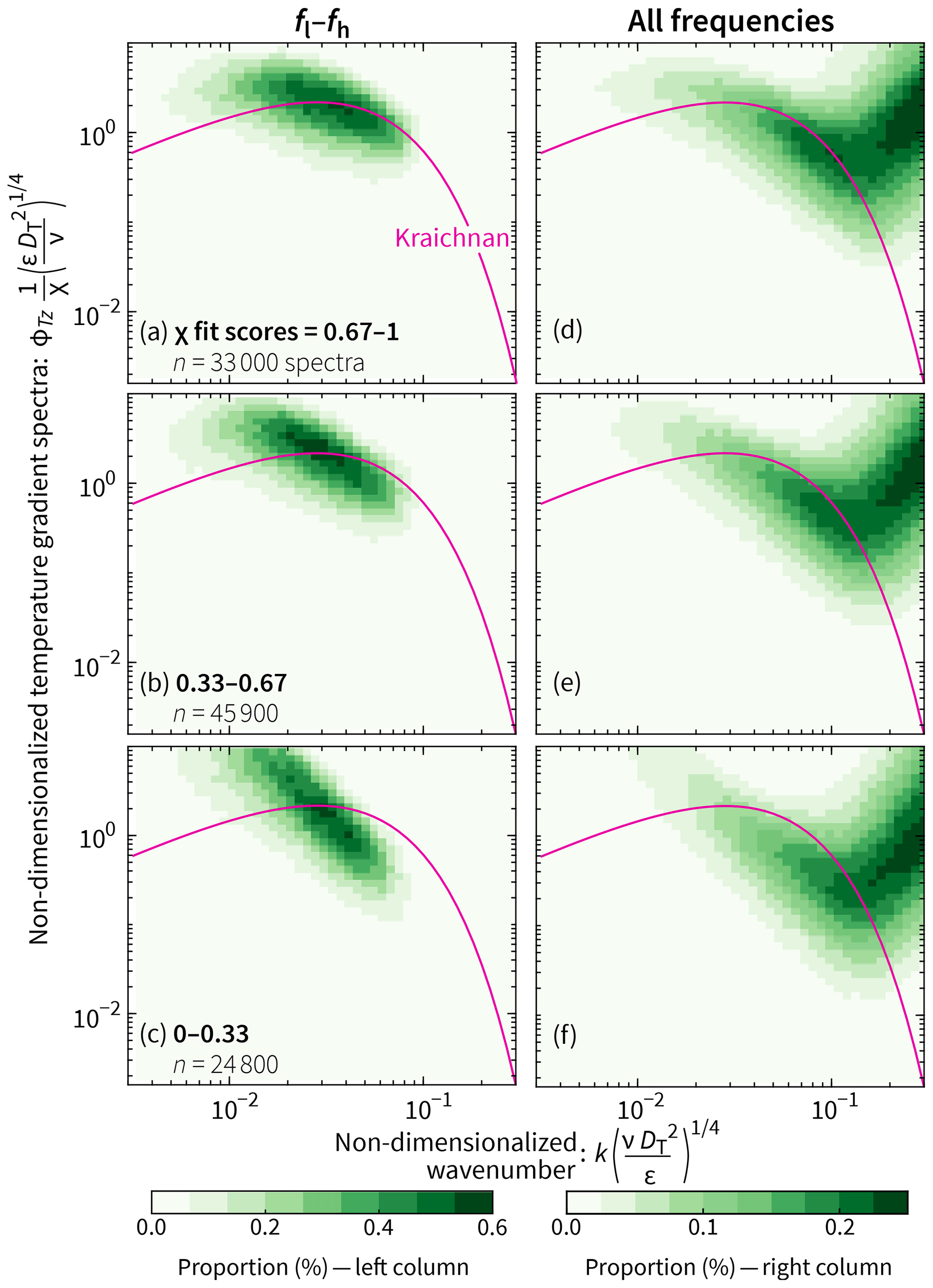
There are three reasons for the poorer fits to temperature gradient spectra compared to that for shear. First, shapes of temperature gradient spectra are often more variable; the best choice for the non-dimensional spectral model can be debated (e.g., Sanchez et al., 2011). Second, the temperature gradient fits depend on ϵ, so uncertainties in ϵ propagate into the calculation of χ. Third, for our 2019 experiment, the recorded temperature gradient signals were occasionally affected by digitization noise as a consequence of sampling mixed layers. (Shear signals were not affected by digitization noise.)
8.1 Setting the scheme's parameters
Our scheme requires a few user-defined parameters: fl, fh, Nseg, and Nfft. For this paper, we based these partly on the profiling speed and scientific goals of FCS. For a different profiler, we suggest the following:
-
Choose fh based on a typical profiling speed such that cpm for a nominal profiling speed W. For a wide range of ϵ values, 25 cpm is close to, or beyond, the peak of the Nasmyth spectrum (Fig. 1). As an example, if FCS profiled at ∼ 0.5 m s−1, we would consider setting fh≈12 Hz.
-
Ensure that there are no known issues such as vibrations that are likely to adversely affect spectral coefficients within the fl–fh range. If, however, there are known issues within the desired frequency range, then an alternative approach (one that we did not test) is to use accelerometer signals to correct spectra that are contaminated by vibrations (Levine and Lueck, 1999; Goodman et al., 2006).
-
Define fl and fh separately for shear and temperature gradient if appropriate. Although we set them to be equal here, this is not necessary.
-
Use more than two fitting bands if desired. We use only two bands (1–3 and 3–5 Hz) so as to minimize the file size to be transmitted, but there is nothing preventing there being three or more bands (e.g., adding a 5–7 Hz band). Indeed, this would enable improved estimates of the fit scores (Eqs. 26 and 36) and more flexibility to discard noise-affected bands as in Eq. (27). If file size is less of an issue such that it is possible to send back fit values for many more than two bands, then the Rainville et al. (2017) scheme outlined in Sect. 1 may be a better choice than ours.
-
Choose Nseg and Nfft based on scientific goals and, possibly, any logistical constraints; the data reduction scheme is agnostic to these numbers. For example, at the expense of vertical resolution, we could halve the file size of our transmitted dataset by doubling Nseg from 512 to 1024.
-
Reasonable choices for Nfft are or , which correspond to three or seven half-overlapping subsegments, respectively. There is little to be gained by dividing a segment into even more subsegments so as to produce smoother spectra before fitting. As Ruddick et al. (2000) note, the choice is analogous to fitting a line to 20 points at once or first clumping them into groups of, say, five and then fitting the four averaged points.
8.2 Evaluating the reduced data
One step that cannot be automated is the heuristic evaluation of the reduced turbulence data after they have been converted from voltage quantities to physical ones. For this evaluation, we recommend looking into multiple quantities. First consider the fit scores (Eqs. 26 and 36). We recommend discarding any ϵ or χ values with an associated fit score lower than 0.33. Note, however, that these scores are not a perfect measure of fit. They should be used together with other quality control checks such as comparing
-
W and Wmin (Eqs. 13 and 14) to check whether the profiling speed is constant over a segment;
-
ϵ values from the two shear probes; and
-
turbulent features in successive profiles.
The last point is most applicable for a vertical profiler cycling rapidly – for example, twice per hour for FCS. In this case, the profiler is nominally sampling the same vertical fragment of the ocean on a timescale comparable to that over which turbulence evolves. In our experience, many turbulent patches extend over 5–10 profiles.
Recall, also, that all uncertainty in ϵ propagates into the calculation of χ (Sect. 7). If ϵ for a given segment cannot be trusted, neither can χ.
We have developed a data reduction scheme applicable to vertical profiling of turbulence variables in which each ∼ 5 s segment is distilled to 12 quantities (Scheme 1). In post-processing, we reconstruct estimates of ϵ and χ, associated quality control metrics, and other quantities such as the temperature and profiling speed. The raw data that go into the 12 quantities are seven different voltages (VP; VT and VTt for each thermistor; and Vs for each shear probe). Hence, for each 512-element segment, we effectively reduce the data by a factor of .

Scheme 1Summary of the data reduction scheme. Each 512-element segment of data is ultimately compressed down to the 12 highlighted quantities that are then transmitted. These are calibrated and/or converted into turbulence quantities in post-processing.
This reduction compresses the output data file size for each dive from megabytes to kilobytes. For example, the total amount of data per dive (two profiles) can be estimated assuming our nominal dive depth and profiling velocity of 120 m and 0.2 m s−1. Each dive creates m (0.2 m s quantities. Transmitting each quantity as a 16-bit float or integer equates to approximately 6 kB per dive. This can be reduced by one-third if the spectral-fit metrics are suitably scaled logarithmically and then transmitted as 8-bit integers.
One luxury we lose is the ability to inspect the raw signals. Typically this would help to (i) cultivate faith in the data, (ii) flag which segments to discard, and (iii) inform work-arounds such as filtering out potential narrowband vibrations in shear spectra. Our scheme accounts for this constraint in two ways. First, we fit spectra over relatively low frequencies (1–5 Hz) that are unlikely to be affected by noise or vibration. Second, we reduce the data in a way that uses as little arithmetic as possible. Obviously, we cannot reverse-engineer the raw signals, but by making the onboard calculations simple, we give ourselves the best chance to later fix or identify any unforeseen issues.
Although the onboard reduction eliminates possibilities in how we process turbulence data, it opens up possibilities in how we obtain turbulence data. By visualizing how turbulence evolves over successive dives in near-real time, we can concentrate on regions of interest by adapting the dive schedule to profile more frequently or to different depths. If instead we encounter quiescent periods, we might consider profiling less frequently, thereby conserving battery life. Our ultimate objective is to treat FCS floats as expendable.
Voltage signals from shear probes and thermistors are a smoothed representation of the true environmental signal. If the smoothing is a spatial effect, it is described by a transfer function H2(k). If the smoothing is a temporal effect, it is more natural to use H2(f). We can use these interchangeably because f=Wk, and therefore H2(f)=H2(Wk). For FCS, there are three components to the transfer function for each sensor:
where we have used the following shorthand: SP is shear probe, FT is fast thermistor, AA is anti-aliasing, and D is digital. We describe each of these in turn.
Shear probes built and calibrated by the Ocean Mixing Group are very close in dimension to those examined by Ninnis (1984), who measured their wavenumber response and represented it as
where a0=1.000, , , a3=5.503, , and k0=170 cpm.
Temporal averaging of temperature at high frequencies due to the thermal response of the fast thermistor is modeled using a double-pole filter:
where the cut-off frequency fc=30 Hz. This comes from Nash et al. (1999), who measured the frequency response for two different thermistors on an instrument profiling at 0.3 m s−1 and found cut-off frequencies of 25.1 and 36.7 Hz (see their Fig. A2). The 30 Hz value is the approximate mean of these two values.
Raw shear and thermistor voltage signals are both subject to two filters. First, an analog anti-aliasing filter (two-pole Butterworth) with an fc=40 Hz cut-off:
After the analog signal is anti-aliased, it is digitized at 400 Hz. Before subsampling to the final 100 Hz output, the signal is digitally filtered. For the 2019 FCS cruise, the signal was convolved with a symmetric 29-element kernel in which the first 15 elements were
This is a sinc kernel but with negative values set to zero. (We are currently investigating better choices for future implementations). The filter has a half-power (−3 db) point at 25 Hz.
Early in our processing routine, we partition the raw voltage signals into 512-element segments. In order to discard the segments in which FCS was not profiling, we need robust (yet simple) criteria that demarcate the start and end of a profile. For the start, we search for the first three consecutive segments in which Wmin>0.05 m s−1. For the end, we swap the inequality.
A drawback of this approach is the appearance of a quantity in physical units (0.05 m s−1). This is the one instance where we hard code a calibration coefficient in the onboard software rather than applying it in post-processing. Fortunately, the relevant coefficient can be approximated as constant: C2P = 76.7 psi V−1 (barring a redesign of the circuitry or the use of a different brand or model of pressure sensor). For the two units already built, C2P=76.81 psi V−1 and 76.53 psi V−1. By comparison, among the four shear probes on the two units, the calibration coefficients vary by 30 %.
At least for the initial implementation of our scheme, we do not include an algorithm to detect the surface to within centimeters. Doing so would let us work backward to put our uppermost depth bin as close to the surface as possible. However, we expect that this could be a fragile part of the scheme. Further, FCS lacks a micro-conductivity sensor, which is likely the sensor best suited for identifying the air–sea interface (e.g., Ward et al., 2014).
Without surface detection, the depths of the uppermost bins will be realized randomly. In the worst cases, we would discard the top ∼ 1 m (5 s at ∼ 0.2 m s−1). To alleviate this, we may use half-overlapping bins near the surface. The exact implementation will be determined later in the development.
In this paper, we use power law fits to derive turbulence quantities: and ΨTt=Aχf1, where Aϵ and Aχ are substitutes for the expressions in Eqs. (23) and (33). With only a single parameter for each fit, implementing a least-squares fit is easy.
Assume we are fitting the vector Ψi to the function where n is either or 1. The sum of squared residuals is therefore
The minimum with respect to A is where the derivative is zero:
Hence,
We had originally intended to find A by following Becherer and Moum (2017), who were fitting spectra. Their simpler method, , is equivalent to a least-squares fit, except the quantity minimized is the sum of the squares of the adjusted residuals, where adjusted means divided by fn. Differences can be ignored when but not when n=1.
The standard processing of FCS turbulence data differs from the reduced scheme in three ways. First, raw data are despiked differently (Appendix E). Second, the 100 Hz raw voltage signals are calibrated into physical quantities right away. Hence, means and spectra are calculated in physical units and not in voltage units. Third, the integration of spectra occurs over a variable wavenumber band, which is found iteratively.
When integrating shear spectra (after correction; see Appendix A) to find ϵ, we follow the approach used for the Chameleon profiler (Moum et al., 1995). A first estimate of ϵ is made by integrating over k=4–10 cpm. This value provides a first estimate of the Kolmogorov wavenumber . (The lower limit for Chameleon is 2 cpm, but we increase this for FCS given its slower profiling speed and hence the possibility of contamination by waves at lower wavenumbers.) The upper integral limit is then set to 0.5ks (with a minimum of 10 cpm and a maximum of 45 cpm). The Nasmyth spectra (Eq. 15) is integrated over the same wavenumber range. If the measured and Nasmyth integrals are within 1 %, then ϵ is set to be equal to the integral of the Nasmyth spectrum over all k. Otherwise, ϵ and ks are adjusted iteratively until the two integrals agree.
A similar but non-iterative approach is used for integrating Tz spectra to find χ. The model spectrum is the Kraichnan spectrum (Eq. 28), and again, the lower limit of integration is 4 cpm. The upper limit is the Batchelor wavenumber (with a maximum defined by kW=15 Hz).
To properly despike the raw output of a shear probe requires several steps. Lueck et al. (2018) describe a process in which the signal is high-passed, then rectified, and then low-passed to derive a measure of the local variance. A value is defined as a spike if it is more than 8 times (or a similar threshold) higher than the local variance. Spikes are replaced with an average based on surrounding points. This process is then repeated on the new signal and so on until no spikes are identified.
In our standard processing of FCS data, we use the Lueck et al. (2018) despiking routine. For our data reduction scheme, we use an approach that is easier to implement and quicker to compute, albeit one that is less precise. For each 512-element segment of data, a spike is defined as any data point larger than 3 standard deviations from the mean. These spikes are replaced by the mean of the remaining values in the segment.
Our MATLAB implementation of the processing code is available from https://doi.org/10.5281/zenodo.7644701 (Hughes and Vutukur, 2023) or https://github.com/OceanMixingGroup/flippin-chi-solo (last access: 17 February 2023).
Raw and processed data for the 2019 experiment are available at https://doi.org/10.5281/zenodo.5719505 (Hughes, 2022) or https://kghughes.com/data (last access: 17 February 2023).
KGH designed the reduction scheme and led the writing of the paper. All authors contributed to the final version. JNM and DLR lead the development of the FCS profiler on which much of the paper is based.
The contact author has declared that none of the authors has any competing interests.
Publisher’s note: Copernicus Publications remains neutral with regard to jurisdictional claims in published maps and institutional affiliations.
This work was funded by the Office of Naval Research under grant nos. N00014-17-1-2700 (OSU) and N00014-17-1-2762 (SIO) and continued as part of the ARCTERX (Island Arc Turbulent Eddy Regional Exchange) program under grant nos. N00014-21-1-2878 (OSU), N00014-21-1-2762, and N00014-21-1-2747 (SIO). Engineers who contributed to the design and construction of FCS and its sensors are Craig Van Appledorn, Kerry Latham, Pavan Vutukur, and Mark Borgerson (all from OSU) and Ben Reineman, Kyle Grindley, and Jeff Sherman from SIO. Aurélie Moulin executed initial turbulence processing, and Emily Shroyer provided many helpful comments on early drafts. Thanks to the reviewers, including Cynthia Bluteau and Toshiyuki Hibiya.
This research has been supported by the Office of Naval Research (grant nos. N00014-17-1-2700, N00014-17-1-2762, N00014-21-1-2878, N00014-21-1-2762, N00014-21-1-2747).
This paper was edited by Katsuro Katsumata and reviewed by Toshiyuki Hibiya and Cynthia Bluteau Toshiyuki Hibiya and one anonymous referee.
Becherer, J. and Moum, J. N.: An efficient scheme for onboard reduction of moored χpod data, J. Atmos. Ocean. Tech., 34, 2533–2546, https://doi.org/10.1175/JTECH-D-17-0118.1, 2017. a, b
Bluteau, C. E., Jones, N. L., and Ivey, G. N.: Estimating turbulent dissipation from microstructure shear measurements using maximum likelihood spectral fitting over the inertial and viscous subranges, J. Atmos. Ocean. Tech., 33, 713–722, https://doi.org/10.1175/JTECH-D-15-0218.1, 2016. a, b
Goodman, L., Levine, E. R., and Lueck, R. G.: On measuring the terms of the turbulent kinetic energy budget from an AUV, J. Atmos. Ocean. Tech., 23, 977–990, https://doi.org/10.1175/JTECH1889.1, 2006. a
Greenan, B. J. W., Oakey, N. S., and Dobson, F. W.: Estimates of dissipation in the ocean mixed layer using a quasi-horizontal microstructure profiler, J. Phys. Oceanogr., 31, 992–1004, https://doi.org/10.1175/1520-0485(2001)031<0992:EODITO>2.0.CO;2, 2001. a
Hughes, K.: A turbulence data reduction scheme for autonomous and expendable profiling floats: datasets, Zenodo [data set], https://doi.org/10.5281/zenodo.5719505, 2022. a
Hughes, K. and Vutukur, P.: OceanMixingGroup/flippin-chi-solo: Version 1, Version v1, Zenodo [code], https://doi.org/10.5281/zenodo.7644701, 2023. a
Kraichnan, R. H.: Small-scale structure of a scalar field convected by turbulence, Phys. Fluids, 11, 945–953, https://doi.org/10.1063/1.1692063, 1968. a
Levine, E. R. and Lueck, R. G.: Turbulence measurement from an autonomous underwater vehicle, J. Atmos. Ocean. Tech., 16, 1533–1544, https://doi.org/10.1175/1520-0426(1999)016<1533:TMFAAU>2.0.CO;2, 1999. a, b
Lueck, R.: Calculating the rate of dissipation of turbulent kinetic energy, Tech. rep., Rockland Scientific, https://rocklandscientific.com/support/knowledge-base/technical-notes/ (last access: 2 August 2018), 2013. a
Lueck, R., Murowinski, E., and McMillan, J.: A guide to data processing: ODAS Matlab library v4.3., Tech. rep., Rockland Scientific, https://rocklandscientific.com/support/knowledge-base/technical-notes/ (last access: 6 August 2021), 2018. a, b
Lueck, R. G., Wolk, F., and Yamazaki, H.: Oceanic velocity microstructure measurements in the 20th century, J. Oceanogr., 58, 153–174, https://doi.org/10.1023/A:1015837020019, 2002. a
Merckelbach, L. M. and Carpenter, J. R.: Ocean glider flight in the presence of surface waves, J. Atmos. Ocean. Tech., 38, 1265–1275, https://doi.org/10.1175/JTECH-D-20-0206.1, 2021. a
Moum, J. N. and Nash, J. D.: Mixing measurements on an equatorial ocean mooring, J. Atmos. Ocean. Tech., 26, 317–336, https://doi.org/10.1175/2008JTECHO617.1, 2009. a
Moum, J. N., Gregg, M. C., Lien, R. C., and Carr, M. E.: Comparison of turbulence kinetic energy dissipation rate estimates from two ocean microstructure profilers, J. Atmos. Ocean. Tech., 12, 346–366, https://doi.org/10.1175/1520-0426(1995)012<0346:COTKED>2.0.CO;2, 1995. a, b
Moum, J. N., Rudnick, D. L., Shroyer, E. L., Hughes, K. G., Reineman, B. D., Grindley, K., Sherman, J., Vutukur, P., Van Appledorn, C., Latham, K., Moulin, A. J., and Johnston, T. M. S.: Flippin' χSOLO, an upper ocean autonomous turbulence profiling float, J. Atmos. Ocean. Tech., in review, 2023. a
Nash, J. D., Caldwell, D. R., Zelman, M. J., and Moum, J. N.: A thermocouple probe for high-speed temperature measurement in the ocean, J. Atmos. Ocean. Tech., 16, 1474–1482, https://doi.org/10.1175/1520-0426(1999)016<1474:ATPFHS>2.0.CO;2, 1999. a
Nasmyth, P. W.: Oceanic turbulence, PhD thesis, Univ. British Columbia, https://doi.org/10.14288/1.0302459, 1970. a
Ninnis, R.: The effects of spatial averaging on airfoil probe measurements of oceanic velocity microstructure, PhD thesis, University of British Columbia, https://doi.org/10.14288/1.0053131, 1984. a
Oakey, N. S.: Determination of the rate of dissipation of turbulent energy from simultaneous temperature and velocity shear microstructure measurements, J. Phys. Oceanogr., 12, 256–271, https://doi.org/10.1175/1520-0485(1982)012<0256:DOTROD>2.0.CO;2, 1982. a
Osborn, T. R.: Vertical profiling of velocity microstructure, J. Phys. Oceanogr., 4, 109–115, https://doi.org/10.1175/1520-0485(1974)004<0109:VPOVM>2.0.CO;2, 1974. a
Peterson, A. K. and Fer, I.: Dissipation measurements using temperature microstructure from an underwater glider, Methods Oceanogr., 10, 44–69, https://doi.org/10.1016/j.mio.2014.05.002, 2014. a
Rainville, L., Gobat, J. I., Lee, C., and Shilling, G.: Multi-month dissipation estimates using microstructure from autonomous underwater gliders, Oceanography, 30, 49–50, https://doi.org/10.5670/oceanog.2017.219, 2017. a, b, c
Roemmich, D., Riser, S., Davis, R., and Desaubies, Y.: Autonomous profiling floats: Workhorse for broad-scale ocean observations, Mar. Technol. Soc. J., 38, 21–29, https://doi.org/10.4031/002533204787522802, 2004. a
Roemmich, D., Alford, M. H., Claustre, H., Johnson, K., King, B., Moum, J., Oke, P., Owens, W. B., Pouliquen, S., Purkey, S., Scanderbeg, M., Suga, T., Wijffels, S., Zilberman, N., Bakker, D., Baringer, M., Belbeoch, M., Bittig, H. C., Boss, E., Calil, P., Carse, F., Carval, T., Chai, F., Conchubhair, D., d'Ortenzio, F., Dall'Olmo, G., Desbruyeres, D., Fennel, K., Fer, I., Ferrari, R., Forget, G., Freeland, H., Fujiki, T., Gehlen, M., Greenan, B., Hallberg, R., Hibiya, T., Hosoda, S., Jayne, S., Jochum, M., Johnson, G. C., Kang, K., Kolodziejczyk, N., Körtzinger, A., Traon, P.-Y. L., Lenn, Y.-D., Maze, G., Mork, K. A., Morris, T., Nagai, T., Nash, J., Garabato, A. N., Olsen, A., Pattabhi, R. R., Prakash, S., Riser, S., Schmechtig, C., Schmid, C., Shroyer, E., Sterl, A., Sutton, P., Talley, L., Tanhua, T., Thierry, V., Thomalla, S., Toole, J., Troisi, A., Trull, T. W., Turton, J., Velez-Belchi, P. J., Walczowski, W., Wang, H., Wanninkhof, R., Waterhouse, A. F., Waterman, S., Watson, A., Wilson, C., Wong, A. P. S., Xu, J., and Yasuda, I.: On the future of Argo: A global, full-depth, multi-disciplinary array, Front. Mar. Sci., 6, 439, https://doi.org/10.3389/fmars.2019.00439, 2019a. a
Roemmich, D., Sherman, J. T., Davis, R. E., Grindley, K., McClune, M., Parker, C. J., Black, D. N., Zilberman, N., Purkey, S. G., Sutton, P. J. H., and Gilson, J.: Deep SOLO: A Full-Depth Profiling Float for the Argo Program, J Atmos. Ocean. Tech., 36, 1967–1981, https://doi.org/10.1175/JTECH-D-19-0066.1, 2019b. a
Ruddick, B., Anis, A., and Thompson, K.: Maximum likelihood spectral fitting: The Batchelor Spectrum, J. Atmos. Ocean. Tech., 17, 1541–1555, https://doi.org/10.1175/1520-0426(2000)017<1541:MLSFTB>2.0.CO;2, 2000. a, b
Sanchez, X., Roget, E., Planella, J., and Forcat, F.: Small-scale spectrum of a scalar field in water: The Batchelor and Kraichnan models, J. Phys. Oceanogr., 41, 2155–2167, https://doi.org/10.1175/JPO-D-11-025.1, 2011. a
Shroyer, E. L., Rudnick, D. L., Farrar, J. T., Lim, B., Venayagamoorthy, S. K., St. Laurent, L. C., Garanaik, A., and Moum, J. N.: Modification of upper-ocean temperature structure by subsurface mixing in the presence of strong salinity stratification, Oceanography, 29, 62–71, https://doi.org/10.5670/oceanog.2016.39, 2016. a
Ward, B., Fristedt, T., Callaghan, A. H., Sutherland, G., Sanchez, X., Vialard, J., and ten Doeschate, A.: The Air–Sea Interaction Profiler (ASIP): An autonomous upwardly rising profiler for microstructure measurements in the upper ocean, J. Atmos. Ocean. Tech., 31, 2246–2267, https://doi.org/10.1175/JTECH-D-14-00010.1, 2014. a
- Abstract
- Introduction
- The Flippin' χSOLO (FCS)
- Conversion of measured voltages to physical units
- Reduction of shear data
- Test of the reduction scheme for ϵ
- Reduction of fast-thermistor data
- Test of the reduction scheme for χ
- Recommendations
- Conclusions
- Appendix A: Transfer functions for FCS sensors
- Appendix B: Identifying the start and end of a profile
- Appendix C: Least-squares fitting of power laws
- Appendix D: Standard processing of FCS turbulence measurements
- Appendix E: Identifying and removing noise and spikes in the shear signals
- Code availability
- Data availability
- Author contributions
- Competing interests
- Disclaimer
- Acknowledgements
- Financial support
- Review statement
- References