Southern Weddell Sea surface freshwater flux modulated by icescape and atmospheric forcing

Sea ice formation dominates surface salt forcing in the southern Weddell Sea. Brine rejected in the process of sea ice production results in the production of High Salinity Shelf Water (HSSW) that feeds the global overturning circulation and fuels the basal melt of the adjacent ice shelf. The strongest sea ice production rates are found in coastal polynyas, where steady offshore winds promote divergent ice movement during the freezing season. We used the Finite Element Sea ice–ice shelf–Ocean Model (FESOM) forced by output from the regional atmospheric model COSMO-CLM (CCLM) with 14 km horizontal resolution to investigate the role of polynyas for the surface freshwater flux of the southern Weddell Sea (2002–2017). The presence of stationary icescape features (i.e., fast-ice areas and grounded icebergs) can influence the formation of polynyas and, therefore, impact sea ice production. The representation of the icescape in our model is included by prescribing the position, shape and temporal evolution of a largely immobile ice mélange formed between the Filchner–Ronne Ice Shelf (FRIS) and a major grounded iceberg based on satellite data. We find that 70 % of the ice produced on the continental shelf of the southern Weddell Sea is exported from the region. While coastal polynyas cover 2 % of the continental shelf area, sea ice production within the coastal polynyas accounts for 17 % of the overall annual sea ice production (1509 km³). The largest contributions come from the Ronne Ice Shelf and Brunt Ice Shelf polynyas and polynyas associated with the ice mélange. Furthermore, we investigate the sensitivity of the polynya-based ice production to the (i) representation of the icescape and (ii) regional atmospheric forcing. Although large-scale atmospheric fields determine the sea ice production outside polynyas, both the treatment of the icescape and the regional atmospheric forcing are important for the regional patterns of sea ice production in polynyas. The representation of the ice mélange is crucial for the simulation of polynyas westward/eastward of it, which are otherwise suppressed/overestimated. Compared to using ERA-Interim reanalysis as an atmospheric forcing data set, using CCLM output reduces polynya-based ice production over the eastern continental shelf due to weaker offshore winds, yielding a more realistic polynya representation. Our results show that the location and not just the strength of the sea ice production in polynyas is a relevant parameter in setting the properties of the HSSW produced on the continental shelf, which in turn affects the basal melting of the Filchner–Ronne Ice Shelf.

1 Introduction

Sea ice production and melt drive the seasonal evolution of the surface freshwater flux in the southern Weddell Sea (Timmermann et al., 2001). When sea ice forms, salt is released, increasing the upper-ocean density and destabilizing the water column. Conversely, when sea ice melts, freshwater is released, increasing the near-surface stratification. Owing to the net export of sea ice from the southern Weddell Sea, the sea ice production on the continental shelf of the southern Weddell Sea exceeds the sea ice melt (Timmermann et al., 2001; Abernathey et al., 2016; Haumann et al., 2016). The strong sea ice production rates on the continental shelf lead to the densification of the near-surface waters, resulting in the formation of High Salinity Shelf Water (HSSW; about −1.9 to −1.5 ^∘C, S>34.6 psu), one of the precursors of Antarctic Bottom Water (AABW) (Foster and Carmack, 1976). The fraction of HSSW that flows into the ice shelf cavity fuels the sub-ice shelf circulation of the vast Filchner–Ronne Ice Shelf (FRIS). Due to the decrease in the melting point of ice with depth, HSSW with temperatures close to the surface freezing point drives basal melting of the deepest parts of FRIS. The basal melt rates of FRIS might increase drastically under potential future climate shifts in the surface freshwater budget (Timmermann and Hellmer, 2013; Naughten et al., 2021). Thus, surface freshwater flux on the southern Weddell Sea continental shelf is not only an important driver of the lower branch of the global overturning circulation but also crucial for the stability of the FRIS and, therefore, the global sea level.

The highest sea ice production rates are maintained in coastal polynyas, areas of thin ice and low sea ice concentration. Driven by winds or ocean currents, coastal polynyas form along coastlines and ice fronts or in the lee of grounded icebergs and ice tongues (Massom et al., 1998; Maqueda et al., 2004; Nihashi and Ohshima, 2015b). As a result of uncertainties in the observed sea ice thickness distribution and local heat fluxes, the contribution of coastal polynyas to the southern Weddell Sea freshwater budget is not well constrained (Haumann et al., 2016). However, coastal polynyas are broadly recognized as the hot spots of HSSW formation. Although sea ice freshwater fluxes are found to be crucial for the water mass transformation on the southern Weddell Sea continental shelf (Abernathey et al., 2016; Pellichero et al., 2018), production rates of HSSW remain uncertain due to the lack of in situ oceanic observations in polynyas and difficulties in representing the local sea ice–ice shelf–ocean interactions in numerical models.

Changes in large-scale atmospheric patterns can influence sea ice production in polynyas and affect interannual variability in the HSSW formation and sub-ice shelf circulation (Hattermann et al., 2021). Enhanced southerly winds over the Ronne Ice Shelf linked to displacement of the Amundsen Sea Low position intensified sea ice formation in the Ronne polynya between 2015–2018, caused an intensification of the density-driven circulation under FRIS and a shift in the water mass properties in the Filchner cavity (Janout et al., 2021; Hattermann et al., 2021).

Sea ice production in the thin-ice areas (ice thickness of 0–0.2 m) of coastal polynyas was estimated using heat flux calculations based on satellite microwave data (Tamura et al., 2008; Drucker et al., 2011; Nihashi and Ohshima, 2015b) with spatial resolutions of 6.25–12.5 km. Higher-resolution data enable better discrimination between polynya areas and fast ice and reveal a more detailed spatial distribution of sea ice production, resulting in smaller sea ice production estimates (Nihashi and Ohshima, 2015b).

Another approach was taken by Paul et al. (2015), who employed thermal-infrared imagery from the Moderate-Resolution Imaging Spectroradiometer (MODIS) to calculate sea ice production. With the resolution of 2 km, even narrow polynyas along the southern Weddell Sea continental shelf were resolved on a daily basis for the winters 2002–2014, with the largest contributions to the polynya-based ice production being provided by the Ronne and Brunt ice shelf polynyas. Significant ice production was found in the polynyas developing in the lee of the ice bridge formed between the Filchner Ice Shelf and the grounded iceberg A23-A, which broke off from the Filchner Ice Shelf in 1986 and stayed in the region until 2022.

As sea ice production estimates from satellite retrievals are limited to thin-ice areas in winter, numerical models that can simulate coastal polynya processes realistically are a valuable tool for investigating the role of polynyas in the surface freshwater flux of the southern Weddell Sea. High-resolution atmospheric forcing is needed to realistically simulate the effects of strong katabatic winds on the polynya development (Ebner et al., 2014), with consequences for both the dense water production (Mathiot et al., 2010; Haid et al., 2015) and basal melt (Dinniman et al., 2015). Nevertheless, only a few modeling studies focused on the southern Weddell Sea. Haid and Timmermann (2013) and Haid et al. (2015) investigated heat fluxes and sea ice production in the coastal polynyas of the southern Weddell Sea using a sea ice–ocean model. While the model represented the major polynyas well, a strong sensitivity of the sea ice production and HSSW formation to atmospheric forcing was found. However, these studies did not include the representation of the ice shelf, the influence of iceberg A23-A that was grounded in the region (Fig. 1), and the regular ice bridge formation between the Filchner Ice Shelf and the iceberg A23-A linked to high polynya occurrence (Paul et al., 2015).

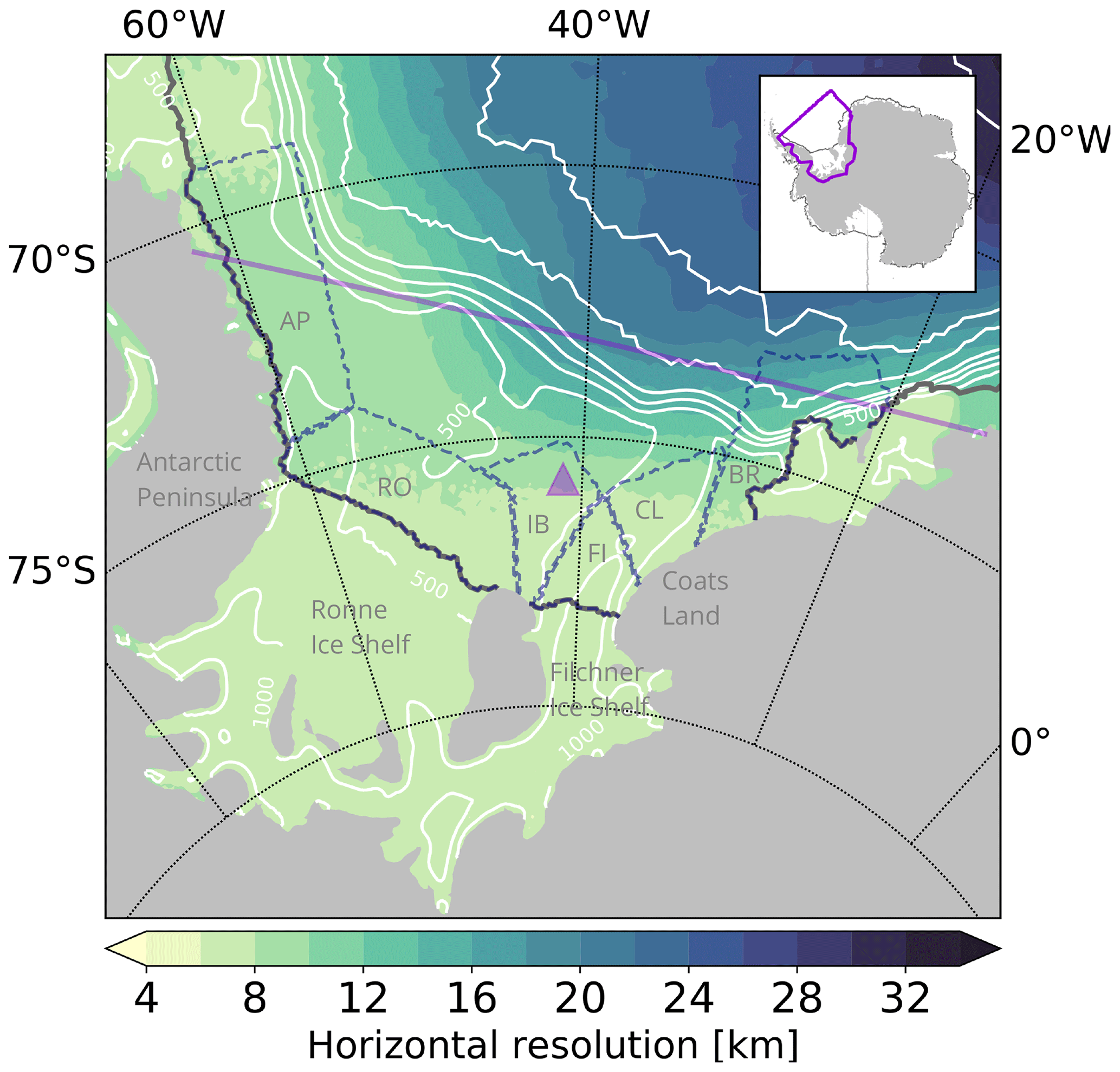
Figure 1 Horizontal resolution (km) over the Weddell Sea sector for the FESOM simulations. The ice shelf edge is contoured in gray, and isobaths are in white. The southern Weddell Sea control region is bounded to the north by the violet line following Drucker et al. (2011). The six sub-regions for comparison of polynya ice production (adapted from Paul et al., 2015) are enclosed by dashed gray lines: Antarctic Peninsula (AP), Ronne Ice Shelf (RO), the area around the ice mélange (IB), Filchner Ice Shelf (FI), Coats Land (CL) and Brunt Ice Shelf (BR). The location of the grounded iceberg A23-A for 2002–2017 is marked by a triangle (data from the Antarctic Iceberg Tracking Database; https://www.scp.byu.edu/data/iceberg/database1.html, last access: 22 March 2023; Budge and Long, 2018).

In a modeling study of the Filchner Ice Shelf system, Grosfeld et al. (2001) show that basal melt of the Filchner Ice Shelf decreases in the presence of grounded icebergs in front of it due to the weakened circulation within the ice shelf cavity. Studies in other regions have found that the representation of stationary features in the icescape (i.e., grounded icebergs, ice tongues, fast ice) can influence sea ice production and, consequently, ocean properties and basal melt. In a modeling study of the Amundsen continental shelf, Nakayama et al. (2014) found reduced sea ice export and sea ice formation in the Pine Island polynya in the presence of grounded icebergs west of it. Studies of the Mertz Glacier Tongue (MGT), East Antarctica, showed a drastic decrease in the sea ice production and dense water formation after a major calving event in 2010 (Kusahara et al., 2010, 2011), with consequences for the basal melt (Kusahara et al., 2017; Cougnon et al., 2017).

To simulate the surface freshwater flux in the southern Weddell Sea, we use a sea ice–ice shelf–ocean model with a regionally downscaled atmospheric forcing while also including effects of the ice mélange that was forming between FRIS and A23-A. We conduct sensitivity experiments using a coarser reanalysis product as atmospheric forcing and an experiment without the representation of the icescape. Based on these, we investigate the impact of both the regional atmospheric forcing and the icescape on the surface freshwater flux, the production rate and properties of the HSSW formed on the continental shelf, and the basal melt of FRIS.

2 Numerical model and experiments

2.1 Sea ice–ice shelf–ocean model

We use the global Finite Element Sea ice–ice shelf–Ocean Model (FESOM; Wang et al., 2014). Details of its dynamic–thermodynamic sea ice component are described by Timmermann et al. (2009) and Danilov et al. (2015), while the ice shelf component is described by Timmermann et al. (2012). The model has been found suitable for studies of the Southern Ocean ice–ocean–ice shelf systems (Timmermann et al., 2012; Timmermann and Hellmer, 2013; Nakayama et al., 2014). The net surface freshwater flux at the open ocean surface in the model comprises atmospheric fluxes (precipitation and evaporation), sea ice growth and melt, snowmelt fluxes, and the melt flux from the ice shelf base.

While precipitation (P) and evaporation (E) are given by the atmospheric forcing, other fluxes are calculated by the sea ice and ice shelf model. The freshwater flux F_i due to freezing/melting of ice and melting of snow is calculated as

$$\begin{array}{}\text{(1)}& {\displaystyle }{F}_{\text{i}}={\displaystyle \frac{(S_{\text{ref}}-S_{\text{i}})}{S_{\text{ref}}}}{\displaystyle \frac{{\mathit{\rho }}_{\text{i}}}{{\mathit{\rho }}_{\text{w}}}}{\displaystyle \frac{\partial h_{\text{i}}}{\partial t}}+{\displaystyle \frac{{\mathit{\rho }}_{\text{s}}}{{\mathit{\rho }}_{\text{w}}}}{\displaystyle \frac{\partial h_{\text{s}}}{\partial t}},\end{array}$$

where h_i and h_s are ice and snow thickness, respectively. The changes in sea ice and snow thickness, $\frac{\partial h_{\text{i}}}{\partial t}$ and $\frac{\partial h_{\text{s}}}{\partial t}$, are calculated by the sea ice model following Parkinson and Washington (1979) thermodynamics. Sea ice salinity S_i is assumed to be 5 psu. The reference salinity S_ref used for conversion between the freshwater and salt fluxes is taken to be the local time-evolving ocean surface salinity. The density of sea ice is ρ_i=910 kg m⁻³, and the density of snow ρ_s=290 kg m⁻³.

The freshwater flux in the open-water part of grid cell F_w depends on the air temperature (T_a) and percentage of the grid covered by ice (A) in the following way.

$$\begin{array}{}\text{(2)}& F_{\text{w}}=\left\{\begin{array}{ll}P-E& T_{\text{a}}\ge \mathrm{0}{}^{\circ }\text{C}\\ (\mathrm{1}-A)(P-E)& T_{\text{a}}<\mathrm{0}{}^{\circ }\text{C}.\end{array}\right.\end{array}$$

If the air temperature is above the freezing point of freshwater (T_a≥0 ^∘C), the net atmospheric flux P–E is applied directly to the ocean. For the temperatures below the freezing point, only the fraction 1−A of the net atmospheric flux is applied to the ocean, while the rest is accumulated as snow on the ice-covered part. The resulting freshwater flux F calculated by the sea ice model is a sum:

$$\begin{array}{}\text{(3)}& F=F_{\text{i}}+F_{\text{w}}.\end{array}$$

The impact of the net freshwater flux on ocean salinity is parameterized using a virtual salt flux formulation with the local time-evolving ocean surface salinity as reference salinity. The resulting salt flux is applied to the ocean model surface nodes and redistributed using a combination of k-profile parameterization (KPP; Large et al., 1994) and salt plume parameterization (Nguyen et al., 2009).

The elastic–viscous–plastic rheology (Hunke and Dukowicz, 1997) is used for computation of ice and snow drift, while sea surface tilt force is computed as a function of the sea surface height from the ocean model.

The horizontal grid resolution varies between 3 km under the Weddell Sea ice shelves and up to 25 km off the continental shelf in the Weddell Sea and increases to a maximum of 250 km in the Atlantic and Pacific oceans (Fig. 1). With a resolution of between 3–12 km in the region of interest, the model is not eddy-resolving, but circulation snapshots indicate that it is eddy-permitting. We use a hybrid vertical coordinate system with 36 layers. Terrain-following (sigma) coordinates are used for the sector shallower than 2500 m around Antarctica, while in the rest of the ocean we apply the z-level discretization. Ice shelf draft, cavity geometry and global ocean bathymetry have been prepared from the 1 min version of RTopo-2 (Schaffer et al., 2016).

2.2 Experimental design

The model was initialized in 1979 from temperature and salinity derived from the World Ocean Atlas 2009 data (Levitus et al., 2010) and run until the end of 2001 using atmospheric forcing from the ERA-Interim reanalysis (ERA; Dee et al., 2011) on a 75 km horizontal grid, with 6-hourly air temperature and dew-point temperature both at 2 m altitude and wind fields at 10 m altitude, as well as 12-hourly average shortwave and longwave radiation, precipitation, and evaporation. From this state, we extend the reference experiment (BRIDGE) until the end of 2017 using regionally downscaled forcing from the regional atmosphere model with 14 km horizontal resolution and, where available, incorporating effects of the grounded iceberg and the ice bridge as described below. To investigate the impact of the icescape, we conducted a sensitivity experiment without prescribing the blocking effect (i.e., blocking the movement of sea ice) of the varying icescape (noBRIDGE). An additional experiment (cATMO) without the blocking effect and using ERA as an atmospheric forcing everywhere was conducted to investigate the impact of the high-resolution atmospheric forcing used in the reference experiment. Both sensitivity experiments were initialized from the same conditions as BRIDGE and run for the same period, 2002–2017 (Table 1). Another 3-year simulation was extended from the conditions of the BRIDGE experiment at the end of 2014, with the same setup as BRIDGE except with the fixed fast-ice conditions (statBRIDGE).

Table 1 Experimental design.

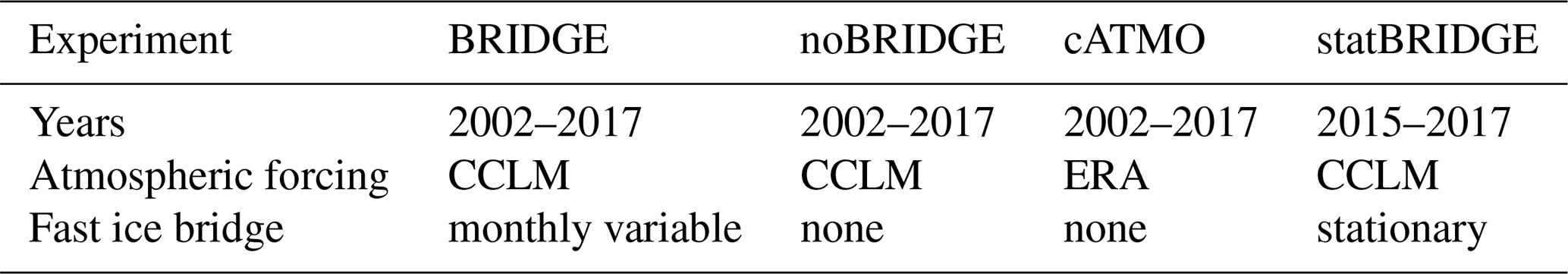
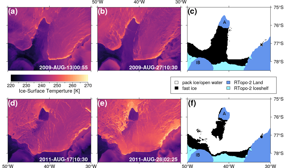
Figure 2 Comparison of the ice-surface temperatures from several single MODIS swaths from August 2009 (a, b) and August 2011 (d, e) and the derived fast-ice masks (c, f) with added marks for Berkner Island (IB) and grounded iceberg A23-A (A). Antarctic ice shelves and land configuration are based on RTopo-2 (Schaffer et al., 2016).

2.3 Ice mélange

A striking feature in the southern Weddell Sea icescape (2002–2017) is the ice mélange forming between Berkner Island and the grounded iceberg A23-A (Fig. 2). The iceberg A23-A broke off from the Filchner Ice Shelf in 1986. It had stayed grounded in the region since 1991. The iceberg started moving again in 2020, and ultimately, since the beginning of 2022, it has been moving out of the region (iceberg locations from the Antarctic Iceberg Data, USNIC, https://usicecenter.gov/Products/AntarcIcebergs, last access: 15 August 2023; Antarctic Iceberg Tracking Database, https://www.scp.byu.edu/data/iceberg/database1.html, last access: 22 March 2023, Budge and Long, 2018). As shown in Fig. 2a and b, higher temperatures associated with leads and polynya openings are detected in MODIS ice-surface temperature retrievals west of the iceberg A23-A and Berkner Island and in front of the Filchner Ice Shelf. The persistent absence of cracks, leads or polynyas in a well-defined area indicates stationary sea ice conditions between Berkner Island and iceberg A23-A in August 2009. In contrast, in August 2011, leads and polynyas can be found in the same area (Fig. 2d, e). A similar pattern of leads forming with a high frequency west of Berkner Island and A23-A and low frequency between the tip of Berkner Island and A23-A has been reported from the long-term (2003–2019) data derived from the thermal-infrared satellite measurements (Reiser et al., 2019).

Smaller icebergs, bergy bits, and accumulation of platelet ice (Hoppmann et al., 2020) are possible processes responsible for the formation of the ice bridge. These processes are subject to variability and are not represented in the current sea ice–ocean models, including FESOM. With the use of MODIS ice-surface temperature data (Hall and Riggs, 2015), we are able to get information about the existence, location and extent of the ice bridge. We use daily median ice-surface temperature from the cloud-corrected data (Paul et al., 2015) for April–September 2002–2017. We calculate daily temperature anomalies by subtracting the spatially averaged ice-surface temperature from each daily composite. Subsequently, for each month, the median of the ice-surface temperature anomaly is calculated per pixel from all daily anomalies. Under the assumption that persistent and immobile sea ice cover leads to lower-than-average monthly median temperature, negative values of anomalies exceeding amplitudes of 3 K are used to define the monthly fast-ice locations, meaning that, for example, in 2009 the ice bridge extended between A23-A and Berkner Island, whereas in 2011, the fast ice did not extend over the entire distance (Figs. 2c, f and 6). The fast-ice locations are mapped on the FESOM grid using the nearest-neighbor approach. We prescribe zero sea ice velocities in the so-defined fast-ice areas between Berkner Island and the grounded iceberg A23-A (between 35 and 45^∘ W) to simulate the blocking of the sea ice drift in BRIDGE. In noBRIDGE and cATMO, we impose no restrictions on the ice movement to simulate the conditions without the ice mélange.

2.4 Regional atmospheric forcing

In a model study for 2007–2009, Haid et al. (2015) found ice production in the southern Weddell Sea polynyas to be sensitive to the atmospheric forcing, with ice production increasing with increasing winds. We employ data from a regional atmospheric model to incorporate the impact of a regionally downscaled atmospheric forcing on the surface freshwater flux of the southern Weddell Sea. Atmospheric simulations over the Weddell Sea were performed using the non-hydrostatic atmospheric model COSMO-CLM (CCLM; Rockel et al., 2008; Steger and Bucchignani, 2020) as described by Zentek and Heinemann (2020). CCLM was adapted for polar conditions using a thermodynamic sea ice module (Schröder et al., 2011; Heinemann et al., 2021) with snow cover and a temperature-dependent albedo scheme (Gutjahr et al., 2016). Topography was derived from RTopo-2 (Schaffer et al., 2016), while ERA-Interim data were used for the initial and boundary conditions. Daily sea ice concentrations were taken from the satellite measurements (AMSR-E, SSMI/S, AMSR2; Spreen et al., 2008) to allow for a more realistic polynya representation. Here we use daily simulations performed with a 6 h spin-up time and 0.125^∘ (13.9 km) resolution for the period 2002–2017. In the experiments BRIDGE and noBRIDGE, we apply CCLM as a forcing over the Weddell Sea, whereas, consistent with the CCLM boundary conditions, ERA is used in other regions. In a zone surrounding the boundaries of the Weddell Sea and extending over 2^∘, we combine the two forcings using bilinear interpolation to ensure a smooth transition.

CCLM was validated with observations and compared to reanalyses by Zentek and Heinemann (2020). A comparison of CCLM for 1 year with measurements over the sea ice of the Weddell Sea shows small biases for temperature and wind speed (around ±1 ^∘C and 1 m s⁻¹, respectively). With the higher resolution of the CCLM forcing, katabatic winds and heat fluxes in polynyas are better resolved than in the case of the coarser reanalysis products. CCLM improves the representation of atmospheric features in topographically structured terrain (such as increased katabatic winds) when compared to ERA and has a more realistic thermal structure over coastal polynyas, which are not represented in ERA (Zentek and Heinemann, 2020). ERA has 2 ^∘C warmer air temperatures over most of the Weddell Sea, while it is 0.5 ^∘C cooler in narrow regions along the FRIS calving front and 2 ^∘C cooler along the eastern shelves (Fig. 3b). The higher temperatures (up to 3 ^∘C) in ERA, when compared to CCLM, are also found in the grounded iceberg A23-A area, as the grounded iceberg is treated as land ice in CCLM. A warm bias of ERA has been found in several other studies and is caused by the missing snow layer in the ERA sea ice parameterization (Batrak and Müller, 2019; Heinemann et al., 2022). Both ERA and CCLM exhibit wind maxima in the southwestern corner between the Antarctic Peninsula and Ronne Ice Shelf and next to the Brunt Ice Shelf (Fig. 3c and d). The latter is related to katabatic winds from Coats Land, while the former is associated with barrier winds along the Antarctic Peninsula (Heinemann and Zentek, 2021). However, another maximum north of Berkner Island is present in the CCLM data, suggesting that the higher horizontal resolution of the CCLM model allows for a more realistic representation of the off-shore winds guided by topography along Berkner Island (see Heinemann and Zentek, 2021). The most pronounced differences between the wind fields are weaker winds over the eastern ice shelves and a stronger maximum off the Ronne Ice Shelf in CCLM (Fig. 3b). Minor differences in the precipitation and evaporation between the two data sets are limited to the outer Weddell Sea (not shown).

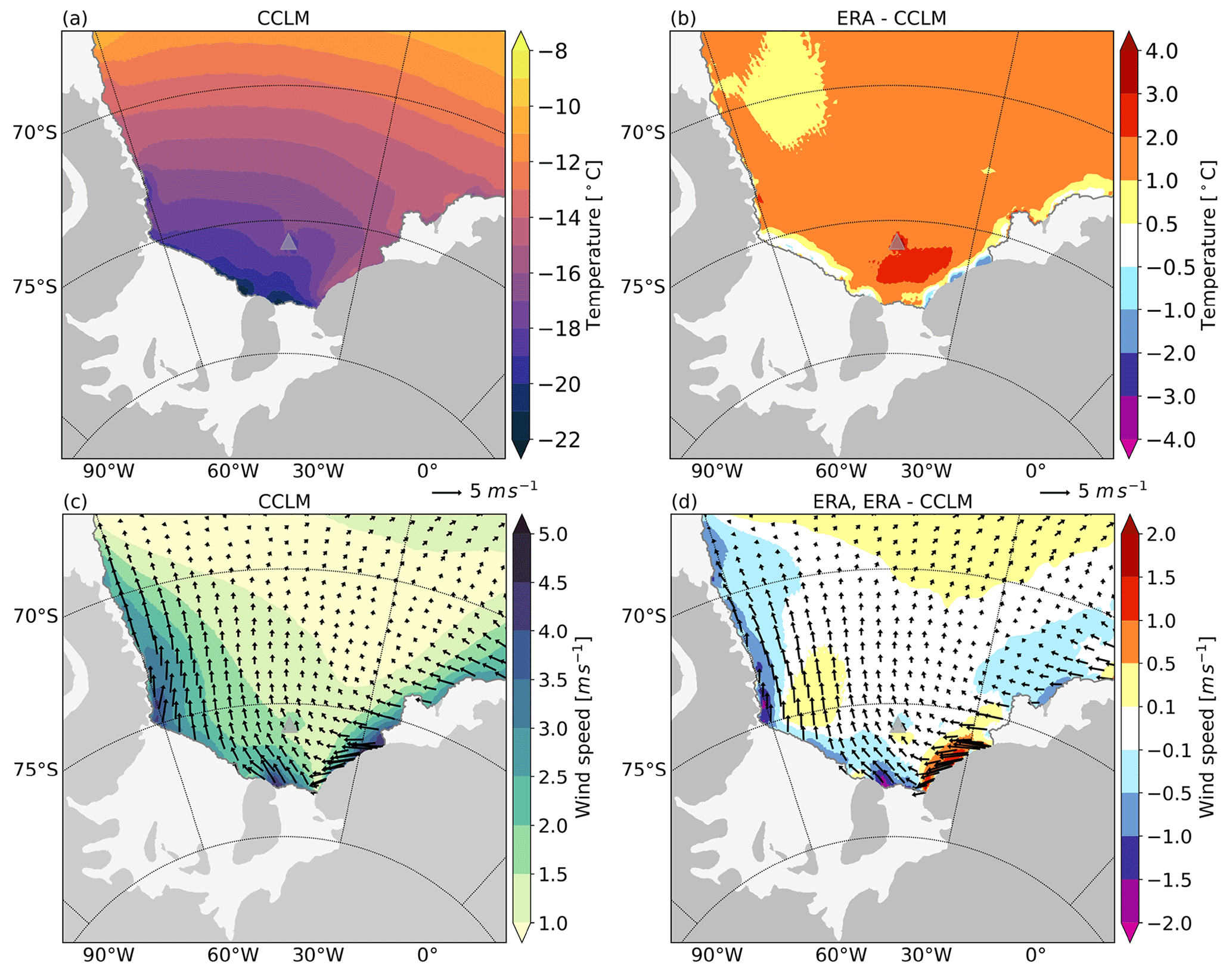
Figure 3 (a) Mean air temperature (2002–2017) from CCLM and (b) air temperature difference between ERA-Interim and CCLM. (c) Mean wind field (2002–2017) from CCLM and (d) ERA-Interim, with wind speed difference between ERA-Interim and CCLM. Data are shown only over the ocean. The Antarctic continent is drawn in gray; ice shelves are marked in light gray. The location of the grounded iceberg A23-A (2002–2017) is marked by a triangle.

3 Results and discussion

3.1 Reference experiment

3.1.1 Surface freshwater flux

In the Weddell Sea, there is a clear separation between the negative and positive net surface freshwater flux regions, corresponding to areas where sea ice growth dominates melt and vice versa. Corresponding to freshwater removal by sea ice growth, we find a negative flux with values between −2 and −1 m a⁻¹ over most of the continental shelf (Fig. 4a). In front of the Filchner Ice Shelf and in the region west of the ice mélange, surface freshwater flux reaches −5 m a⁻¹, while in a narrow band adjacent to the Ronne and Brunt ice shelves, it reaches −12 m a⁻¹. These are also the locations with the highest occurrence of polynyas, defined here as nodes with simulated ice growth for which ice concentration is smaller than 70 %, or ice thickness is smaller than 20 cm. Given that the strong ocean-to-atmosphere heat fluxes in polynyas occur over both the open ocean and thin ice areas, these criteria have been widely used in other studies (e.g., Haid and Timmermann, 2013; Haid et al., 2015 or Nihashi and Ohshima, 2015a; Paul et al., 2015). The geographical pattern of polynyas (Fig. 4b) is overall similar to the one from Paul et al. (2015) and includes major polynyas detected in other satellite-based studies (e.g., Drucker et al., 2011; Nihashi and Ohshima, 2015a). The details of sea ice production within polynyas are discussed in Sect. 3.1.2. In the seasonally ice-covered zone, the positive freshwater flux related to the sea ice melt is the strongest along the sea ice margins (up to 1.5 m a⁻¹, not shown). Patterns of positive freshwater flux (up to 2 m a⁻¹) can also be found at the continental shelf break, where the vertical entrainment of Warm Deep Water into the surface mixed layer drives basal melting. Paul et al. (2015) noted the high occurrence of thin ice in this region, as one of the few regions where thin ice was detected out of the coastal polynyas.

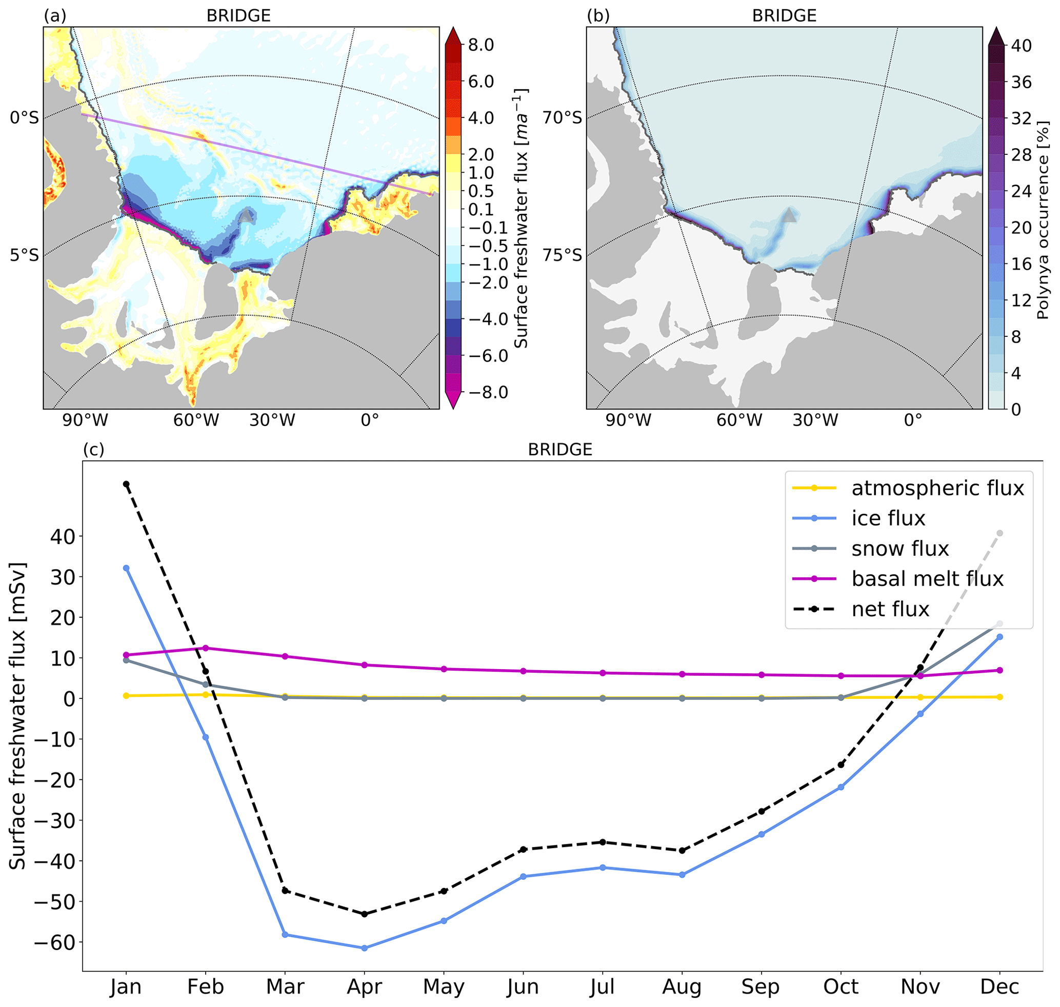
Figure 4 (a) Annual mean net surface freshwater flux (2002–2017) from BRIDGE, with positive values corresponding to a flux in the ocean. The southern Weddell Sea control region is enclosed by the violet line. Note that the color map does not linearly scale with the data. (b) Annual mean occurrence of polynyas (2002–2017) calculated as a percentage of days in the year with sea ice production occurring at nodes with ice concentration <70 % or ice thickness <20 cm. The location of the grounded iceberg A23-A (2002–2017) is marked by a triangle. (c) Monthly mean surface freshwater fluxes (2002–2017) from BRIDGE for the southern Weddell Sea control region.

Under the ice shelves, positive freshwater flux is due to basal melt and negative due to freezing at the ice shelf base. The overall pattern of the basal melt under FRIS is similar to the satellite data (Rignot et al., 2013; Moholdt et al., 2014; Adusumilli et al., 2020). The freshwater input is the strongest near the grounding lines (up to 3 m a⁻¹) and more moderate at the ice fronts (Fig. 4a). Moderate freezing (−1 m a⁻¹) is found at the Ronne Ice Shelf center and along its western edge, as well as on the eastern side of Berkner Island and under the northeastern Filchner Ice Shelf. The eastern edge of the Filchner Ice Shelf is dominated by basal melt similar to in Rignot et al. (2013). In the southern Filchner Ice Shelf, we find a band of basal melt rates reaching 2 m a⁻¹, which is missing in the satellite-based estimates (Rignot et al., 2013). Data from repeated radar measurements (Zeising et al., 2022) show indeed locally enhanced basal melt in this region, albeit with a weaker amplitude (1.13 m a⁻¹) than in BRIDGE. Compared to Adusumilli et al. (2020), a stronger melt and weaker freezing signal is found in BRIDGE in the northeastern Filchner cavity. The difference could result from the too-strong HSSW inflow in the Filchner cavity in BRIDGE.

The strength of the melting and freezing maxima in BRIDGE is weaker than in the satellite-based estimates from Moholdt et al. (2014). The absence of tides in our model could be a possible explanation for this difference, as they enhance both the basal melt and refreezing due to the increased mixing (Hausmann et al., 2020). However, changes in the basal melt related to changes in the surface freshwater flux on the continental shelf are primarily density-driven (Nicholls and Østerhus, 2004; Hattermann et al., 2021). Therefore, the lack of tides in our model does not affect the conclusions of this study.

The seasonal evolution of the net surface freshwater flux and its components for the continental shelf of the southern Weddell Sea is shown in Fig. 4c. The seasonal cycle of the net freshwater flux (2002–2017) is dominated by ice growth and melt fluxes: it is negative in March–October due to the effect of sea ice production and positive in November–February due to the effect of the combined ice melt and snowmelt. The annual mean net flux is −16.3 mSv (1 mSv = 1000 m³s⁻¹), as the extraction of freshwater due to ice production dominates the sum of fluxes. P–E provides a mean freshwater input of 0.3 mSv, and the melting of snow is 3.1 mSv. The ice shelf basal melt flux provides another 7.6 mSv, out of which 5.2 mSv originates from FRIS. Converted to gigatonnes per year using an ice density of 910 kg m⁻³, this corresponds to 150.9 Gt a⁻¹, which falls in the range of the satellite-based estimates from Moholdt et al. (2014) (58–190 Gt a⁻¹), Rignot et al. (2013) (110–200 Gt a⁻¹) and Adusumilli et al. (2020) (81.4 ± 122.9 Gt a⁻¹).

The melting of icebergs can be another source of freshwater; however, this flux is not included in our model. Based on the iceberg melt climatology from Rackow et al. (2017), magnitudes of the iceberg melt rates on the southern Weddell Sea continental shelf are low (around 0.3 m a⁻¹) compared to the magnitudes of the sea ice fluxes. Freshwater flux from the iceberg melt, therefore, would have a relatively small impact on the surface freshwater flux in the region when compared to the dominant sea ice fluxes.

The sea ice export out of the southern Weddell Sea is the main reason for the imbalance between the ice production and melt fluxes. On average (2002–2017), 1509 km³ a⁻¹ of ice is produced on the southern Weddell Sea continental shelf in BRIDGE. With the net sea ice export of 1041 km³ a⁻¹, 70 % of the produced ice is exported from the region. The mean net sea ice export across the 69.5^∘ S latitude band (2002–2017) in BRIDGE is 1567 km³ a⁻¹ (38 mSv). Across the same latitude, Haumann et al. (2016) estimated long-term annual freshwater flux due to the northward sea ice transport across the 69.5^∘ S in the Weddell Sea to be 50 ± 20 mSv. Based on passive microwave data, Drucker et al. (2011) calculated the net export of sea ice area out of the southern Weddell Sea (April–October 2003–2008) and found it to be 5.2×10⁵ km²a⁻¹. We find the net sea ice area export, across approximately the same gates and for the same time, in BRIDGE to be 5.1×10⁵ km²a⁻¹, quite close to the observed estimates, with a corresponding net sea ice volume export of 814 km³ a⁻¹.

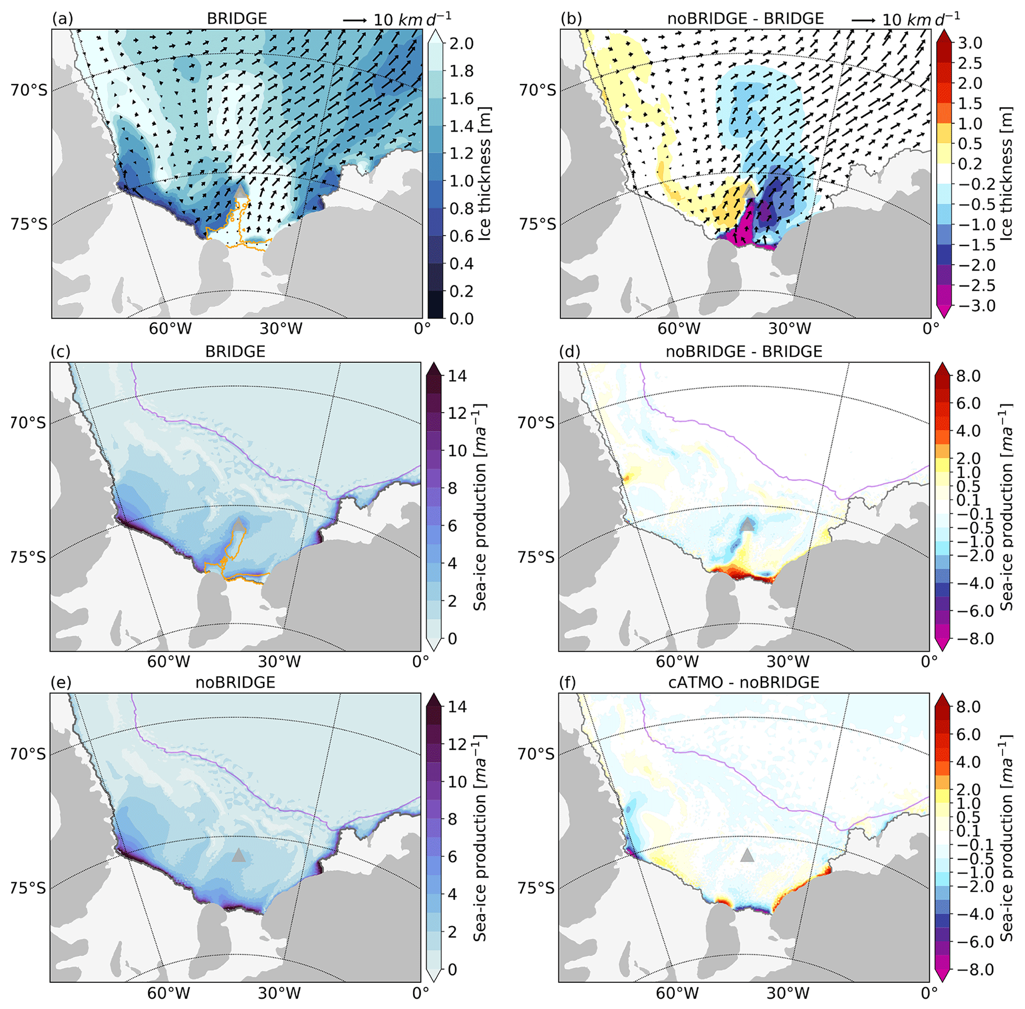
Figure 5 (a) Sea ice thickness and velocity from BRIDGE in August 2009, when the ice bridge was fully formed based on the monthly satellite data (Fig. 2c) and (b) thickness difference between noBRIDGE and BRIDGE, with the velocity from noBRIDGE in August 2009. (c) Mean sea ice growth rates (2002–2017) from BRIDGE and (d) difference between noBRIDGE and BRIDGE. (e) Mean sea ice growth rates (2002–2017) from noBRIDGE and (f) difference between cATMO and noBRIDGE. The location of the grounded iceberg A23-A (2002–2017) is marked by a triangle. The average fast-ice area in (a) and (c) is indicated by an orange contour. The 2500 m isobath is indicated by a violet contour. Note that the color map does not linearly scale with the data in (b), (d) and (f).

Drucker et al. (2011)Nihashi and Ohshima (2015a)Tamura and Ohshima (2011)Nihashi and Ohshima (2015a)Paul et al. (2015)Haid and Timmermann (2013)

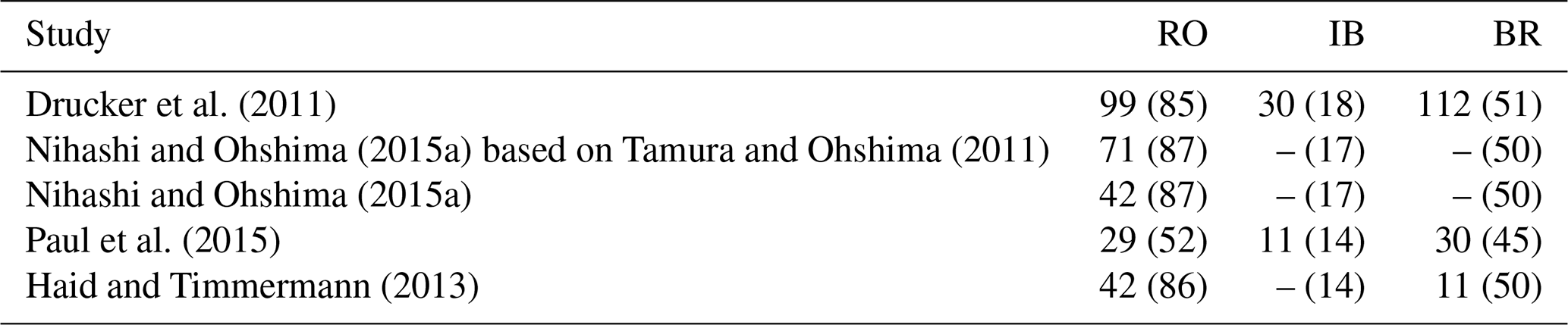
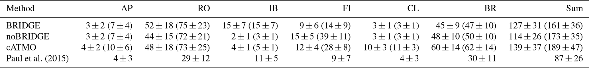
Table 2 Summary of cumulative polynya-based ice production (km³) for freezing season from various studies, with the corresponding values from BRIDGE in parentheses.

3.1.2 Sea ice production

The pattern of the negative surface freshwater flux in BRIDGE (Fig. 4a) corresponds to the pattern of the annual mean sea ice production in Fig. 5c. A belt of elevated sea ice production rates is found in the coastal polynyas along the ice shelf fronts and coastlines, with maximum values up to 15 m a⁻¹ in the corner between the Antarctic Peninsula and the Ronne Ice Shelf and west of the Brunt Ice Shelf. Strong sea ice production rates also occur west of the ice mélange associated with the grounded iceberg A23-A. To estimate the role of polynyas in the surface freshwater flux of the southern Weddell Sea, we calculate cumulative annual ice production both within and outside polynyas from the daily model output (only positive growth rates are considered). The sea ice production occurring at the nodes where the sea ice concentration is smaller than 70 %, or thickness is smaller than 20 cm, is counted as polynya-based ice production. Although thus-defined polynyas cover only 2 % of the southern Weddell Sea area, their higher average ice growth rate (20 m a⁻¹) compared to outside polynyas (4 m a⁻¹) significantly contributes to the total ice production in the region.

For 2002–2017, 17 % (260 km³ a⁻¹) of the ice produced on the continental shelf of the southern Weddell Sea (1509 km³ a⁻¹) comes from polynyas in BRIDGE. To investigate the regional distribution and compare the simulated polynya ice production with other studies, we divided the continental shelf into six sub-regions (Fig. 1) adapted from Paul et al. (2015) by extending them to the coastline in the model. The largest annual ice production in BRIDGE is found in the Ronne (RO; 123 km³ a⁻¹) and Brunt (BR; 79 km³ a⁻¹) ice shelves regions. At the same time, significant ice production can also be found in the region associated with the ice bridge (IB; 20 km³ a⁻¹) and in front of the Filchner Ice Shelf (FI; 27 km³ a⁻¹).

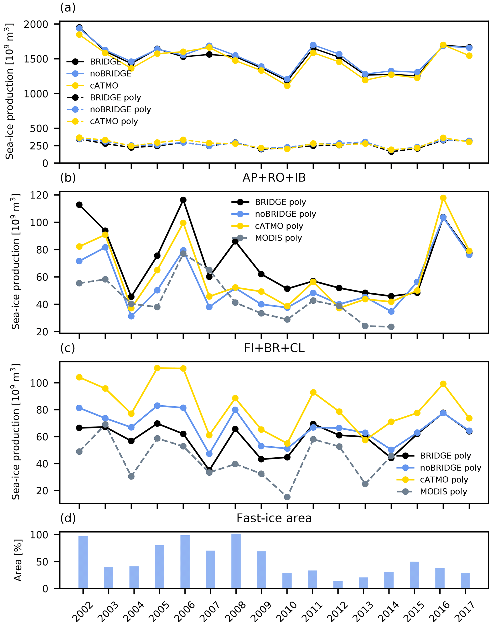
Figure 6 (a) Time series of the total and polynya-only annual cumulative ice production (2002–2017) in the southern Weddell Sea from FESOM experiments. (b) Time series of the April–September 2002–2017 polynya ice production from FESOM and the MODIS-based estimates for AP, RO and IB sub-regions from Paul et al. (2015). (c) Time series of the April–September 2002–2017 polynya ice production from FESOM and the MODIS-based estimates for FI, BR and CL sub-regions from Paul et al. (2015). (d) Time series (2002–2017) of the average annual fast-ice area in the BRIDGE experiment (as a percentage of the maximum in 2008).

Comparing different estimates of the ice production within polynyas is difficult, as different methods (i.e., heat flux parameterizations and atmospheric forcing, treatment of fast ice) and differences in regional and seasonal coverage lead to a large spread between the studies. Since ice production in polynyas exhibits a large interannual variability (Fig. 6) and depends on the length of the season taken into account, we aim to match the sampling periods and areas from the other studies in the best possible way (Table 2). Drucker et al. (2011) report mean ice production of 99 km³ a⁻¹ for the Ronne and 112 km³ a⁻¹ for the Brunt region (April–October 2003–2008). The corresponding values for similar regions from BRIDGE are smaller, and the Ronne (RO) ice production (85 km³ a⁻¹) in our case is higher than the Brunt (BR) ice production (51 km³ a⁻¹). They also report significant ice production (30 km³ a⁻¹) in polynyas associated with the grounded iceberg A23-A. For the corresponding period, 18 km³ a⁻¹ of ice is produced in polynyas forming west of the ice mélange between Berkner Island and A23-A in BRIDGE. For March–October 2003–2007, Nihashi and Ohshima (2015a) report 42 km³ a⁻¹ of ice produced in the Ronne polynya. For the same period and a similar area (RO), we find polynya ice production in BRIDGE to be much larger, 87 km³ a⁻¹. In the narrow region along the Ronne Ice Shelf, where the ice growth rates in the model are particularly high, Nihashi and Ohshima (2015a) detected fast ice, not polynyas. They found that discrimination of fast ice from the polynya areas in the satellite data reduces the sea ice production estimates. Based on the coarser data without the fast-ice mask, Tamura and Ohshima (2011) reported ice production of 71 km³ a⁻¹ for the Ronne region (for the corresponding period), which is much closer to our results. As the fast ice from this region is not included in our model, this likely contributes to the discrepancy between our results and Nihashi and Ohshima (2015a).

The most detailed estimates of the regional polynya ice production are found in Paul et al. (2015) (April–September 2002–2014). The regional distribution of the ice production in BRIDGE is very similar to the one found by Paul et al. (2015) (Table 3). Their estimates for RO (29 km³ a⁻¹), BR (30 km³ a⁻¹) and FI (9 km³ a⁻¹) are smaller than the corresponding results from BRIDGE (75, 47 and 14 km³ a⁻¹, respectively), while there is good agreement with simulated ice production for another significant polynya ice production region, IB (11 km³ a⁻¹ compared to 15 km³ a⁻¹ in BRIDGE). The data from Paul et al. (2015) incorporate a different land mask from that in our model, with differences being the largest for RO and FI. Integrating results from BRIDGE over the same area as in Paul et al. (2015) yields 52 km³ a⁻¹ for RO and 9 km³a⁻¹ for FI. It should be noted that the warm bias of the ERA data used in the MODIS retrieval tends to reduce polynya area and ice production, possibly explaining the smaller values in Paul et al. (2015). Furthermore, we find that on average only 64 % (167 km³ a⁻¹ out of 260 km³ a⁻¹) of ice in the southern Weddell Sea polynyas is produced over the season covered by the satellite data (April–September), meaning that a non-negligible ice production is not covered by the satellite-based estimates.

In an earlier FESOM study, Haid and Timmermann (2013) found the contribution from Ronne to be 42 km³ a⁻¹, from Brunt to be 11 km³ a⁻¹ and from the Antarctic Peninsula region to be 19 km³ a⁻¹ (May–September 2002–2009). We find ice production to be 86 km³ a⁻¹ for Ronne (RO), 50 km³ a⁻¹ for Brunt (BR) and only 8 km³ a⁻¹ in the Antarctic Peninsula region (AP) for the corresponding period. Furthermore, the grounded iceberg A23-A and the associated ice bridge were not represented in Haid and Timmermann (2013), where we find non-negligible polynya ice production of 18 km³ a⁻¹ for 2002–2009. Except for the representation of the ice bridge, the differences between our studies are likely further influenced by the different atmospheric forcing used in Haid and Timmermann (2013). However, the two model configurations also differ in other aspects (e.g., the representation of the ice shelf, topography, resolution).

Overall, the regional pattern of polynya ice production is well represented in BRIDGE when compared to the satellite-based studies, with the largest contributions from the Ronne (RO) and Brunt (BR) polynyas, followed by the Filchner (FI) polynya and polynyas associated with the ice bridge (IB). The strength of ice production in BRIDGE falls in the range of estimates from the satellite-based studies, albeit on the higher side. Differences in the land masks and representation of the fast ice are the likely reason of some of these differences.

3.2 Impact of the icescape on sea ice production

As shown in Fig. 2, the variable ice mélange between the coast and iceberg A23-A influences the sea ice distribution. A study investigating the influence of the icebergs grounded north of Berkner Island on sea ice conditions (Markus, 1996) reported significant ice concentration increase east of the grounded icebergs (in front of the Filchner Ice Shelf) due to their blocking of the clockwise sea ice drift. To mimic the blocking effect of the ice mélange on the sea ice drift, zero sea ice velocities in the areas identified by the MODIS data were prescribed in BRIDGE (Fig. 5a, c). We investigate the influence of the ice mélange on ice production by comparing the results of noBRIDGE (without the blocking effect) to BRIDGE.

Paul et al. (2015)

Table 3 Cumulative polynya-based ice production (km³) for April–September 2002–2014 from FESOM experiments and Paul et al. (2015) for six sub-regions defined in Paul et al. (2015). Values from the control regions shown in Fig. 1 for FESOM experiments are shown in parentheses.

Sea ice velocity and ice thickness from BRIDGE and noBRIDGE for August 2009, when the ice bridge was fully formed (Fig. 2c), are shown in Fig. 5a and b. In BRIDGE, east of the ice bridge, the ice gets thicker compared to noBRIDGE, while thinner ice can be found west of the ice bridge. Due to the shifted polynya development in noBRIDGE, mean (2002–2017) net sea ice growth rates are decreased west of the ice bridge and increased east of it (Fig. 5d). Accumulated ice production decreases most notably north of Berkner Island (IB) (from 20 km³ a⁻¹ in BRIDGE to 5 km³ a⁻¹ in noBRIDGE) and increases in front of Filchner Ice Shelf (FI) (from 27 to 58 km³ a⁻¹), where much thinner ice is found in noBRIDGE. Leaving out the impact of the ice bridge on sea ice formation in our simulations, thus, pushes sea ice formation in those regions further from the satellite-based estimates (Paul et al., 2015).

Changes in the icescape also modify the interannual sea ice production variability (Fig. 6). The differences between BRIDGE and noBRIDGE are most pronounced in the years when the ice bridge is fully formed; i.e., the fast-ice area is close to its maximum (2002, 2005–2010; Fig. 6d). Reduced ice bridge formation in 2015–2017 leads to a similar increase in sea ice production between the experiments, which can be attributed to the intensification of the southerly winds under the influence of the large-scale atmospheric forcing patterns (Hattermann et al., 2021). As the ice front position and landfast ice are strongly influenced by the offshore winds (Christie et al., 2022), episodic strengthening of southerly winds likely played a role in weakening the ice bridge.

3.3 Impact of the regional atmospheric forcing on sea ice production

In an earlier FESOM study, Haid et al. (2015) found ice production (2007–2009) in the southern Weddell Sea polynyas to be sensitive to the atmospheric forcing, with ice production increasing with increasing offshore winds. With the higher resolution of the CCLM forcing, topographically influenced winds and heat fluxes in polynyas are better resolved than in the case of ERA (see Heinemann and Zentek, 2021). Here we examine the influence of the regional and large-scale atmospheric forcing on sea ice production by comparing results of cATMO (forced by ERA) to noBRIDGE (forced by CCLM over the Weddell Sea sector). To ensure consistency with the CCLM boundary conditions and to exclude effects of differences in the large-scale atmospheric influences between the two experiments, ERA was used as a forcing across the entire model domain in cATMO and outside of the Weddell Sea region in the noBRIDGE experiment.

As the local offshore winds play a key role in the development of polynyas, the differences in the wind fields between the atmospheric forcings used in noBRIDGE and cATMO are reflected in the ice production fields (Fig. 5f). The most significant differences in the simulated polynya heat fluxes that determine the ice production are found for the sensible heat flux in locations with the strongest wind differences (not shown). The stronger winds from the Coats Land and along the Brunt Ice Shelf lead to stronger sea ice production rates in cATMO when compared to noBRIDGE. At the same time, in the Ronne corner and surrounding Berkner Island, where offshore winds are weaker in cATMO, sea ice production rates are reduced.

The mean ice production on the continental shelf in cATMO is smaller (1470 km³ a⁻¹) than in noBRIDGE (1535 km³ a⁻¹), and polynyas account for 19 % of the total ice production. Compared to noBRIDGE, annual polynya ice production in the Ronne region is slightly decreased in cATMO (RO, from to 114 to 111 km³ a⁻¹), while the most notable finding is increased polynya ice production for the Brunt region (BR, from 84 to 94 km³ a⁻¹). The increase in ice production in cATMO over the eastern shelves (CL and BR) takes ice production for those sub-regions (CL an BR) further from the estimates from Paul et al. (2015).

The interannual variability in the cumulative annual sea ice production for the southern Weddell Sea is shown in Fig. 6. In both experiments, sea ice production exhibits large interannual variability. For 2002–2017, we find polynya ice production to be 276 ± 53 km³ a⁻¹ in cATMO and similarly in noBRIDGE to be 270 ± 44 km³ a⁻¹. While the regional forcing does not significantly impact interannual variability of sea ice production outside polynyas, it modifies variability within the polynyas. In cATMO, annual polynya ice production and ice production outside polynyas (2002–2017) are highly correlated (r=0.85, p=0.001). In noBRIDGE, this correlation is weaker (r=0.74, p=0.003), indicating a stronger influence of the local rather than the large-scale forcing on the polynya-based ice production variability. The decreasing trend (2002–2017) for the polynya-based ice production in noBRIDGE (−1.4 km³ a⁻¹) is weaker than in cATMO (−3.3 km³ a⁻¹). However, both experiments show an increase in polynya ice production between 2015–2017. This increase has also been noted by Hattermann et al. (2021) based on the ERA-Interim data and attributed to the intensification of the southerly winds under the influence of the large-scale atmospheric circulation. As ERA is used as the atmospheric forcing in cATMO and as boundary conditions for the CCLM forcing in noBRIDGE and BRIDGE, these effects of the large-scale atmospheric forcing on sea ice production are also simulated in our experiments.

The multidecadal ice production decrease in the southern Weddell Sea, driven by northerly wind trend, has been reported by Zhou et al. (2023). They found a >40 % decline in the Ronne and Berkner Bank polynya ice production rate (1992–2020), possibly driving a 30 % reduction in Weddell Sea Bottom Water volume since 1992. Based on the combined results from the long ERA run (1979–2002) and cATMO (2002–2017), we find a decreasing trend of −6.2 km³ a⁻¹ (24 % reduction based on the linear trend estimate) for the total sea ice production (1992–2017) over the corresponding region (RO and IB) and −1.8 km³ a⁻¹ (28 % reduction based on the linear trend estimate) for the polynya-only ice production. As the estimate of sea ice formation trend from Zhou et al. (2023) is predominately a function of the sea ice concentration data used for the calculation of sea ice formation rate, the stronger decreasing trend in their study could be related to the relatively coarse sea ice concentration data (25 km gridded) that do not resolve polynyas well.

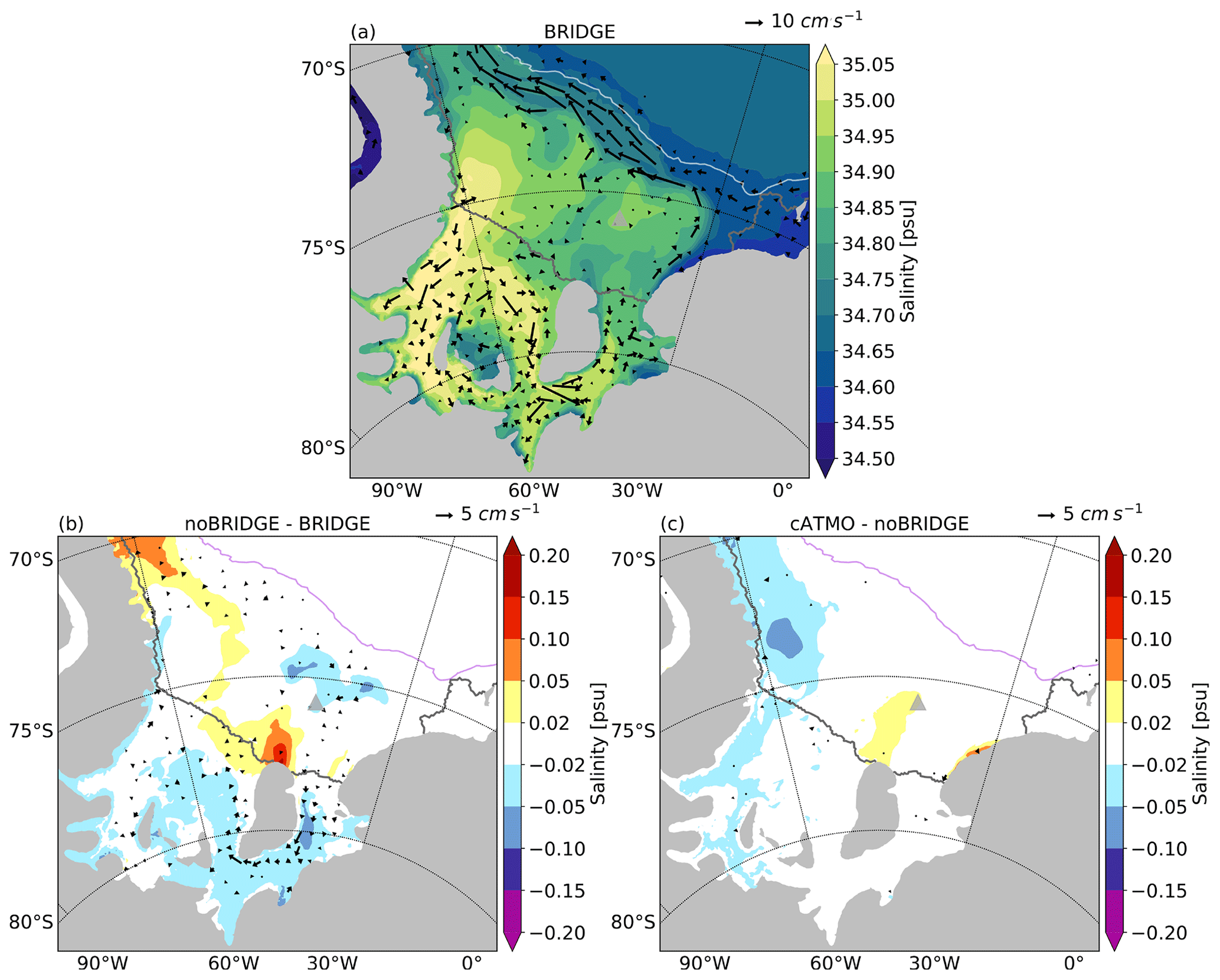
Figure 7 (a) Mean (2002–2017) bottom salinity and velocity from BRIDGE. The ice shelf edge is indicated by a gray contour, and the 2500 m isobath is marked by a white contour. Difference (2002–2017) in the mean bottom salinity and velocity between (b) noBRIDGE and BRIDGE and (c) cATMO and noBRIDGE (only mean velocities and velocity differences with magnitudes higher than 1 cms⁻¹ are shown). The ice shelf edge is indicated by a gray contour, and the 2500 m isobath is marked by a violet contour. The location of the grounded iceberg A23-A (2002–2017) is marked by a triangle in all panels.

3.4 HSSW formation

Dense shelf water with salinities S>34.6 psu is classified as HSSW and formed on the continental shelf of the southern Weddell Sea as a result of the salt enrichment through sea ice production. With temperatures near the freezing point, the density of HSSW depends primarily on the salt content. The signature of the HSSW can be found in the simulated mean bottom salinity field (2002–2017) along the southern Weddell Sea continental shelf, with the salinity increasing from the eastern to the western end of the shelf (Fig. 7a). The salinity maximum in BRIDGE corresponds to the main observed HSSW production site (Nicholls et al., 2009) at the corner between the front of the Ronne Ice Shelf and the Antarctic Peninsula (around 35 psu). Another maximum is found north of the ice bridge and grounded iceberg (around 34.9 psu). The mean bottom salinities at the Ronne ice front (34.85–35 psu) are higher than in the CTD (conductivity–temperature–depth) measurements from austral summer 2018 (around 34.8 psu) (Janout et al., 2021). Similarly, the salinity at the Filchner ice front (34.75–34.85 psu) is higher than in the latest observations (around 34.6 psu) (Janout et al., 2021). The simulated mean summer values are a bit smaller (34.85–34.9 psu) and closer to the observations at the Ronne ice front, while those at the Filchner ice front are still 0.1–0.15 psu saltier than the observations. In the summer 2018, the Filchner ice front was dominated by Ice Shelf Water (ISW) originating from the Ronne-sourced HSSW and modified in the interaction with the ice shelf base, which leads to smaller bottom salinities than in the presence of the more locally produced Berkner-sourced HSSW found at the Filchner ice front in, for example, 2017 (bottom salinities of 34.70–34.75 psu) (Janout et al., 2021). While being saltier than the observations, model results indicate prevalence of the locally produced HSSW on the Filchner ice front between 2002–2017.

Differences in the mean bottom salinity between the experiments (Fig. 7b, c) correspond to the sea ice production differences (Fig. 5). Without the presence of the ice bridge, saltier waters can be found north and northwest of Berkner Island, while less salty waters can be found north of the grounded iceberg. Corresponding to the location of the weaker sea ice production in cATMO compared to noBRIDGE, fresher water can be found in the Ronne corner and traced along the western edge of the Ronne cavity. North of Berkner Island, salinity in cATMO is slightly increased when compared to noBRIDGE, and saltier waters can also be found in a narrow band along the eastern ice shelves, following the sea ice production intensification in cATMO. Among all of the experiments, the least salty waters north of Berkner Island and Filchner Ice Shelf are found in BRIDGE, with values closer to the observations.

We calculated the mean production rate of HSSW on the southern Weddell Sea continental shelf from the net volume flux of HSSW in the region. The annual net flux is calculated from the daily data (2002–2017) over the temperature–salinity classes in the HSSW range (temperature of −1.9 to −1.5 ^∘C and salinity S>34.6 psu), with intervals of 0.05 psu for salinity and taking into account only the positive net values (the HSSW volume gain). It should be noted that the interaction of HSSW with the surrounding ice shelves beside FRIS is assumed to be negligible, while export of HSSW to the Ronne and Filchner cavity, as well as export across the northern bound of the region (Fig. 1), is accounted for. The mean production rate (2002–2017) in BRIDGE is 4.9 Sv, and it is slightly weaker in noBRIDGE (4.8 Sv), the strongest being in cATMO (5.0 Sv). Due to the too-high salinity in our experiments, particularly on the eastern side of the continental shelf, our estimate is likely an upper bound of the HSSW production magnitude. For comparison, based on observations Nicholls et al. (2009) estimated HSSW production on the southern Weddell Sea continental shelf to be 3 Sv. The mean HSSW production on the western continental shelf in BRIDGE is 3.2 Sv, while production rates in noBRIDGE and cATMO are weaker and similar (2.9 and 3.0 Sv). On the eastern shelf, the lowest production rate among the experiments is found in BRIDGE (1.7 Sv). The production rates from the sensitivity experiments without effects of the ice bridge are stronger and increase from noBRIDGE to cATMO (from 1.9 to 2 Sv). These results are consistent with the changes found in the hydrographic observations before and after the grounding of the icebergs in 1986. Changes in the icescape affected the local hydrography and caused the cessation of HSSW formation east of the grounded icebergs (Nøst and Østerhus, 1985).

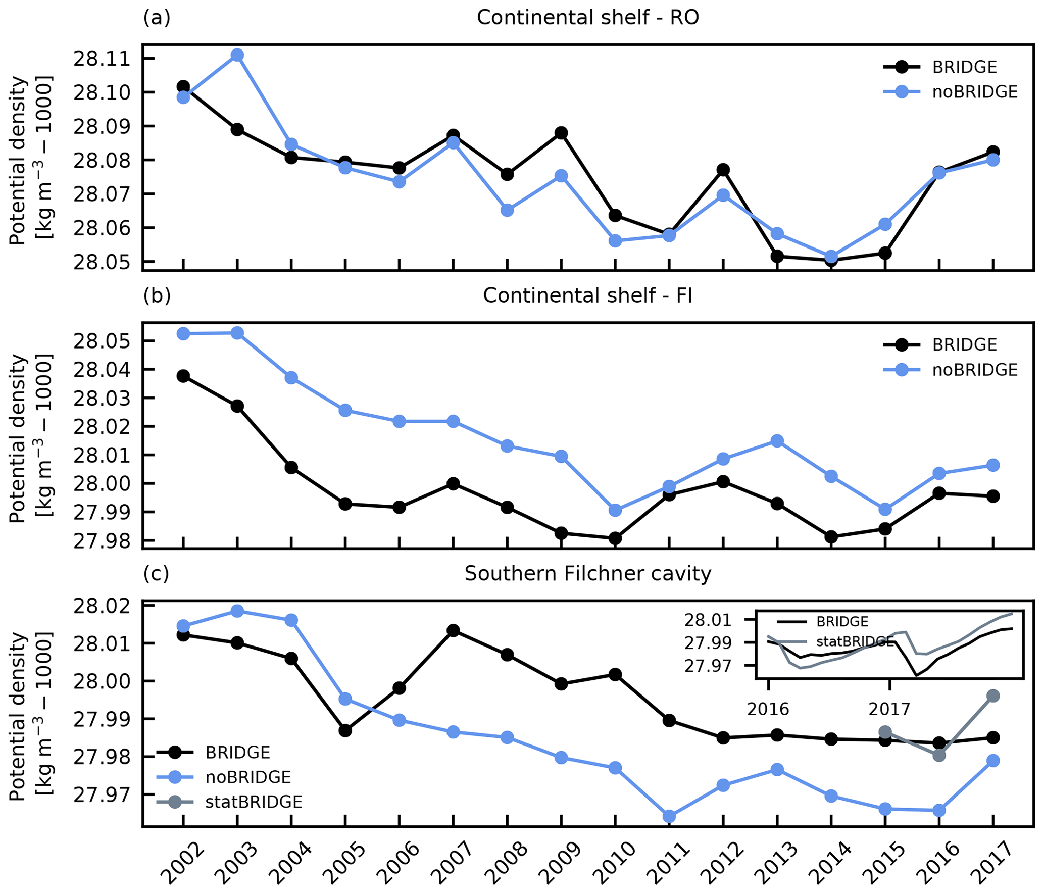
Figure 8 (a) Time series of the volume-averaged density on the (a) western (sub-region RO) and (b) eastern continental shelf (sub-region FI) and (c) within the southern Filchner cavity from the FESOM experiments.

3.5 Sub-ice shelf circulation

HSSW flows into the cavity and impacts the sub-ice shelf circulation. The bottom salinity and velocity (Fig. 7a) reveal the main pathways of the HSSW inflow in the cavity from the western continental shelf – along the western edge of the Ronne cavity through the Ronne Depression, along the western coast of Berkner Island and then to the rest of the cavity – while HSSW produced on the eastern part of the continental shelf enters the cavity through Filchner Trough. The velocity of the Ronne-sourced waters (S>34.95 psu) circulating south of Berkner Island and reaching under the Filchner Ice Shelf is intensified in BRIDGE when compared to the other two experiments (Fig. 7b, c). While the inflow of HSSW into the cavity between noBRIDGE and cATMO is rather similar, we note pronounced changes in the cavity circulation in BRIDGE. Compared to noBRIDGE, the mean inflow (2002–2017) to Ronne intensifies in BRIDGE (from 0.7 to 0.9 Sv), and the mean inflow to Filchner is reduced (from 1.4 to 1.1 Sv). The weaker circulation under the Filchner Ice Shelf in the presence of the grounded icebergs was also reported in a modeling study of the Filchner system (Grosfeld et al., 2001). Since HSSW provides heat supply for the basal melt, the resulting basal melt of the Filchner Ice Shelf in BRIDGE (66.8 Gta⁻¹) is closer to the satellite-based estimate from Adusumilli et al. (2020) (34.2 ± 29.6 Gta⁻¹) than noBRIDGE (80.3 Gta⁻¹) as a response to the weaker circulation under the Filchner Ice Shelf in BRIDGE.

Depending on the properties of the water masses in the Filchner cavity, two modes can be observed in the sub-ice shelf circulation variability (Janout et al., 2021): Ronne mode, dominated by the Ronne-sourced waters, or Berkner mode, dominated by the water produced at Berkner Bank. The transition from Berkner to Ronne mode observed from 2017 to 2018 was accompanied by the intensification of the circulation between the Ronne and Filchner cavities (Hattermann et al., 2021). An increase in the density of the water masses was observed in the southern Filchner cavity between 2016–2018 due to the intensified propagation of saline Ronne HSSW (Hattermann et al., 2021).

As an indicator of the interannual density variability, we follow the volume-averaged potential density in the southern Filchner cavity (south of 80.4^∘ S) (Fig. 8c). The annual volume-averaged density time series for BRIDGE shows phases with higher density (>1028 kg m⁻³) during 2006–2010 and subtle variations around smaller values for 2012–2017. The former coincides with the phase of higher densities on the western continental shelf (averaged over sub-region RO from Fig. 1) between 2006–2010 (Fig. 8a), indicating a stronger influence of the Ronne-sourced HSSW. The latter agrees well with the observed Berkner mode in 2013, 2014 and 2017 (Janout et al., 2021; Hattermann et al., 2021). However, the density variations in the noBRIDGE experiment seem closely related to the density variations on the eastern continental shelf (averaged over sub-region FI from Fig. 1). They decrease between 2003–2010 and increase between 2011–2013, indicating a stronger influence of the Berkner-sourced HSSW on the interannual variability without the presence of the bridge.

Corresponding to the atmospherically driven intensification of sea ice production, density on the western continental shelf increases in all the experiments from 2015, followed by an increase in density in the southern Filchner cavity in 2017. However, during this phase, the fast-ice bridge did not extend to the grounded iceberg (Fig. 6d; fast-ice area <50 %) as fast ice was limited to the areas along Berkner Island and the Filchner Ice Shelf. Consequently, its effects on the sea ice production and density on the continental shelf were weaker than when it was fully formed (e.g., 2005–2010; Figs. 6 and 8). Therefore, the question remains whether the presence of the fully formed ice bridge could have modified the density variations in the cavity. From conditions of the BRIDGE experiment at the end of 2014, we extend a 3-year simulation with the same setup as BRIDGE except that instead of a monthly variable fast-ice mask we prescribe a fixed fast-ice mask based on conditions from August 2009, when the ice bridge was fully formed (Fig. 2c) (statBRIDGE). As shown in Fig. 8c, results indicate that the presence of the fast-ice bridge leads to a faster and stronger density increase in 2017.

4 Conclusions

We used a sea ice–ice shelf–ocean model based on the finite-element method to investigate the role of polynyas in the surface freshwater flux in the southern Weddell Sea. The model represents the surface freshwater flux components and variability reasonably well when compared to observation-based estimates. The flux in the region is dominated by the extraction of freshwater due to sea ice production, which is strongest in the coastal polynyas. The simulated estimates of the ice production within the polynyas are in the range of satellite-based estimates. We find that sea ice production within polynyas contributes 17 % of the overall sea ice production.

The regional distribution and variability in sea ice production depend on both the regional atmospheric forcing and the representation of the icescape. Representing the variable ice bridge between Berkner Island and the grounded iceberg A23-A is important for a realistic simulation of polynyas that form west of it and suppresses the sea ice production eastward of it. Furthermore, using high-resolution regional atmospheric forcing leads to more realistic polynya ice production over the eastern continental shelves due to weaker offshore winds.

Changes in the ice production are reflected in the HSSW production, which in turn produces noticeable changes in the circulation of the Filchner–Ronne system. Due to the weaker HSSW inflow under the Filchner Ice Shelf during the presence of the ice bridge, the basal melt under the Filchner Ice Shelf is reduced. Our results further indicate that without the presence of the fast-ice bridge, simulated circulation under FRIS favors the Berkner mode and that the ice bridge can influence transitions between the sub-ice shelf circulation modes.

More significant calving off the Filchner Ice Shelf in the future might lead to a more permanent ice bridge. In contrast, the recent calving from the Brunt and Ronne ice shelves (Christie et al., 2022), as well as the recent movement of the iceberg A23-A, exposes new areas for polynya development. Our results emphasize the importance of representing the relevant properties of the dynamic icescape for realistic simulations of the sea ice–ocean–ice shelf system in the region. Seasonally and interannually varying fast-ice data along the whole southern Weddell Sea coastline would be beneficial to future studies of ice production within polynyas.