Regional mapping of energetic short mesoscale ocean dynamics from altimetry: performances from real observations

For over 25 years, satellite altimetry has provided invaluable information about the ocean dynamics at many scales. In particular, gridded sea surface height (SSH) maps allow us to estimate the mesoscale geostrophic circulation in the ocean. However, conventional interpolation techniques rely on static optimal interpolation schemes, hence limiting the estimation of non-linear dynamics at scales not well sampled by altimetry (i.e., below 150–200 km at mid-latitudes). To overcome this limitation in the resolution of small-scale SSH structures (and thus small-scale geostrophic currents), a back-and-forth nudging algorithm combined with a quasi-geostrophic model, a technique called BFN-QG, has been successfully applied on simulated SSH data in observing system simulation experiments (OSSEs). The result is a significant reduction in interpolation error and an improvement in the space–time resolutions of the experimental gridded product compared to those of operational products. In this study, we propose that the BFN-QG be applied to real altimetric SSH data in a highly turbulent region spanning a part of the Agulhas Current. The performances are evaluated within observing system experiments (OSEs) that use independent data (such as independent SSH, sea surface temperature and drifter data) as ground truth. By comparing the mapping performances to the ones obtained with operational products, we show that the BFN-QG improves the mapping of short, energetic mesoscale structures and associated geostrophic currents both in space and time. In particular, the BFN-QG improves (i) the spatial effective resolution of the SSH maps by a factor of 20 %, (ii) the zonal and (especially) the meridional geostrophic currents, and (iii) the prediction of Lagrangian transport for lead times up to 10 d. Unlike the results obtained in the OSSEs, the OSEs reveal more contrasting performances in low-variability regions, which are discussed in the paper.

1 Introduction

Ocean circulation drives most of the global heat and mass transport, greatly impacting climate, biodiversity and human activities. In the open ocean, most of the kinetic energy is contained in mesoscale (50–500 km) structures (Ferrari and Wunsch, 2009). In particular, mesoscale eddies can transport heat and nutrients over very long distances and times (Fu et al., 2010).

Satellite altimetry is the only observing system capable of documenting mesoscale ocean geostrophic currents with consistent temporal and spatial resolutions. By merging several altimetric datasets into gridded sea surface height (SSH) maps, geostrophic velocities can be derived (Ducet et al., 2000). Today, some of the commonly used gridded SSH maps are the DUACS (Data Unification and Altimeter Combination System) products, distributed by the Copernicus Marine Environment Monitoring Service (CMEMS). The mapping algorithm is based on a space–time optimal interpolation (OI) of the available altimetric SSH satellite data (Le Traon et al., 1998). These maps resolve oceanic processes down to 150–200 km in wavelength at mid-latitudes (Ballarotta et al., 2019).

The maps designed by the DUACS system provide little information about short mesoscale dynamics (<200 km). In fact, these fine scales are mostly governed by non-linear dynamics, which makes the (linear) OI hardly effective given the relative sparseness of observations. Yet, it is known from other observations and numerical models that these fine scales play a major role in ocean circulation (Su et al., 2018). Recent efforts have been made to improve the space–time resolutions of the SSH maps. Ubelmann et al. (2015) proposed the addition of a dynamical constraint based on the conservation of the potential vorticity in the OI procedure. This improved algorithm, called dynamical optimal interpolation (DOI), has been tested with simulated (Ubelmann et al., 2016) and real conventional altimetric data (Ballarotta et al., 2020). The results show a better estimation of fine-scale structures that are filtered out in the conventional DUACS system.

Motivated by the very recent Surface Water and Ocean Topography (SWOT) mission, Le Guillou et al. (2021a) proposed a data assimilation algorithm (called the back-and-forth nudging) operating with a 1.5-layer quasi-geostrophic model (the same as the one used in the DOI) to benefit from the high spatial resolutions of SWOT while compensating for its low temporal resolution in the design of SSH maps. The technique, referred to as BFN-QG, has been tested in an observatory simulation system experiment (OSSE) with simulated SWOT and conventional altimeter data. The authors have shown a net improvement in the resolutions of maps with both conventional altimeter data and SWOT data in comparison to the DUACS algorithm. In addition to these good performances with regard to DUACS, the BFN-QG works at a relatively low computational cost thanks to the simplicity of the algorithm.

In this paper, we continue the work of Le Guillou et al. (2021a) by exploring the performances of the BFN-QG algorithm for mapping real conventional altimetry data. Both the BFN-QG and DUACS systems are applied in a study area that spans a part of the energetic Agulhas Current. The performances are assessed with independent SSH satellite data, in situ velocity from drifters and sea surface temperature (SST) data. The paper is organized as follows: first, we detail the main features of the BFN-QG and its implementation with real SSH data; second, we present the experimental setup designed to assess the mapping performances; third, we report the performances in mapping both SSH and geostrophic currents; and finally, we discuss the results by giving some perspectives for future works.

2 The BFN-QG algorithm

2.1 The QG dynamics

The dynamics of SSH are simulated by a 1.5-layer quasi-geostrophic (QG) model. This model simulates the dynamics of the first baroclinic mode, known to capture most of the SSH variability. In this model, the conserved potential vorticity q is diagnosed from SSH:

$$\begin{array}{}\text{(1)}& q={\mathrm{\nabla }}^{\mathrm{2}}\mathit{\psi }-{\displaystyle \frac{\mathrm{1}}{L_{\mathrm{D}}^{\mathrm{2}}}}\mathit{\psi },\end{array}$$

where L_D is the Rossby radius of deformation, ${\mathrm{\nabla }}^{\mathrm{2}}=\frac{{\partial }^{\mathrm{2}}}{\partial x^{\mathrm{2}}}+\frac{{\partial }^{\mathrm{2}}}{\partial y^{\mathrm{2}}}$, and ψ is the streamfunction, such as in

$$\begin{array}{}\text{(2)}& \mathit{\psi }={\displaystyle \frac{g}{f}}\mathrm{SSH},\end{array}$$

with g being the gravity constant and f being the Coriolis frequency.

The conservation of potential vorticity is written as follows:

$$\begin{array}{}\text{(3)}& {\displaystyle \frac{\partial q}{\partial t}}+{\mathit{u}}_{\mathrm{g}}\cdot \mathrm{\nabla }q=\mathrm{0},\end{array}$$

where u_g is the geostrophic velocity vector diagnosed from SSH:

$$\begin{array}{}\text{(4)}& {\mathit{u}}_{\mathrm{g}}=\mathit{k}\times \mathbf{\nabla }\mathit{\psi }={\displaystyle \frac{g}{f_{\mathrm{0}}}}\mathit{k}\times \mathbf{\nabla }\mathrm{SSH},\end{array}$$

where f₀ is the mean value of the Coriolis frequency over the domain (f plane), k denotes the vertical direction, and $\mathrm{\nabla }=(\frac{\partial }{\partial x},\frac{\partial }{\partial y}$).

2.2 Formulation with sea level anomalies

In reality, an altimeter only provides accurate observations of the time-fluctuating part of SSH, called sea level anomaly (SLA). The time-averaged SSH, called mean dynamical topography (MDT), is computed with the combination of in situ data and other satellite observations (Mulet et al., 2021).

$$\begin{array}{}\text{(5)}& \mathrm{SSH}=\mathrm{MDT}+\mathrm{SLA}\end{array}$$

To formulate the QG dynamics with SLA, we decompose the geostrophic flow and the potential vorticity using the Reynolds decomposition:

$$\begin{array}{}\text{(6a)}& {\displaystyle }{\mathit{u}}_{\mathrm{g}}=\stackrel{\mathrm{‾}}{{\mathit{u}}_{\mathrm{g}}}+{\mathit{u}}_{\mathrm{g}}^{\prime },\text{(6b)}& {\displaystyle }q=\stackrel{\mathrm{‾}}{q}+q^{\prime },\end{array}$$

where $\stackrel{\mathrm{‾}}{{\mathit{u}}_{\mathrm{g}}}$ and $\stackrel{\mathrm{‾}}{q}$ stand for the mean components (SLA independent), and ${\mathit{u}}_{\mathrm{g}}^{\prime }$ and q^′ stand the time-fluctuating components (diagnosed from SLA):

$$\begin{array}{}\text{(7a)}& {\displaystyle }{\mathit{u}}_{\mathrm{g}}^{\prime }={\displaystyle \frac{g}{f_{\mathrm{0}}}}\mathit{k}\times \mathbf{\nabla }\mathrm{SLA},\text{(7b)}& {\displaystyle }{q}^{\prime }={\displaystyle \frac{g}{f_{\mathrm{0}}}}{\mathrm{\nabla }}^{\mathrm{2}}\mathrm{SLA}-{\displaystyle \frac{g}{f_{\mathrm{0}}{L}_{\mathrm{D}}^{\mathrm{2}}}}\mathrm{SLA}.\end{array}$$

The prognostic equation for the potential vorticity fluctuation is then as follows:

$$\begin{array}{}\text{(8)}& {\displaystyle \frac{\partial q^{\prime }}{\partial t}}+\stackrel{\mathrm{‾}}{{\mathit{u}}_{\mathrm{g}}}\cdot \mathrm{\nabla }{q}^{\prime }+{\mathit{u}}_{\mathrm{g}}^{\prime }\cdot \mathrm{\nabla }\stackrel{\mathrm{‾}}{q}+{\mathit{u}}_{\mathrm{g}}^{\prime }\cdot \mathrm{\nabla }{q}^{\prime }=\mathrm{0}.\end{array}$$

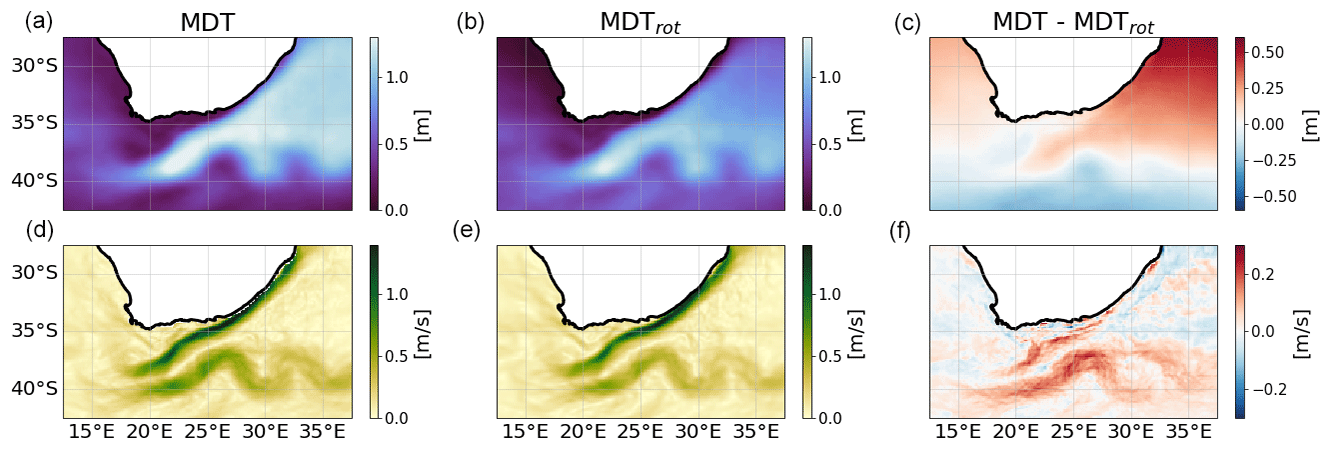
Figure 1 (a–c) Raw MDT field (a), its rotational part (b) and the difference between the two (c). (d–f) Absolute geostrophic velocity computed from the associated top fields using Eq. (4).

2.3 Data assimilation

The SLA observations (denoted as SLA^obs) are assimilated into the QG model with the back-and-forth nudging (BFN, Auroux and Blum, 2008) technique. This technique is based on the nudging strategy, which consists of gently pulling the model trajectory towards the observations. Mathematically, an extra term proportional to the difference between the model SLA and the observations is added in Eq. (8):

$$\begin{array}{}\text{(9)}& {\displaystyle \frac{\partial q^{\prime }}{\partial t}}+\stackrel{\mathrm{‾}}{{\mathit{u}}_{\mathrm{g}}}\cdot \mathrm{\nabla }{q}^{\prime }+{\mathit{u}}_{\mathrm{g}}^{\prime }\cdot \mathrm{\nabla }\stackrel{\mathrm{‾}}{q}+{\mathit{u}}_{\mathrm{g}}^{\prime }\cdot \mathrm{\nabla }{q}^{\prime }=K({\mathrm{SLA}}^{\mathrm{obs}}-\mathrm{SLA}),\end{array}$$

where K is the tunable nudging coefficient. Its value determines the balance between the weights given to the observations and the QG dynamics. As explained in Le Guillou et al. (2021a), K varies in time and space to allow a smooth nudging of the model towards the observations. Mathematically, the nudging coefficient at time t and at the model grid point x is computed by the following equation:

$$\begin{array}{}\text{(10)}& K(x,t)=K_{\mathrm{0}}\sum _{i=\mathrm{1}}^{N_{\mathrm{obs}}}{e}^{-{\left(\frac{\left|\right|x-x_i\left|\right|}{D}\right)}^{\mathrm{2}}}{e}^{-{\left(\frac{t-t_i}{\mathit{\tau }}\right)}^{\mathrm{2}}},\end{array}$$

where K₀ is the nominal value of the nudging coefficient, N_obs is the number of observations, and (x_i,t_i) are the space–time coordinates of the ith observation. D and τ are the spatial and temporal scales at which the model is nudged towards the observations, impacting directly the scales of the reconstructed structures.

The BFN algorithm calls iteratively the forward nudging, defined as a forward-in-time propagation of Eq. (9) with K>0, and the backward nudging, defined as a backward-in-time propagation of Eq. (9) with K<0, within a fixed temporal window T. The temporal window T has to be chosen considering the observation sampling, the decorrelation time of the QG model and the computational complexity. At the beginning of each temporal loop, the SLA variable is initialized with the value estimated from the previous loop. In a few iterations (less than 20), the BFN converges towards a trajectory that fits both the observations and the model dynamics. For more details on the BFN-QG technique, the reader is referred to Auroux and Blum (2008), Amraoui et al. (2023) and Le Guillou et al. (2021a).

3 Experimental setup

3.1 Study area and input data

We assess the BFN-QG performances in a part of the Agulhas Current (25–45^∘ S, 10–40^∘ E) from 1 January 2010 to 31 December 2019. The Agulhas Current is the major western boundary current of the Southern Hemisphere, transporting large volumes of warm and saline water from the Indian Ocean to the Atlantic Ocean, greatly impacting climate (Bryden et al., 2005) and vessel trajectories (Le Goff et al., 2021).

As input data of the BFN-QG, we use the along-track L3 filtered SLA products from Jason-3, Sentinel-3A, Sentinel-3B, HaiYang-2, CryoSat-2 and SARAL/AltiKa. These SLAs have been distributed by the CMEMS (http://marine.copernicus.eu/, last access: October 2023) after the reprocessing of 25 years of altimetric data (Taburet et al., 2019). For our analysis, we use the spatially filtered data, whose cutoff has been set to 65 km, corresponding to altimeters' effective resolutions (Pujol et al., 2016).

3.2 Mean geostrophic current

The mean state of the ocean surface needed to advect the QG potential vorticity anomaly q^′ through Eq. (8) is extracted from the CNES-CLS18 mean dynamic products (Mulet et al., 2021). In this product, the topography (MDT) and velocity (MDV for mean dynamical velocity vector) are estimated with a multivariate objective analysis of a combination of altimeter and space gravity data and in situ measurements. A central step of the analysis lies in the filtering of the ageostrophic component of the in situ velocity measurements.

In Eqs. (8) and (9), both $\stackrel{\mathrm{‾}}{{\mathit{u}}_{\mathrm{g}}}$ and $\stackrel{\mathrm{‾}}{q}$ have to be prescribed. For reasons not investigated during this work, the MDV product is not divergence free. Because $\stackrel{\mathrm{‾}}{{\mathit{u}}_{\mathrm{g}}}$ must be divergence free by construction (after Eq. 4), we prescribe it with the divergence-free part of the MDV, called MDV_rot (the subscript indicates that MDV_rot contains the rotational part of the MDV). The field MDV_rot is computed with the geostrophic Eq. (4) from a mean dynamic topography called MDT_rot, obtained after solving the following elliptic equation:

$$\begin{array}{}\text{(11)}& \mathrm{\Delta }\left({\mathrm{MDT}}_{\mathrm{rot}}\right)={\displaystyle \frac{g}{f}}\mathbf{\nabla }\times \mathit{M}\mathit{D}\mathit{V}.\end{array}$$

The rotational operator on the right rules out the divergent part of the MDV. For consistency, $\stackrel{\mathrm{‾}}{q}$ is diagnosed from Eq. (1) and MDT_rot. Figure 1 indicates the significance of this procedure: the original MDT and MDV differ from their divergence-free counterparts by the orders of magnitude of the fields.

At the end of the mapping processing, we add the full MDV to the estimated velocity anomalies.

3.3 Performance assessment strategies

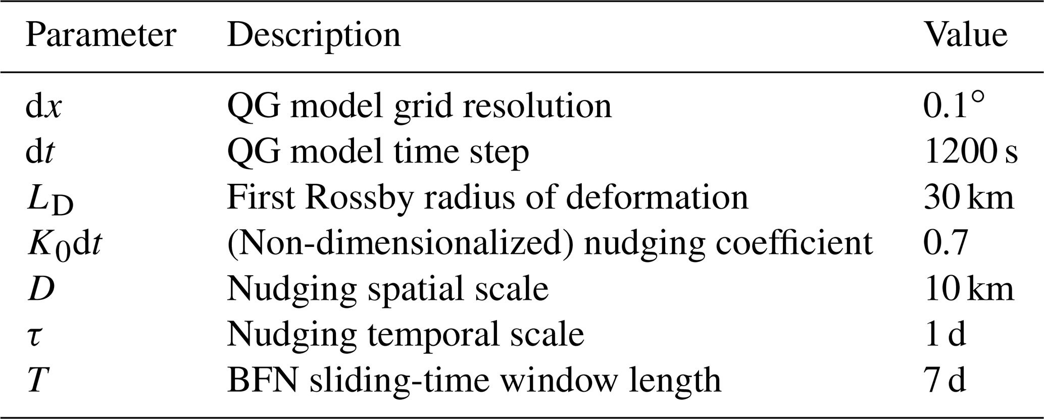
We compare the performances of the BFN-QG system and the DUACS DT2018 system (Taburet et al., 2019). We use the global daily product provided by CMEMS on a 0.25^∘ latitude × 0.25^∘ longitude grid. The BFN-QG is run on a 0.1^∘ latitude × 0.1^∘ longitude grid, and the output maps are saved every 3 h. The parameters of the BFN-QG (defined in the previous sections) have been prescribed after a sensitivity experiment and are listed in Table 1.

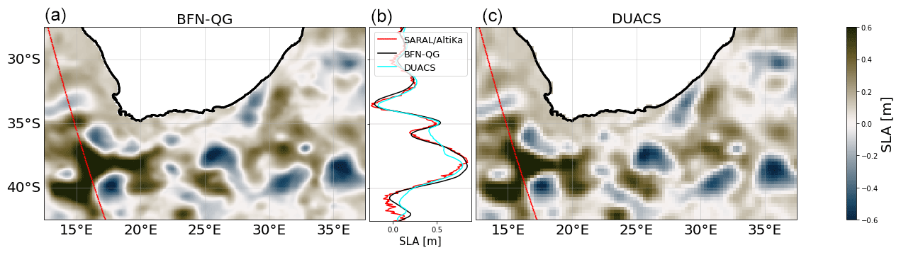
Figure 2 SLA mapped by the BFN-QG (a) and DUACS (c) systems on 15 October 2019. The fields are plotted with native spatial resolution (0.25^∘ for the DUACS product, 0.1^∘ for the BFN-QG product). The red lines represent the track of the independent SARAL/AltiKa altimeter at this date. Panel (b) compares the independent 1D SLA profile with the estimated SLAs interpolated on the track location.

Table 1 BFN-QG parameters.

The comparison focuses on SLA (hereafter called SLA mapping; see Sect. 4) and geostrophic currents (hereafter called velocity mapping; see Sect. 5). For assessing the SLA-mapping capability, we exclude SARAL/AltiKa from the altimetric observation network to use it as independent data, and we focus only on the year 2019. For assessing the velocity-mapping capability, all the available altimetric observation networks are used, and the validation is performed with independent drifter and SST data over the entire time period (10 years).

4 SLA-mapping performances

The SLA-mapping performances are assessed by comparing the mapped products with the independent altimetric data, following the same method as in Ballarotta et al. (2020). The estimated gridded maps noted ($\widehat{\mathrm{SLA}}$) are interpolated on the locations of the independent measurements (SLA^ind) to compute the differences: $\mathrm{\Delta }\mathrm{SLA}=\widehat{\mathrm{SLA}}-{\mathrm{SLA}}^{\mathrm{ind}}$. Figure 2 shows maps from BFN-QG and DUACS for 1 single day with a SARAL/AltiKa altimeter track superimposed. SARAL/AltiKa SLA observations and SLA interpolated from both maps onto the satellite track are shown in the middle panel. In the case presented here, the BFN-QG result fits the independent observations (SLA^ind) better than the DUACS product.

A first quantitative comparison between BFN-QG and DUACS over the whole 2019 year is performed with root mean square errors (RMSEs). As the independent data are sparse, the differences ($\mathrm{\Delta }\mathrm{SLA}=\widehat{\mathrm{SLA}}-{\mathrm{SLA}}^{\mathrm{ind}}$) are aggregated in 1^∘ latitude × 1^∘ longitude boxes to give the spatial distribution of the errors. For each box, the RMSE is computed as follows:

$$\begin{array}{}\text{(12)}& \mathrm{RMSE}={\displaystyle \frac{\mathrm{1}}{N}}\sum _{i=\mathrm{1}}^N[\mathrm{\Delta }{\mathrm{SLA}}_i{]}^{\mathrm{2}},\end{array}$$

where N is the number of independent observations in a specific grid box. Before computing the RMSE, we can apply a spatial filtering to ΔSLA to isolate frequency bands of interest. In the present case, we filter out scales larger than 300 km in order to focus on the estimation of mesoscale structures (right panel of Fig. 3). The comparison of the performances of the BFN-QG versus DUACS is then given by the gain $/$ loss ratio R:

$$\begin{array}{}\text{(13)}& R={\displaystyle \frac{{\mathrm{RMSE}}_{\text{BFN-QG}}-{\mathrm{RMSE}}_{\mathrm{DUACS}}}{{\mathrm{RMSE}}_{\mathrm{DUACS}}}}.\end{array}$$

A second quantitative evaluation of the scale-wise mapping performances is carried out with a spectral analysis. As before with RMSEs, the analysis is applied to the reconstructed SLAs interpolated on the independent tracks. Each independent satellite track in the study area is split into 800 km segments overlapping every 200 km. The data along the segments are then detrended, and a Hanning window is applied. We use the Welch (Welch, 1967) method to compute the power spectral density (PSD) distribution for each segment. We average the PSDs for all segments to get a statistically robust estimation of the energy distribution among spatial scales. We also compute the wavelength-dependent PSD score, SPSD, defined as follows:

$$\begin{array}{}\text{(14)}& \mathrm{SPSD}=\mathrm{1}-{\displaystyle \frac{\mathrm{PSD}\left(\mathrm{\Delta }\mathrm{SLA}\right)}{\mathrm{PSD}\left({\mathrm{SLA}}^{\mathrm{ind}}\right)}}.\end{array}$$

SPSD is equal to 1 for a perfect reconstruction and 0 when the error is as energetic as the observed oceanic signal. The effective resolution of the maps is defined as the spatial scale for which the spectral score is equal to 0.5.

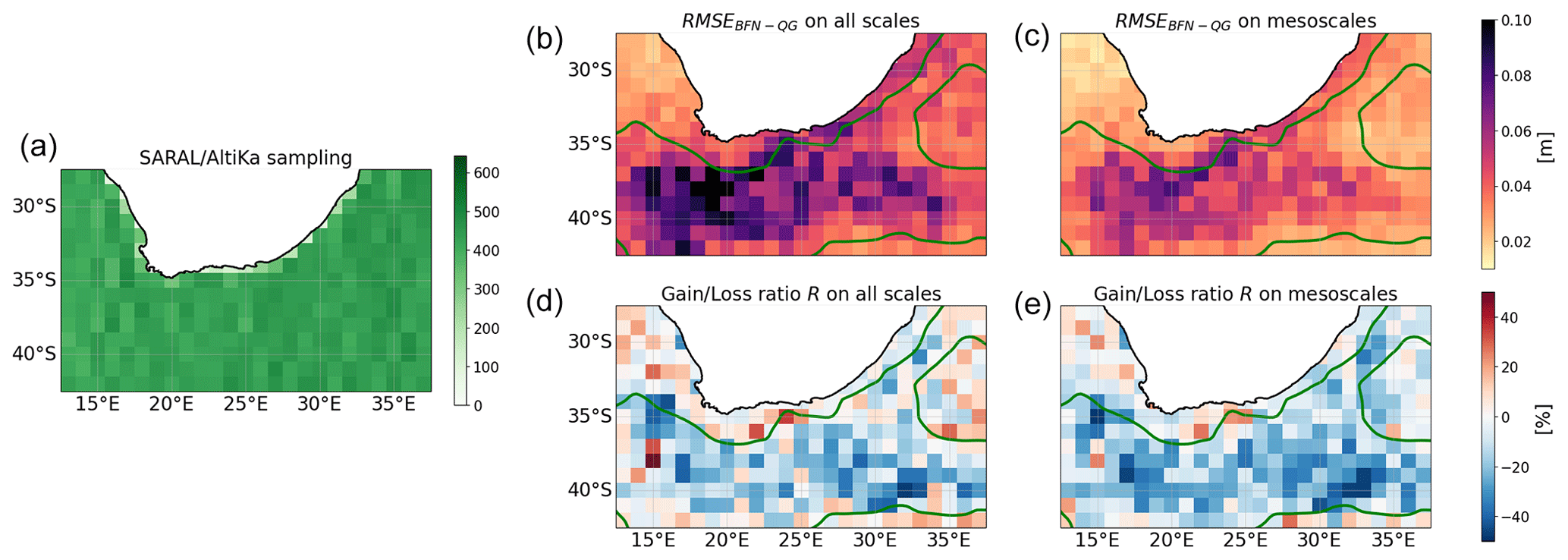
Figure 3 Geographical statistics of the SLA-mapping performances for the year 2019. (a) Number of independent SARAL/AltiKa altimeter data items available. (b–e) RMSE of the BFN-QG (b, c) and the gain $/$ loss ratio R with respect to DUACS (d, e) for all spatial scales (b, d) and mesoscales (c, e). Negative values (blue) indicate better performances for the BFN-QG method compared to DUACS. The green contour is the 200 cm² SSH variance contour.

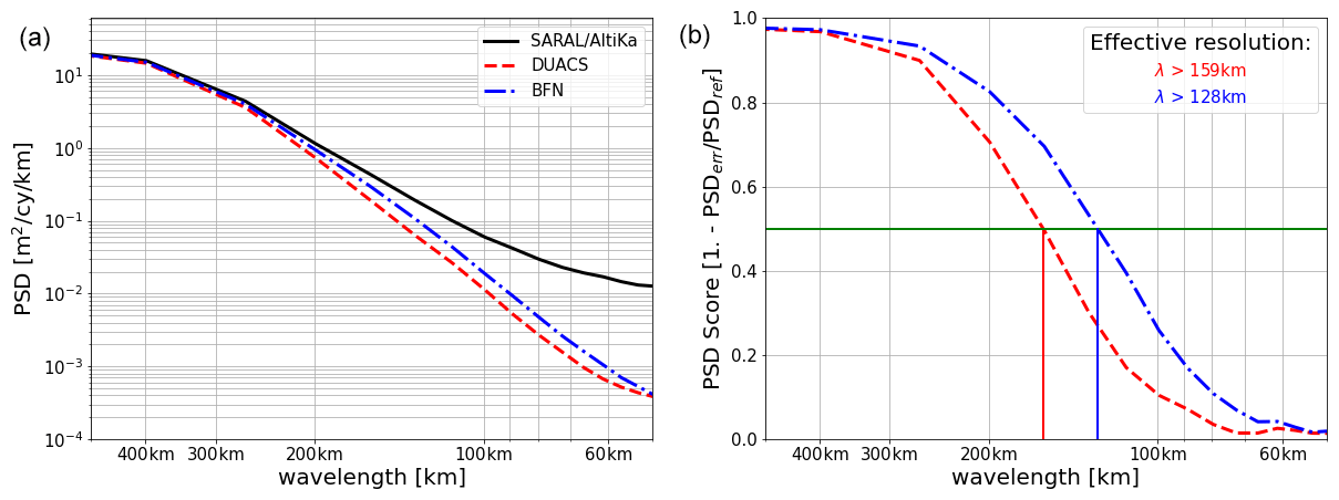
Figure 4 Spectral diagnostics: PSD (a) and associated scores (b) of the mapped products. The intersections between the horizontal green line (corresponding to a PSD score of 0.5) and the curves define the effective resolutions of the products.

The results of the quantitative evaluations are reported in Figs. 3 and 4. Figure 3 shows the number of observations per box, the spatial distribution of RMSE_BFN-QG and R for all scales and for the mesoscales. Figure 4 presents the PSDs and the PSD scores.

The BFN-QG considerably improves the mapping of energetic mesoscale structures compared to DUACS. In terms of RMSEs, the improvement (i.e., density and intensity of blue pixels in Fig. 3, right) is higher for the mesoscales (defined as scales below 300 km) than for all scales. This is corroborated by the spectral analysis, which shows that the BFN-QG maps are in better agreement (both in amplitude and phase) with the independent data, especially for scales below 300 km. The effective resolution of the maps is improved by a factor of 20 compared to DUACS (Fig. 4 right). The performances of the BFN-QG are reduced for larger spatial scales and in low-variability regions. For scales higher than 300 km, DUACS outperforms the BFN-QG on average by a factor of 1.3 in terms of spectral score. For all scales, the improvement brought about by the BFN-QG is reduced in low-variability regions (delimited by the green contours in Fig. 3). These weak performances of the BFN-QG in reconstructing the large-scale structures may be due to the way we compute the nudging coefficient K (through Eq. 10), whose spatial and temporal scales (see Table 1) have been tuned to enhance the mapping of short-scale dynamics.

5 Velocity-mapping performances

5.1 Validation with drifter data

In this section, the velocity-mapping performances are assessed using independent drifter data at hourly resolution, selected from Elipot et al. (2016). The ageostrophic component of the observed velocities has not been removed in these reference data as we assume that it should affect the performance of the DUACS and BFN-QG methods in the same way. Snapshots of the norm of geostrophic velocities from the BFN-QG and DUACS systems are shown in Fig. 5. At first sight, the currents estimated by the BFN-QG exhibit finer-scale structures (filaments and small vortices) than the ones derived from DUACS. Figure 5 is further discussed later.

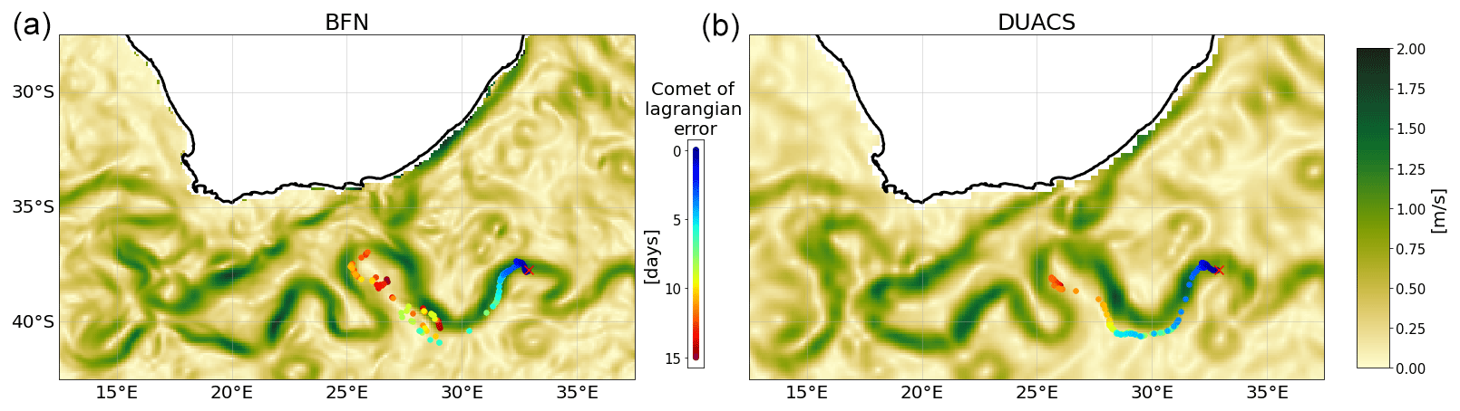
Figure 5 Geostrophic currents mapped by the BFN-QG (a) and DUACS (b) systems on the 2 November 2019. The red cross represents the location of one drifter at this date. The colored dots represent the expected drifter positions as predicted from the true past positions with the mapped currents. The dot color indicates the prediction lead time. For example, the yellow dots are predictions initialized 9 d in the past. Their distances to the red cross indicate the prediction errors.

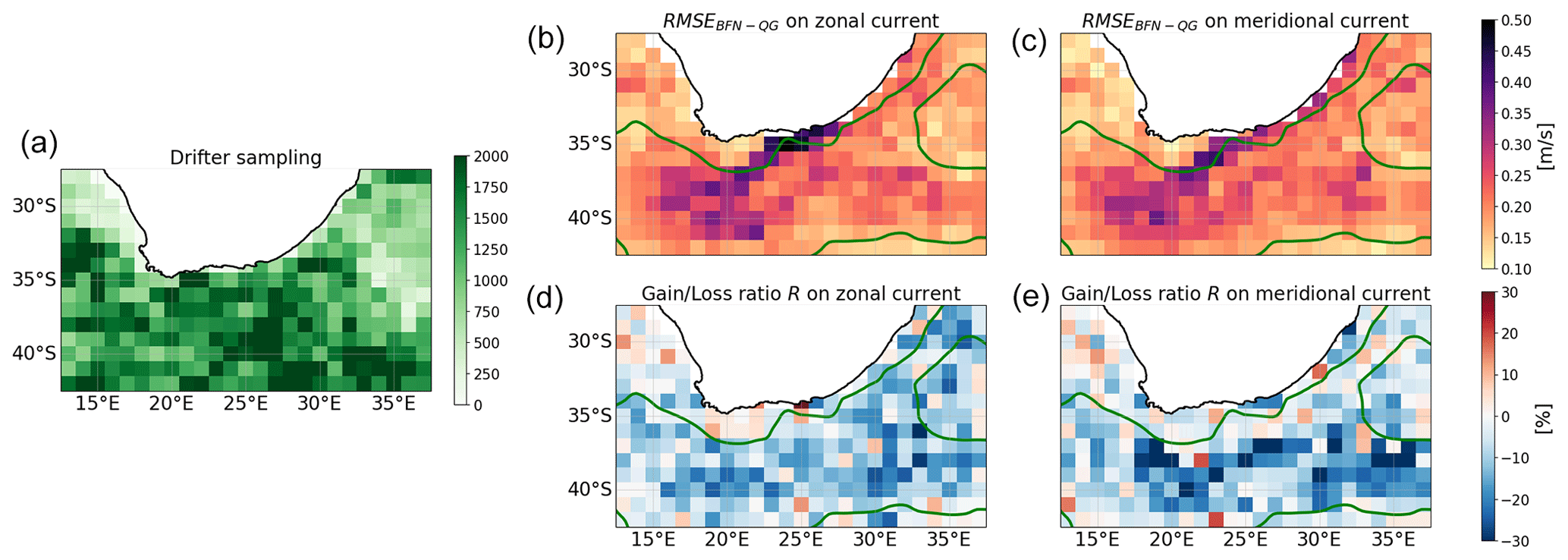
Figure 6 Geographical statistics of the velocity-mapping performances for the 10 years studied (from 2010 to 2019). (a) Independent drifter sampling. (b–e) RMSE of the BFN-QG (b, c) and the gain $/$ loss ratio R with respect to DUACS (d, e) for the zonal (b, d) and meridional (c, e) currents. Negative values (blue) indicate better performances for the BFN-QG method compared to DUACS. The green contour is the 200 cm² SSH variance contour.

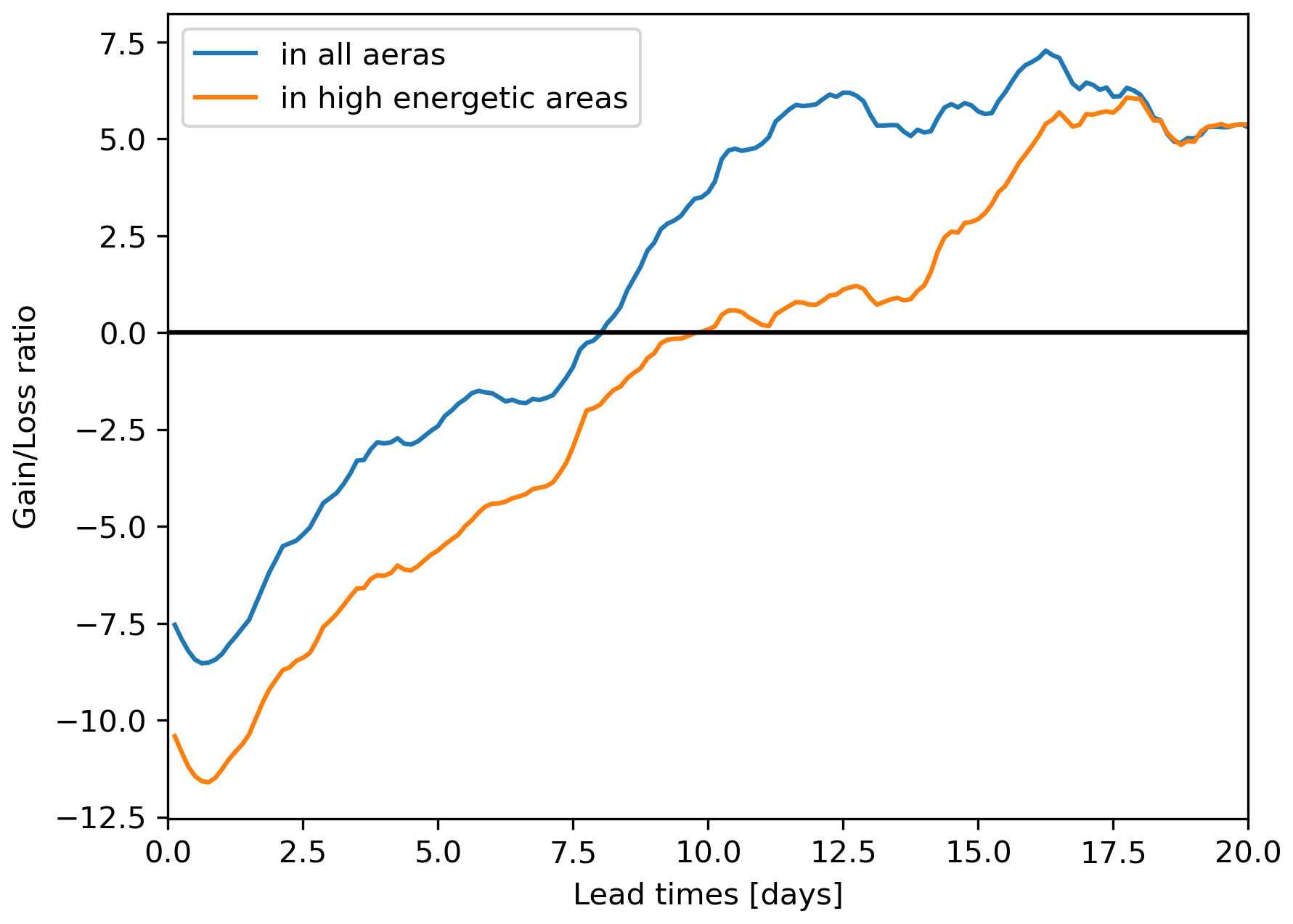
Figure 7 Gain $/$ loss ratio for the predictability of the mapped surface geostrophic current for estimating Lagrangian transport as a function of the prediction lead times. Negative values indicate better performances for the BFN-QG method compared to DUACS. In blue, all the drifter data available in the experimental time period are considered. In orange, only the drifters located in the highly energetic regions are considered.

A performance diagnostic of an Eulerian nature is performed by comparing the estimated currents with the velocities measured by the drifters at each drifter location (in space and time). We use the same methodology as for the SLA-mapping performances: the mapped velocities (meridional and zonal components) are interpolated on the drifters' locations, and the errors with the drifters' velocities are aggregated in 1^∘ latitude × 1^∘ longitude boxes. The RMSE and the gain $/$ loss ratio R (Eq. 13) are then computed in each box. The results are reported in Fig. 6. The geographical distribution of the gain $/$ loss ratio R shows a net improvement in the estimation of both zonal and meridional currents. This improvement is more pronounced for the meridional component, which is often harder to estimate from altimetry compared to the zonal component due to the nearly meridional orientation of the altimetry tracks. Like the SLA mapping, more improvements (as before, this is a relative comparison in %) occur in high-variability regions, as shown by the intensification of blue pixels in the inner domain delimited by the green contour in Fig. 6. Besides, the relative performances of the BFN-QG in low-variability regions are better for the velocity mapping than for the SLA mapping. This is probably due to the fact that the low-variability dynamics occur at large scales, which have very little impact on geostrophic currents.

The second performance diagnostic is Lagrangian: simulated drifter trajectories are compared with the real ones. For one drifter at one time, we compute the distances between the real drifter location and the locations predicted with the evaluated velocity fields. The predictions are initialized with the real drifter locations at earlier times ranging from 0 to 20 d, every 3 h. As an example, Fig. 5 displays the results for one drifter and one time. The BFN-QG-derived geostrophic currents improve the prediction of short-term Lagrangian transport compared to the DUACS-derived geostrophic currents: the blue dots, representing Lagrangian predictions with lead time up to 5 d, are much closer to the real location of the drifter for the BFN-QG system than for DUACS. But the red dots, representing Lagrangian predictions higher than 10 d, are as far as the ones predicted by DUACS. To investigate the lead time dependency of the relative performances of BFN-QG and DUACS in this Lagrangian diagnostic, the gain $/$ loss ratios are plotted as a function of lead time in Fig. 7. The BFN-QG improves the Lagrangian prediction by more than 7 % for 1–3 d lead times compared to DUACS, with an enhanced improvement for drifters located in high-variability regions. The gain $/$ loss ratio becomes positive (which means better performances for DUACS compared to the BFN-QG) for lead times higher than 10 d. The standard deviation of the Lagrangian errors (not shown) is higher for the BFN-QG than for DUACS, and this is accentuated for long lead times. This is qualitatively visible in Fig. 5 where the distances between the expected locations and the real location of the drifter increase almost linearly with the lead times for DUACS, while they are much more scattered for the BFN-QG (especially for lead times higher than 10 d). This can be explained by the higher spatial resolution of the BFN-QG fields.

5.2 Validation with SST data

This section compares the positions of fronts and eddies diagnosed from our reconstructions with those diagnosed from high-resolution SST observations. To do so, we use the Fronts Derived from Remote Sensing SST Observations by SEVIRI (Spinning Enhanced Visible and InfraRed Imager) over the Agulhas Region dataset created within the ESA World Ocean Circulation (WOC) project (https://doi.org/10.12770/6c776c43-425b-4d29-9934-0822696f15d8) as ground truth. For each point ($P_i=\left[\begin{array}{c}{\mathrm{lon}}_i\\ {\mathrm{lat}}_i\end{array}\right]$) of the detected frontal structures, we compute the flow crossing the fronts using either BFN-QG or DUACS geostrophic currents:

$$\begin{array}{}\text{(15)}& \mathrm{Flow}\left[P_i\right]=\left|{\displaystyle \frac{\mathit{v}\left[P_i\right]\cdot {\mathit{\delta }}_i}{\Vert \mathit{v}\left[P_i\right]\Vert \Vert {\mathit{\delta }}_i\Vert }}\right|=\left|\cos \widehat{\left(\mathit{v}\right[P_i],{\mathit{\delta }}_i)}\right|,\end{array}$$

where v[P_i] is the velocity vector at point P_i, ${\mathit{\delta }}_i=\left[\begin{array}{c}{\mathrm{lat}}_{i+\mathrm{1}}-{\mathrm{lat}}_{i-\mathrm{1}}\\ -({\mathrm{lon}}_{i+\mathrm{1}}-{\mathrm{lon}}_{i-\mathrm{1}})\cos \left({\mathrm{lat}}_i\right)\end{array}\right]$ is the normal vector of the front at point P_i, and $\widehat{\left(\mathit{v}\right[P_i],{\mathit{\delta }}_i)}$ is the angle between v[P_i] and δ_i. The values of the flow range from 0 to 1. Assuming that SST fronts and currents are aligned, the lower the flow, the more consistent the current estimation is with the SST. For this analysis to be valid, the currents have to be in geostrophic balance, and the advection of frontal structures must be negligible.

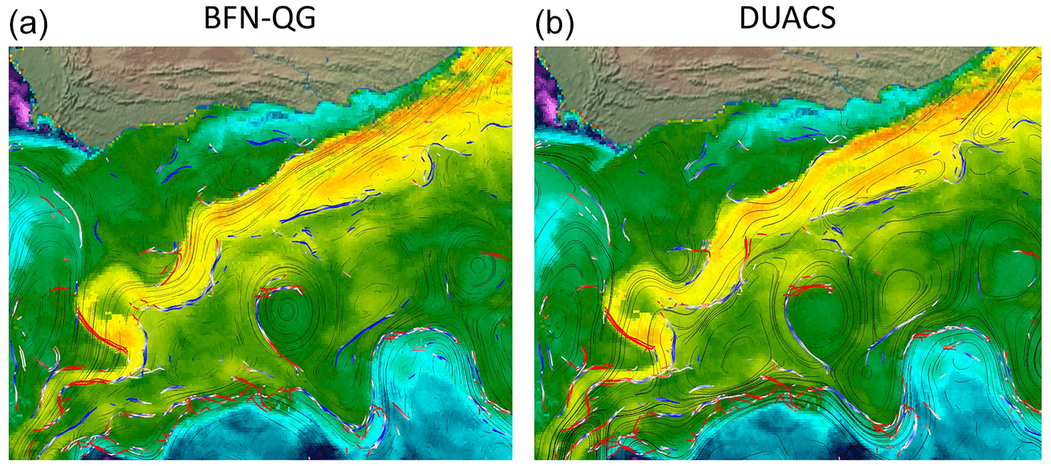
Figure 8 Snapshots showing the geostrophic current streamlines computed from the BFN (a) and DUACS (b) on top of the SEVIRI SST for which the detected frontal structures are depicted by the colored lines (in blue for small values of the crossing flow, red for high values). These snapshots are taken from the Ocean Virtual Laboratory web portal (https://odl.bzh/rvYm4Bv0, last access: October 2023).

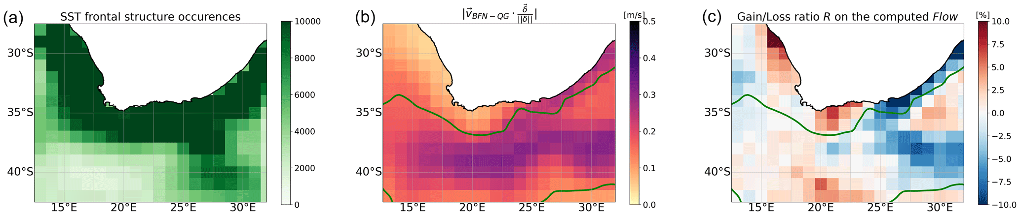
Figure 9 Geographical distribution of the frontal structure occurrences during the 10 years of comparison (a), the averaged BFN-QG currents crossing the SST fronts (b) and the gain $/$ loss ratio R with respect to DUACS (c). The green contour is the 200 cm² SSH variance contour.

The Agulhas Current area is an excellent natural laboratory for this kind of analysis, with a strong geostrophic current, strong SST gradients and relatively weak advection of the frontal structures. However, the presence of Natal pulses in the nearshore side of the Agulhas Current core (Krug and Penven, 2011) and complicated dynamics occurring in the retroflection area (Zhu et al., 2021) may advect significantly the frontal structures and thus limit this analysis. An illustration of the comparison of fronts and velocity is shown in Fig. 8. The direction of the streamlines derived from the BFN-QG (left) and DUACS (right) can be compared. One can visually see that the sharp turn of the Agulhas Current is better represented in the BFN-QG than in DUACS.

Figure 9 shows statistics of the crossing flow computed from the geostrophic currents derived both from the BFN-QG and DUACS techniques within the 10-year study period. As for the previous diagnostics, the statistics are aggregated in 1^∘ latitude × 1^∘ longitude boxes. The left panel of Fig. 9 indicates that all pixels of the region are covered by several thousands of SST front occurrences, hence providing reliable statistics. The number of occurrences depends on the probability of detecting frontal structures and the cloud cover.

The statistics show mixed performances of the BFN-QG compared to DUACS, with stronger geographical patterns than with the previous diagnostics (see Sects. 4 and 5). In particular, the meanders of the Agulhas Current are well captured by the BFN-QG, and the improvement in the main current is significant. On the other hand, in some regions, DUACS significantly outperforms the BFN-QG. We note that these regions are mostly characterized by weak crossing currents, as shown in the middle panel of Fig. 9. One example is the Agulhas Bank, i.e., the coastal region south of Africa characterized by very shallow waters. In this region, the weak performances of the BFN-QG are probably due to the non-representation of the bathymetry in the QG model (whose variations strongly affect the value of the Rossby radius of deformation L_D, which modulates the potential vorticity field, through Eq. 1). This shows that the method needs to be improved to better perform in coastal areas. Finally, Fig. 9 also depicts weak performances of the BFN-QG (compared to DUACS) in the southwestern part of the study domain, which is in contradiction with the other diagnostics. This can be due to non-reliable statistics because of the weaker density of observations and/or too-strong advection of the fronts by the currents that limits the validity of the analysis.

6 Discussion and conclusions

In this study, we follow on the analysis presented in Le Guillou et al. (2021a) for assessing the performances of the BFN-QG to map altimetry data. The BFN-QG is a non-common data assimilation technique that can be used to dynamically map altimetry data. This dynamical mapping technique shares similarities with the DOI experimental mapping technique (Ubelmann et al., 2016; Ballarotta et al., 2020). The major advantage of the BFN-QG technique over the DOI technique is the very limited number of parameters to tune and its relatively low numerical cost. Le Guillou et al. (2021a) considered simulated observations for testing the impact of the SWOT mission on the mapping capabilities. Here, the BFN-QG is tested to map real along-track altimetry data in a region covering the highly energetic Agulhas Current. The performances are assessed by comparing the mapped products, from BFN-QG and from the operational reference DUACS, with independent datasets. We have carried out diagnostics on mapped SLA (using independent altimetric data) and mapped velocity (using independent drifters and high-resolution SST data).

The BFN-QG improves the mapping of short, energetic mesoscale structures in both space and time in comparison with the DUACS system. The BFN-QG is able to reconstruct finer coherent structures that are in phase with observations from independent datasets. The spatial effective resolution is improved by a factor of 20 compared to DUACS. The prediction of Lagrangian transport by the BFN-QG-derived geostrophic currents is improved for lead times of up to 10 d in comparison with the DUACS-derived geostrophic currents

The performances of the BFN-QG are not uniform for all temporal and spatial scales. The method fails to improve the mapping of large mesoscale structures (>300 km) in comparison with DUACS. This is corroborated by the poor performances of the BFN-QG-derived currents in estimating the Lagrangian transport for lead times larger than 10 d. Future works should investigate the implementation of a multi-scale nudging whose parameters vary with the spatial and temporal scales of the dynamics (Stauffer and Seaman, 1994). This would prevent departure from large-scale circulation while maintaining the accuracy of the mapping of small scales.

Another issue with the BFN-QG lies in its poor performances in mapping low-energy dynamics. This disagrees with the previous study of Le Guillou et al. (2021a), which showed similar performances in low- and high-variability regions. One difference here is that the study region exhibits strong variations in bathymetry, limiting the validity of the quasi-geostrophic assumption. Another difference is that the observations contain measurement noise that may become important in low-variability regions given the fact that the OI allows a better representation of measurement noise (through the observation covariance matrix) than the BFN-QG does (having only one tunable scalar factor, K). Finally, the observations can contain the signature of non-geostrophic dynamics, such as internal tides, which can be strong in low-variability regions (Qiu et al., 2018). A natural perspective would be to test the method presented in Le Guillou et al. (2021b) to jointly map internal tides and balanced motions from real altimetric observations.

With the advent of swath altimetry through the just-launched SWOT mission, future works should investigate the estimation of the geostrophic dynamics of baroclinic modes higher than the first one. In this study, we have assimilated the SSH observations in a simple 1.5-layer QG model (which simulates the dynamics of the first baroclinic mode) to ensure its good controllability with sparse along-track altimetric data. Indeed, we deeply believe that the performances of the assimilation procedure rely on the balance between the density of observations and the complexity of the dynamical model. The very high density of SSH observations from the SWOT mission might enable the use of multiple-layer QG models to improve the reconstruction of the geostrophic dynamics.

Finally, this study's approach might be further strengthened by exploiting the synergies between altimetry and other space-borne data to improve the reconstruction of small-scale ocean surface dynamics. First, as performed in this paper for validation purposes, altimetry can be combined with observations of surface tracers such as SST and chlorophyll concentration to estimate the ocean surface currents. Similarly to potential vorticity, which is advected by geostrophic currents, tracers are advected by total (geostrophic + ageostrophic) currents (Rio and Santoleri, 2018; Ciani et al., 2021). To extend our present data assimilation strategy, the tracer observations could be assimilated in simple tracer advection–diffusion models. Second, data acquired by the Sentinel-1 Interferometric Wide mode can be processed to extract (radial) ocean surface velocities (Moiseev et al., 2020) that might complement the altimetric sampling, especially in coastal areas where this mode is active. Third, preparatory works should investigate the best strategies to integrate data from future Doppler satellite missions, like the NASA/CNES ODYSEA (Ocean DYnamics and Surface Exchange with the Atmosphere) mission (Villas Bôas et al., 2019; Rodríguez et al., 2019), to reconstruct the ocean surface dynamics at small scales.