Seasonal cycle of sea surface temperature in the tropical Angolan Upwelling System

The Angolan shelf system represents a highly productive ecosystem. Throughout the year the sea surface is cooler near the coast than further offshore. The lowest sea surface temperature (SST), strongest cross-shore temperature gradient, and maximum productivity occur in austral winter when seasonally prevailing upwelling-favourable winds are weakest. Here, we investigate the seasonal mixed layer heat budget to identify atmospheric and oceanic causes for heat content variability. By using different satellite and in situ data, we derive monthly estimates of surface heat fluxes, mean horizontal advection, and local heat content change. We calculate the heat budgets for the near-coastal and offshore regions separately to explore processes that lead to the observed SST differences. The results show that the net surface heat flux warms the coastal ocean stronger than further offshore, thus acting to damp spatial SST differences. Mean horizontal heat advection is dominated by meridional advection of warm water along the Angolan coast. However, its contribution to the heat budget is small. Ocean turbulence data suggest that the heat flux, due to turbulent mixing across the base of the mixed layer, is an important cooling term. This turbulent cooling, being strongest in shallow shelf regions, is capable of explaining the observed negative cross-shore temperature gradient. The residuum of the mixed layer heat budget and uncertainties of budget terms are discussed.

1 Introduction

The coastal waters off Angola host a highly productive ecosystem of great socio-economic importance for local communities: the tropical Angolan Upwelling System (tAUS) (Sowman and Cardoso, 2010; FAO, 2018). The Congo River outflow at 6^∘ S forms the northern boundary of the tAUS. To the south the Angola–Benguela Frontal Zone located between 15 and 18^∘ S separates the warm surface waters of the tAUS from colder water further south (Fig. 1a). The tAUS is characterized by lower sea surface temperatures (SSTs) near the coast compared to further offshore throughout the year (Fig. 1a). In austral winter we find the lowest SSTs, the strongest negative cross-shore SST gradient, and the maximum in primary productivity in the tAUS (Fig. 2, Tchipalanga et al., 2018; Zeng et al., 2021, Awo et al., 2022). Thus, understanding the drivers of heat content changes in the upper ocean in the tAUS might be important for the understanding of productivity as well. Additionally, it is also of larger-scale importance due to the remote impact of the southeastern tropical Atlantic on tropical climate (Xu et al., 2014).

Figure 1 (a) Mean sea surface temperature (SST) (colours) and schematic circulation in the southeastern tropical Atlantic. Solid arrows indicate pathways of surface currents and dashed arrows of subsurface currents. Currents displayed here are the Equatorial Undercurrent (EUC), the Gabon Congo Undercurrent (GCUC), the South Equatorial Undercurrent (SEUC), the South Equatorial Countercurrent (SECC), the Angola Current (AC), and the Benguela Coastal Current (BCC). Additionally, the position of the Angola–Benguela Frontal Zone (ABFZ) is marked. (b) Topography (colours) and mean wind field (arrows) off the coast of southwestern Africa. Black lines mark the 75 and 175 m isobath. Red boxes show the extent of the coastal and offshore boxes. The red star marks the position of the PIRATA-SEE mooring. The black line shows the 11^∘ S section.

The circulation in the tAUS is dominated by the Angola Current (Fig. 1a) whose core is located at around 50 m depth. The Angola Current transports warm water poleward along the Angolan continental slope and shelf. The transport is weak (∼ 0.32 SV) and subject to variability on different timescales (Kopte et al., 2017). Past studies showed that the variability is connected to equatorial dynamics via the propagation of equatorial and coastal trapped waves (CTWs) as well as to local forcings (Bachèlery et al., 2016; Kopte et al., 2017; Illig et al., 2018). The Angola Current is fed via the Equatorial Undercurrent, the South Equatorial Undercurrent, and the South Equatorial Countercurrent with South Atlantic Central Water (Kopte et al., 2017; Tchipalanga et al., 2018; Siegfried et al., 2019). In the Angola–Benguela Frontal Zone, the poleward Angola Current meets the northward Benguela Coastal Current (Shannon et al., 1987; Siegfried et al., 2019; Fig. 1a).

The surface waters in the tAUS are characterized by warm tropical conditions (Tchipalanga et al., 2018; Awo et al., 2022; Fig. 1a). In austral winter the lowest SSTs are observed (Fig. 2). The SST at the coast can then drop below 21 ^∘C. Highest temperatures are found in austral autumn when coastal SSTs reach 28 ^∘C (Fig. 2, Awo et al., 2022). In contrast to other eastern boundary upwelling systems, the changes in surface temperatures, cross-shelf temperature gradient, and productivity in the tAUS cannot be explained by local wind-driven upwelling (Ostrowski et al., 2009). On average, the winds in tAUS are southwesterly and substantially weaker than in the Benguela upwelling system further south (Fig. 1b). They have a weak seasonal cycle with a minimum in upwelling-favourable winds during the upwelling season in austral winter (Ostrowski et al., 2009; Zeng et al., 2021).

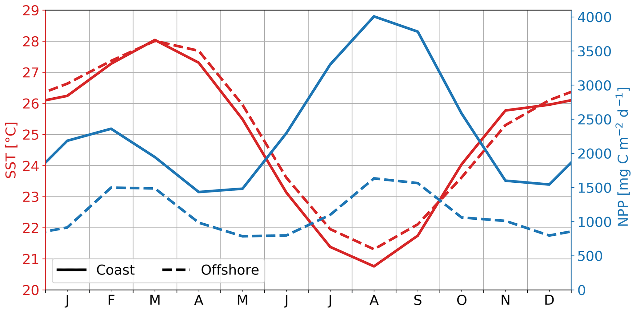
Figure 2 Seasonal cycle of SST (red) and net primary production (blue) averaged over the coastal box (solid lines) and offshore box (dashed lines) shown in Fig. 1b.

Changes in upper-ocean heat content in the tAUS can be affected by the passage of remotely forced CTWs. The CTWs have a signal in sea level anomaly (SLA). Analysing SLA data in the tAUS reveals the passage of four CTWs per year (Rouault, 2012). In March a downwelling CTW propagates along the Angolan coast followed by an upwelling CTW in June–July. In October a second downwelling CTW arrives at the Angolan coast followed by a weak upwelling wave in December–January (Tchipalanga et al., 2018). Thus, the upwelling season coincides with the presence of an upwelling CTW at the Angolan coast. However, the vertical movement of the thermocline alone is unable to explain the near-coastal cooling and the upward nutrient supply during austral winter. In this context, the role of mixing induced by internal tides has been discussed (Ostrowski et al., 2009; Tchipalanga et al., 2018; Zeng et al., 2021). Zeng et al. (2021) showed in a recent model study that seasonal variations in the spatially averaged generation, onshore flux, and dissipation of internal tide energy are weak. Due to the seasonal variation in stratification, however, turbulent mixing driven by internal tides is more effective in reducing the SST during the upwelling season.

The sea surface salinity (SSS) undergoes a distinct seasonal cycle in the tAUS (Awo et al., 2022). In October–November and in February–March fresh water intrudes into the northern part of the tAUS (Kopte et al., 2017; Lübbecke et al., 2019; Awo et al., 2022). A recent model study (Awo et al., 2022) suggests that the freshening is controlled by meridional advection via the Angola Current, with the Congo River as an important freshwater source. Vertical advection and mixing at the base of the mixed layer (ML) were found to counteract this freshening (Awo et al., 2022).

The stratification in the tAUS is controlled by the passage of CTWs as well as the changes in salinity and temperature (Kopte et al., 2017; Tchipalanga et al., 2018). The stratification undergoes a semi-annual cycle with strong stratification near the surface during the passage of the downwelling CTW and surface freshening in February–March and October–November (Kopte et al., 2017; Tchipalanga et al., 2018, Awo et al., 2022).

The southeastern tropical Atlantic is subject to a warm bias in SST in global climate models (Richter, 2015; Kurian et al., 2021; Farneti et al., 2022). The reasons for the warm bias are still under debate. Some studies suggest that the origin of the bias lies in the representation of the atmosphere. Excessive shortwave radiation due to a poor representation of clouds (Huang et al., 2007), an atmospheric moisture bias (Hourdin et al., 2015; Deppenmeier et al., 2020), and errors in the wind forcing (Voldoire et al., 2019; Richter and Tokinaga, 2020; Kurian et al., 2021) have been discussed. The role of the correct representation of ocean dynamics has also been suggested as the source of the bias (Xu et al., 2014). In this context, Deppenmeier et al. (2020) show that enhancing turbulent vertical mixing in ocean models helps to reduce the error.

Previous studies investigated the ML heat budget in the southeastern Atlantic Ocean to identify atmospheric and oceanic drivers of heat content variability (Scannell and McPhaden, 2018; Foltz et al., 2019; Deppenmeier et al., 2020). Scannell and McPhaden (2018) analysed the ML heat budget from moored observations at 6^∘ S, 8^∘ E. They found that surface heat fluxes and vertical turbulent entrainment primarily control the changes in SST. Foltz et al. (2019) examined the residuum between the heat content change and the surface heat fluxes. They identify horizontal heat advection and turbulent cooling as the main contributors to this residuum. Their results reveal a large residuum in tAUS of ∼ 60 W m⁻² increasing towards the coast. This suggests that in the near-coastal area different processes lead to the cooling of the ML compared to further offshore.

In the present study, we analyse the atmospheric and oceanic drivers of heat content variability in the tAUS. In contrast to previous studies, we evaluate the ML heat budget near the coast and further offshore separately. This allows us to investigate and discuss processes that lead to the observed stronger cooling close to the coast. Furthermore, utilizing shipboard measurements of ocean turbulence, we present for the first time an estimate of the impact of turbulent heat loss at the base of the ML in the tAUS. The study is structured as follows: in Sects. 2 and 3 data and methodology are described, respectively. In Sect. 4 we present the results of our study, and in Sect. 5 we summarize and discuss the results.

2 Data

2.1 Shipboard measurements

In this study, we analyse data collected during six research cruises conducted in Angolan waters between 2013 and 2022 on board the RV Meteor. During those cruises, ocean turbulence data were collected using a microstructure profiler manufactured by Sea & Sun Technology. The microstructure shear measured by the microstructure profiler can be used to estimate the dissipation rate of turbulent kinetic energy (TKE). The microstructure profiler was equipped with two to three airfoil shear sensors, an acceleration sensor, tilt sensors, a fast temperature sensor, and standard conductivity–temperature–depth (CTD) sensors. The microstructure profiles are measured by letting the loosely tethered probe fall free with a fall speed of 0.5–0.6 m s⁻¹.

During the six cruises, a total of 701 microstructure profiles were measured. The schedule of the cruises as well as the number of microstructure profiles taken during the individual cruise are summarized in Table 1. A similar sampling strategy was chosen during the individual cruises that included a heavily sampled cross-shelf section at 11^∘ S (Fig. 1b). However, the exact locations of microstructure measurements on the shelf differed amongst the cruises, which leads to an inhomogeneous distribution of microstructure profiles in different months. The distribution for each cruise is displayed in Fig. 3.

Table 1 Overview of the time and number of microstructure profiles measured during the six research cruises analysed in this study.

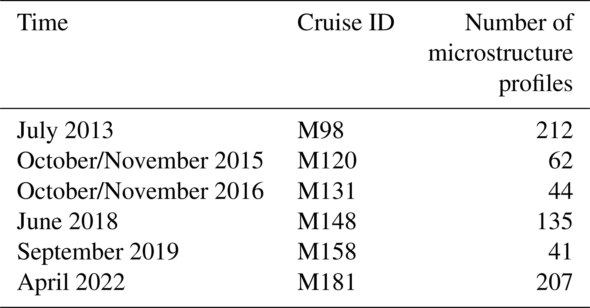
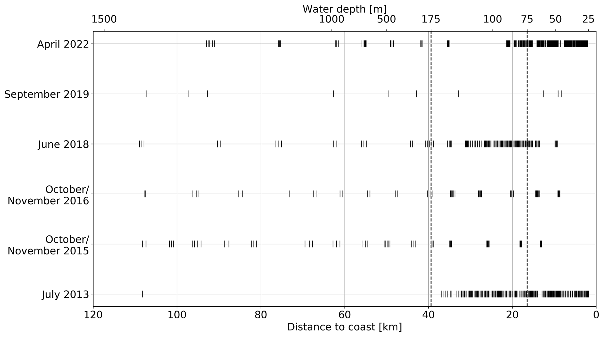
Figure 3 Distribution of microstructure profiles at the 11^∘ S section as a function of distance to the coast, cruise, and water depth. Each tick marks a microstructure profile. The vertical dotted lines mark the three areas analysed in Sect. 4.3: shallow water (water depth < 75 m), shelf break area (water depth > 75 and < 175 m), and deep water (water depth > 175 m).

2.2 Mooring data

We compare satellite data products of SST, near-surface horizontal velocities, and surface heat fluxes to data measured by a mooring at 6^∘ S, 8^∘ E (Fig. 1). The mooring is the Southeast Extension (SEE) of the Prediction and Research Moored Array in the Tropical Atlantic (PIRATA) programme. The PIRATA-SEE mooring was deployed for 1 year between June 2006 and June 2007. In June 2013 it was redeployed until September 2018. In March 2019 it was redeployed again for 6 months.

2.3 Satellite and reanalysis data

Different satellite and reanalysis products are used to estimate terms of the seasonal ML heat budget equation. As the datasets are available for different periods of time, we restrict our analysis to the time period between 1993 and 2018 for which all products mentioned below are available.

2.3.1 Surface heat fluxes

The climatologic net surface heat fluxes are derived from satellite data. Shortwave radiation and longwave radiation are taken from the TropFlux product (Kumar et al., 2012). The data are available on a $\mathrm{1}{}^{\circ }\times \mathrm{1}{}^{\circ }$ grid from 1979 to the present at a daily and monthly resolution. However, at the time when this study was conducted, only data until December 2018 were made available.

Latent and sensible heat fluxes are taken from the MERRA2 product (GMAO, 2008). The monthly mean fields are available on a 0.5^∘ longitude × $\mathrm{2}/\mathrm{3}$^∘ latitude grid from 1979 onward.

We chose to use different data products for the individual terms of the surface heat fluxes after comparing different data products to the surface fluxes measured by the PIRATA-SEE mooring (Appendix A).

2.3.2 Sea surface temperature

SST analyses are based on the OSTIA product (Good et al., 2020). The OISTA product uses satellite data as well as in situ measurements to provide global, daily, gap-filled SST fields. The data are available on a 0.05^∘ × 0.05^∘ grid from 1981 onward.

2.3.3 Surface velocities

Estimates of horizontal heat advection are based on near-surface velocities of the OSCAR (Ocean Surface Current Analysis Real-time) product (ESR, 2009). The OSCAR dataset derives near-surface ocean currents by using quasi-linear and steady flow momentum equations, thus combining geostrophic, Ekman, and Stommel shear dynamics. The basis is satellite and in situ measurements of sea surface height, surface vector wind, and SST. The data are available on a $\mathrm{1}/\mathrm{3}$^∘ × $\mathrm{1}/\mathrm{3}$^∘ grid with a temporal resolution of 5 d from 21 October 1992 onward.

2.3.4 Mixed layer depth

Mixed layer depth (MLD) is derived from the global Mercator Ocean reanalysis (GLORYS) product (Lellouche et al., 2021a). GLORYS is available daily from 1993–2019. It has a horizontal resolution of $\mathrm{1}/\mathrm{12}$^∘ and 50 vertical levels. We calculate the MLD using a temperature criterion, with the MLD defined as the depth at which the temperature deviates by 0.2 ^∘C from the surface value. MLDs determined from GLORYS were compared to the MLDs determined from PIRATA-SEE data as well as to MLDs calculated from the hydrographic Nansen dataset (Tchipalanga et al., 2018). The MLD calculated from the GLORYS dataset reproduces the observed MLD reasonably well (not shown).

3 Methods

3.1 Mixed layer heat budget

To assess the oceanic and atmospheric driver of heat content changes we calculate the ML heat budget by following the approach used by numerous previous observational studies (Stevenson and Niiler, 1983; Moisan and Niiler, 1998; Foltz et al., 2003, 2013; Hummels et al., 2014). The equation for the local heat balance in the ML can be expressed as

$$\begin{array}{}\text{(1)}& h\mathit{\rho }{c}_{\mathrm{p}}{\displaystyle \frac{\partial T}{\partial t}}=-\mathit{\rho }{c}_{\mathrm{p}}h\mathit{v}\cdot \mathbf{\nabla }T+q_{\mathrm{net}}+r,\end{array}$$

where h is the MLD, c_p is specific heat capacity, T the mean ML temperature, v the mean horizontal velocities in the ML, q_net the net surface heat flux corrected for the shortwave radiation that penetrates through the ML, and r the residual. Changes in the local heat content are balanced by the mean horizontal advection, the net surface heat flux, and the residual r. The residual contains errors of the terms of Eq. (1) and other processes. One of these processes, on which we will focus in the present study, is the heat loss due to turbulent mixing across the base of the ML, termed turbulent heat loss in the following. The influence of this term will be discussed based on estimates of mixing strength utilizing microstructure data collected during six cruises in the tAUS. However, the available data are not extensive enough to calculate a seasonal cycle of the turbulent heat loss. Other processes that are not evaluated here include the horizontal heat advection on temporal and spatial scales unresolved by the data used here (see Sect. 3.1.2), vertical temperature velocity covariance, and entrainment (Foltz et al., 2013; Stevenson and Niiler, 1983).

The evaluation of the terms of the ML heat budget is done using a box-averaging strategy. For that we consider two boxes (Fig. 1b). The coastal box includes the area from 8 to 15^∘ S within 1^∘ off the coast. The offshore box has the same latitude range and extends from the coastal box to 10^∘ E. All gridded terms are averaged spatially over the boxes. If a term of the ML budget consists of several variables with different spatial or temporal resolutions, we linearly interpolate the variable with the coarser resolution onto the higher-resolution grid. Furthermore, all gridded terms are averaged over the same time period (1993–2018).

3.1.1 Surface heat fluxes

The net surface heat flux consists of the sum of longwave and shortwave radiation as well as the latent and sensible heat fluxes. Shortwave radiation is corrected for the amount of radiation that penetrates through the ML while considering the absorption by phytoplankton. The vertical penetration of shortwave radiation can be estimated from climatological chlorophyll a concentrations. Morel and Antoine (1994) parameterize the irradiance at a certain depth by applying three exponentials. The first describes the absorption of the infrared parts of the sun spectrum depending on the angle of the incoming radiation. It decays on length scales between 0 and 0.267 m. The second and third exponentials express the absorption of the longer- and shorter-wavelength part of the visible spectrum. We find that only the third exponential is of interest for our application as the decaying scales of the first two exponentials are much smaller than the MLD. Thus, the fraction of shortwave radiation penetrating through the ML is

$$\begin{array}{}\text{(2)}& {\displaystyle \frac{E\left(-h\right)}{E\left(\mathrm{0}\right)}}\approx \left(\mathrm{1}-R\right)V_{\mathrm{2}}\exp \left[-{\displaystyle \frac{h}{Z_{\mathrm{2}}}}\right],\end{array}$$

where R=0.43 is the infrared part of the solar spectrum, and V₂ and Z₂ are polynomials of order 5 calculated with the monthly climatological chlorophyll a concentration and the constants given in Morel and Antoine (1994).

3.1.2 Mean horizontal heat advection

The mean horizontal heat advection is calculated using the OSCAR surface velocities and the horizontal gradient from the OISTA-SST product. Both the temporal and spatial resolution of the OSCAR surface velocities is coarser than that of the OSTIA SST. The OSCAR surface velocities are available with a 5 d resolution on a $\mathrm{1}/\mathrm{3}$^∘ × $\mathrm{1}/\mathrm{3}$^∘ grid. However, the OSTIA product also has limited effective resolution in the region of the Angolan Upwelling System. Due to persistent cloud cover in the area, high-resolution passive infrared SST data are rarely available and the SST retrieval largely has to rely on low-resolution (50–60 km) passive microwave data (Nielsen-Englyst et al., 2021). Thus, using these datasets we are not able to resolve horizontal heat advection on temporal scales shorter than 5 d and spatial scales smaller than passive microwave data resolution.

3.1.3 Turbulent heat loss at the base of the mixed layer

Turbulent heat fluxes are estimated from microstructure shear measurements. As the turbulent heat flux vanishes at the sea surface, its value across the ML base represents the turbulent heat flux divergence of the ML and thus the ML heat loss. The method used here to determine the turbulent heart flux is detailed in Hummels et al. (2014). A brief summary is provided below.

Data from airfoil shear sensors attached to microstructure probes are used to estimate dissipation rates of turbulent kinetic energy, ϵ, via the variance method while assuming isotropy. Through the integration of the shear wave number spectrum, $E_{\mathrm{d}u/\mathrm{d}z}\left(k\right)$ is related to the dissipation rate of turbulent kinetic energy as

$$\begin{array}{}\text{(3)}& \mathit{ϵ}=\mathrm{7.5}\mathit{\nu }{\int }_{k_{\min }}^{k_{\max }}{E}_{\mathrm{d}u/\mathrm{d}z}\left(k\right)\mathrm{d}k,\end{array}$$

where ν is the dynamic viscosity of seawater. The shear spectra are calculated from overlapping 2 s ensembles, which corresponds to ∼ 1 m vertical resolution. Subsequently, the spectra are integrated between a lower (k_min= 3 cpm) and higher wavenumber, k_max. The latter depends on the turbulence level and the noise level. To account for variance loss due to the limited resolution in wavenumber space, the spectra are fitted to the universal Nasmyth spectrum (Wolk et al., 2002).

The turbulent eddy diffusivity of mass is then calculated using (Osborn, 1980)

$$\begin{array}{}\text{(4)}& K_{\mathit{\rho }}=\mathrm{\Gamma }\langle \mathit{ϵ}\rangle N^{-\mathrm{2}},\end{array}$$

where Γ is the mixing efficiency (set to 0.2 following Gregg et al., 2018) and N² is the buoyancy frequency squared calculated from temperature, salinity, and pressure data recorded by the microstructure profiler. N² profiles were smoothed to vertical scales larger than the Ozmidov scale by using a least square fitting method to vertical property gradients. The window size is chosen depending on the distance to the ML, with 3 m directly below the ML increasing linearly to 30 m. Finally, the turbulent heat flux is estimated from $J_{\mathrm{H}}=-\mathit{\rho }{c}_{\mathrm{p}}{K}_{\mathit{\rho }}\partial T/\partial z$.

Turbulent heat fluxes are determined for each profile individually. For that, we change the vertical coordinate to MLD +Δz with a vertical resolution of 2 m. All measurements in the ML as well as 2 m below it are disregarded because mixing efficiency Γ is unknown in low-stratified waters (Gregg et al., 2018) and to avoid using data impacted by ship turbulence. Note that we do not interpolate the dissipation rates of TKE onto this grid but average all measurements in the respective depth bins. The binned profiles of dissipation rates of TKE are then used to calculate the turbulent eddy diffusivity and finally the turbulent heat flux for each profile. To evaluate the ML heat loss, all estimates in the depth range between 2 and 15 m below the ML are averaged. The use of this depth range is a trade-off between regions where we are able to estimate turbulent eddy diffusivities from microstructure data and statistical reliability of our results. Due to the lognormal distribution of the dissipation rates of TKE (e.g. Davis, 1996), it is desired to average many individual estimates of ε to increase statistical reliability.

3.2 Uncertainty estimation

The uncertainty of the monthly terms of the ML heat budget is calculated via ${\mathrm{err}}_{\mathrm{total}}=\sqrt{{\mathrm{err}}_{\mathrm{data}}^{\mathrm{2}}+{\mathrm{err}}_{\mathrm{seasonal}}^{\mathrm{2}}}$. The err_data term is the uncertainty arising from the data collection. To estimate the uncertainty of the satellite and reanalysis products for this region, we calculate the root mean square (rms) difference between the data and the data recorded by the PIRATA-SEE buoy. See Appendix A for the comparison of the individual variables used in the study. The seasonal error (err_seasonal) arises from the fact that we use a data record of finite length. It is the standard error of each month. The error of the terms of the ML heat budget calculated by combining different variables is calculated using standard error propagation.

To evaluate the uncertainty connected to the turbulent mixing we use the method of bootstrapping following the approach of Hummels et al. (2014). This method provides significance at the 95 % confidence level.

4 Results

Although the tAUS region is situated in the tropics, SSTs undergo an elevated seasonal cycle (Fig. 4a, b, d, e). The highest temperatures are found during austral autumn, reaching their maximum in March (Fig. 2, ∼ 28 ^∘C in both boxes). The lowest temperatures are observed during austral winter in August (Fig. 2, 20.9 ^∘C in the coastal and 21.5 ^∘C in the offshore box). Accordingly, the ML cools between March and August and warms during the rest of the year. In the following sections, we analyse the atmospheric and oceanic processes impacting the described heat content changes followed by an analysis of the resulting ML budget.

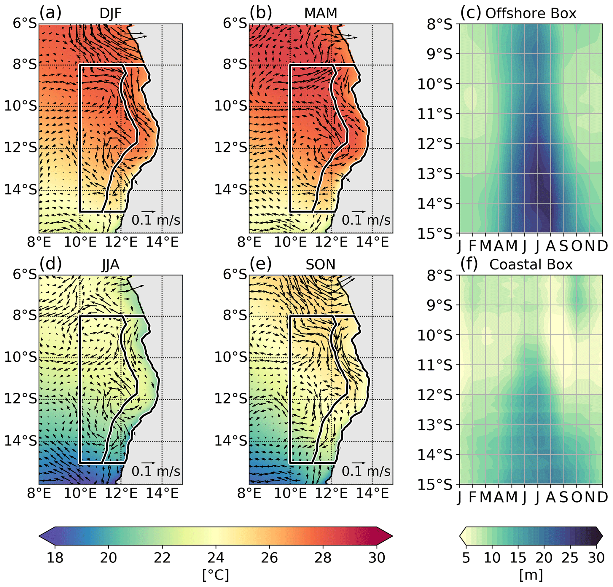
Figure 4 (a, b, d, e) Seasonal mean SST (colours) and surface velocities (arrows). The arrow length is referenced in the lower right corner of each panel. Black boxes show the coastal and offshore boxes used for calculating the ML heat budget. (c, f) Hovmöller plots of MLD as a function of latitude and month, zonally averaged over the (c) offshore and (f) coastal box.

Before turning to the individual processes, we look at the MLD and its changes throughout the year (Fig. 4c, f). In general, the ML is shallower near the coast than further offshore. Additionally, the ML deepens with increasing latitude. In both boxes the deepest ML is found in July when the average MLD is 12.7 m in the coastal and 22.9 m in the offshore box. The shallowest ML in the coastal box is present in January when it averages 6.2 m in the coastal box. In the offshore box, it reaches its minimum in February (8.1 m).

4.1 Surface heat fluxes

Surface heat fluxes show distinct seasonal cycles having similar characteristics in the offshore and the coastal box (Fig. 5). Differences between the boxes lie foremost in the amplitudes of the respective seasonal cycles. In both boxes, the incoming shortwave radiation peaks in January–February. The minimum in July is driven by the seasonal maximum in the solar zenith angle and the expansion of the low cloud cover (Scannell and McPhaden, 2018). The cloud cover is stronger further away from the coast (Zuidema et al., 2016), leading to higher incoming shortwave radiation over the coastal box. For the analyses of the ML heat budget, the amount of shortwave radiation that is absorbed within the ML is of interest. The fraction of shortwave radiation that is absorbed in the ML depends on the MLD and the chlorophyll concentration (see Sect. 3.1.1). This fraction is largest in austral winter when the MLD and chlorophyll concentrations are at their seasonal maxima (Fig. 5). On average the shortwave radiation absorbed in the ML is higher in the coastal box. The largest differences between the two boxes are observed in July when the ML in the coastal box receives 17 W m⁻² more shortwave radiation. The longwave radiation has its largest cooling effect in June. Between June and October, cooling by the longwave radiation is stronger in the coastal box compared to the offshore box. The latent heat flux has a similar seasonal cycle in both boxes. The smallest cooling effect is found between June and September when wind speeds are at their seasonal minimum. Latent heat flux cools the ML most strongly between February and May. Increased wind speed away from the coast (Fig. 1b) leads to an overall stronger cooling in the offshore box. The sensible heat flux is small in both boxes and constitutes a minor contribution to the net surface heat flux.

Figure 5 Climatology of surface heat fluxes averaged over the (a) offshore and (b) coastal box. The black dashed line shows the climatology of the incoming shortwave radiation (SWR), the black solid line of the SWR absorbed in the mixed layer, the orange line of the longwave radiation (LWR), the green line of the latent heat flux (LHF), the red line of the sensible heat flux (SHF), and the blue line of the net surface heat flux. Shaded areas give the uncertainty estimate of the respective fluxes (see Sect. 3.2).

The resulting net surface heat flux has its minimum in June and its maximum in September in both boxes. The difference in the individual surface heat flux terms results in a stronger net surface heat flux in the coastal box compared to the offshore box. Thus, the net surface heat flux acts to dampen the observed SST differences between the coastal and the offshore area. Consequently, the surface fluxes are not able to explain the signal of cold water in the near-coastal area of the tAUS. Note that the differences between the offshore and coastal box peaks between May and August when it is ∼ 30 W m⁻² stronger in the coastal box.

4.2 Mean horizontal advection

The seasonal cycle of the mean horizontal heat advection is determined by the seasonal cycle of the horizontal temperature gradient and the surface velocities (Eq. 1). Figure 4 shows that within the coastal box the temperature decreases towards the coast throughout the year. This negative zonal temperature gradient is strongest between May and August (∼ $\mathrm{12}\times {\mathrm{10}}^{-\mathrm{3}}$ K km⁻¹). A secondary maximum is found in January. In contrast, the meridional temperature gradient within the coastal box is always positive as SSTs increase towards the Equator. On average its magnitude is $\mathrm{5}\times {\mathrm{10}}^{-\mathrm{3}}$ K km⁻¹, while its seasonal cycle is weak. The meridional temperature gradient averaged over the offshore box is of similar strength (on average $\mathrm{5}\times {\mathrm{10}}^{-\mathrm{3}}$ K km⁻¹) and also exhibits a weak seasonal cycle. The offshore zonal temperature gradient is always positive as well (on average $\mathrm{3}\times {\mathrm{10}}^{-\mathrm{3}}$ K km⁻¹).

The velocity field off the coast of Angola is generally weak (Fig. 4). Close to the coast, velocities along the coast dominate. Here, the velocities in the northern part of the tAUS are elevated compared to further south throughout the year. The southward velocity component peaks in October (9 cm s⁻¹ averaged over the coastal box). Note that this maximum agrees well with the seasonal maximum of southward velocities of the Angola Current as shown from moored velocity observations in Kopte et al. (2017). A secondary southward velocity maximum is found in February. The weakest meridional velocities are found in August when velocities are close to zero. In the offshore box, the velocity field is weaker and noisier than in the coastal box. One feature present throughout the year seems to be an anticyclonic rotation centred around 12^∘ S, 12^∘ E. Averaged over the offshore box the surface velocities do not exceed 3 cm s⁻¹. Furthermore, annually averaged velocities are smaller than 1 cm s⁻¹.

The resulting mean zonal advection and meridional heat advection are presented in Fig. 6. In both boxes, the total mean horizontal heat advection is dominated by the meridional component. Averaged over the year, the mean horizontal heat advection warms the ML in both regions, but its contribution is small compared to the net surface fluxes. The maximum in both boxes is reached in October when southward velocities are at the seasonal maximum. Then, horizontal heat advection amounts to 18±3 W m⁻² when averaged in the coastal box and 7±3 W m⁻² for the offshore box. Note that mean horizontal heat advection is calculated using 5 d velocities available on a $\mathrm{1}/\mathrm{3}$^∘ grid. Heat advection on shorter timescales and smaller spatial scales cannot be determined from currently available datasets. This will be discussed in Sect. 5.

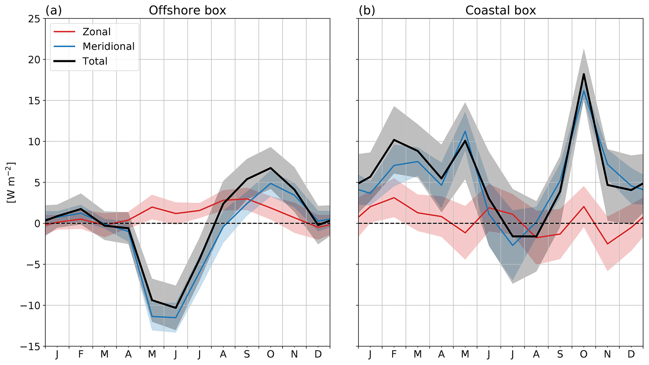
Figure 6 Seasonal cycle of mean horizontal heat advection averaged over the coastal box (a) and the offshore box (b). Red lines present the mean zonal horizontal heat advection, blue lines the mean meridional horizontal heat advection, and the black lines the sum of both. Shaded areas give the estimated error (see Sect. 3.2).

4.3 Turbulent heat loss at the base of the mixed layer

As has been reported from other upwelling regions (e.g. Perlin et al., 2005; Schafstall et al., 2010), the microstructure profiles available in this study (Sect. 2.1) indicate a strong dependence of the TKE dissipation rate on bathymetry. This is illustrated in Fig. 7, showing the mean distribution of TKE dissipation rates across the continental slope and shelf from six cruises at 11^∘ S (see Figs. 1b and 3 for details on data coverage).

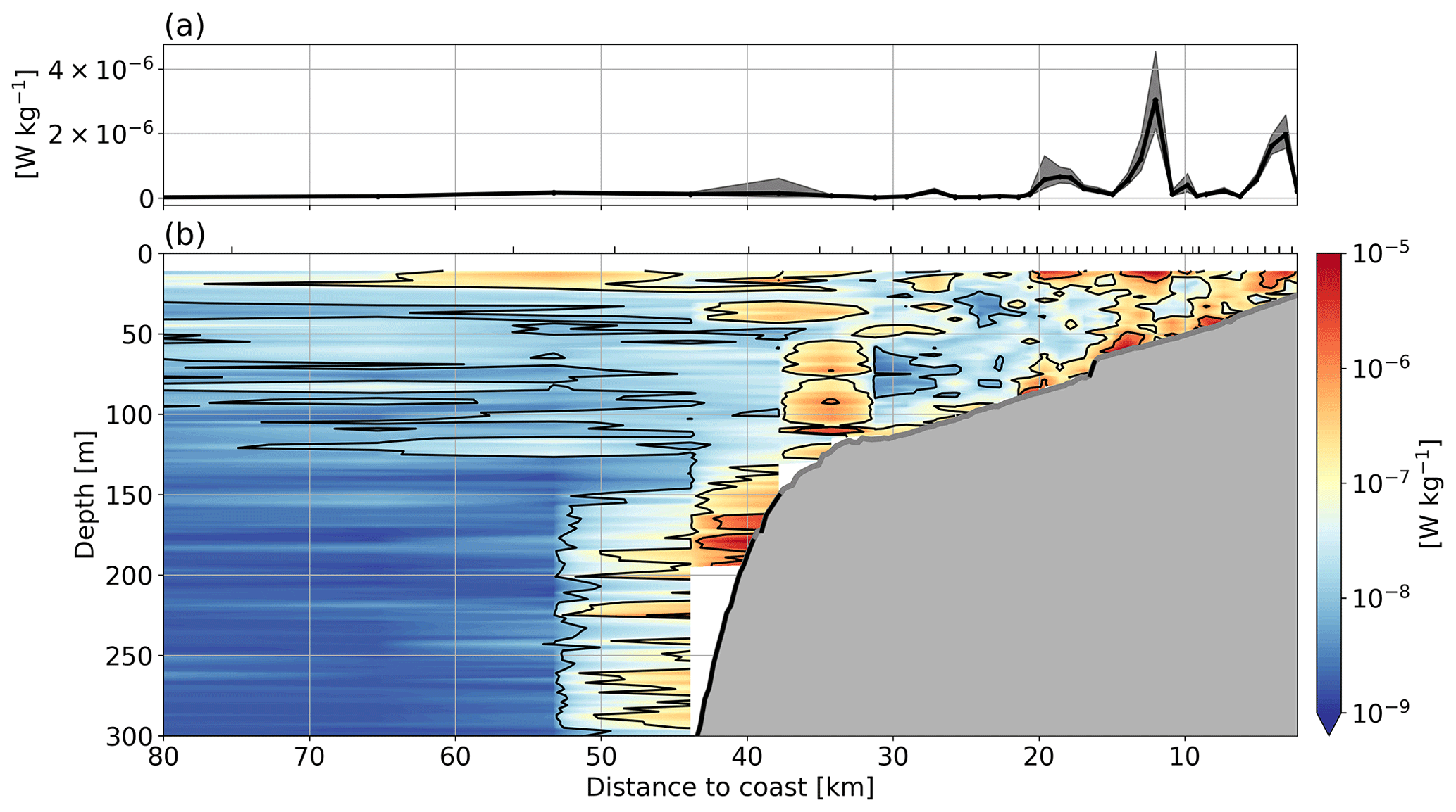
Figure 7 Dissipation of TKE at the 11^∘ S section (see Fig. 1b) as a function of distance to coast [km]. Microstructure data are binned together in groups of 20 profiles. (a) Mean dissipation of TKE averaged between 2 and 15 m below the ML. Grey shading shows 95 % confidence interval calculated via bootstrapping. (b) Section of mean dissipation of TKE against depth and distance to the coast. Topography coloured in black marks supercritical slopes for the M2 tide calculated with the time-averaged 11^∘ S stratification from Kopte et al. (2017). Black ticks at the top of (b) mark the borders of the 20-profile groups.

Elevated dissipation rates of TKE close to the surface as well as in and above the bottom boundary layer are revealed. Furthermore, dissipation rates above 10⁻⁷ W kg⁻¹ are found in the whole water column at the shelf break and in waters shallower than 75 m. In the depth range between 2 and 15 m below the ML (Fig. 7a), which is used to determine the turbulent heat loss at the base of the ML, a TKE dissipation rate dependence on the water depth is also evident. Here, elevated dissipation rates of TKE that can exceed $\mathrm{1}\times {\mathrm{10}}^{-\mathrm{6}}$ W kg⁻¹ are particularly frequent in waters shallower than 75 m. Note that the microstructure shear data were taken during different seasons. However, we find similar dependences of dissipation rates of TKE on water depth when considering data from individual cruises separately (not shown). Thus, the cross-slope distribution of TKE dissipation rates likely does not exhibit elevated seasonal variability.

We conclude from the mean distribution of dissipation of TKE that turbulent heat flux at the Angolan shelf has to be analysed dependent on the water depth of the respective microstructure profile. The 701 microstructure profiles were thus allocated into three groups based on water depth: profiles measured in water depths larger than 175 m (deep water), profiles measured in water depths between 75 and 175 m (shelf break area), and profiles taken in water depths shallower than 75 m (shallow water). Individual profiles were mapped as a function of vertical distance to the ML in 2 m bins prior to averaging (Fig. 8).

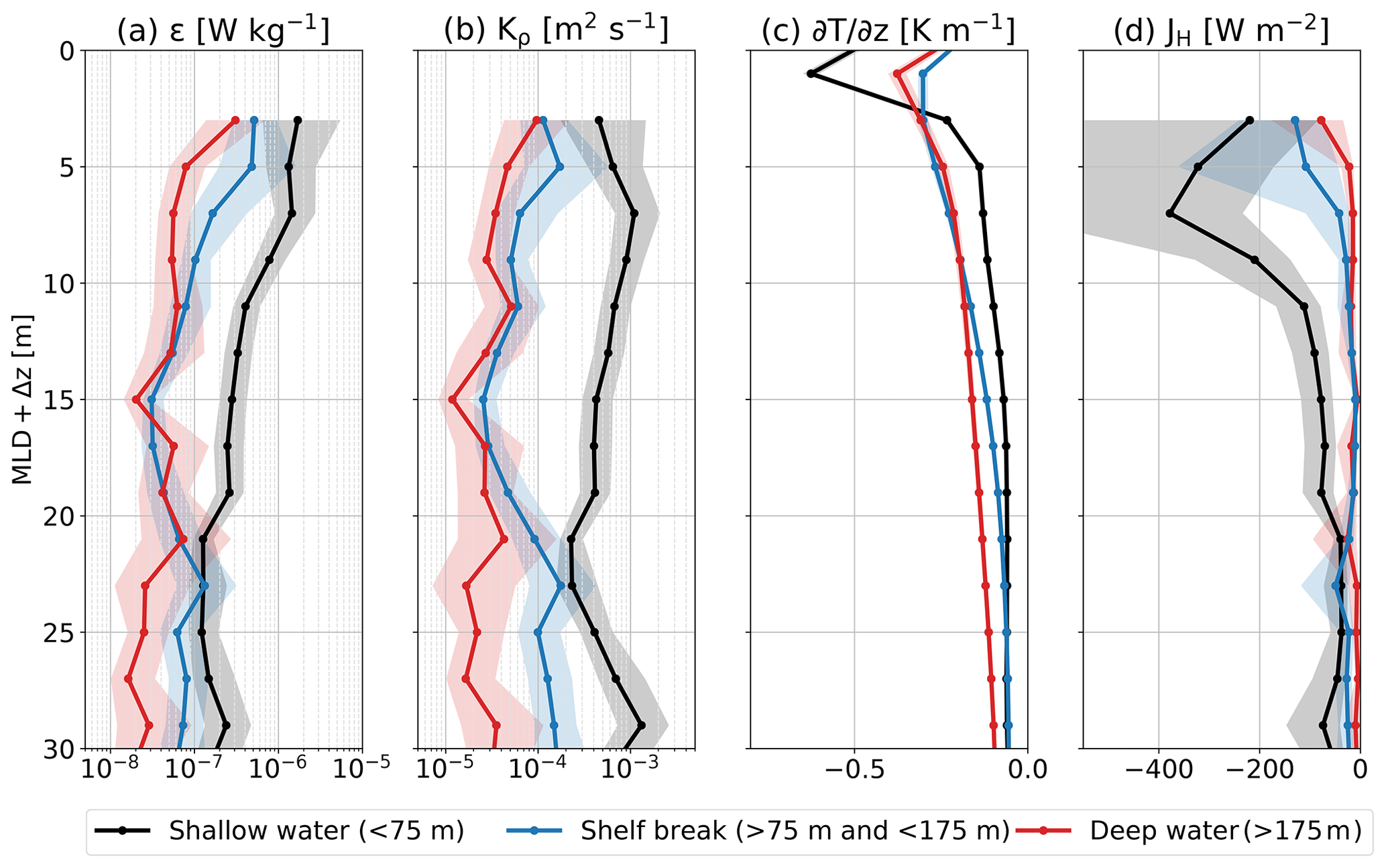
Figure 8 Averaged profiles as a function of distance to the ML. Profiles taken during six different cruises are allocated into three groups according to the water depth at which the profile was taken. Profiles taken in shallow water (water depth < 75 m, black), in the area of the shelf break (water depth > 75 and < 175 m, blue), and in deep waters (water depth > 175 m, red) are grouped together. (a) The dissipation rate of TKE [W kg⁻¹], (b) the eddy diffusivity [m² s⁻¹], (c) the vertical temperature gradient [K m⁻¹], and (d) the turbulent heat flux [W m⁻²]. The shaded areas give the 95 % confidence intervals.

The results in Fig. 8 clearly show differences between the three regions. The highest dissipation rates of TKE below the ML are found in shallow waters. These elevated dissipation rates of TKE ultimately lead to strongly elevated turbulent heat fluxes. Averaged between 2 and 15 m, the heat flux is −188 [−159, −222] W m⁻² in shallow waters (Table 2). In the same depth range, the shelf break area exhibits −49 [−42, −58] W m⁻². The heat loss in deep waters is even smaller (−24 [−21, −29] W m⁻²). These results show that turbulent heat loss at the base of the ML is an important cooling term of the ML heat budget. Here, the shallow waters play an especially important role as the heat loss is elevated by about a factor of 8 compared to deep waters.

Until now we have only discussed the turbulent heat flux as a function of bathymetry. For the analyses of the heat content change throughout the year, the seasonality of the turbulent heat flux is also of interest. It is ambitious to discuss seasonal differences of turbulent heat flux based on the cruise data. The sampling strategy during the cruises was not the same, leading to a different distribution of measured profiles along the 11^∘ S section during the different cruises (Fig. 3, Table 2). To discuss temporal variability, we present the averaged turbulent heat fluxes in the three different depth ranges between 2 and 15 m (see Sect. 3.1.3) during the different cruises (Table 2). The reported values clearly show large variability. In shallow waters, the fluxes range from −3 [−2, −3] W m⁻² (October–November 2015) to −390 [−326, −470] W m⁻² (April 2022). Similarly, in the area of the shelf break fluxes range from −2 [−1, −2] W m⁻² (October–November 2015) to −135 [−116, −163] W m⁻² (April 2022). In deep waters the minimum fluxes were measured during July 2013 (−1 [0, −1]) W m⁻²) and the highest were measured during September 2019 (−46 [−34, −64] W m⁻²). Note the variability between the two cruises conducted in October–November: in October–November 2015 an averaged flux of −3 [−2, −3] W m⁻² was measured in shallow waters, whereas 1 year later the average flux is −232 [−188, −290] W m⁻². Because of this large variability, we abstain from including seasonal estimates of turbulent heat flux at the base of the ML in the budget. A possible seasonality in the turbulent heat flux term is discussed in Sect. 5. Furthermore, the calculated fluxes from the microstructure data can exhibit very high values. The data recorded in April 2022 in shallow waters especially exhibit much higher heat losses than the amount of net surface heat flux put into the ML. In Sect. 5 we discuss a possible explanation for these high heat losses.

Table 2 Turbulent heat flux (J_H) averaged between 2 and 15 m below the ML during the respective cruise for profiles taken in different depth ranges. The 95 % confidence interval is given in brackets below. The number of profiles in each depth range is presented as well (N).

4.4 Mixed layer heat budget

Figure 9 presents the individual terms of the ML heat budget analysed in this study as well as the resulting budget itself averaged over the coastal and the offshore box, respectively. The net surface heat flux is an important term of the ML heat budget in both the offshore and the coastal box. In contrast, the mean horizontal heat advection term is small and of minor importance. Averaged over the year both terms have a warming effect on the ML in both boxes.

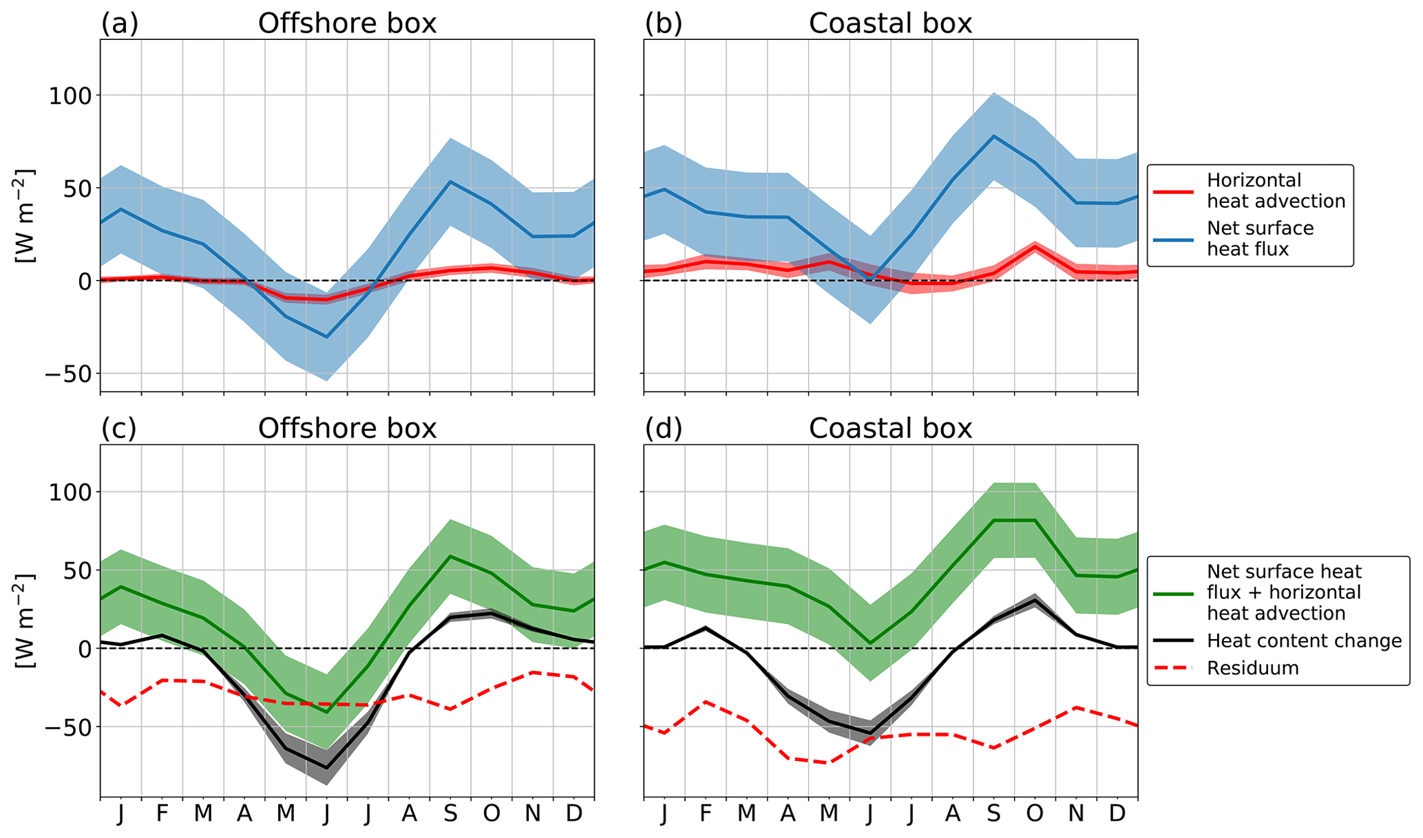
Figure 9 (a, b) Individual contributions to the ML heat budget. Colours are explained in the legend. (c, d) Sum of net surface heat flux and horizontal heat advection (green lines), the observed heat content change (black lines), and the resulting residuum between the two (red dashed line). Panels (a, c) show budget terms averaged over the offshore box, and panels (b, d) show budget terms averaged over the coastal box.

The sum of surface heat fluxes and mean horizontal heat advection shows a similar seasonal cycle with different magnitudes in the coastal and the offshore box (Fig. 9c, d). It is characterized by the seasonal cycle of the net surface heat fluxes and is only slightly modulated by the mean horizontal heat advection term. Consequently, the sum of the two is positive throughout the year in the coastal box. Its maximum is found in September (82±24 W m⁻²), while its minimum is found in June (3±24 W m⁻²). In the offshore box, the sum of net surface heat flux and total horizontal heat advection is negative between May and June. Its maximum is found in September (59±24 W m⁻²), and its minimum is detected in June ($-\mathrm{41}\pm \mathrm{24}$ W m⁻²). The heat content change reveals that the ML cools from March to August in both boxes. In austral winter, the heat content change is elevated in the offshore box compared to the coastal box. This may seem counter-intuitive given the increased negative SST gradient during this period but is explained by the deeper ML in the offshore box compared to the coastal box (Fig. 4c, f).

Comparing the heat storage term with the sum of mean horizontal heat advection and net surface heat fluxes reveals that a large residuum remains in the coastal box as well as in the offshore box (Fig. 9c, d). In the coastal box, the residuum is considerably larger (on average 53 W m⁻²). The average residuum in the offshore box is 29 W m⁻². The residuum undergoes a weak seasonal cycle which differs between the boxes. In the coastal box, the amount of the residuum has minima in February and November.

The residuum includes, amongst other things, contributions of the turbulent heat flux at the base of the ML. While we cannot calculate a seasonal cycle of this term for the coastal and the offshore box based on the microstructure data, an average contribution for the coastal box can be estimated. Analysis of the microstructure profiles revealed a dependence of the turbulence heat flux on bathymetry. Thus, we consider a weighted mean based on the area of the coastal box that falls into the respective depth ranges discussed in Sect. 4.3. In total, the water depth in 12 % of the coastal box area is shallower than 75 m, water depth in 13 % of the coastal box is between 75 and 175 m, and in 75 % it is deeper than 175 m. The resulting weighted mean calculated over all microstructure profiles averaged between 2 and 15 m below the ML yields a contribution of −48 [−43, −55] W m⁻² to the ML heat budget. Comparing this to the average residuum of 53±20 W m⁻² in the coastal box underlines the fact that turbulent heat loss at the base of the ML is an important process contributing to the cooling of the ML in the tAUS. The microstructure profiles further suggest that this process is particularly important in near-coastal areas as the turbulent heat flux is much larger there than further offshore. The larger residuum in the coastal box compared to the offshore box supports these results.

The residuum also includes biases in the evaluated terms of the ML heat budget (see Sect. 3.1). To estimate possible sources of biases, we compared the satellite and reanalyses data to in situ data measured at the PIRATA-SEE mooring site at 6^∘ S, 8^∘ E (see Fig. 1 for location). The comparison detailed in Appendix A revealed large differences in monthly averaged surface heat flux components despite being estimated over the same time span. In particular, the monthly averages of shortwave radiation showed elevated differences between the TropFlux climatology and buoy shortwave radiation sensor data, suggesting that TropFlux shortwave radiation is biased high. The differences in the net surface heat flux range between 2 W m⁻² in May and 38 W m⁻² in January. This suggests that the satellite and reanalyses data may overestimate the amount of net surface heat flux and thus contribute to a positive residuum in the ML heat budget.

5 Summary and discussion

The tAUS is a highly productive ecosystem. In the tAUS surface temperatures are lower near the coast compared to further offshore. In austral winter, we find the lowest SSTs and the strongest cross-shore SST gradient in the tAUS. In this study, we calculate different terms of the ML heat budget based on satellite and reanalysis data to analyse atmospheric and oceanic drivers of heat content variability. The heat budget terms are averaged over two boxes: one located directly at the coast of the tAUS and one offshore of it. This allows us to analyse and discuss processes that might be of different importance in both regions. Additionally, we analyse the impact of turbulent heat flux at the base of the ML based on shipboard observations taken almost exclusively in the coastal box.

The surface heat fluxes are an important driver of ML heat content changes in the tAUS. The seasonal cycles of the surface heat flux terms are similar near the coast and further offshore. The strongest cooling term is the latent heat flux, which is larger in the offshore area of the tAUS due to decreasing wind speeds towards the coast. As the warming due to shortwave radiation is elevated in the coastal region as well, the resulting net surface heat flux is larger in the coastal box compared to the offshore area. Thus, net surface heat fluxes act to dampen the observed cross-shore temperature gradient. Note that the differences are particularly large during austral winter when the cross-shore temperature gradient is at its seasonal maximum (Fig. 10).

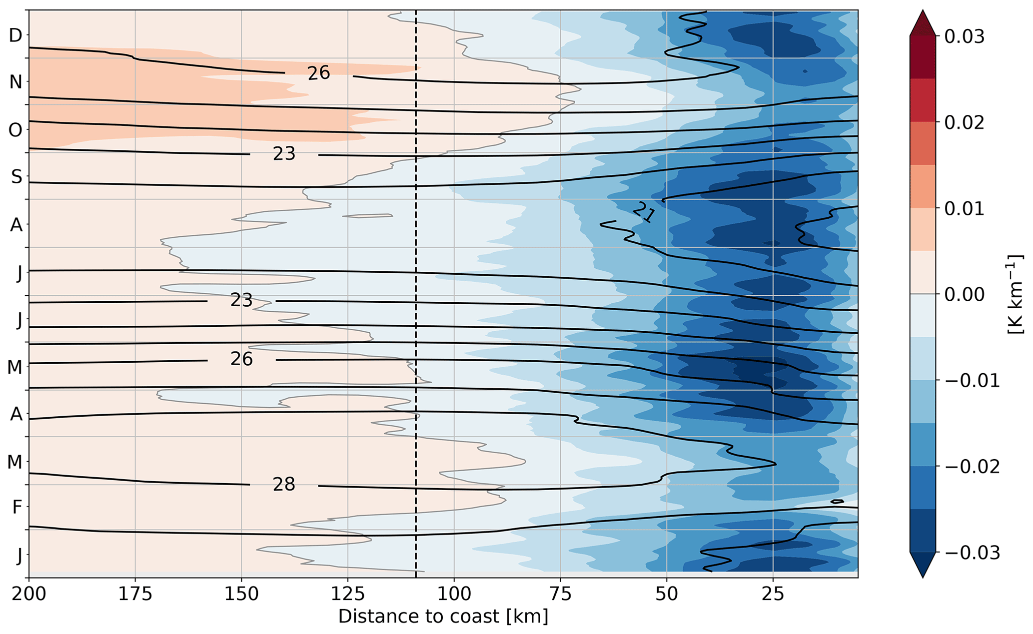
Figure 10 Zonal temperature gradient (colours) and SST (contours) as a function of distance to the coast averaged between 8 and 15^∘ S. Contour lines are every 1 ^∘ from 20 to 28 ^∘C. The black dashed line gives the approximate extent of the coastal box. The data are treated with a 5 d running mean.

The mean horizontal heat advection contributes to the warming of the ML in the coastal region as well as offshore. However, the term is small. It is sustained by the southward advection of warm equatorial waters by the Angola Current, which peaks during October.

The turbulent heat flux at the base of the ML is estimated from shipboard microstructure measurements taken during six cruises. We find the amount of heat flux to vary with bathymetry. The highest TKE dissipation rates and consequently elevated turbulent heat fluxes are found in water depths shallower than 75 m, suggesting stronger cooling close to the coast compared to further offshore. This term thus acts to enhance a cross-shelf temperature gradient.

The net surface heat fluxes and horizontal heat advection are not able to explain the observed heat content changes alone. Our analyses show that the turbulent heat flux at the base of the ML can explain a large proportion of the resulting residuum in the coastal box. The averaged residuum in the coastal box is nearly twice as large as in the offshore box, which supports the hypothesis that turbulent heat fluxes are more important near the coast compared to further offshore. Additionally, biases in the TropFlux surface heat fluxes may contribute to the residuum. As shown in the Appendix, shortwave radiation from the climatology is larger than that measured by in situ sensors on a PIRATA buoy situated in the proximity of the study site.

Our analysis of the ocean turbulence data reveals a connection between the amount of turbulent heat flux and bathymetry. Processes that lead to increased dissipation rates of TKE and ultimately increased turbulent heat fluxes in shallow waters on the Angolan shelf include internal waves and their interaction with the topography. Internal tides are assumed to be the largest contributor to the internal wave energy on the Angolan shelf (Zeng et al., 2021). They are generated by the interaction of the barotropic tide and the continental slope. In the tAUS, the topography is critical or supercritical with respect to the M2 tide at the continental slope mostly in the depth range between 200 and 500 m (Fig. 8, Zeng et al., 2021). Here, the largest portion of the internal tide energy is generated. While some of that energy was found to be dissipated locally or further offshore, a substantial amount propagates onshore and was found to be dissipated in shallow waters near the coast (Zeng et al., 2021). Note that smaller topographic features with critical slopes also exist further onshore, which can shape the local distribution of dissipation rates of TKE on the shelf as near-critical slopes are areas of enhanced velocity shear (Legg and Adcroft, 2003).

For the seasonal ML heat budget, the seasonality of turbulent heat flux at the base of the ML is of interest. The turbulent heat flux calculated from microstructure profiles exhibits high variability but also suggests that turbulent heat loss is an important cooling term throughout the year. However, the data only provide snapshots of the dissipation at the Angolan shelf. A robust discussion of seasonal differences based on the data is thus ambitious. The model study of Zeng et al. (2021) showed that seasonal variations in the spatially averaged generation, onshore flux, and dissipation of internal tide energy are weak. However, due to the seasonal variation in stratification (passage of CTWs, seasonal cycle of SSS, SST differences through surface fluxes) the mixing due to internal tides is more effective during austral winter when stratification is weak. The seasonality of the residuum of the ML heat budget presented in this study seems to support this result. The amount of the residuum averaged over the coastal box is smallest in February and November (Fig. 9) when stratification in the tAUS is strongest (Kopte et al., 2017). Furthermore, the results of Zeng et al. (2021) fit well to describe the increased cross-shelf temperature gradient during austral winter. Figure 10 shows the seasonal cycle of the zonal temperature gradient and SST as a function of distance to the coast. It reveals that the cooling and warming are not constant within 200 km distance to the coast throughout the year. Particularly, the zonal maximum of SST (zero contour line of the zonal temperature gradient, Fig. 10) is within the coastal box in some months and within the offshore box in other months. Note that temperature differences averaged over both boxes (Fig. 2) are thus not a perfect proxy for the cross-shelf temperature gradient. The strongest negative zonal temperature gradient is found between April and September with a secondary maximum in December–January. This increased gradient cannot be explained by the net surface heat flux. The difference between net surface heat fluxes in the coastal and the offshore boxes experiences its seasonal maximum in austral winter. Thus, the net surface heat flux acts to dampen the observed zonal SST gradient. The difference between the horizontal heat advection in the coastal and the offshore boxes is small. Furthermore, the seasonal cycle of this difference does not correspond to the seasonal changes in the zonal temperature gradient. Hence, the mean horizontal advection likely plays no role for the increased zonal temperature gradient in austral winter.

Summarizing, stratification changes connected to the passage of CTWs, the seasonal cycle of SSS, and the changing net surface heat fluxes likely influence how effectively the ML close to the coast is cooled by the dissipation of the internal tide, introducing a semi-annual cycle to the strength of the cross-shore temperature gradient. Nevertheless, the microstructure measurements suggest that the turbulent heat flux is an important cooling term throughout the year, setting up the negative cross-shore temperature gradient.

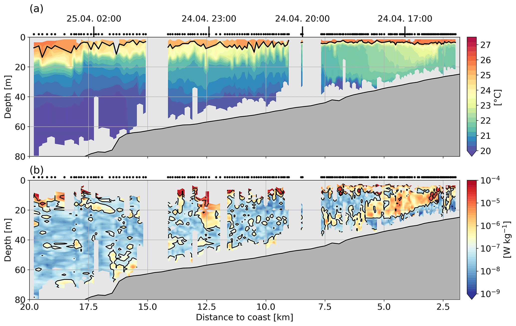
Figure 11 Shipboard section taken at 11^∘ S in April 2022. Panel (a) shows temperature (colours) and MLD (black line). Panel (b) displays the dissipation rate of TKE below the ML. Black points at the top of both panels mark the position of individual microstructure profiles.

The analysis and the turbulent heat flux calculated from the microstructure measurements revealed high variability between different cruises. The data collected in April 2022 show especially high fluxes (−390 W m⁻² in shallow waters). The influence of turbulent mixing on the temperature field can be seen in the transect measured on the shelf of Angola in water depths between 25 and 85 m (Fig. 11). The MLD decreased from around 7 m offshore to around 3 m towards the coast. The recorded section reveals strong internal wave activity as isotherms show strong undulation indicative of onshore propagating internal waves (Fig. 11a). This activity is primarily restricted to water depths larger than 50 m. In shallower water, internal waves do not appear anymore, suggesting the breaking of internal waves and dissipation of internal wave energy. It leads to high dissipation rates of TKE in this area with values mostly exceeding 10⁻⁷ W kg⁻¹. The effect of the enhanced mixing due to breaking internal waves on the temperature field is pronounced. Temperatures are vertically much more homogenous near the coast than in deeper water. The high dissipation rates in this area are not directly connected to the ML as a local minimum at around 10 m depth is detected. This suggests that the high mixing does not lead to a heat loss of the ML directly above. A very strong vertical temperature gradient of ∼ 1 K m⁻¹ below the ML supports the hypothesis that the mixing recorded here mostly affects the layer below the ML. Consequently, non-local effects have to play a role. Note in this context that the average heat loss in this area is estimated to be 390 W m⁻² (Table 2). This heat loss is higher than the heat input by the net surface heat flux and the mean horizontal heat advection. It implies that a one-dimensional view is not sufficient to understand the turbulent heat loss of the ML at the Angolan shelf. Horizontal advection on small spatial and temporal scales likely plays an important role in the redistribution of heat. Note that the model results of Zeng et al. (2021) reveal high spatial variability in dissipation at the Angolan shelf. This fits our results and ultimately suggests that strong mixing and thus strong cooling of the ML in the tAUS locally occur foremost in shallow areas and are redistributed by small-scale horizontal advection. Processes that could be important in this context are the heat advection by nonlinear internal waves (Zhang et al., 2015) and the influence of lateral eddy fluxes (Thomsen et al., 2021). Further work has to be conducted to understand the redistribution of heat on small temporal and spatial scales in the tAUS.

Seemingly contradicting our results, the study of Awo et al. (2022) showed that mean horizontal advection is an important term for the seasonal salinity budget. Their analysis shows that fresh water from the Congo River can reach 11^∘ S by meridional advection in February–March and in October–November. Note that we also find a peak in southward surface velocities in February and October. The velocities are also stronger in the northern tAUS until ∼ 11^∘ S (Fig. 3). However, as the meridional temperature gradient is weak in that region, the mean horizontal advection is not important for the local ML heat budget. Thus, the results of our study do not oppose the results found by Awo et al. (2022).

The results of the present study show that the residuum of the ML heat budget is likely explained by the turbulent heat loss at the base of the ML and the uncertainties in the net surface heat flux primarily in the shortwave radiation. The uncertainties in the net surface heat flux represent a shortcoming of the study. This is especially important as the tAUS is a region with a large SST bias in state-of-the-art climate models (Richter, 2015; Kurian et al., 2021; Farneti et al., 2022). One discussed reason for the bias is excessive shortwave radiation due to a poor representation of shallow stratocumulus clouds (Huang et al., 2007). Our results show that the uncertainty in shortwave radiation is seasonally dependent and higher in months when low-level clouds dominate (Scannell and McPhaden, 2018). This indicates that the correct representation of clouds in both models and observations is still an issue. It has to be resolved to get a better understanding of the tAUS and eastern boundary upwelling systems in general.

Summarizing, the study of the ML heat budget reveals that ML heat content changes in the tAUS are mostly determined by the surface heat fluxes and turbulent heat loss at the base of the ML. In contrast, the mean horizontal heat advection is of minor importance. The surface heat fluxes determine the seasonal cycle of heating and cooling of the ML and act to dampen the observed cross-shore temperature gradient. Turbulent heat loss at the base of the ML acts throughout the year in shallow waters of the tAUS. The microstructure data suggest that turbulent heat fluxes are capable of setting up the negative cross-shore temperature gradient. Stratification changes seem to control the amount of turbulent heat loss at the base of the ML, introducing a semi-annual cycle to the strength of the cross-shore temperature gradient.

Appendix A

A1 Comparison of satellite and reanalysis data to moored observation

For the calculation of the ML heat budget, we rely on satellite and reanalysis data. To discuss uncertainties for the different datasets we compare them to in situ measurements at the PIRATA-SEE mooring (6^∘ S, 8^∘ E). In the following, we will discuss uncertainties based on the time series of the different variables (Fig. A1) as well as on the seasonal cycle (Fig. A2). Here, the seasonal cycle of the satellite and reanalysis data is always calculated for the time period when the PIRATA-SEE data are available for the individual variables and interpolated on the mooring location. Note that the incoming shortwave radiation in the TropFlux product is multiplied by the factor 0.945 to account for the part of the radiation that is reflected at the sea surface (Kumar et al., 2012). To compare the different datasets, we multiplied the shortwave radiation measured by the PIRATA-SEE buoy and the MERRA2 data with the same factor.

Figure A1 Time series of variables (see titles of panels) of the ML heat budget at 6^∘ S, 8^∘ E from in situ data collected at the PIRATA-SEE mooring (black line) and from satellite and reanalysis data (colours, see legend). The daily PIRATA-SEE data are interpolated on the same time grid as the satellite and reanalysis data.

A1.1 Surface heat fluxes

The net surface heat flux is an important term of the ML heat budget in the tAUS as it is the largest warming term. From the time series, differences between data from the in situ fluxes measured by the PIRATA-SEE mooring and the surface fluxes from TropFlux and MERRA2 are recognizable (Fig. A1).

These differences are especially large for shortwave radiation. The shortwave radiation of TropFlux data always shows higher fluxes than the PIRATA-SEE data. In contrast, the shortwave radiation data from the MERRA2 product also exhibit lower heat fluxes than the in situ data. These differences become even more evident looking at the seasonal cycles of shortwave radiation calculated from the different data products. The PIRATA-SEE data reveal a maximum in shortwave radiation in February and a minimum in August. The seasonal cycle of the TropFlux data also shows a minimum in August. However, the maximum is found in January. The seasonal cycle also reveals that the TropFlux data record higher shortwave radiation throughout the year. Seasonal dependence of the differences is visible as they are smaller between March and July than during the rest of the year. The seasonal cycle of the MERRA2 shortwave radiation differs greatly more from the PIRATA-SEE data. The maximum is found in October and the minimum in April. Between June and December, the shortwave radiation of MERRA2 is larger than the shortwave radiation of PIRATA-SEE and vice versa during the rest of the year.

The other terms of the surface heat fluxes show better agreement between the different datasets. The seasonal cycles of the longwave radiation calculated from TropFlux, MERRA2, and PIRATA-SEE data are similar. However, offsets between the different datasets exist. The seasonal cycle of longwave radiation calculated from the TropFlux (MERRA2) reveals less (more) radiation compared to the PIRATA-SEE data almost throughout the year. For the latent heat flux the differences between MERRA2 and PIRATA-SEE are small (∼ 3 W m⁻²). The differences between TropFlux and PIRATA-SEE are larger (∼ 11 W m⁻²) with TropFlux showing less latent heat flux throughout the year. The contribution of the sensible heat flux to the net surface heat flux is in general small. Nevertheless, the seasonal cycle of MERRA2 is in better agreement with the seasonal cycle of the PIRATA-SEE data than the TropFlux dataset.

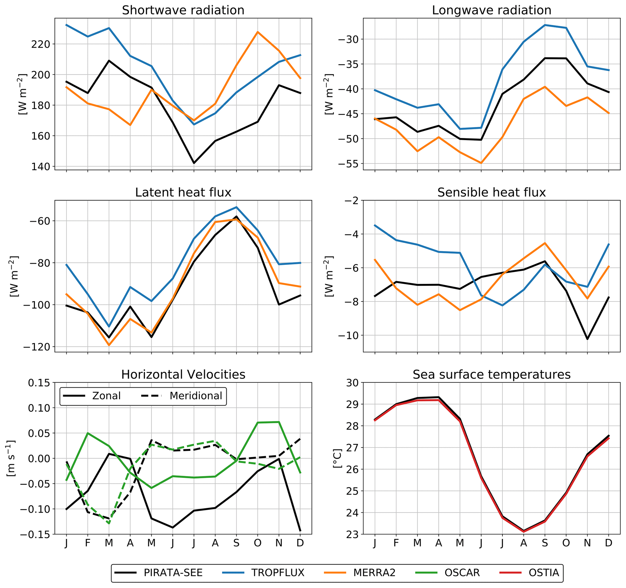
Figure A2 Seasonal cycle of variables (see titles of panels) used in the ML heat budget at 6^∘ S, 8^∘ E calculated from in situ data collected at the PIRATA-SEE mooring (black line) and from satellite and reanalysis data (colours, see legend). The seasonal cycle from the satellite data is derived from the time period when PIRATA-SEE data are available.

After considering the results of the comparison of the satellite and reanalysis data to PIRATA-SEE data we decided to use the TropFlux dataset for shortwave and longwave radiation and MERRA2 for latent and sensible heat flux for the ML heat budget. We based this choice on the smallest root mean square (rms) difference between the in situ data and the different satellite and reanalysis products.

The comparison between the climatologies of the TropFlux/MERRA2 and PIRATA-SEE data reveals a seasonal cycle in the differences between the different datasets. We want to investigate this bias by looking at the seasonal cycle of the mean differences between the time series (Fig. A3). The mean difference of shortwave radiation between the TropFlux product and the PIRATA-SEE measurements is higher than for the other heat flux terms and has a distinct seasonal cycle. Between July and February, the mean difference is higher (∼ 15 W m⁻²) than from March to June (∼ 5 W m⁻²). This seasonal cycle is most likely influenced by the seasonal prevalence of clouds of different types. Scannell and McPhaden (2018) show that at the PIRATA-SEE mooring site between January and April more high clouds than low clouds are present. This ratio is the other way around during the rest of the year. Note that the shortwave radiation measured by the PIRATA-SEE mooring is on average lower than what is measured by TropFlux, suggesting that the satellite data overestimate the amount of shortwave radiation. In contrast to the shortwave radiation, the latent and sensible heat fluxes provided by MERRA2 compare reasonably well with the turbulent fluxes measured by the PIRATA-SEE buoy. Similarly, the mean difference of longwave radiation between TropFlux and PIRATA-SEE data ranges 1–8 W m⁻² throughout the year. The bias of the net surface heat flux is dominated by the bias in shortwave radiation and ranges between 4 W m⁻² in April and 38 W m⁻² in January.

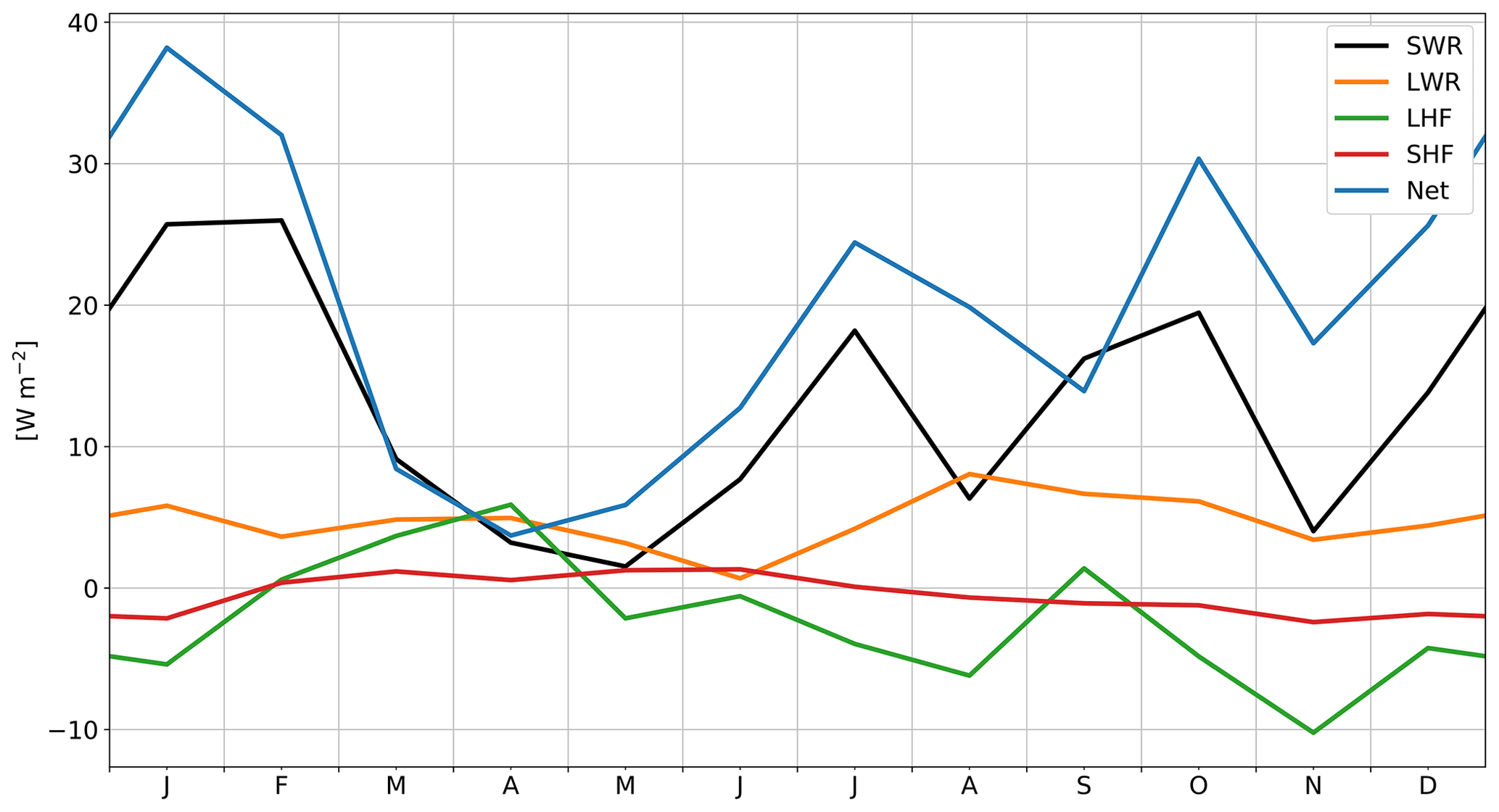
Figure A3 Climatology of the mean difference between the satellite and reanalysis data and the in situ measurements at the PIRATA-SEE mooring. For the shortwave (SWR) and longwave radiation (LWR) the TropFlux dataset is used, and for latent (LHF) and sensible heat flux (SHF) the MERRA2 dataset is used. The net surface heat flux (Net) is the mean difference of the sum of all fluxes between the satellite and reanalysis data and the in situ measurements.

Summarizing, comparisons of surface heat fluxes from different data sources show large uncertainties. The smallest differences are achieved using the TropFlux dataset for shortwave and longwave radiation and the MERRA2 dataset for latent and sensible heat flux.

To estimate the uncertainties of the sea surface heat fluxes for the ML heat budget we calculate the rms differences between the PIRATA-SEE and the satellite and reanalyses data from all available months. This rms difference of the shortwave radiation is 20 W m⁻², for the longwave radiation 6 W m⁻², for the latent heat flux 10 W m⁻², and for the sensible heat flux 2 W m⁻².

A1.2 Horizontal velocities

We compare the horizontal velocities measured at the PIRATA-SEE mooring at 10 m depth with the OSCAR velocities. The seasonal cycle of meridional velocities is similar in both datasets. A minimum southward velocity is found in March. During the rest of the year, the velocities are small. The rms difference based on monthly data is 7 cm s⁻¹. The seasonal cycle of the zonal velocities shows an offset of around 7 cm s⁻¹. The rms difference based on monthly data is 10 cm s⁻¹. Note that the zonal velocities show anomalous southward velocities during the end of the first mooring period (2007) that are much stronger than all other recorded data. Comparing only the latter mooring period to the OSCAR data reveals better agreement between the two datasets (not shown).

A1.3 Surface temperatures

The comparison between surface temperatures measured by the PIRATA-SEE mooring and the OSTIA SST product shows very good agreement. The rms difference between the two products based on monthly data is 0.1 ^∘C.