the Creative Commons Attribution 4.0 License.
the Creative Commons Attribution 4.0 License.
 | 22 Sep 2022
Import of Atlantic Water and sea ice controls the ocean environment in the northern Barents Sea
Øyvind Lundesgaard
Arild Sundfjord
Sigrid Lind
Frank Nilsen
Angelika H. H. Renner
The northern Barents Sea is a cold, seasonally ice-covered Arctic shelf sea region that has experienced major warming and sea ice loss in recent decades. Here, a 2-year observational record from two ocean moorings provides new knowledge about the seasonal hydrographic variability in the region and about the ocean exchange across its northern margin. The combined records of temperature, salinity, and currents show the advection of warmer and saltier waters of Atlantic origin into the Barents Sea from the north. The source of these warmer water masses is the Atlantic Water boundary current that flows along the continental slope north of Svalbard. Time-varying southward inflow through cross-shelf troughs was the main driver of the seasonal cycle in ocean temperature at the moorings. Inflows were intensified in autumn and early winter, in some cases occurring below the sea ice cover and halocline water. On shorter timescales, subtidal current variability was correlated with the large-scale meridional atmospheric pressure gradient, suggesting wind-driven modulation of the inflow. The mooring records also show that import of sea ice into the Barents Sea has a lasting impact on the upper ocean, where salinity and stratification are strongly affected by the amount of sea ice that has melted in the area. A fresh layer separated the ocean surface from the warm mid-depth waters following large sea ice imports in 2019, whereas diluted Atlantic Water was found close to the surface during episodes in autumn 2018 following a long ice-free period. Thus, the advective imports of ocean water and sea ice from surrounding areas are both key drivers of ocean variability in the region.
- Article
(17281 KB) - Full-text XML
- BibTeX
- EndNote


In the Atlantic sector of the Arctic Ocean, warm and saline water masses flow in from the North Atlantic and encounter colder, fresher water formed in the polar ocean. The meeting of ocean waters of Arctic and Atlantic origin is a fundamental feature of this region. The way in which these water masses spread and interact has major impacts on the distribution of a range of ocean properties and has wider effects on ecology, biogeochemistry, sea ice, and atmospheric climate. In the relatively shallow (∼50–450 m) Barents Sea, situated between the Arctic and the North Atlantic, most aspects of the natural environment are strongly shaped by its location at the intersection between these two ocean domains. Yet, many fundamental questions remain about the pathways of water masses in this region and the processes and dynamics that influence them – particularly in the less accessible northern region.
Atlantic Water (AW) is a relatively warm and saline water mass that flows into the Nordic Seas across the Iceland–Faroe–Scotland Ridge (Mauritzen, 1996; Hansen and Østerhus, 2000; Hakkinen and Rhines, 2009; Holliday et al., 2015). It travels northward along the Norwegian continental slope, and from there it enters the Arctic Ocean along two main pathways (Furevik et al., 2007; Aksenov et al., 2010; Beszczynska-Möller, 2011, see Fig. 1 of this paper). The first pathway is the Barents Sea Branch, by which AW travels through the southern Barents Sea (Loeng et al., 1997; Schauer et al., 2002; Ingvaldsen et al., 2002). There, it spreads and cools substantially and mixes with local water masses before entering the Eurasian Basin mainly through the St. Anna Trough in the Kara Sea (Schauer et al., 2002). The second pathway is the Fram Strait Branch, which continues northwards in the West Spitsbergen Current (WSC; Beszczynska-Möller et al., 2012). North of Svalbard, a fraction of the WSC turns eastwards and splits into three main sub-branches near the Yermak Plateau (Koenig et al., 2017; Crews et al., 2019). The branches crossing the Plateau ultimately converge to form the Fram Strait Branch of the Atlantic Water Boundary Current in the Arctic Ocean (FSAW), which flows eastward along the continental slope of the Nansen Basin (Woodgate et al., 2001; Pnyushkov et al., 2015; Våge et al., 2016). In contrast to the warm and saline AW are the “native” upper-ocean water masses originating in the Arctic Ocean, including its shelf seas. These water masses are commonly referred to as Polar Water (PW; Aagaard and Greisman, 1975; Rudels, 2015; Timmermans and Marshall, 2020) or Arctic Water (ArW; Mosby, 1938; Lind and Ingvaldsen, 2012; Oziel et al., 2016) – we will use the former term in this study. PW is formed through processes involving surface cooling and interactions with sea ice, meltwater, and AW, and it is generally characterized by being cold and relatively fresh. In addition, the surface layer in seasonally ice-free areas may be subject to surface warming in summer, resulting in warmer water masses distinguishable from AW by lower salinity.
The lateral distribution of ocean properties exerts a strong imprint on the Arctic ocean environment. The way in which water masses are layered in the vertical is also of fundamental importance to how the ocean interacts with the atmosphere and sea ice. In cold oceans, the density of seawater is dominated by salinity, and AW tends to sink below the colder but fresher PW. This results in a subsurface temperature maximum typically found at ∼150–250 m depth in large parts of the Arctic Ocean (Nansen, 1902; Coachman and Barnes, 1963; Timmermans and Marshall, 2020). The presence of a layer of PW atop the AW layer prevents oceanic heat from reaching the surface, thereby reducing the ocean heat loss, sea ice melting, and warming of the atmosphere (Renner et al., 2018). In the northern Barents Sea, the strength of the ocean stratification depends on the amount of sea ice that melts in the area (Lind et al., 2018; Aaboe et al., 2021): more meltwater yields a fresher PW layer, which in turn results in stronger stratification, limiting vertical mixing and upward heat fluxes from the AW layer. In the regions of strongest AW inflow – the southern Barents Sea, the WSC, and occasionally the upstream regions of the FSAW – this buffering PW layer is weak or non-existent, and AW typically extends to the surface, resulting in strong ocean–air heat fluxes with rapid cooling of the AW and warming of the lower atmosphere (Loeng, 1991; Ingvaldsen et al., 2021).
The Barents Sea is a region where the distribution of AW and PW has particularly striking imprints on large-scale ocean, sea ice, and atmospheric conditions. The Barents Sea has two clearly distinguishable domains – Arctic in the north and Atlantic in the south – separated by the Polar Front (Harris et al., 1998; Loeng, 1991; Oziel et al., 2016). The gradients between the northern and southern domains are sharpest in the western part of the Barents Sea, where the polar front is largely stationary (Harris et al., 1998). In the south, AW enters from the east through the Barents Sea Opening in large volume (∼2 Sv, Ingvaldsen et al., 2002; Skagseth, 2008) and occupies the entire water column. Here, the AW loses heat to the atmosphere and maintains the ocean ice-free and relatively warm through the winter (Mosby, 1962; Loeng, 1991; Schauer et al., 2002; Smedsrud et al., 2013). In contrast, the northern Barents Sea is cold, stratified, seasonally ice covered, and dominated by PW, with increased AW influence near the northern and southern bounds (Mosby, 1938; Loeng, 1991; Pfirman et al., 1994; Lind and Ingvaldsen, 2012). The north–south divide is also reflected in the ecological characteristics of the Barents Sea; substantial differences in food web structure and species composition largely reflect the underlying differences in the physical environment (Kortsch et al., 2015, 2019; Johannesen et al., 2017).
The Barents Sea is undergoing major, rapid ocean warming, with profound local effects on sea ice, ocean, and atmospheric conditions (Årthun et al., 2012; Smedsrud et al., 2013; Onarheim and Årthun, 2017; Barton et al., 2018; Lind et al., 2018). These changes in turn strongly affect ecosystem functioning and species composition in the area (Fossheim et al., 2015; Frainer et al., 2017; Dalpadado et al., 2020; Lewis et al., 2020). A fundamental change in the physical environment is the loss of sea ice in the north: despite the modest size of the region, nearly a quarter of the total Arctic sea ice area reduction in winter during the satellite era has occurred in the northern Barents Sea (Docquier et al., 2020, and references therein). The loss of sea ice has strong regional atmospheric climate effects (Ådlandsvik and Loeng, 1991; Smedsrud et al., 2013) and may affect weather in Eurasia through teleconnections (e.g. Petoukhov and Semenov, 2010; Li et al., 2018). Lind et al. (2018) documented that the ocean in the northern Barents Sea has experienced rapid warming, freshwater loss, and weakened stratification after 2005 and demonstrated a link between ocean warming, freshwater loss, and decreased sea ice import. More generally, sea ice loss in the Barents Sea and along the FSAW pathway is related to increased ocean temperatures and downstream progression of warmer waters, a process known as Atlantification (Årthun et al., 2012; Onarheim et al., 2014; Polyakov et al., 2017; Dörr et al., 2021).
It is well established in the literature that AW enters the Barents Sea from the north as well as from the west. Hydrographic surveys from the northern Barents Sea show a warming of deep (>100 m) waters towards the FSAW in the northernmost reaches of this region (Mosby, 1938; Loeng, 1991; Pfirman et al., 1994; Løyning, 2001; Lind and Ingvaldsen, 2012). While much of the northern shelf separating the FSAW from the northern Barents Sea is relatively shallow, regional model simulations (Aksenov et al., 2010; Lind and Ingvaldsen, 2012; Athanase et al., 2020) have indicated that modified AW enters through deep (>250 m) troughs that cut across the northern shelf from the continental slope into the northern Barents Sea: the wide Franz Victoria Trough and the narrower Kvitøya Trough (Fig. 1). The model results are consistent with in situ observational evidence of AW in these troughs (Mosby, 1938; Matishov et al., 2009; Pérez-Hernández et al., 2017). Both observational (Matishov et al., 2009; Pérez-Hernández et al., 2017) and model studies (Athanase et al., 2020; Menze et al., 2020) suggest a circulation pattern within the troughs, with southward AW inflow on the western side and a return flow of colder and fresher waters on the eastern side.
The variability of ocean transport into the northern Barents Sea from the north is not well known. Aagaard et al. (1981) presented a year of point current meter data from a mooring in the centre of Kvitøya Trough, finding a weak northeastward mean flow. While this study was mainly focused on tidal dynamics, the authors noted occasional episodes of intensified northward currents during the passage of cyclones over the Barents Sea. Sternberg et al. (2001) showed a 5-month record of near-bed currents measured by a bottom tripod in Olgastretet southwest of Kong Karls Land in 1991–1992. They observed flows that were frequently strong enough to resuspend sediment and frequent reversals of the near-bed currents over periods of 3 to 8 d. Temperature records from 75 m depth shown in Aagaard et al. (1981) appear to indicate a seasonal cycle, with maximum temperatures observed in January, and general circulation model simulations have indicated maximum mid-depth temperatures in the northern Barents Sea during autumn (Lind and Ingvaldsen, 2012). The FSAW itself undergoes a seasonal cycle in both currents and hydrography, with stronger inflow and a broader and warmer AW core north of Kvitøya from late autumn into early winter (Ivanov et al., 2009; Renner et al., 2018; Lundesgaard et al., 2021). Long-term repeat hydrographic profiles collected in the northern Barents Sea in autumn show substantial temperature variability also on interannual timescales; year-to-year variations in both wind stress forcing north of Svalbard (Lind and Ingvaldsen, 2012) and sea ice import from the north and east (Lind et al., 2018) have been proposed as important mechanisms for interannual variations in salinity and temperature.
A recent summary of the physical and ecological impacts of Atlantification in the Barents Sea sector of the Arctic Ocean (Ingvaldsen et al., 2021) highlights the need for regional observational studies along advective pathways in order to better understand the ongoing system-wide changes. The Barents Sea has been monitored extensively for half a century, with annual hydrographic surveys since the 1960s, but the current knowledge about the northern Barents Sea ocean climate is largely based on ocean profiles from the ice-free area in August–September. Ocean observations below the sea ice are sparse, and the seasonal hydrographic variability is largely unknown. The goal of this study is to document the seasonal evolution of currents and water properties at northern inflow regions of the northern Barents Sea. While the observational records that are presented contain many interesting features that may each merit attention, we restrict our main focus here to the following questions.
-
How and why do ocean temperature and salinity vary through the year?
-
What characterizes ocean circulation on the northern margin of the northern Barents Sea, and what forcing mechanisms drive the flow?
-
What role do advective imports of Atlantic Water and sea ice, respectively, play in setting the seasonal hydrography of the northern Barents Sea?
To this end, we present unique long-term time series of nearly continuous ocean measurements from the northern Barents Sea from two different ocean moorings deployed from autumn 2018 to autumn 2020. The moorings were located downstream of the two deep troughs assumed to be “gateways” of AW transport to the Barents Sea from the north (based on topographic steering and the model simulations cited above). This paper contains a detailed description of the evolution of the hydrography and currents at the mooring sites, providing important environmental context for studies of the northern Barents Sea across disciplines. The observations allow us to offer an interpretation of the circulation of AW into the northern Barents Sea based in the mooring observations combined with shipboard cross-slope conductivity–temperature–depth (CTD) transects. We analyse time series of sea ice concentration, sea level pressure, and wind stress curl in order to examine drivers of the observed ocean variability, establishing a correlation on intermediate timescales between inflow from the north and regional wind forcing due to synoptic weather systems passing through the Barents Sea. While the dynamics governing this interaction are beyond the scope of the study, we discuss possible mechanisms by which atmospheric forcing may directly or indirectly impacts the ocean in the northern Barents Sea. This study aims to fill considerable observational knowledge gaps, contributing towards a more complete understanding of the physical ocean environment of the northern Barents Sea. This is crucial for understanding ongoing processes and changes in the northern Barents Sea itself, but it is also relevant for other Arctic shelf seas, which may come under increasing influence of Atlantic Water in coming decades.
2.1 “Northern gateway” ocean moorings
We examine the records from two ocean moorings, M1 and M2, that operated in the northern Barents Sea during two consecutive deployments between October 2018 and September 2020 as part of the Nansen Legacy project's observational programme. The moorings were positioned at sites of sloping bathymetry downstream of the troughs assumed to be “gateways” of ocean transport into the northern Barents Sea from the north and east (Fig. 1). M1 (western mooring) was located at 79∘35.4′ N, 28∘5.8′ E, directly downstream of Kvitøya Trough. M2 (eastern mooring) was situated at 79∘40.7′ N, 32∘19.2′ E, a location chosen in order to capture inflow from Franz Victoria Trough some 150 km to the east.
Both moorings were deployed during the KPH2018710 Nansen Legacy Paleo Cruise in October 2018 and recovered during the KPH2019710 Nansen Legacy and A-TWAIN/SIOS-InfraNor Mooring Service Cruise in November 2019. During this same cruise, the moorings were redeployed with a different set of instruments. Both moorings were recovered in October 2020 on the KPH2020706 cruise led by the Institute of Marine Research. All three mooring cruises were on RV Kronprins Haakon. We will refer to the individual mooring deployments as, e.g. M1–2 (M1 mooring, second deployment).
Both moorings were equipped with one upward-looking RDI Teledyne 150 kHz acoustic Doppler current profiler (ADCP) mounted near the bottom, one upward-looking Nortek Signature 500 kHz ADCP mounted within the upper ∼30 m, and RBR Concerto conductivity–temperature–pressure (CTP) and RBR Solo temperature sensors at various points along the mooring line. Tables 1 and 2 show the exact locations, sensor configurations, and deployment dates of the moorings.

Figure 1(a) Map of the Svalbard region, indicating the West Spitsbergen Current (WSC) and its major branches entering the Arctic Ocean and recirculating in the Fram Strait (orange arrows). White and black contours show the 2000 and 250 m isobaths. (b) Closer view of the study area in the northern Barents Sea showing positions of M1, M2, and AT800 moorings (red symbols); shipboard CTD transects (dotted black lines); and weather stations (stars) used in this study. Bathymetry from IBCAO v3 (Jakobsson et al., 2012).
2.1.1 Moored CTD instruments
Physical variables were computed from raw Solo and Concerto data using the RBR Ruskin software (version 2.12.13). Sensors were laboratory calibrated before and after deployment, and the final data were obtained by assuming a linear drift from pre- to post-deployment calibration time series, in general yielding small corrections within the manufacturer's specified accuracy.
One Concerto sensor on M1–1 (∼170 m depth) experienced a cracked conductivity cell and showed relatively large (2.1 db) difference in pressure calculated from pre- and post-deployment calibration. Salinity from this instrument was rejected from the analysis, and after examining the on-deck pressure record, only pre-deployment calibration coefficients were used to compute pressure. Another Concerto sensor on M1–1 (∼250 m depth) experienced issues related to depletion of the battery near the end of the record, and the data were rejected after 8 November 2019 as a result, shortening the record by 8 d. No data are available from a near-bottom Concerto on M2–1 (flooded) or from Solo instruments near 60 m on both M1–2 (lost instrument) and M2–2 (did not record).
Obvious spikes in conductivity were removed during manual inspection, and a 25 min window median filter was applied to all records of practical salinity. Sensor values generally compared well with shipboard conductivity–temperature–depth (CTD) profiles collected near deployment and recovery, although the large temporal variability prevented a detailed comparison of values below the mixed layer. For one Concerto located in the mixed layer on M2–1 (near 19 m, where water properties were relatively stable), comparison with shipboard CTD at recovery indicated artificially low measured conductivity. We applied a drift factor to the measured conductivity from this sensor, linearly increasing through the melt season (from 15 June 2019) to match the CTD profile at recovery on 17 November 2019, yielding a maximum change in practical salinity of 0.056 at the end of the record. Salinity variations on this scale measured by near-surface Concertos should be interpreted with caution; however, the signals discussed in this study are generally of greater magnitude.
For RBR Concertos, depth and absolute salinity (SA), conservative temperature (Θ), and potential density anomaly at 0 db (σ0) were calculated using the GSW-Python package (https://github.com/TEOS-10/GSW-Python, last access 12 October 2020). For the Solo instruments, which did not have pressure sensors, instrument depths were estimated based on adjacent Concertos. The offset from planned Solo depth was obtained by interpolating between the offsets of Concertos above and, where available, below. For the bottom Solo instrument on M2–1, where no functioning Concerto was present below, an additional offset of 8.3 m was applied to the Solo depth record based on comparison with the recovery CTD profiles, reducing the deviation between median and planned depth for this sensor to 4.1 m. These depth estimates for the Solo instruments are approximations; in many cases, the deviation between planned and observed Concerto depth was large (up to 16 m) and varied along the mooring line. We have no information about where on the mooring these depth offsets originated, and the true depth of the Solo sensors are therefore not known exactly. In this paper, we have used the best depth estimates described above, but we also suggested a range of these estimates bounded by the depth deviations of adjacent Concertos (Table 1). Neither the visual impression of figures including the Solo data nor the quantitative results where they are included are sensitive to the exact position of these sensors within the estimated depth ranges. We are therefore confident that the uncertainty in depth of the Solo instruments did not impact the results and conclusions presented in this study.
2.1.2 The 500 kHz upper-ocean ADCPs
Upward-looking Nortek Signature 500 kHz five-beam ADCPs (Sig500s) were mounted in the top buoys of the moorings. Data averaged from sampling over 52 s cycles every 15 min were used to generate a time series of near-surface ocean currents computed from the four slanted beams. Data were converted to physical variables using Nortek's SignatureDeployment software, and further post-processing was applied to the average profiles.
Transducer depth and bin depths were calculated from sea pressure using GSW-Python after removing a fixed atmospheric pressure. Small corrections of <1 dbar were applied to the sea pressure record from requiring zero sea pressure at recovery to be ∼0 dbar. This nudged the offset from nominal depth toward that of nearby RBR Concertos and improved the match with the depth measured by the Sig500 centre “altimeter” beam during ice-free periods.
Measurements collected during deployment and recovery were identified from the pressure record and removed. Some individual current measurements were rejected based on a number of successive criteria for variables including backscatter amplitude, beam correlation, current speed, and instrument tilt. Measurements where bin depth was shallower than 10 % of the transducer depth were also rejected to avoid side lobe interference near the surface. Lastly, the current vector was rotated to correct for time-dependent magnetic declination, calculated using the geomag python module (https://pypi.org/project/geomag/, last access: 11 May 2021), which uses the 2015 World Magnetic Model (Chulliat et al., 2014, mean declination angles: M1–1: 19.1∘; M1–2: 19.5∘; M2–1: 22.2∘; M2–2: 22.6∘).
Table 1Overview of moorings M1 (a, b) and M2 (c, d) with deployment dates and locations and depths of moored CTP instruments. Concerto stands for RBR Concerto (CTP), and Solo stands for RBR Solo (T). Median depth is calculated from pressure after removing deployment and recovery. For the Solos, depth was assigned based on interpolation between adjacent Concertos with pressure sensors (and comparison with CTD profile in the case of the bottom Solo on M2–1; see Sect. 2.1.1). The range column shows the estimated range of the median depth of RBR Solos.
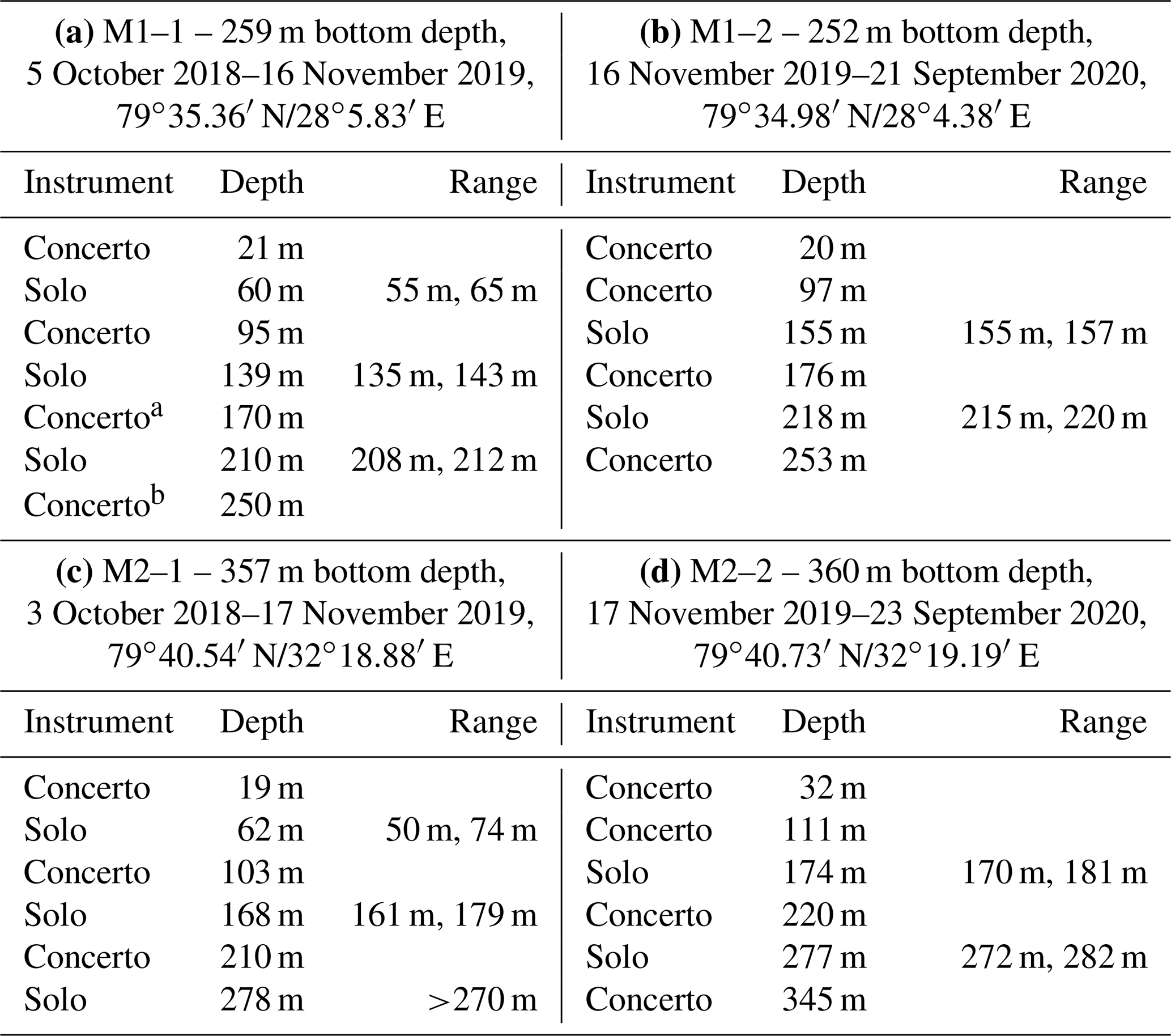
a Suspect conductivity data only using pressure and temperature. b The record from this instrument ends on 8 November 2019.
2.1.3 The 150 kHz water column ADCPs
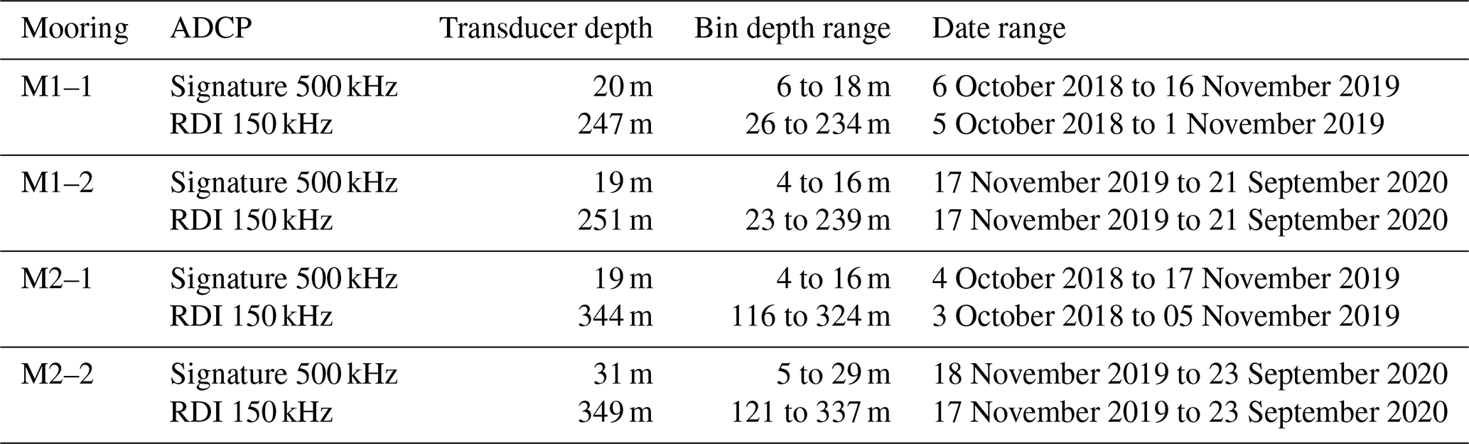
RDI Teledyne 150 kHz ADCPs (RDI150s) were mounted near the bottom of the mooring and looking upward. All RDI150s were configured with a bin size of 8 m, obtaining current profiles from ensembles every 20 min (50 acoustic pings per ensemble, 24 s per ping). RDI150 data were converted to physical units using RDI's WinADCP software. Fixed depth offsets were applied to the pressure sensor-derived transducer depth and bin depths, assuming that the differences between nominal and observed depth should be the same as those of nearby Concerto pressure sensors. These depth corrections amounted to −2.3 m for both M1–1 and M1–2 and +3.2 m for M2–2. The RDI150 on M2–1 had no functioning Concerto nearby, and so no fixed offset was applied to its depth record. However, a clear linear drift of 1.24 m yr−1 was found in the depth record from this instrument, which was therefore detrended assuming initially true values.
Bins with median depth located within the last 6 % of the distance between the instrument and the surface were removed in order to avoid side lobe interference (this only affected M1–1). Profiles collected during deployment and recovery were also removed.
The RDI150 records from the first deployment were cut short by 16 d (M1–1) and 12 d (M2–1) due to battery depletion near the end of the record and associated data glitches in the period before recording ceased.
Further post-processing was applied to the RDI150 velocity data, involving a number of successive tests where measurements outside accepted ranges were rejected. Two adjoining mid-depth bins at M1–2, near 103 and 111 m depth, were suspected to be affected by reflection of mooring elements and therefore removed from the record. The same was the case for one near-surface bin that was removed at M1–1. A time-varying clockwise rotation of ∼20∘ was applied to horizontal currents from the RDI150s in order to correct for local magnetic declination, using the same procedure as described for the Sig500 data.
The flux gate compasses of the RDI150s were factory calibrated before the first deployment. Before the second deployment, the RDI150s were equipped with new batteries, but no new calibration was performed. This, along with possible compass errors resulting from interference from magnetic elements on the buoy, prompted a closer investigation of the records of instrument heading and current direction. This investigation revealed significant deviations from expected current direction based on bathymetry, upper-ocean currents measured by the Sig500s, and the Arc5km2018 tidal model (Erofeeva and Egbert, 2020). In particular, mean and tidal currents measured at M2–2 were oriented ∼70∘ clockwise of the expected direction and of the direction measured during M2–1. Compass direction issues are a frequent concern for ADCP current measurements (which are sensitive to compass heading) and pose an especially major challenge at high latitudes where the horizontal magnitude of the Earth's magnetic field is weak. As a corrective measure, we adjusted RDI150 current directions based on the observed relationship between the currents measured in the upper bins of the RDI150s and those measured by the overlying Sig500s, which were equipped with solid-state magnetometer compasses and exhibited more consistent current records. The method was based on von Appen (2015), who applied a heading-dependent correction based on a best-fit relationship between current directions measured by moored ADCPs and fixed-point current meters on the same moorings. We compared current directions from the upper RDI150 bins with those from the Sig500s, extracting a relationship between the two as a function of the heading of the RDI150 instrument. Only data from periods of near-full ice cover (and weak vertical gradients) were included in the comparison. A best fit to the direction difference between the RDI150 and Sig500 currents was extracted using non-linear least squares weighted by current speed, assuming the functional shape of a single-period sinusoid with an offset. The extracted heading-dependent current direction offset was then applied to the entire record of horizontal currents from the RDI150. This procedure visibly improved the records at the M1 mooring, where the RDI150 and Sig500 ranges were separated by <10 m and the heading-dependent direction difference exhibited a clear sinusoidal shape. At M2, the RDI150 and Sig500 ranges were separated by >100 m and the relationship between the two instrument records was noisier. Yet, the correction clearly improved the match between M2–2 mean currents and the local bathymetric slope, between M2–2 tidal currents and Arc5km2018 predicted tides, and between M2–1 and M2–2 currents overall.
Table 2Overview of M1 and M2 mooring ADCP instruments: Nortek Signature 500 kHz ADCPs and RDI 150 kHz ADCPs. The transducer depth column shows median depth based on instrument pressure records. For RDI150s, depths have been adjusted to nearby RBR Concerto records as described in Sect. 2.1.3. The bin depth range column shows the median depth of the deepest and shallowest bins after processing. The date range column shows the time range from which data are available.
Although we are confident that these corrective measures markedly improved the RDI150 current directions, uncertainties are large in the case of M2. While we have no procedure to rigorously estimate true errors, we believe the direction of RDI150 currents measured at M1 to be a good representation of the true flow direction. The error is greater for M2–1, which had a recent calibration but could only be compared directly with currents further up in the water column. The greatest uncertainties are associated with M2–2, where we lack a compass calibration after the battery change and have applied relatively large corrections to the compass data. The RDI150 records from M2 should therefore only be used to indicate the current direction in a very general sense.
2.1.4 Interpolation and filtering
All variables were linearly interpolated onto equal grids in time and depth for analysis and plotting. All currents shown in this paper have been filtered in time using a 40 h seventh-order Butterworth filter before further analysis in order to focus on the subtidal component of the flow.
2.2 Slope current mooring
In order to compare the seasonal evolution in the northern Barents Sea with the AW slope current north of Svalbard, we used ocean current and temperature data from the AT800 mooring, which was located on the slope north of Kvitøya at 81∘32.9′ N, 31∘52.3′ E, as part of the A-TWAIN mooring array (Renner et al., 2018), which has been in place with a varying number of operational moorings since 2012. The AT800 mooring was located at a water depth of approximately 880 m, near the core of the FSAW (Fig. 1). Here, we use the depth-average temperature and currents between 125 and 230 m as supporting information about the AW circulation northeast of Svalbard during the study period to aid the interpretation of the records from M1 and M2.
The AT800 mooring was deployed and recovered during the same cruise as M1–2 and M2–2, and data are available from 21 November 2019 to 29 September 2020. We use current data from an upward-looking RDI Teledyne 150 kHz ADCP mounted near 297 m depth. The ADCP collected current profiles in 8 m vertical bins every 20 min (37 pings per ensemble, 32.4 s per ping). Temperature data were obtained from four RBR Concertos located at median depths of 30, 138, 190, and 292 m, collecting one sample every 5 min. Currents and temperatures from the AT800 mooring were processed and interpolated in the same way as for the gateway moorings. A small (<10∘) heading-dependent compass correction was applied to ADCP current direction based on onshore, post-deployment calibration against an external compass before removing the batteries.
2.3 Shipboard CTD transects in November 2019
Cross-slope transects of shipboard CTD profiles were conducted at the M1 and M2 sites during the KPH2019710 cruise in November 2019. In addition, two zonal transects were performed across the southern (79∘45′ N) and northern (81∘05′ N) parts of Kvitøya Trough (Fig. 1b) during the same cruise. CTD variables were processed and calibrated against in situ salinity samples by the Institute of Marine Research. Profiles were conducted through the moon pool of the ship; the upper 15 m of each profile was therefore discarded.
2.4 Sea ice and atmosphere
The dynamics and hydrography of the Arctic Ocean are strongly influenced by interactions with the sea ice cover and the atmosphere. We therefore examined datasets capturing the sea ice state and atmospheric variability in the study region to provide context for the ocean observations. We also evaluated the covariability of specific time series from these datasets in order to examine potential driving factors of ocean variability.
The evolution of the large-scale sea ice cover was assessed from AMSR2 sea ice concentration based on the ASI algorithm, version 5.4 (AMSR2 SIC, Spreen et al., 2008). Data are available at daily resolution with a spatial resolution of 6.25 km. Gridded data were bilinearly interpolated to the mooring locations to obtain local SIC time series. A regional index of sea ice concentration in the northern Barents Sea was obtained by averaging over all non-land grid points between 78 to 80∘ N and 25 to 35∘ E (A-nBS area, Fig. 2d–h). In addition, an index of the sea ice north of Svalbard was obtained by averaging over all non-land grid points between 80.0 to 81.5∘ N and 12 to 29∘ E (A-nSVB area, Fig. 2d–h).
We examined wind, pressure, and temperature data from three automatic weather stations (AWSs) operated by the Norwegian Meteorological Institute, located on Kvitøya (80∘6′ N, 32∘27′ E), Kongsøya (78∘54′ N, 28∘53′ E), and Bjørnøya (74∘30′ N, 19∘00′ E). Weather station data were downloaded from https://www.eklima.no (last access: 21 May 2021) and converted to daily means for analysis.
Regional sea level pressure and 10 m winds were obtained from the C3S Arctic Regional Reanalysis product (CARRA; Schyberg, 2020), whose domain denominated “East” encompasses the study region. Wind stress was computed from daily averaged 10 m wind components (supplied at 2.5 km resolution) using the parameterization of Large and Pond (1981), and wind stress curl was calculated from the wind stress components. Since the atmospheric pressure from the weather stations at Bjørnøya and Kvitøya will be compared with wind stress curl from CARRA, we confirmed that the daily pressure record from CARRA matched the observations from the weather stations (r>0.99 for both weather stations, 2018–2020).
2.5 Correlations
By correlation, we will in this paper imply a value of Pearson's correlation coefficient, r. Correlations were considered statistically significant if a two-sided Student's t test yielded p<0.05 for a null hypothesis of zero correlation. Since successive daily measurements of atmospheric and oceanic variables are not typically truly independent, tests were conducted using an effective sample size calculated as the total sample size divided by an integral timescale found by summing the product of the autocorrelation coefficients of the two time series (Davis, 1976) up to the lag where this product is no longer of positive sign.
3.1 Regional sea ice and atmospheric conditions 2018–2020
Ocean circulation and water mass formation in the polar oceans are influenced by interactions with the atmosphere and sea ice cover (e.g. Timmermans and Marshall, 2020). We therefore give a brief description of the regional atmospheric and sea ice conditions during 2018–2020 to establish the environmental context of the ocean observations. The evolution of sea ice concentration in the A-nBS area, encompassing the moorings, and the A-nSVB area north of Svalbard, upstream along the AW current (Fig. 2c), show the large year-to-year differences in regional sea ice extent. In 2018, the A-nSVB area remained largely ice-free the entire year. The A-nBS area was largely ice-covered (50 % to 100 % SIC) in winter and spring of 2018, but experienced a long ice-free season lasting from June 2018 into January 2019 (Fig. 2c). In the following season, both areas were largely covered with ice from March to July 2019. During all of 2019, the A-nBS area was completely ice-free only during a short period in September–October. The A-nSVB area remained partially open from autumn 2019 until February 2020, with mean SIC fluctuating around ∼50 % (Fig. 2c, g). During both 2019 and 2020, the A-nBS area became sea-ice-free approximately 1 month prior to A-nSVB.

Figure 2Atmospheric and sea ice conditions 2018–2020. (a) The 7 d averaged air temperature and wind speed from the Kongsøya AWS. (b) The 7 d averaged air pressure from the Kvitøya and Bjørnøya AWSs, with the difference between the two indicated with colours: blue (red) indicates higher (lower) pressure at Kvitøya. (c) Time series of daily AMSR2 sea ice concentration: black indicates average SIC in the A-nBS area in the northern Barents Sea (dashed black polygon in d–h). Pink indicates average SIC in the A-nSVB area north of Svalbard (dashed pink polygon in d–h). Thin lines indicate SIC interpolated to the M1 (orange) and M2 (green) coordinates. (d–h) Maps of monthly average July and February AMSR2 SIC in the broader area from July 2018 to July 2020. The time corresponding to each map is shown as grey shading in c.
Weekly mean air temperatures in the northern Barents Sea, measured by the Kongsøya AWS, reached minima of ∘C in March–April during all 3 years and peaked with temperatures exceeding +4 ∘C in August in 2018 and 2020 (Fig. 2a). Summer air temperatures were relatively low in the high sea ice year of 2019, remaining below +1 ∘C with one single exception in June. Wind speeds measured at the same weather station generally increased in strength and variability during autumn and winter (Fig. 2a), with monthly average speeds ranging from 4 to 10 m s−1. The seasonal pattern is consistent with the increasing impact of storm systems during autumn and winter (Wickström et al., 2020).
In Sect. 3.4, we detail a correlation between ocean currents and the difference in atmospheric pressure between Kvitøya and Bjørnøya. Atmospheric pressure at the two locations generally varied in concert (Fig. 2b), but there were also periods where they diverged, typically as a result of the passing of synoptic-scale weather systems. In particular, periods of lower pressure at Bjørnøya than at Kvitøya (blue colours in Fig. 2b) were often associated with the passage of low-pressure systems from the west into the Barents Sea (see Wickström et al., 2020; Madonna et al., 2020).
3.2 Mooring records of water masses and ocean currents
3.2.1 Seasonal evolution of currents and temperature at M1
We begin with describing the record from the M1 mooring, where the signature of Atlantic Water inflow was the strongest. The overall evolution of sea ice concentration, ocean currents, and water temperature and salinity at M1 is shown in Fig. 3. There is an apparent relationship between the seasonal evolution of currents and temperature, with southwestward flow generally corresponding to warmer mid-depth waters. Temperature and currents can also be seen to vary in concert on shorter timescales (days to months) at various points in the record. Note that in this section, the observations are presented in terms of in situ temperature, not conservative temperature, since we include RBR Solo instruments that do not measure conductivity.
Ocean currents were largely oriented in the same direction throughout the water column during most of the study period (Fig. 3c). The daily mean subtidal currents along the direction of maximum subtidal variance at 115 m depth were strongly correlated with the currents at both 15 m (r=0.68) and 215 m (r=0.77). The predominant direction of the subtidal currents was towards the southwest, with the maximum variance of the currents averaged over the RDI150 depth range oriented along the axis 45.2∘ anticlockwise of east–west. This direction aligns approximately with the local 250 m isobath, which runs parallel to the southeastern coast of Nordaustlandet (Fig. 1a), suggesting strong topographic steering of the flow.
To a first approximation, currents and temperatures were seasonally modulated, with the strongest southwestward flow in autumn and winter coinciding with higher ocean temperatures. The weakest flow in spring and early summer was associated with a colder and more homogenous water column. However, there was both considerable variability on shorter timescales and large interannual differences within the study period. The strongest southwestward flow occurred in late 2018: the current (specifically: the depth-mean daily subtidal current along the primary axis, positive towards the northeast) was on average −10.0 cm s−1 from 5 October through 31 December, with a southwestward maximum of −25.1 cm s−1 on 12 November. This period of strong southwestward flow coincided with the warmest water column in the record, with in situ temperatures >2.5 ∘C between 100 and 200 m depth during much of October 2018. From 1 November to 31 December, ocean temperatures gradually decreased but remained above −0.54 ∘C through the entire water column. In addition to this slow decrease in temperature, shorter periods of reduced or reversed flow were associated with low-temperature anomalies and vice versa – a tendency that also occurs later in the record (Fig. 3c and d).
The warm period in late 2018 was followed by an abrupt reversal of the flow in January 2019, reaching a northeastward maximum of 13.8 cm s−1 on 12 January. The northeastward currents subsided within ∼10 d, and the flow remained very weak in the following 5 months (2019 February–June mean: −1.7 cm s−1). The abrupt flow reversal in January coincided with (i) the arrival of sea ice and (ii) the rapid fall in upper-ocean temperatures. Meanwhile, temperatures in the ocean below 100 m depth continued to decrease, albeit more gradually. Some water warmer than −1 ∘C remained in this deeper layer through February and March, but between 5 April and 1 August ocean temperatures were generally below −1.5 ∘C throughout the water column, with some minor exceptions near 100 m depth. During this cold period, temperatures were stable compared to the more variable autumn and early winter temperatures.
Currents increased in strength again from mid-July 2019, and southwestward flow dominated through the short ice-free period of September–October 2019 and into November. A mid-depth temperature maximum reappeared after the onset of the southwestward flow, but temperatures remained below 0 ∘C until the turnover of the mooring in mid-November. After this, the currents became more variable, including occasional flow reversals. Unlike the preceding year, the southwestward flow persisted through most of winter and spring 2020. Mid-depth temperatures were substantially higher after the redeployment of the mooring in November 2019, with maxima of ∘C through January 2020. Ocean temperatures remained elevated in winter and spring 2020 compared to the corresponding period in 2019. A deep, relatively warm (>1 ∘C) layer persisted until mid-March, and, with a few exceptions, maximum temperatures below 150 m depth remained above −0.5 ∘C – far warmer than during the preceding spring – until the recovery of the mooring in September 2020. The southwestward flow ceased in early May 2020 after a period of intensified currents (up to −20 cm s−1) in late April. This short episode of increased southwestward flow coincided with a temporary decrease in sea ice concentration and a brief increase in temperatures throughout the water column.
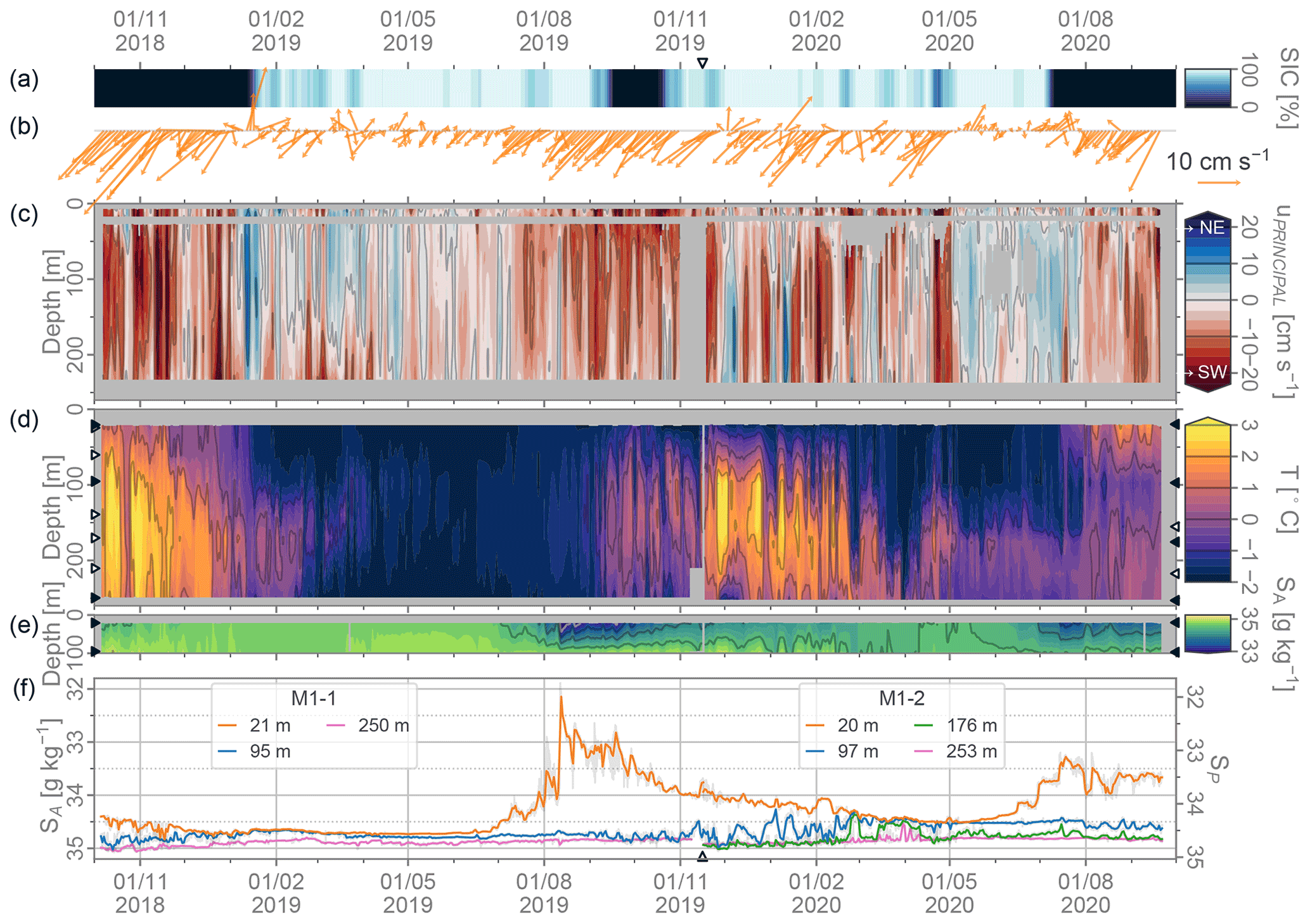
Figure 3The 7 d averaged time series from the M1 mooring. (a) Sea ice concentration at the mooring site from UoB AMSR2, (b) depth-averaged current vector from the RDI150 instrument (29 to 231 m depth), (c) currents along the direction of maximum subtidal variance (positive and blue 45.2∘ CCW of E), (d) in situ temperature, (e) contours of absolute salinity in the upper 100 m, and (f) absolute salinity measured at each individual sensor. In (d) and (e), the mean position of RBR Concerto instruments during the two deployments are indicated with black triangles on either side. The position of RBR Solo instruments (whose vertical position is less certain) is indicated with white triangles.
Very weak northeastward subtidal currents dominated from May until the opening of the sea ice in July (May–July 2020 mean: +0.9 cm s−1), a period in which a thick (>100 m), cold ( ∘C) winter mixed layer overlaid the warmer deep water. Thereafter, the southwestward flow gradually intensified, accompanied by a moderate increase in temperatures through water column, up until the recovery of the mooring in late September. Interestingly, the period of July to September 2020 was the only part of the M1 record where we observed clear evidence of surface warming. As a result, the water column during this period exhibited a mid-depth temperature minimum typical of the remaining “winter water” often found in polar regions, including the northern Barents Sea, during late summer.
3.2.2 Salinity and upper-layer freshening at M1
The salinity records from M1 show strong interannual variability over the study period (Fig. 3e, f). Particularly striking is the upper layer, which was significantly fresher after the melt season of 2019 than before. The near-surface layer was relatively fresh at the start of the record, with SA of 34.4 g kg−1 measured by the sensor at 21 m depth. Salinity was highly variable in autumn 2018 (see Sect. 3.2.5) but generally increased before stabilizing near 34.7 g kg−1 from December until the following summer. The near-surface waters then began to become fresher in the end of June 2019, and SA dropped substantially in the following months, reaching a minimum of <31.9 g kg−1 on 11 August, before the disappearance of sea ice in early September. SA near 20 m depth then increased gradually over the following 7 months, reaching a maximum of ∼34.5 g kg−1 in April 2020. Upper-ocean SA began to slowly decrease again in late May, coinciding with the sea ice melting, before dropping rapidly to a minimum of <33.2 g kg−1 in July and August. The near-surface water remained relatively fresh (SA <34.0 g kg−1 with a few brief exceptions) until the recovery of the mooring in late September 2020.
Deeper in the water column, the record begins with a period of high salinity, with global maxima of SA (>35.05 g kg−1) occurring near 250 m depth in October 2018. These high salinities coincided with the higher temperatures and increased southwestward flow observed during this period (Fig. 3c, d). This relationship between positive anomalies of SA, temperature, and southwestward currents is also present in other parts of the record below 100 m (compare panels c, d, and f of Fig. 3). SA near 250 m decreased gradually between November 2018 and February 2019, before increasing from ∼34.8 to ∼34.9 g kg−1 in early March and remaining on this level through June 2019. Mid-depth salinity increased slightly along with the reappearance of a mid-depth temperature maximum in autumn 2019. During November 2019–January 2020, mid-depth salinity was highly variable and generally covaried with temperature. The highest salinities during the second deployment (SA∼35.0 g kg−1 at 175 m depth) were observed during the temperature peak in November 2019. During spring 2020, mid-depth salinity stabilized at a lower level (∼34.5 g kg−1) than during the preceding year (∼34.8 g kg−1), with some exceptions during the warm anomaly in April 2020.
3.2.3 Comparing M1 and M2
At the M2 mooring, 85 km further east in the northern Barents Sea, the evolution of currents and water masses showed many similarities to that at M1. At both locations, the predominant current direction was towards the southwest (Fig. 4b, c). The axis of maximum current variance within the RDI150 depth range at M2 was oriented along the axis 35.7∘ anticlockwise of east–west, with the mean currents again corresponding approximately to cyclonic flow along the local bathymetric contours. The current records from M1 and M2 are not entirely comparable (the range of the RDI150 ADCP at M2 only extended up to ∼120 m), but it is clear that the depth-average currents at M2 were also strongest in autumn and winter 2018, when a persistent southwestward flow coincided with warmer ocean temperatures (Fig. 4c, d). After this initial period, currents at M1 were generally stronger and more variable on all subtidal timescales. From January 2019, the current record from M2 is dominated by a weak (5–10 cm s−1) flow at depth, and it shows neither the extended periods of strong southwestward flow intensification nor the periods of cessation or reversal observed at M1. The near-surface currents at M2, measured by the upper-ocean ADCP, show a much stronger seasonal cycle, with ice-free periods in autumn corresponding to intensified flow towards the southwest.
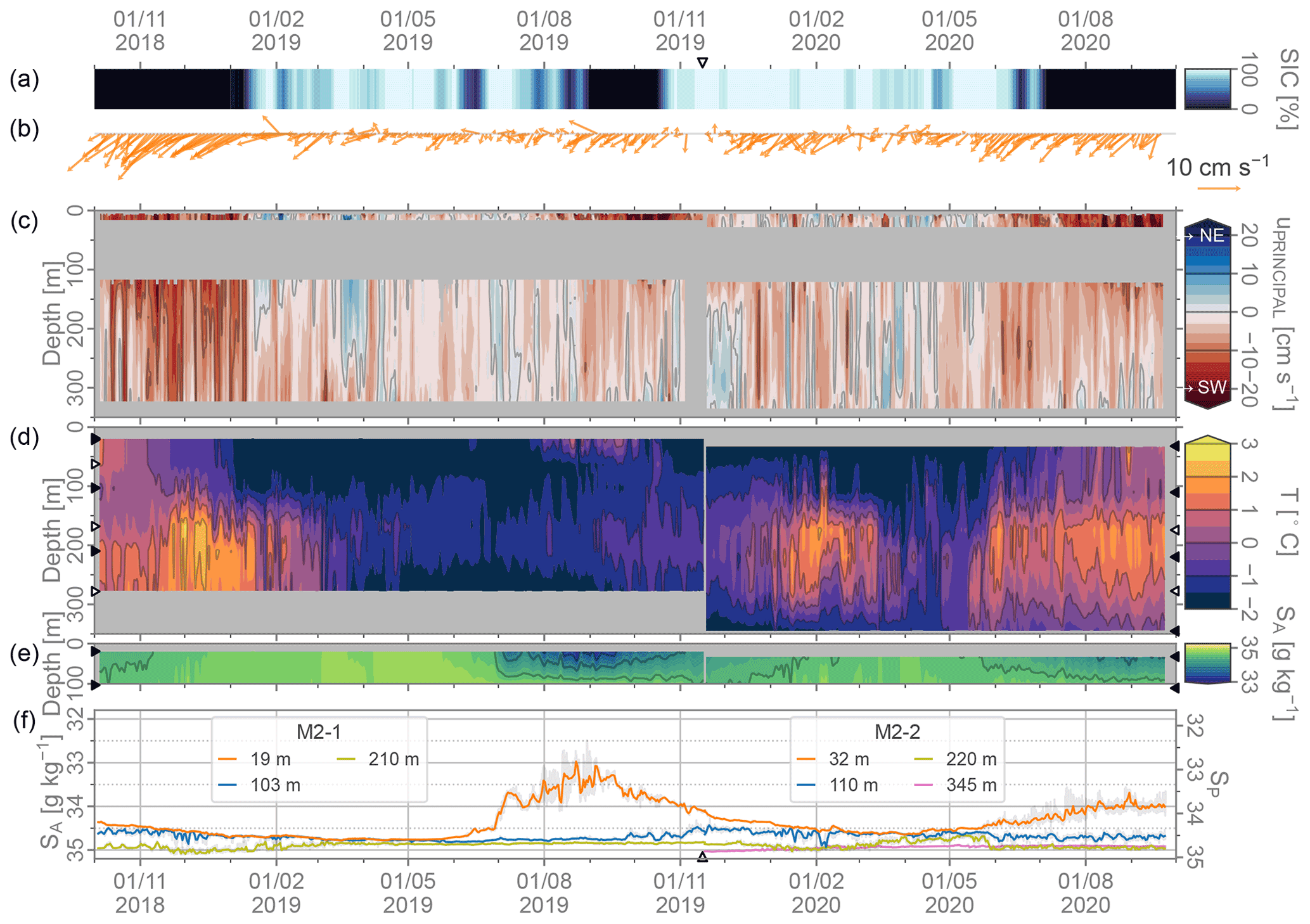
Figure 4(a) The 7 d averaged time series from the M2 mooring. This figure is like Fig. 3, but with a greater y scale, and the depth average current in (b) is calculated between 123 m and 321 m. The direction of maximum subtidal variance (positive/blue in c) is 35.7∘ CCW of E. Note that the uncertainty of the >100 m current direction during the second deployment of M2 is large.
The records from M2, like those from M1, show a mid-depth temperature maximum that weakened and strengthened several times over the study period. Temperature maxima were found somewhat deeper at M2 (∼200 m) than at M1 (∼150 m). The mid-depth temperature maximum at M1 frequently extended into the upper 50 m during warm periods, while warmer waters at M2 were largely restricted to >150 m depth, underlying a cold, uniform layer for most of the study period. A notable difference between the two sites was observed in summer and autumn 2020; a clear temperature maximum (T>1 ∘C) was present at depth at M2 through most of June–September, while temperatures largely remained below 0 ∘C at M1. Temperatures also remained slightly higher at M2 than M1 during spring and summer 2019; a weak mid-depth temperature maximum ( ∘C) remained at M2 during this time. Like at M1, mid-depth salinity at M2 covaried with temperature, with the highest salinities (SA>35 g kg−1 near 200 m depth) occurring during periods of high mid-depth temperature.
Despite the differences outlined above, the overall timing of fluctuations in currents and temperature were similar at the two moorings, although both amplitudes and variability were higher at M1. Figure 5a shows that while mid-depth temperatures were higher at M1 in autumn 2018, temperatures decreased at similar rates at both moorings through winter 2019. Currents (Fig. 5b) also evolved similarly at the two sites in the first year of the joint record, but sub-monthly variability was more pronounced at M1. In autumn 2019, mid-depth temperatures began to rise earlier and more abruptly at M1, with a sudden temperature increase of ∼1.5 ∘C after a period of intensified southward flow, and a second increase of the same magnitude in November, a period of high-amplitude flow variability. During this time, currents remained steadier at M2, and the temperature only increased gradually until the warming rate picked up during December–January. M2 mid-depth temperatures reached a peak (T>1.5 ∘C) around 1 February 2020, after which the temperatures at the two locations again decreased more or less in unison. From April 2020 onward, the temperature and current records diverge between the two moorings, with periods of elevated southwestward flow and increased temperature occurring first at M1 (April–May) and then at M2 (June–September).
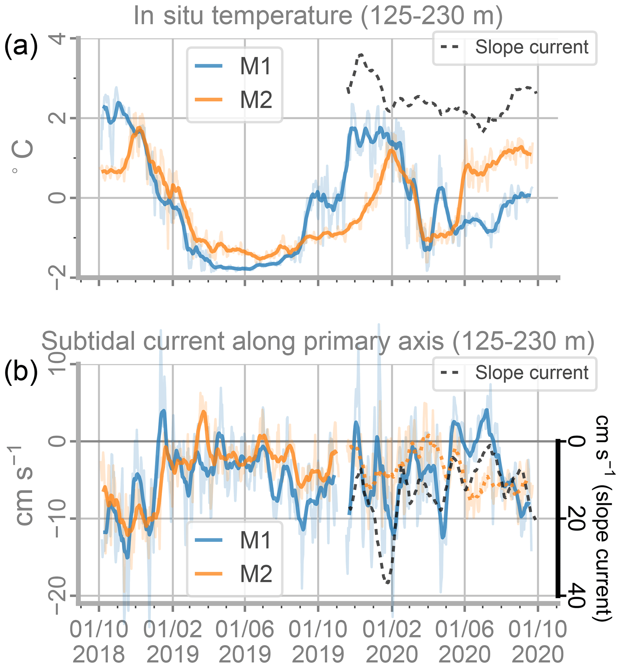
Figure 5Time series from the M1, M2, and AT800 (slope current) moorings of (a) in situ temperature and (b) subtidal currents along the principal axis, both depth-averaged between 125 and 230 m after linear interpolation between available sensors. Thin transparent lines show daily mean quantities, and thick lines show a 15 d running mean (currents from M2–2 are shown as a dotted line to indicate the substantial uncertainty). Note the separate scale for the AT800 slope current in (b).
Also shown in Fig. 5 are temperatures and currents from the AT800 mooring on the shelf slope. The principal axis direction at the AT800 was positive for current direction 49.9∘ CCW of east. The AT800 mooring was located in the FSAW slope current, and generally showed higher temperatures and higher flow speeds than both northern Barents Sea moorings. An episode of intensified flow in January 2020 had no obvious counterpart at M1 or M2, although the southwestward flow at M1 was relatively strong in this period. Temperature increases at AT800 in autumn 2019 and late summer 2020 coincided approximately with periods of increasing temperature at M1.
Upper-ocean salinity evolved similarly at the two northern Barents Sea moorings; strong summer freshening of the near-surface layer occurred at nearly the same time at M1 and M2 both in 2019 and 2020. The clearest difference between the salinity records is that mid-water salinity was lower at M1 than M2 during spring 2020 (compare Figs. 3e and 4e). The apparent downward mixing of fresher water at M1 during this period was not observed at M2. Salinity at the uppermost sensor at M2 remained around 34.5 g kg−1 from February until the subsequent melt season – lower salinity at M1 may indicate that the upper ocean was fresher at M1 than at M2 at this time, but since the sensors were located at depths separated by ∼10 m, a direct comparison is not appropriate.
3.2.4 Water mass distribution
The distribution of Θ and SA at the mid-depth sensors is shown in Fig. 6. Since the sensor depths varied, these distributions cannot be compared directly between moorings and deployments; however, they do provide useful insight into the seasonal water mass variations at mid-depth at the mooring sites.
The distributions are shown along with the water mass classification system for the broader Barents Sea and Nansen Basin region suggested by Sundfjord et al. (2020). We interpret observed water mass distribution in Fig. 6 primarily in terms of two water masses: Atlantic Water (AW, Θ>2 ∘C, SA≥35.06 g kg−1), which originates at lower latitudes and exists on the continental slope north of Svalbard as well as south of the Polar Front, and Polar Water (PW, Θ≤0 ∘C, σ0≤27.97 kg m−3), which is formed in the Arctic Ocean including its shelf seas through cooling and interactions with sea ice and meltwater.
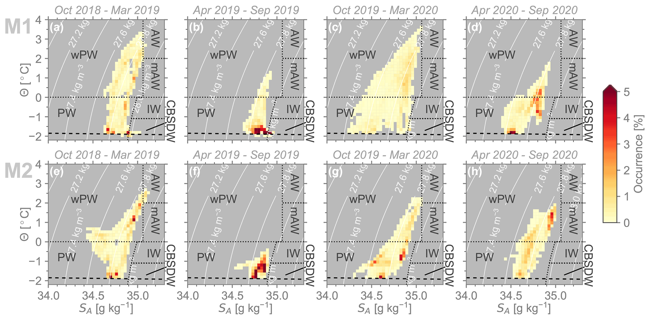
Figure 6Distributions of absolute salinity (SA) and conservative temperature (Θ) in hourly mean data from moored RBR Concerto sensors on the M1 (upper panels) and M2 (lower panels) moorings. Columns show separate 6-month intervals (see panel titles). Only including sensors between 90 and 260 m depth (number and depths of sensors vary; see Table 1). Water mass categories from Sundfjord et al. (2020): AW is Atlantic Water, mAW is Modified Atlantic Water, PW is Polar water, wPW is Warm Polar Water, IW is Intermediate Water, and CBSDW is Cold Barents Sea Dense Water. Dashed black lines show the surface freezing point.
In general, the mid-water Θ–SA distributions at M1 and M2 can be described as a time-varying mixing between these two water masses. However, AW was always modified and almost never present in undiluted form following the strict definitions given above. Throughout the study period, mid-water properties at the moorings largely fell along a trajectory extending from the surface freezing point in the 34.5 to 35.0 g kg−1 SA range, curving upwards and rightwards in Θ−SA space towards the AW classification. Broadly speaking, the transition occurred along isopycnals in the vicinity of σ0=27.8 kg m−3 (with several exceptions detailed below). Along much of this trajectory, water masses fell within the nominal bounds of Warm Polar Water (wPW), which can also originate from solar heating of PW. However, as these movements in Θ−SA-space were largely isopycnal, we interpret them as a signature of mid-water mixing between PW and AW rather than as a result of surface heating – consistent with the measurements being conducted well below the direct influence of surface forcing.
In autumn 2018, the AW influence at M1 was relatively large, with a Θ−SA distribution extending all the way into the AW range (Fig. 6a). Through the following winter, the water became cooler and fresher until the distribution became largely clustered near the freezing line. At the bottom sensor (near 250 m) salinity increased, and in May 2019 Θ−SA properties frequently fell within the range defining Cold Barents Sea Deep Water (CBSDW, ∘C, σ0>27.97 kg m−3), indicating the influence of brine rejection and/or mixing with interior deep waters of the northern Barents Sea. The following periods (Fig. 6c, d) show the reappearance of a weaker AW signal in autumn 2019, followed by a stronger AW signal and a greater spread towards lower salinities as a result of the higher amount of freshwater in the water column (Fig. 3e).
A similar temporal evolution occurred in the Θ−SA distribution at M2, with some notable differences. In the beginning of the record, relatively fresh (∼34.6 g kg−1) and warm (∼0.25 ∘C) water was present near 100 m depth, resulting in a protrusion of the distribution into the fresher wPW range, likely indicating a degree of surface influence (Fig. 6e). The AW core at M2 was also of higher salinity than at M1 during the first months of the record.
The weak mid-depth temperature increase observed at M1 in early autumn 2019 was nearly absent at M2, resulting in a more restricted distribution clustering near SA∼34.8 g kg−1, ∘C (Fig. 6f). The decrease in salinity at M1 in winter 2020 was less pronounced at M2, and for the remaining duration of the study period, the distribution at M2 fell largely along the PW–AW line (Fig. 6g, h).
The Θ–SA distributions from the shallowest sensors, near 20–30 m depth (Fig. 7), reflect the wider salinity range in the upper ocean. During the mostly ice-covered period of April 2019 through March 2020, distributions in the upper ocean were generally clustered close to the freezing line and within the PW water mass boundaries. Some exceptions occurred at M2 due to surface warming in ice-free periods in summer, which resulted in excursions into the wPW range at SA<34 g kg−1. During autumn 2018 and summer 2020, temperature ranges were comparatively wide, and salinity ranges were comparatively narrow. In the upper-ocean sensors, increases in temperature generally occurred along with decreases in salinity, resulting in distributions curving leftward and upward. A notable exception found at M1 during autumn 2018 warrants additional attention.
3.2.5 Episodes of Atlantic Water influence in the upper ocean at M1 during autumn 2018
In general, increases in temperature observed at the uppermost sensors were associated with decreases in salinity (Fig. 7). An exception to this tendency was found in autumn 2018 at M1, where abrupt increases in temperature of up to >1.5 ∘C coincided with increases in salinity of up to >0.3 g kg−1 (Fig. 8). Episodes of concurrent increase in temperature and salinity occurred particularly in late October and November. The two major episodes captured by the upper-ocean sensor at this time occurred during periods of increased southwestward flow throughout the water column (Figs. 3c, 8d). At the peak of both episodes, temperature and salinity at 21 m depth were nearly identical to those at 95 m depth, suggesting that a continuous, very weakly stratified layer extended through much of the water column.
Water properties during these episodes showed a clear tendency upward and rightwards in Θ−SA space (Fig. 8e). This is in clear contrast to upper-ocean warming periods elsewhere in the record (Fig. 7) and suggests that the observed temperature increase in autumn 2018 was due to AW influence rather than heat transfer from the atmosphere. Moreover, atmospheric temperatures measured at the Kongsøya weather station indicate that the atmosphere was significantly colder than the upper ocean during this period.

Figure 7Distributions of absolute salinity (SA) and conservative temperature (Θ) in hourly mean data from moored RBR Concerto sensors on the M1 (upper) and M2 (lower) moorings, only including data from the uppermost Concerto sensors (median depths between 19 and 30 m). See Fig. 6 for details, but note the different scales of the x axes.
3.3 Shipboard CTD transects across flow pathways
CTD transects were conducted across Kvitøya Trough and in the cross-slope direction at the mooring sites within a week-long period in late November 2019 (Fig. 9). All four transects show mid-depth temperature maxima that we interpret as “cores” of AW in various stages of dilution – indicating flow into Kvitøya Trough from the north and cyclonic circulation of AW in the northern Barents Sea consistent with the mooring current measurements. November 2019 was not a period of particularly strong mid-depth temperature maxima at either of the moorings (Figs. 3, 4): at M1, temperatures increased abruptly a few weeks after the CTD transects were made, and at M2, a persistent mid-depth maximum had developed near 200 m, but daily mean temperatures remained below −0.5 ∘C. The 7 d separation between the first and last CTD profile means that the transects cannot be considered as a synoptic “snapshot” of the circulation; however, the transects in combination provide some insight into the distribution and pathways of AW-influenced water in the study area during a time of moderate or weak AW influence.
The northernmost transect (Fig. 9a) shows the southward intrusion of AW into Kvitøya Trough. A broad temperature maximum was found, centred in the western part of the trough near 100 m depth below a ∼25 m deep cold and fresh surface PW layer. In the warm core of the transect near 100 m, temperatures exceeded 4 ∘C and fell clearly within the Θ−SA range of AW.
Further south in the trough, near M1, we observed a thicker (∼50 m) cold surface layer overlying a diluted AW core on the western side (Fig. 9b). The western AW layer extended to the bottom, but a core (∼2 ∘C) was located near 100 m depth. Temperatures decreased rapidly towards the centre of the trough. On the eastern side of the transect, temperatures lay below 0 ∘C throughout the water column.
Cross-slope transects at both mooring sites (Fig. 9d, e) show mid-depth temperature maxima with a warmer core centred over the slope. Both transects also show isopycnals sloping downwards towards the northwest (towards shallower depth), consistent with southwestward geostrophic flow. At the M2 transect, temperatures in the core only reached ∘C degrees, falling entirely within the PW water mass range, but it was clearly distinguished from near-freezing temperatures above and below. At the M1 transect, core temperatures reached >1.7 ∘C, with a Θ−SA signature suggesting some mixing with AW and large fluctuations in the profiles indicating interleaving of water masses on the top of the core near 100 m depth.
3.4 Correlation between ocean currents and atmospheric forcing
Ocean currents displayed high subtidal variability on intraseasonal timescales (a few days to approximately one month) at both moorings but particularly at M1 (Sect. 3.2). Especially in autumn, there were frequent episodes of abrupt intensification and slowdown of the currents and occasionally even reversal of the flow direction. These fluctuations also exerted a strong influence on the hydrography at shorter timescales, as shown by the covariability of currents and temperature in Figs. 3 and 8. Atmospheric pressure was also quite variable on sub-monthly timescales (Fig. 2b), related to the passage of weather systems. We investigated the relationship between synoptic atmospheric variability and ocean currents during the study period in order to determine whether the observed ocean flow variability at the moorings was driven by the atmosphere.
Figure 10a–h show the correlations between the eastward and northward vector components of daily CARRA 10 m winds and ocean currents at the moorings at M1 (upper row) and M2 (middle row). Ocean currents are in this case taken as the along-axis subtidal currents, positive towards the NE, and depth-averaged between 125 to 230 m (shorthand ). Correlations were evaluated with time lags of ±7 d after the 61 d running mean was subtracted from both time series in order to focus on the relevant timescale. The r values shown in Fig. 10 show maximum amplitude correlations alongside the lag in days at which maximum correlation is attained.
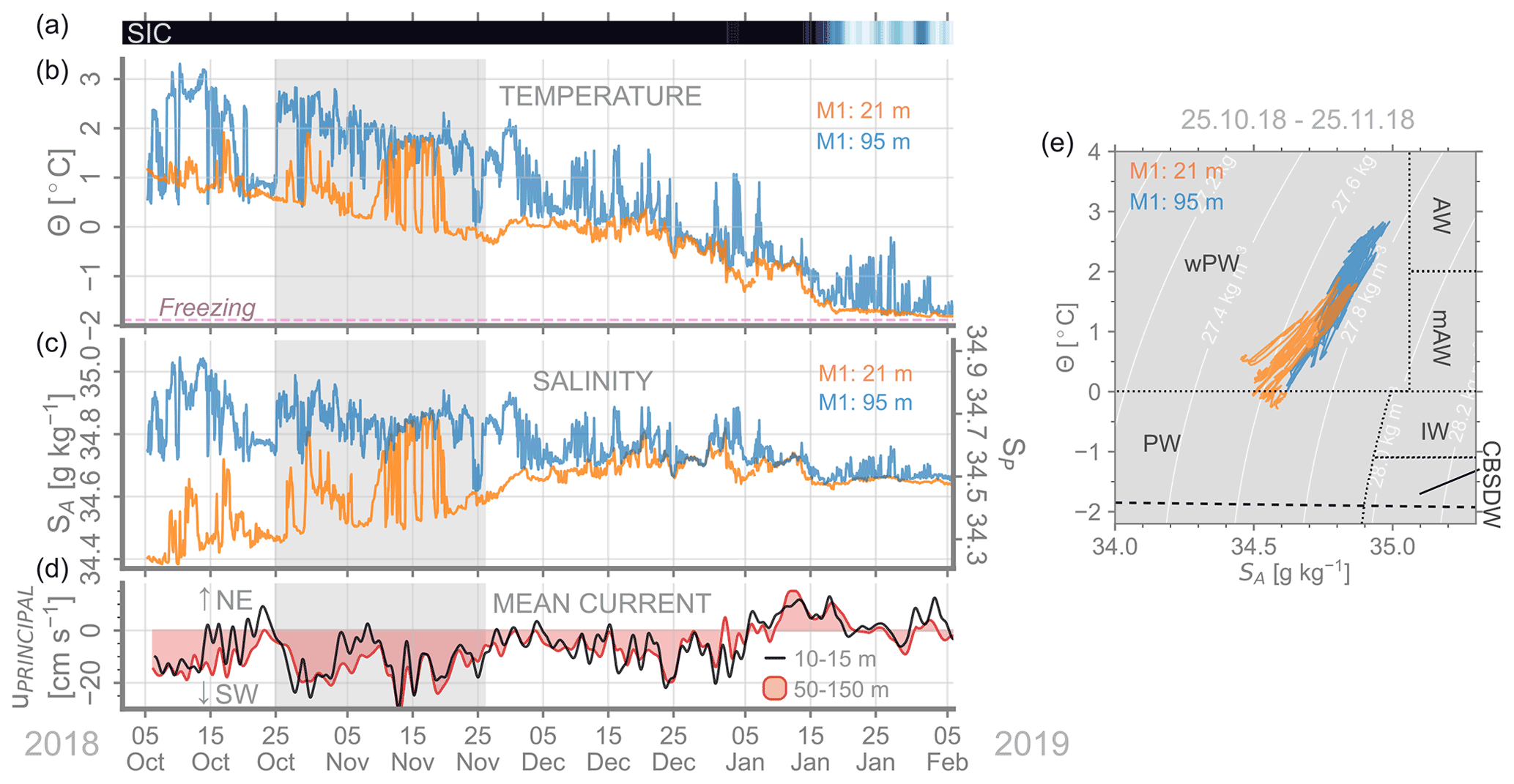
Figure 8Upper-ocean state at M1 during autumn 2018 to winter 2019. (a) Local sea ice concentration (colour scale as in Figs. 3a, 4a). (b) Hourly mean conservative temperature from the M1 mooring at 21 m (orange) and 95 m (blue) depth. The dashed pink line shows the freezing temperature at SA=34.65 g kg−1. (c) Absolute salinity from M1 at 21 and 95 m depth. (d) Mean subtidal currents at 10–15 m depth (black, from Sig500 instrument) and 50–150 m depth (red, from RDI150 instrument), both filtered as described in Sect. 2.1.4. (e) Hourly data from the 21 m (orange) and 95 m (blue) sensors in Θ−SA space. Only showing data from the period 25 October through 25 November, highlighted in grey in panels b–d.
The strongest correlations were found between zonal winds and at M1 (Fig. 10a): negative correlations, indicating that intensified northeastward ocean currents were associated with westward wind anomalies and vice versa, were found over a large region encompassing the ocean around Svalbard, with the strongest correlations () in the northwestern Barents Sea. Over most of this area, the lag maximizing the correlation (Fig. 10b) suggests that the regional winds led the ocean currents at M1 by 2 d. The much weaker correlation with northward winds (Fig. 10c) suggests that it was mainly the zonal wind forcing that was correlated with the ocean variability at M1. Ocean currents at M2 were also more strongly correlated with zonal than meridional winds. In general, however, correlations between currents and winds were weaker at M2 than at M1. Time lags between zonal wind forcing and currents maximizing correlation at M2 were 2–3 d.
On the timescale in question, variability in the wind field is dominated by the passage of weather systems. The correlations above suggest that the currents were related to zonal wind forcing (especially at M1), which in turn is associated with a meridional atmospheric pressure gradient. For the following analysis, we found it useful to define an index ΔPK−B based on observational time series from two automatic weather stations spanning 625 km of meridional distance:
where PKVITØYA and PBJØRNØYA are the daily mean atmospheric pressure measured at weather stations on Kvitøya and Bjørnøya, respectively (see Fig. 1). This definition was not chosen in order to maximize correlations but to provide a simple, observationally based index of the atmospheric state affecting wind forcing in the northern Barents Sea area: positive ΔPK−B corresponds to lower pressure toward the south, while negative ΔPK−B corresponds to lower pressure toward the north. As expected from geostrophy, positive ΔPK−B generally corresponds to westward surface winds in the area between the two weather stations, and negative ΔPK−B generally corresponds with eastward winds. This is confirmed by the correlation between ΔPK−B and 10 m wind components in CARRA (Fig. 10i–l): ΔPK−B is strongly negatively correlated at zero lag with the eastward wind component over the entire northern Barents Sea and the AW inflow region of the Nansen Basin. Although maximum amplitude correlations were attained between the two weather stations, it is clear from Fig. 10i that zonal wind variability over a large area around Svalbard can be explained by the north–south pressure gradient captured by ΔPK−B.
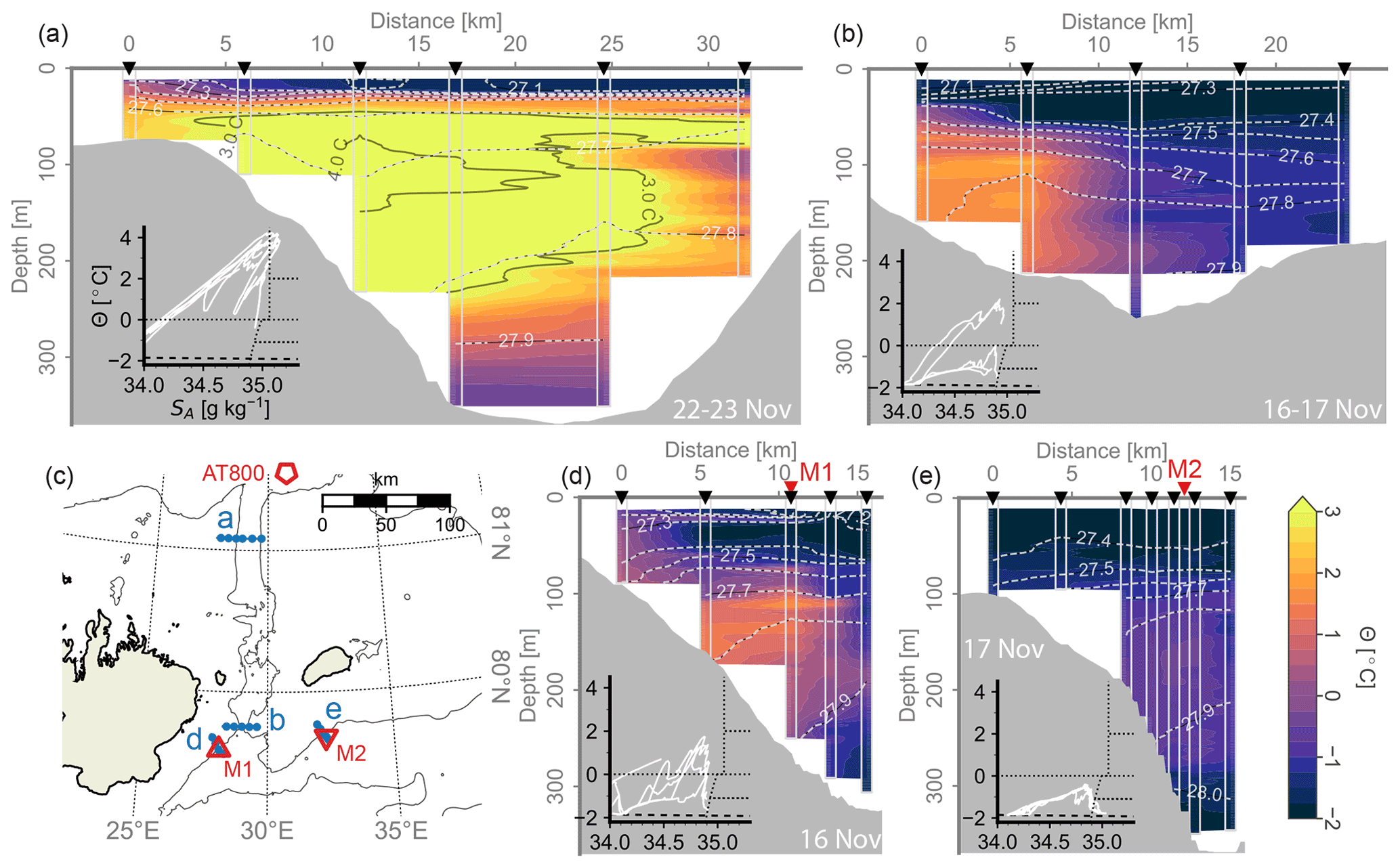
Figure 9Shipboard CTD transects in November 2019. (a, b, d, e) Contours of conservative temperature (coloured contours, grey contours above 3 ∘C) and σ0 (kg m−3, labelled dashed white or grey line contours). Small inset plots show the transect CTD profiles in Θ,SA space (white lines); see Fig. 6 for water mass categories indicated in dashed lines. (c) The location of the transects (blue), plotted along with the 250 m contour (grey) and the mooring locations (red). Transect dates are shown in each panel.
Having established that ΔPK−B is a useful index of the overall atmospheric forcing, we went on to examine the relationship between this index and the ocean currents measured at the moorings. Figure 11 shows a comparison between mean subtidal mid-depth currents at the two moorings and the ΔPK−B index. Through much of the study period, there was a clear relationship between ΔPK−B and currents at M1, with negative ΔPK−B associated with southwestward current anomalies and vice versa. We evaluated the relationship quantitatively by computing correlations between daily time series of (i) ΔPK−B and (ii) along-axis subtidal currents , after removing the 61 d running mean from both time series in order to focus on the relevant timescale. Correlations were evaluated for all three moorings with lags (atmosphere leading the ocean) spanning between 0 and 7 d and are shown in Table 3. The resulting maximum correlation between ΔPK−B and at M1 was r=0.47 at a lag of 2 d, confirming a moderate positive correlation between the variables at M1. At M2, the maximum lagged correlation, also at a lag of 2 d, was positive but weak, and at AT800 it was negative but weak.
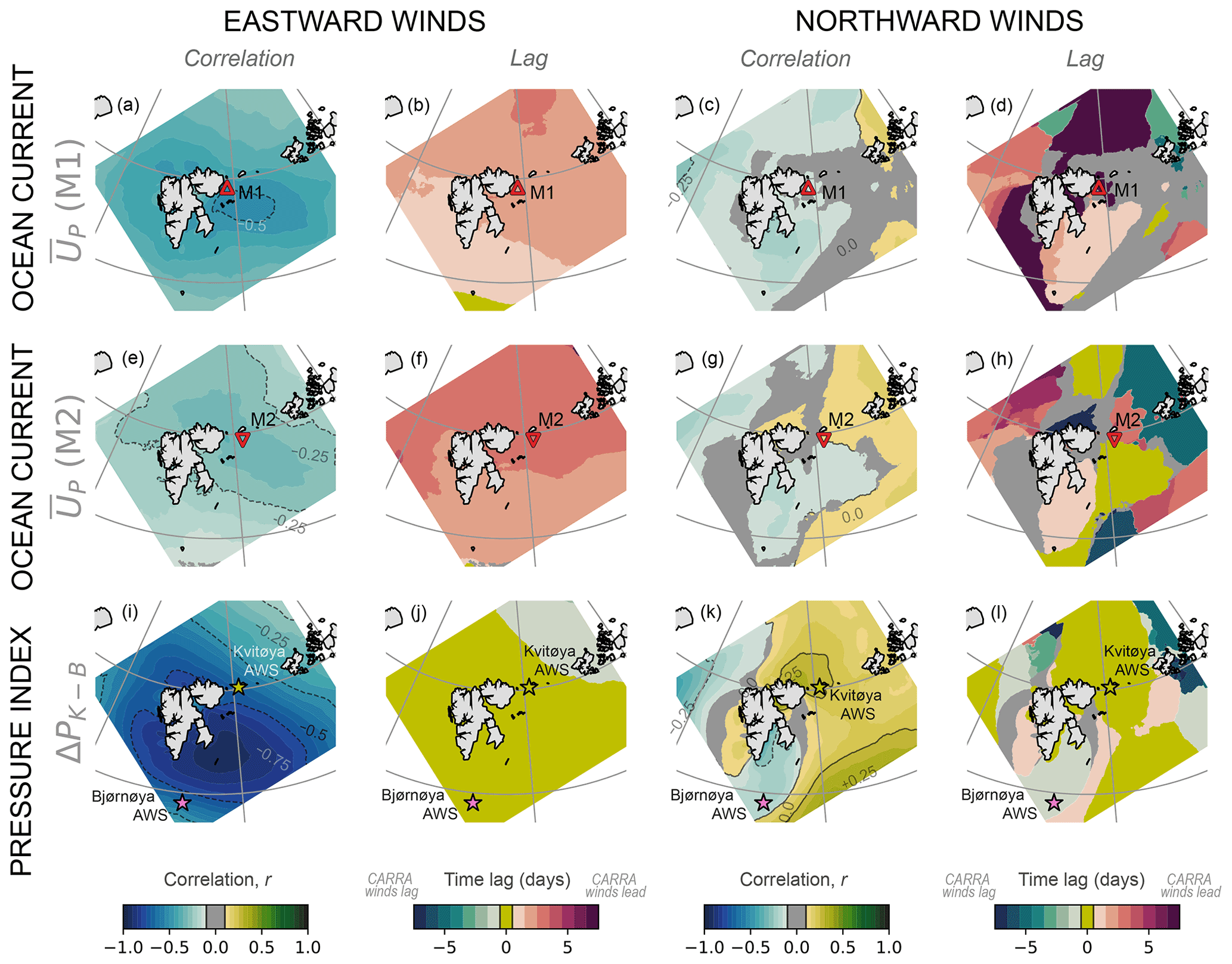
Figure 10Correlations between CARRA 10 m winds and ocean currents , positive towards the ∼NE, at M1 (upper) and M2 (middle), and the ΔPK−B pressure difference, positive for lower pressure at Bjørnøya (bottom). Panels on the left side (a, e, i) show the maximum correlation with the zonal eastward wind vector component, and the time lag at which the maximum correlation is attained (b, f, j). Green (red) colours mean that the CARRA winds lag (lead) the correlated variable. The right side shows the maximum correlation (c, g, k) and time lag (d, h, l) with the meridional northward wind vector component. Correlations are computed for the available time series between 1 October 2018 and 1 October 2020, using a spatial subset of the CARRA-East domain. Grey areas indicate where no significant correlation 0.1 was found at any lag. All time series are daily means that have been high-pass-filtered by removing the 61 d running average before computing correlations.
Table 3Correlation between ΔPK−B and (positive towards the ∼NE) shown in Fig. 11. The 61 d running mean has been removed from both time series. Showing the maximum lagged correlation, with the time lag (ΔPK−B leading ) maximizing the correlation in parentheses. Calculated for the full available time series within 1 October 2018–1 October 2020, excluding “heavy sea ice periods” and only including “heavy sea ice” periods. Non-significant (p<0.05) correlation values shown in italics.
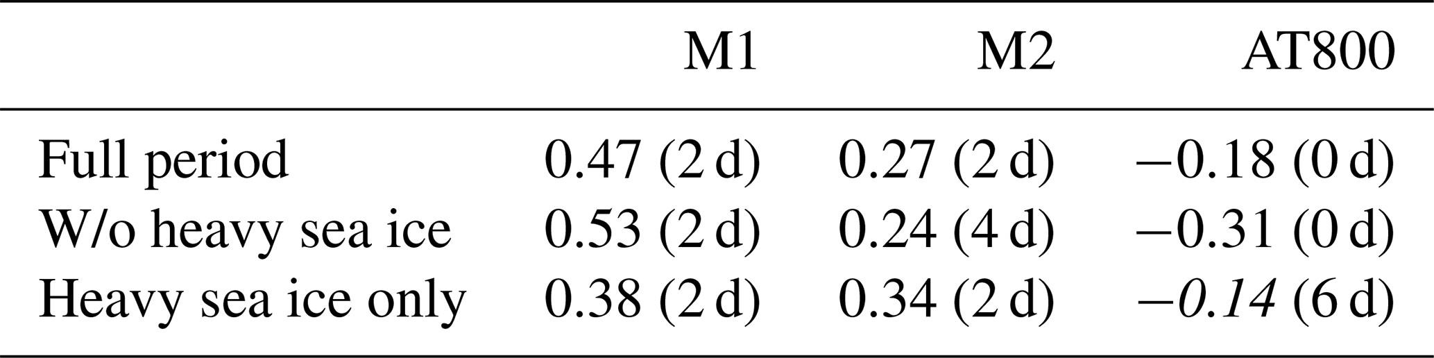
We recomputed correlations after removing parts of the record where sea ice concentration was consistently high in the northern Barents Sea. Two time periods, March–June 2019 and December 2019–March 2020, were defined as heavy sea ice periods (Fig. 11a, d). The correlation at M1 increased slightly when heavy sea ice periods were excluded and decreased when calculating the correlation within the heavy sea ice periods (Table 3). At M2, the maximum correlations were higher during the heavy sea ice periods than in the remaining time series. At AT800, a significant correlation was not found when only including the heavy ice period.
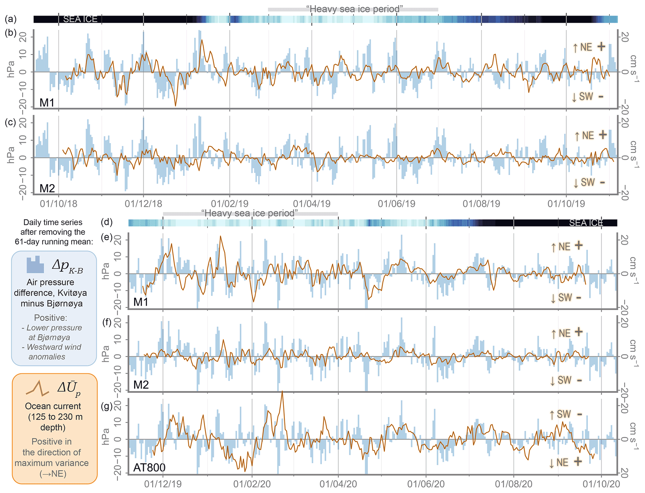
Figure 11Unlagged time series of daily mean ocean currents, surface air pressure gradient, and sea ice concentration, after removing the 61 d running mean. (a, d) Northern Barents Sea sea ice concentration (average in the A-nBS area, with the same colour scale as in Figs. 3a, 4a). All remaining panels show ΔPK−B, the pressure differential between Kvitøya–Bjørnøya (blue), and 125 to 230 m depth-averaged ocean currents in the principal direction (positive ) from ADCPs at different moorings (black/orange). (b, e) Currents from M1, positive 45.2∘ CCW of east. (c, f) Currents from M2, positive 35.7∘ CCW of east. (g) Currents from AT800, positive 49.9∘ CCW of east (note that the scale of the y axis has been reversed).
Cross-spectral analysis of the time series of ΔPK−B and at M1 show significant coherence at a range of frequencies, with notable peaks in coherence squared near periods of 3.5, 11, and 18 d (Fig. A1 in the Appendix). A lag of ∼2 d was typical across a wide range of frequencies (Fig. A1d), broadly consistent with the lagged correlation analysis.
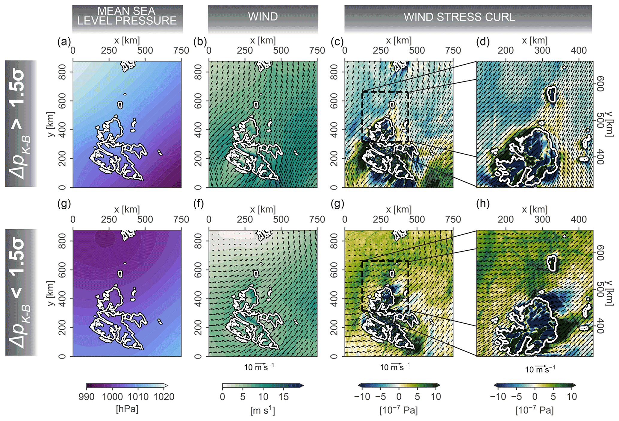
Figure 12Atmospheric variables in a regional subset of CARRA-EAST during the period 2018–2020, showing the average of daily mean conditions on days where ΔPK−B (after subtracting the 61 d daily mean) exceeds 1.5 standard deviations above (upper) and below (lower) its average. (a, g) Average mean sea level pressure. (b, f) Average wind at 10 m. The green contour indicates the magnitude of the average wind vectors. (c, g) Average wind stress curl with average wind vectors. Panels (d) and (h) are like (c) and (g) but are zoomed in on a smaller region around Nordaustlandet and Kvitøya. Axis coordinates show the grid coordinates, which are equally spaced at 2.5 km resolution. Wind vectors (black) are subsampled every 15th grid point in (b), (c), (f), and (g) and every 5th grid point in (d) and (h).
We also evaluated the correlations between ΔPK−B and at M1, respectively, and the daily average wind stress curl computed from CARRA. Correlations were evaluated with time lags of ±7 d. The results indicate that both variables are weakly correlated with negative wind stress curl over Kvitøya trough and over the FSAW core north of Svalbard (Fig. A2). Correlations with wind stress curl were generally maximized at a lag of 1–4 d for , and at zero lag for ΔPK−B. Looking more closely at the state of the atmosphere during negative and positive pressure meridional differences, Fig. 12 shows the regional patterns of sea level pressure, wind, and wind stress curl during periods in 2018–2020 where ΔPK−B exceeded 1.5 standard deviations above or below its mean value (after subtracting the 61 d running mean). High ΔPK−B, corresponding to lower pressure to the south and decreased ocean inflow at M1, was associated with easterly winds and negative wind stress curl in offshore areas north of Svalbard and in most of the Barents Sea. Conversely, periods of low ΔPK−B, corresponding to higher pressure to the south and stronger ocean inflow into the northern Barents Sea, show a pattern of westerly winds and positive wind stress curl in these same areas. During both phases, these patterns were often quite different close to the coasts as winds interact with the land mass. Notably, the mean wind stress curl during high ΔPK−B changed sign from negative to positive toward the coast north of Svalbard (Fig. 12d). During low ΔPK−B, the study area encompassing M1 was found on the lee side of Nordaustlandet in the vicinity of strong coastal wind stress anomalies of opposite sign to the north and south (Fig. 12h).
4.1 Seasonal evolution of the water column
As might be expected, the records from the M1 and M2 moorings show that the upper ocean in the northern Barents Sea is strongly influenced by the presence of sea ice. Strong freshening occurs during the melt season, and warming of the surface layer occurs during ice-free periods in summer, when heat can be transferred directly from the atmosphere to the surface ocean. Interestingly, the onset of the drop in salinity near 20 m depth occurred 1–2 months before the decrease in sea ice concentration, likely as a result of a combination of local ice melting and thinning and advection of meltwater from regions nearer the ice edge. During both 2019 and 2020, surface freshening occurred earlier at M2 than at M1. This can be explained as a result of the progression of sea ice melting in the northern Barents Sea, which during both seasons advanced from east to west.
The upper ocean preserves a lasting impact of the preceding sea ice season. Salinity at 20 m depth at M1 was 0.5 to 1.0 g kg−1 higher in autumn 2018 (following a long ice-free summer) than in autumn 2019 (following a summer of persisting ice cover in the western northern Barents Sea). The year-to-year difference is in qualitative agreement with Aaboe et al. (2021), who estimated a 1 m increase in freshwater content in the northern Barents Sea from 2018 to 2019. Interannual variations in wind forcing influences sea ice drift between the Arctic Ocean and the Barents Sea (Sorteberg and Kvingedal, 2006), and the high sea ice year of 2019 in the northern Barents Sea was a result of large sea ice imports from the north and, to a lesser degree, east, during winter 2018/2019 (Aaboe et al., 2021). The ice ultimately melted in the Barents Sea, supplying freshwater to the surface ocean during the melt season. Lind et al. (2018) showed that increased upper-ocean freshening and strengthened salinity stratification as a result of strong sea ice imports reduces vertical mixing with deeper waters and preconditions the region for further sea ice growth the next winter. Based on our data, it is certainly conceivable that the absence of strong freshwater stratification in autumn 2018 was in part responsible for the late onset of the sea ice in the northern Barents Sea this season (January 2019) compared to the following season (October 2020). However, the return of a thick and extensive sea ice cover (Aaboe et al., 2021) and a fresh upper-ocean layer in 2019 suggests that a sufficiently large import of sea ice can return the northern Barents Sea to a cold, stratified, and ice-covered state. Further investigation of the relationship between salinity stratification and preceding sea ice season would greatly benefit from observations with higher vertical resolution than the single-depth sensors in this study provide. In particular, time series observations of mixed-layer depth and integrated heat and freshwater content throughout the melt season and freezing season should allow a more quantitative investigation of the air–ice–sea interplay.
Interannual differences in salinity were not restricted to the upper ocean; at both moorings, the mid-depth waters were also fresher during spring 2020 than during spring 2019. While this could in part be related to varying rates of AW inflow during these 2 years, we mainly attribute it to different rates of meltwater being mixed down from the surface fresh layer and the sustained effect of meltwater inputs over 1 to several years. This is particularly the case at M1, where the 34.5 g kg−1 isohaline frequently extended to ∼100 m depth during winter and spring 2020. The fresher water at mid-depth at M1 compared to M2 may be explained by ocean advection through the Kvitøya–Nordaustlandet gap. While the northern Barents Sea was largely ice covered during early 2020, sea ice concentration north of Nordaustlandet and in the Kvitøya Trough area was more variable. In these partially ice-free areas, mid-depth water masses influenced by increased wind-driven vertical mixing may have been advected southward to M1 along with the prevailing ocean currents. This is supported by the relatively strong southwestward flow observed at M1 (and largely absent at M2) during this period – including episodes of intensified southwestward currents coinciding with intermittent decreases in temperature and salinity down to 175 m depth.
The water masses observed at the moorings at mid-depth and below can generally be described as Polar Water mixed with varying amounts of Atlantic Water. In addition to the freshwater influence described above, notable exceptions to this include (i) the relatively fresh and warm waters observed above 100 m M2 in October–November 2018 and (ii) the cold, saline deep waters found near 250 m depth at M1 in spring 2019. We associate the first with downward mixing of fresher water masses that had been heated at the surface in summer. The second we interpret as the influence of brine rejection and cooling during sea ice formation. It is not clear whether these saline deep waters, which were close to surface freezing temperature, were produced locally or transported from other areas. The high sea ice concentration at the M1 mooring location at the time may suggest the latter, as there appears to have been few areas of open water locally where freezing could occur. This is in line with previous studies showing that dense water is formed extensively on the banks and ends up filling the bottom of the deep trenches of the northern Barents Sea (Midttun, 1985; Årthun et al., 2011). However, it is possible that dense water formation occurred shoreward of M1, in small coastal polynyas or other nearby shallow areas.
The signature of Atlantic Water is recognizable as a mid-depth temperature maximum, varying in strength through the study period. At M1, the maximum was typically found between 100 and 200 m depth during periods of strong AW influence, while it was located below 150 m at M2. The vertical extent of the AW signal at M1 varied from spanning most of the water column in autumn 2018, disappearing gradually in winter, reappearing as a more localized maximum around ∼150 m depth in autumn 2019, and finally persisting as a weak warm layer below 150 m depth through most of 2020. The latter is the vertical structure typically observed in the northern Barents Sea (e.g. Loeng, 1991; Lind et al., 2016).
The AW layer observed at the mooring sites was generally situated below a colder and less dense layer extending to the surface. This upper layer will have constituted a stratification barrier between the AW below and the ocean surface above, reducing vertical mixing and preventing the transfer of heat from the AW layer and the upper ocean, sea ice, and lower atmosphere. The near-surface waters varied in temperature depending on surface forcing, but they were distinguishable from the AW layer by their lower salinity. However, an interesting exception was observed at the M1 mooring during autumn 2018, when temperature and salinity near 20 m depth increased during episodes of strong inflow from the north, consistent with the influence of AW in the uppermost part of the water column. Weak freshwater inputs during the unusually long 2018 ice-free season may have resulted in a weak stratification that allowed AW to extend through the water column and the upper-ocean temperature front to progress southward into the northern Barents Sea. This finding is in line with Lind et al. (2018) in indicating that sea ice melt plays a key role in regulating the vertical extent of the AW layer. Given the lack of freshwater inputs and relatively vigorous wind forcing in autumn, it is likely that the AW influence extended to the ocean surface during these inflow periods. Since the air was substantially colder than the ocean, it is likely that the presence of warm AW-influenced waters at the surface resulted in increased transfer of heat from the ocean to the lower atmosphere. It may also have contributed to maintaining the ocean's ice-free status well into winter, until the massive sea ice inflows from the north began in January 2019 (Aaboe et al., 2021).
Compared to the AW-dominated ocean south of the Polar Front, the northern Barents Sea can be described as a cold, stratified, PW-dominated ocean environment (e.g. Loeng, 1991; Ingvaldsen et al., 2021). Our findings suggest that there are important local caveats to this general picture, as they show the strong influence of AW over large parts of the water column in inflow regions of the northern Barents Sea during late autumn and winter. The observed seasonal hydrographic variability was to a large degree driven by inflows from the north, highlighting the strong influence that ocean advection exerts on the physical environment. The northern Barents Sea experiences strong seasonality in general, and the seasonal timing of the AW inflow generally coincides with cooling of the atmosphere and an increase in sea ice concentration. Hydrographic surveys in the region have largely been based on shipboard measurements in late summer or early autumn – the mooring records presented in this study show the need for observations collected during different times of the year in order to accurately describe and monitor the ocean environment.
4.2 Circulation of Atlantic Water in the northern Barents Sea
The observed prevailing southwestward current direction at the two moorings is consistent with a topographically steered, cyclonic ocean circulation in the northern Barents Sea. At both moorings, increases in southwestward flow coincided with increased mid-depth temperatures. This implies that some of the AW that is transported along with the FSAW north of Svalbard leaves the eastward path of the main current and enters the northern Barents Sea at its northern boundary.
Cross-slope CTD transects collected in November 2019 indicate that the flow is concentrated over the bathymetric slope. This is typical of ocean circulation at high latitudes, where weak stratification and strong rotational influence combine to vertically interlock the water column and steer flow along bathymetric contours. Surface forcing of the ocean over contours of constant potential vorticity favours cyclonic flow (Nøst et al., 2008), consistent with the predominant anticlockwise AW circulation in the Arctic Ocean and the Nordic Seas (Aagaard, 1989; Jones, 2001) and the currents observed in the northern Barents Sea in this study.
The southward transport of AW into troughs north of the Barents Sea has previously been indicated by model studies and hydrographic measurements within the troughs (Aksenov et al., 2010; Pérez-Hernández et al., 2017; Menze et al., 2020). The two moorings in this study were positioned downstream of two troughs connecting the northern Barents Sea with the FSAW, Kvitøya Trough, and Franz Victoria Trough. The latter trough is far wider and deeper than the former, but our findings suggest that transport through Kvitøya Trough has a profound influence on the hydrography in the study region north of Kong Karls Land.
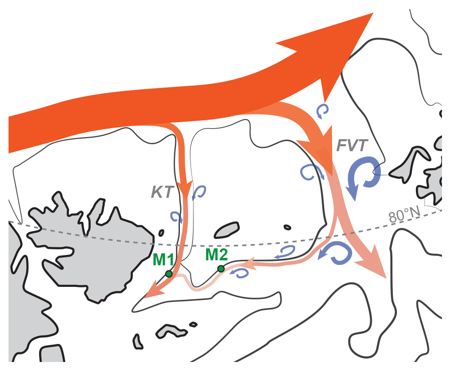
Figure 13Conceptual interpretation of the advection of Atlantic Water into the study area during the inflow phase in late autumn and early winter. Orange arrows represent AW that is cooled and diluted along the pathways into the northern Barents Sea. Blue arrows represent modification through lateral mixing with ambient water masses and surface cooling and freshening. Black lines represent the ∼250 m depth contour.
We interpret our findings as follows: AW-influenced water masses enter the northern Barents Sea through both Kvitøya Trough and Franz Victoria Trough, with the core of the inflow concentrated over the topographic slope (Fig. 13). Kvitøya Trough constitutes the more direct route, and the AW arriving through this pathway tends to be warmer and less diluted. The water flowing through the broader Franz Victoria Trough and entering the study area from the east follows a longer trajectory after leaving the FSAW, and it is therefore subject to more surface influence and more mixing with Polar Water before arriving south of Kvitøya.
The following observations from this study support this interpretation.
-
The AW signal was more pronounced at M1 than at M2 during most of the study period, maximum temperatures were higher, and the vertical extent of the warm core was greater, in line with it being closer to the source in the FSAW.
-
Shipboard CTD transects from November 2019 suggest a continuous core of AW-influenced mid-depth waters extending from the northern opening of Kvitøya Trough to the M1 mooring. The signal was strongly diluted through the trough but remained clearly recognizable as a localized core at M1. An AW-influenced core was also present at M2 during the same period, but there it was significantly more diluted and somewhat deeper.
-
AW arrived at the two mooring sites at different times. In particular, the seasonal inflow of AW at M1 seems to precede that at M2 by 1 to 2 months, consistent with changes in the FSAW taking longer to propagate through Franz Victoria Trough than Kvitøya Trough. The distance to M1 along the 250 m contour from the intersection of the FSAW with the opening of Kvitøya Trough is on the order of 200 km. From the same point following the contour eastward to Franz Victoria Trough, southward into the northern Barents Sea, and westward to M2, the distance is close to 450 km. Advection along the differential distance of 250 km over 1 to 2 months would imply a mean speed of 5 to 10 cm s−1, a figure that seems reasonable given the observed currents.
-
While AW-influenced water was frequently found above 100 m depth at M1, it was generally located below a colder, ∼150 m deep surface layer at M2. The longer pathway through Franz Victoria Trough means that water masses arriving at M2 have been subject to more surface cooling and mixing with cold and fresh upper-ocean water masses in the northeastern BS.
-
Flow and water mass characteristics were generally more variable at M1. The inflow at M2 appeared more sluggish, with less frequent intermittent intensifications and reversals of the flow. This suggests that the flow through Kvitøya Trough is relatively responsive to forcing. The flow along the longer pathway through Franz Victoria Trough, where the forcing is integrated over a longer time and a greater area, may effectively filter out upstream variability on shorter timescales by the time it arrives at M2.
It should be noted that since we do not have ocean observations to the east of M2, we cannot conclusively state that the eastern pathway indicated in Fig. 13 is the origin of the warm water that arrived at this mooring. For example, some AW could also penetrate through the topographic depression extending southwestward on the eastern side of Kvitøya (Fig. 1), which forms a continuous pathway from M2 to the northern slope above ∼170 m depth. However, since the AW maximum at M2 was typically located near 200 m depth, and the cross-slope CTD transect at M2 indicated an AW core situated deeper than the 200 m isobath, we consider it likely that the pathway indicated in Fig. 13 is the main one.
Heat transport in the FSAW undergoes a seasonal cycle associated with the eastward propagation of the seasonal cycle of AW from Fram Strait (Ivanov et al., 2009; Lique and Steele, 2012). The observed seasonal cycle in the hydrography at M1, with the arrival of AW in autumn, is consistent with previous mooring observations from the continental slope north of Svalbard (Renner et al., 2018; Lundesgaard et al., 2021) and supported at least qualitatively by the temperature evolution observed in the core of the FSAW north of Svalbard in 2019–2020. The seasonal cycle in the FSAW has a first-order impact on the evolution of the water column at the M1 and M2 moorings. This underscores that advection from the north is a key driver of the ocean environment in the northern Barents Sea.
The seasonal cycle in the FSAW affects the current strength and the water properties; the phase of maximum temperature is also associated with a maximum of eastward volume transport (Renner et al., 2018; Pérez-Hernández et al., 2019). This was also the case at M1 and M2 during the study period; the southwestward flow and the temperature peaked during late autumn to early winter. It seems likely that the magnitude of the advection into the northern Barents Sea is coupled to the strength of the FSAW over seasonal timescales, with increased eastward flow along the northern shelf slope resulting in increased transport through the troughs to the south. The dynamics governing the interactions between slope currents and submarine troughs are complex and may involve non-linear dynamics and instabilities of the along-slope flow (Dinniman and Klinck, 2004; Jordi et al., 2008; Nilsen et al., 2016). Since both the southward advection and the upstream heat content undergo seasonal cycles with similar phase, both are likely to contribute to the seasonality in heat transport into the northern Barents Sea.
Our findings document the entry of diluted AW into the northern Barents Sea from the north, but they say little about the downstream pathways of the imported waters. The 250 m depth contour continues southwestward from the M1 mooring, but then turns sharply towards the east as the seafloor rises abruptly toward the small archipelago of Kong Karls Land. If the current core remains strongly constrained to constant depth, the flow might be expected to turn eastward and enter the eastern parts of the northern Barents Sea, where it might eventually mix with the ambient waters or continue to circulate clockwise around Kong Karls Land. The bathymetric constraints are not absolute, however, and non-linear dynamics may come in to play, particularly near the sharp wedge in the bathymetry downstream of M1. Here, the small length scales may result in a large Rossby number, favouring ageostrophic flow (e.g. Phillips, 1963). Isobaths also diverge in this area, perhaps resulting in a slowing down of the currents and a widening of the current core. Nilsen et al. (2016) argued that at large Rossby numbers, the slope current core will tend to deflect towards shallower depth in regions where the slope becomes less steep. Moreover, vorticity forcing associated with nearshore gradients in wind stress forcing may also act to bring some deeper water up onto the shelf. It is therefore not unlikely that some of the diluted AW observed at M1 may penetrate southward and onto the shelf west of Kong Karls Land.
The 2-year record is too short to confidently distinguish between interannual and seasonal variations. However, it is interesting to observe that during 2018–2020, the onset of southwestward flow and mid-depth temperature increase occurred out of phase with the warming of the atmosphere. As such, the area seems to experience successive maxima in incoming radiation (June), air temperature (mid to late summer), and warming of the ocean below the mixed layer (late autumn to early winter). A seasonal pulse of warm mid-ocean waters in autumn and winter may be a consistent feature of the ocean environment in the northern Barents Sea. Occasionally, the seasonal pulse takes place below the sea ice cover, such as in 2019. The AW inflow branches frequently carry nutrients (Torres-Valdés et al., 2013) and marine organisms native to lower latitudes (Wassmann et al., 2015) into the Arctic – it is unclear what role a seasonal AW pulse from the north into the dark and often sea-ice-covered northern Barents Sea may play for the regional marine ecosystem.
As a note of caution, the mooring records shown in this study allow us to make qualified inferences about the circulation, but they are each restricted to a single location within inflow current cores. This study does not provide a comprehensive view of the regional circulation, nor does it attempt to quantify the advective fluxes of water, heat, and salt. At the time of writing, additional ocean moorings are in place across the slope at M1 – these will hopefully help estimate the transports associated with the flow and to study the dynamics of the slope current in more detail.
4.3 Atmospheric modulation of inflow from the north
Our findings demonstrate a correlation between the meridional atmospheric pressure gradient and the southwestward flow at depth at the M1 mooring (and to a lesser degree at M2). Low air pressure at Bjørnøya relative to Kvitøya, corresponding to cyclonic, westward wind anomalies in the northern Barents Sea and the AW inflow region north of Svalbard, tend to coincide with a reduction of the southwestward ocean current and vice versa. The atmospheric forcing leads the ocean response by approximately 2 d. The high degree of flow variability appears to be in line with near-bottom currents measured in Olgastretet south and west of M1 by Sternberg et al. (2001). They reported relatively strong, predominantly southward near-bottom flows during autumn and winter, with large variability including flow reversals at periods of 3 to 8 d. The relationship with atmospheric forcing shown in this study appears qualitatively consistent with Aagaard et al. (1981), who found that episodes of northward flow anomalies in Kvitøya Trough were associated with the passage of cyclones to the south.
This study suggests that pulses of increased flow into the Barents Sea through Kvitøya Trough are at least partially driven by variability in the regional, zonal winds. However, it remains an open question exactly how the atmospheric forcing modulates the ocean transport; the single-point time series from the moorings alone are not well suited to a detailed study of the dynamics involved. Below, we outline three possible candidate mechanisms that warrant consideration:
-
Ocean response to zonal wind anomalies. Since the atmospheric pressure gradient induces strong east–west winds over a large area around Svalbard, we consider first the case of spatially uniform, zonal wind anomalies of changing sign. Wind-driven upwelling is typically a result of diverging Ekman transport (see Kämpf and Chapman, 2016), which may occur over the slope of a shallow shelf as a result of uniform along-shelf wind forcing. One could imagine that this mechanism could bring additional Atlantic Water into Kvitøya Trough or even onto the shelf north of the northern Barents Sea. However, as pointed out by Randelhoff and Sundfjord (2018), this type of shelf break upwelling is unlikely to occur north of Svalbard due to the shelf break being relatively deep. Moreover, this mechanism would require easterly winds in order to generate shelf upwelling over a poleward deepening slope, and our observations find decreased inflow during easterly winds.
Another conceivable response to a uniform wind anomaly may involve the specifics of the coastal current interacting with Kvitøya Trough. Wind stress along the axis of a slope current can enhance cross-shelf flow through undersea canyons (Kämpf, 2006; She and Klinck, 2000), and such a mechanism has been observed in canyons elsewhere along the Arctic Ocean continental slope (Carmack and Kulikov, 1998). However, the mechanism (summarized in Kämpf, 2006) requires upwelling-favourable winds to be directed opposite to the direction of trapped wave propagation – which again in this case would mean easterly winds. In summary, we find no obvious simple framework to explain the observed correlation as a result of uniform wind forcing. However, since the region in question is topographically and dynamically complex, these idealized conceptual frameworks may not be entirely appropriate for explaining the ocean response.
-
Ocean response to wind stress curl anomalies. Even in the absence of bathymetrical constraints, positive wind stress curl may set up divergent Ekman flows in the upper ocean, resulting in depression of the sea surface and upwelling from below. Conversely, negative wind stress curl will cause surface convergence, downwelling, and increased sea surface height. In a barotropic framework, a negative wind stress curl anomaly on the offshore side of a cyclonic slope current like the FSAW may therefore act to reduce the cross-slope pressure gradient and thereby weaken the current strength and vice versa. Kolås et al. (2020) found this mechanism to be at work further west in the FSAW, where a transition from negative to positive offshore wind stress curl resulted in a doubling of the current volume transport over a period of 5 d, and Renner et al. (2018) found upwelling and downwelling northeast of Kvitøya Trough during strong wind stress curl episodes in December–January. Similarly, Nilsen et al. (2016) reported wind-driven increase of sea surface height on the shelf to result in an acceleration and shoreward shift of the WSC, resulting in increased flow of AW into troughs along the West Spitsbergen coast.
We have shown that an atmospheric state favourable to the reduction or reversal in the southward ocean flow through Kvitøya Trough is associated with easterly winds in the entire region around Svalbard but also with negative wind stress curl over the FSAW as well as over Kvitøya Trough (and vice versa). The wind stress curl anomaly is generally amplified on the offshore side of the FSAW. All else being equal, a negative or positive wind stress curl may be expected to produce offshore convergence or divergence in the upper ocean, resulting in a weakening or strengthening of the offshore ocean sea surface height difference across the slope, and therefore also weakening or strengthening the barotropic component of a cyclonic slope current. The observed correlations therefore appear to be consistent with a mechanism where wind stress curl anomalies strengthen and weaken the FSAW and its branch running into Kvitøya Trough, resulting in a modulation of the inflow into the northern Barents Sea. However, the exact manner in which wind stress curl anomalies are reflected in ocean pressure gradients is more complex; the actual wind stress curl pattern has a more complicated spatial structure than outlined above, and includes gradients oriented along the flow path from the FSAW to the northern Barents Sea through Kvitøya Trough. Moreover, it is not clear exactly how a strengthening or weakening of the upstream slope current would translate to increased or reduced inflow at M1.
Lastly, it is not necessarily the case that the ocean response observed at the moorings is due to forcing far upstream. Wind anomalies are also experienced locally, and the wind stress curl patterns during strong forcing events show high amplitudes close to the coasts within the northern Barents Sea as the winds blow around land topography. In particular, the coastal ocean on the leeward side of Nordaustlandet is exposed to strong wind stress curl forcing during westerly winds. Strong upper-ocean convergence and divergence due to forcing acting locally in the northern Barents Sea may induce coastal flow anomalies or eddies that could possibly diminish or amplify the background cyclonic circulation during inflow periods.
-
Transient response to large upstream forcing events. The weather systems in question are large-scale systems compared to the study region, and atmospheric pressure anomalies are likely to affect the FSAW–WSC current system over a large area on their way into the Barents Sea (Lien et al., 2013). Given the short timescales of the forcing and the ocean response, it is likely that the resulting ocean adjustment process involves the generation and propagation of topographically trapped waves (Mysak, 1980). Such waves are commonly observed as a result of wind anomalies along shelf breaks in the high-latitude ocean, where they contribute to elevated energy in the sub-inertial frequency band (Inall et al., 2015; Gelderloos et al., 2021). The complicated bathymetry means that the propagation of such waves might be rather complex in the study region, but waves generated upstream in the FSAW or even in the WSC might propagate into Kvitøya Trough and perhaps also the northern Barents Sea. Here, topographically trapped waves might generate density perturbations or flow anomalies that may act to add to or subtract from the background circulation. The interaction of the FSAW with Kvitøya Trough could also be affected by remotely generated waves, as coastal trapped waves can affect upwelling and downwelling in submarine troughs (Saldías et al., 2021).
While we cannot completely rule out far-away atmospheric disturbances as the cause of the observed ocean variability, the short time lag between forcing and response found in this study (∼2 d) suggests that waves observed at M1 may have had to be generated relatively close by. For example, assuming wave propagation speeds no greater than the phase speeds reported by Inall et al. (2015) off western Spitsbergen (<0.5 m s−1), a wave source of the anomalies observed at M1 would have to be located within something like a 100 km radius – likely within the Kvitøya Trough region. While purely barotropic waves can travel much faster (e.g. Spence et al., 2017), the correlations between the wind forcing and the ocean currents are generally greatest in the region around the northern Barents Sea and therefore also suggest a nearby atmospheric source.
In addition, the regional sea ice extent likely plays a role in the ocean response to large-scale atmospheric forcing, since sea ice modulates the momentum transfer from winds to the surface ocean. Increasing sea ice concentration from zero initially results in an increase in the transfer coefficient, but beyond a certain threshold (Martin et al., 2014, report ∼85 %) it sharply decreases, and the energy transfer is inefficient at high sea ice concentrations where individual floes no longer move freely (Guest and Davidson, 1987; Cole et al., 2017). In the present study, we note that the decrease in ocean temperature coincided with the onset of >90 % sea ice concentration north of Svalbard at the back end of both of the warmest periods at M1 (autumn 2018 and winter 2019). It is conceivable that rigid sea ice inhibiting wind forcing acted to shut down the southward ocean transport from this area, although we cannot confidently determine this based on our measurements.
Whatever the exact mechanism at work, it is clear that synoptic atmospheric pressure systems affect the flow into the northern Barents Sea on sub-seasonal timescales. It is less clear whether they actually impact the net transport into the area. Nor is it obvious how the seasonal cycle in the advection of AW is related to wind forcing – the correlations described in the present study explicitly deal with timescales shorter than 2 months. Other studies have suggested that wind stress affects the strength and location of the Atlantic Water inflow north of Svalbard on timescales of weeks (Kolås et al., 2020) but also seasonally (Renner et al., 2018) and interannually (Lind et al., 2018).
A more complete understanding of the dynamics generating the observed circulation would require further investigation. In particular, the study of the connection between the northern Barents Sea and the region to the north may be well suited to regional numerical model experiments, idealized or otherwise. Such experiments may allow a more detailed study of the spatial structure of the ocean response and the explicit study of ocean momentum balance terms under varying forcing. Observational studies of the wind-driven ocean transport in this area would greatly benefit from multiple moorings located at different points along flow pathways.
Figure A1 shows the coherence between the high-pass-filtered meridional pressure difference, ΔPK−B, and the principal axis current at M1 averaged between 125 and 230 m depth, . We computed the auto- and cross-spectra of the daily average and ΔPK−B using the spectra module from pycurrents (https://currents.soest.hawaii.edu/hgstage/pycurrents, last access: 15 February 2021). The time series was linearly interpolated over a 15 d data gap from 2 to 16 November 2019, and spectra were computed for the full study period between 6 October 2018 and 20 September 2020. Spectra were smoothed with a nine-point boxcar, and coherence was calculated from the smoothed spectra. The 95 % confidence level for coherence squared was calculated as , with EDOF = 9, giving 0.31 (Fig. A1, dashed black line).
Figure A2 shows the spatial structure of the correlation between CARRA wind stress curl and ΔPK−B and , respectively. The full available period was used for , and correlations with ΔPK−B were restricted to the period 1 October 2018–1 October 2020. Correlations were computed at lags between −7 and +7 d.
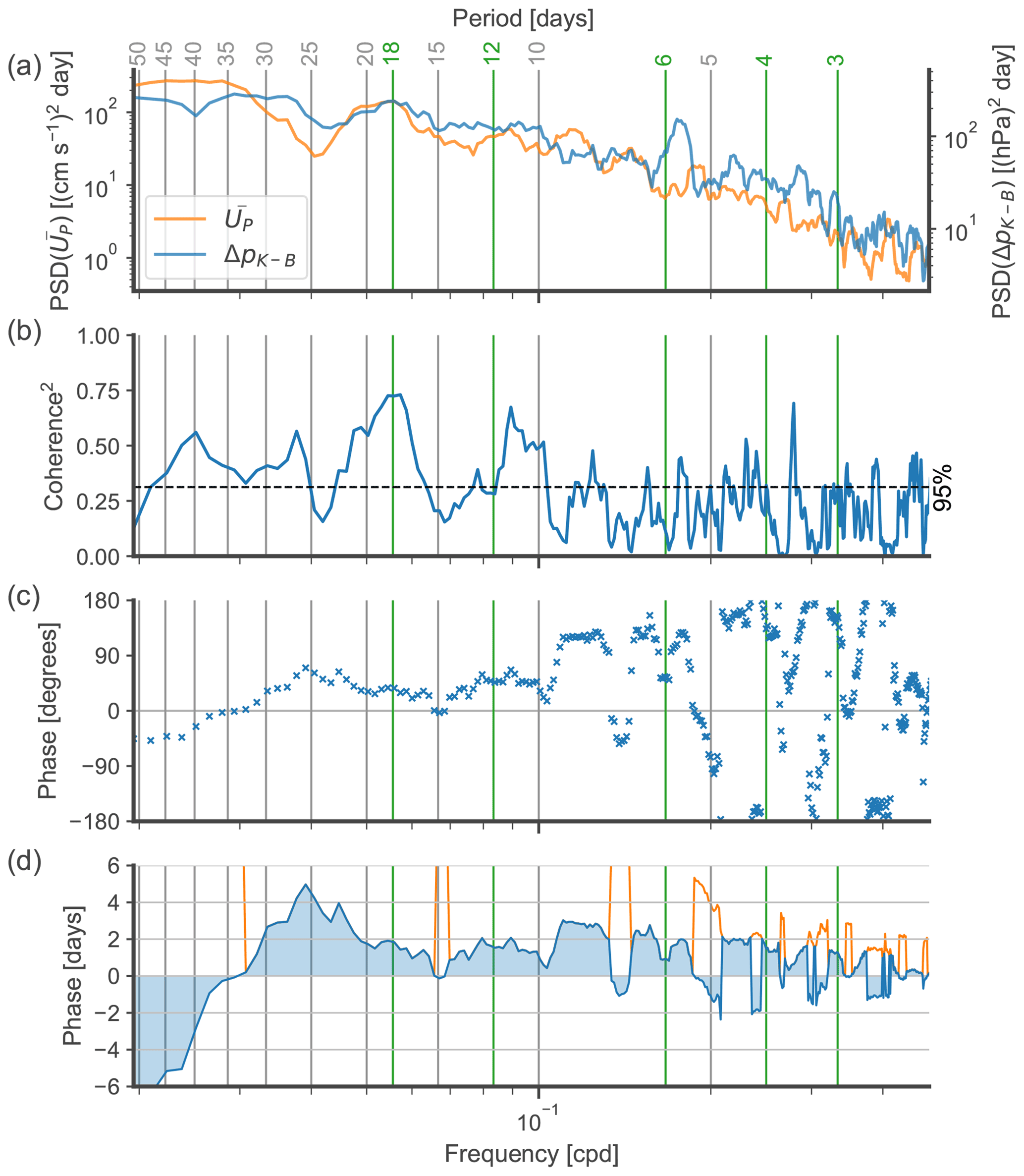
Figure A1(a) Power spectra of and ΔPK−B. (b) Coherence squared between the two variables, with the 95 % confidence interval shown as a dashed black line. (c) Coherence phase lag, with positive values indicating that ΔPK−B leads . (d) Coherence phase lag in units of days. The blue line shows the phase lag when the phase is allowed to be within . The orange line shows the lag in days when the phase is forced to be positive [], corresponding to ΔPK−B leading . In all panels, vertical grey lines indicate frequency values at equally spaced periods, and vertical green lines show frequencies of particular interest.
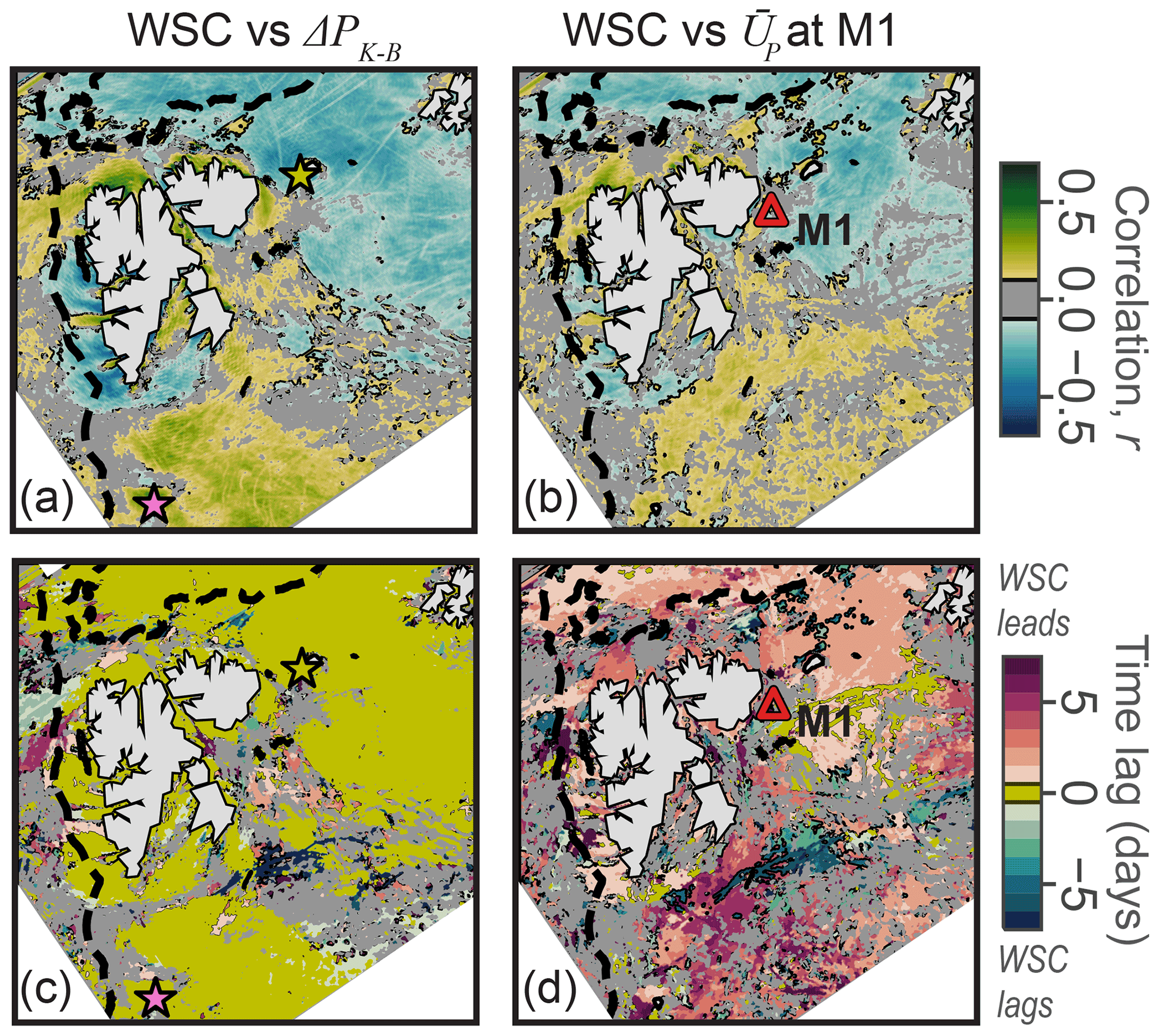
Figure A2Correlation between CARRA reanalysis wind stress curl and (a) ΔPK−B (positive for the low-pressure anomaly at Bjørnøya) and (b) at M1 (positive for flow towards the northeast). All variables have been high-pass-filtered by subtracting the 61 d running mean. Correlations were computed for lags between −7 and +7 d. Panels (c) and (d) show the lag at which maximum correlation shown in (a) and (b) is attained. Grey areas indicate where p>0.05 and/or . The 800 m bathymetric contour shown as a thick dashed line.
Data from the C3S Arctic Regional Reanalysis (Schyberg, 2020) were downloaded from the Copernicus Climate Change Service (C3S) Climate Data Store. AMSR2 sea ice concentration data (Spreen et al., 2008) were obtained from the University of Bremen Sea Ice Remote Sensing Data Centre (https://seaice.uni-bremen.de/start/data-archive/, last access 14 May 2021). Weather station data were obtained from the climate database of the Norwegian Meteorological Institute (accessed through https://www.eklima.no, last access: 21 May 2021). Shipboard CTD data from the KPH2019710 cruise (Sundfjord, 2022) are available through the Norwegian Marine Data Centre (https://nmdc.no/, last access 13 January 2022). Mooring data (Lundesgaard and Sundfjord, 2022; Sundfjord et al., 2022) have been made available through the Norwegian Polar Data Centre (https://data.npolar.no).
AS and AHHR designed the study, collected the data, and contributed comments to the paper. ØL performed the data processing and analysis, produced the figures, and wrote the initial draft of the paper. SL and FN contributed comments and discussion of importance to the subsequent development of the paper.
The contact author has declared that none of the authors has any competing interests.
Publisher's note: Copernicus Publications remains neutral with regard to jurisdictional claims in published maps and institutional affiliations.
The authors are grateful to NPI and IMR personnel, including captains and crews of the RV Kronprins Haakon, for technical support during the mooring cruises. Thanks are also extended to the two reviewers, whose constructive comments and suggestions resulted in substantial improvements to the paper.
The analysis was funded by the Research Council of Norway through the Nansen Legacy project (RCN 276730). Data collection was funded by Nansen Legacy as well as the Fram Centre project A-TWAIN (grant no. 66050) and the Research Council of Norway project SIOS-InfraNor (RCN 269927).
This paper was edited by Karen J. Heywood and reviewed by Yueng-Djern Lenn and one anonymous referee.
Aaboe, S., Lind, S., Hendricks, S., Down, E., Lavergne, T., and Ricker, R.: Sea-Ice and Ocean Conditions Surprisingly Normal in the Svalbard-Barents Sea Region after Large Sea-Ice Inflows in 2019, In: Copernicus Marine Service Ocean State Report, Issue 5, J. Oper. Ocean., 14, 140–148, https://doi.org/10.1080/1755876X.2021.1946240, 2021. a, b, c, d, e
Aagaard, K.: A Synthesis of the Arctic Ocean Circulation, Rapp. P. V. Reun. Cons. Int. Explor. Mer., 188, 11–22, 1989. a
Aagaard, K. and Greisman, P.: Toward New Mass and Heat Budgets for the Arctic Ocean, J. Geophys. Res., 80, 3821–3827, https://doi.org/10.1029/JC080i027p03821, 1975. a
Aagaard, K., Coachman, L. K., and Carmack, E.: On the Halocline of the Arctic Ocean, Deep Sea Res., 28, 529–545, https://doi.org/10.1016/0198-0149(81)90115-1, 1981. a, b, c
Ådlandsvik, B. and Loeng, H.: A Study of the Climatic System in the Barents Sea, Polar Res., 10, 45–50, https://doi.org/10.3402/polar.v10i1.6726, 1991. a
Aksenov, Y., Bacon, S., Coward, A. C., and Nurser, A. J. G.: The North Atlantic Inflow to the Arctic Ocean: High-resolution Model Study, J. Mar. Syst. 79, 1–22, https://doi.org/10.1016/j.jmarsys.2009.05.003, 2010. a, b, c
Årthun, M., Ingvaldsen, R. B., Smedsrud, L. H., and Schrum, C.: Dense Water Formation and Circulation in the Barents Sea, Deep Sea Res. Pt. I, 58, 801–817, https://doi.org/10.1016/j.dsr.2011.06.001, 2011. a
Årthun, M., Eldevik, T., Smedsrud, L. H., Skagseth, Ø., and Ingvaldsen, R. B.: Quantifying the Influence of Atlantic Heat on Barents Sea Ice Variability and Retreat, J. Climate, 25, 4736–4743, https://doi.org/10.1175/JCLI-D-11-00466.1, 2012. a, b
Athanase, M., Provost, C., Pérez-Hernández, M. D., Sennéchael, N., Bertosio, C., Artana, C., Garric, G., and Lellouche, J.-M.: Atlantic Water Modification North of Svalbard in the Mercator Physical System from 2007 to 2020, J. Geophys. Res.-Oceans, 125, e2020JC016463, https://doi.org/10.1029/2020JC016463, 2020. a, b
Barton, B. I., Lenn, Y.-D., and Lique, C.: Observed Atlantification of the Barents Sea Causes the Polar Front to Limit the Expansion of Winter Sea Ice, J. Phys. Ocean., 48, 1849–1866, https://doi.org/10.1175/JPO-D-18-0003.1, 2018. a
Beszczynska-Möller, A.: A Synthesis of Exchanges Through the Main Oceanic Gateways to the Arctic Ocean, Oceanography, 24, 82–99, https://doi.org/10.5670/oceanog.2011.59, 2011. a
Beszczynska-Möller, A., Fahrbach, E., Schauer, U., and Hansen, E.: Variability in Atlantic Water Temperature and Transport at the Entrance to the Arctic Ocean, 1997–2010, ICES J. Mar. Sci., 69, 852–863, https://doi.org/10.1093/icesjms/fss056, 2012. a
Carmack, E. C. and Kulikov, E. A.: Wind-Forced Upwelling and Internal Kelvin Wave Generation in Mackenzie Canyon, Beaufort Sea, J. Geophys. Res.-Oceans, 103, 18447–18458, https://doi.org/10.1029/98JC00113, 1998. a
Chulliat, A., Macmillan, S., Alken, P., Beggan, C., Nair, M., Hamilton, B., Woods, A., Ridley, V., Maus, S., and Thomson, A.: World Magnetic Model 2015, NOAA National Centers for Environmental Information, https://doi.org/10.7289/V5TH8JNW, 2014. a
Coachman, L. K. and Barnes, C. A.: The Movement of Atlantic Water in the Arctic Ocean, ARCTIC, 16, 8–16, https://doi.org/10.14430/arctic3517, 1963. a
Cole, S. T., Toole, J. M., Lele, R., Timmermans, M.-L., Gallaher, S. G., Stanton, T. P., Shaw, W. J., Hwang, B., Maksym, T., Wilkinson, J. P., Ortiz, M., Graber, H., Rainville, L., Petty, A. A., Farrell, S. L., Richter-Menge, J. A., and Haas, C.: Ice and Ocean Velocity in the Arctic Marginal Ice Zone: Ice Roughness and Momentum Transfer, Elementa, 5, 55, https://doi.org/10.1525/elementa.241, 2017. a
Copernicus Climate Change Service: Copernicus Arctic Regional ReAnalysis (CARRA), https://climate.copernicus.eu/copernicus-arctic-regional-reanalysis-service, last access: 5 December 2021.
Crews, L., Sundfjord, A., and Hattermann, T.: How the Yermak Pass Branch Regulates Atlantic Water Inflow to the Arctic Ocean, J. Geophys. Res.-Oceans, 124, 267–280, https://doi.org/10.1029/2018JC014476, 2019. a
Dalpadado, P., Arrigo, K. R., van Dijken, G. L., Skjoldal, H. R., Bagøien, E., Dolgov, A. V., Prokopchuk, I. P., and Sperfeld, E.: Climate Effects on Temporal and Spatial Dynamics of Phytoplankton and Zooplankton in the Barents Sea, Prog. Ocean., 185, 102320, https://doi.org/10.1016/j.pocean.2020.102320, 2020. a
Davis, R. E.: Predictability of Sea Surface Temperature and Sea Level Pressure Anomalies over the North Pacific Ocean, J. Phys. Ocean., 6, 249–266, https://doi.org/10.1175/1520-0485(1976)006<0249:POSSTA>2.0.CO;2, 1976. a
Dinniman, M. S. and Klinck, J. M.: A Model Study of Circulation and Cross-Shelf Exchange on the West Antarctic Peninsula Continental Shelf, Deep Sea Res. Pt. II, 51, 2003–2022, https://doi.org/10.1016/j.dsr2.2004.07.030, 2004. a
Docquier, D., Fuentes-Franco, R., Koenigk, T., and Fichefet, T.: Sea Ice–Ocean Interactions in the Barents Sea Modeled at Different Resolutions, Front. Earth Sci., 8, 172, https://doi.org/10.3389/feart.2020.00172, 2020. a
Dörr, J., Årthun, M., Eldevik, T., and Madonna, E.: Mechanisms of Regional Winter Sea-Ice Variability in a Warming Arctic, J. Climate, 34, 8635–8653, https://doi.org/10.1175/JCLI-D-21-0149.1, 2021. a
Erofeeva, S. Y. and Egbert, G.: Arc5km2018: Arctic Ocean Inverse Tide Model on a 5 Kilometer Grid, 2018, [data set], https://doi.org/10.18739/A21R6N14K, 2020. a
Fossheim, M., Primicerio, R., Johannesen, E., Ingvaldsen, R. B., Aschan, M. M., and Dolgov, A. V.: Recent Warming Leads to a Rapid Borealization of Fish Communities in the Arctic, Nat. Clim. Change, 5, 673–677, https://doi.org/10.1038/nclimate2647, 2015. a
Frainer, A., Primicerio, R., Kortsch, S., Aune, M., Dolgov, A. V., Fossheim, M., and Aschan, M. M.: Climate-Driven Changes in Functional Biogeography of Arctic Marine Fish Communities, P. Natl. Acad. Sci. USA, 114, 12202–12207, 2017. a
Furevik, T., Mauritzen, C., and Ingvaldsen, R.: The Flow of Atlantic Water to the Nordic Seas and Arctic Ocean, in: Arctic Alpine Ecosystems and People in a Changing Environment, edited by: Ørbæk, J. B., Kallenborn, R., Tombre, I., Hegseth, E. N., Falk-Petersen, S., and Hoel, A. H., Springer, Berlin, Heidelberg, 123–146, https://doi.org/10.1007/978-3-540-48514-8_8, 2007. a
Gelderloos, R., Haine, T. W. N., and Almansi, M.: Coastal Trapped Waves and Other Subinertial Variability along the Southeast Greenland Coast in a Realistic Numerical Simulation, J. Phys. Ocean., 51, 861–877, https://doi.org/10.1175/JPO-D-20-0239.1, 2021. a
Guest, P. S. and Davidson, K. L.: The Effect of Observed Ice Conditions on the Drag Coefficient in the Summer East Greenland Sea Marginal Ice Zone, J. Geophys. Res.-Oceans, 92, 6943–6954, https://doi.org/10.1029/JC092iC07p06943, 1987. a
Hakkinen, S. and Rhines, P. B.: Shifting Surface Currents in the Northern North Atlantic Ocean, J. Geophys. Res.-Oceans, 114, C04005, https://doi.org/10.1029/2008JC004883, 2009. a
Hansen, B. and Østerhus, S.: North Atlantic–Nordic Seas Exchanges, Prog. Oceanogr., 45, 109–208, https://doi.org/10.1016/S0079-6611(99)00052-X, 2000. a
Harris, C. L., Plueddemann, A. J., and Gawarkiewicz, G. G.: Water Mass Distribution and Polar Front Structure in the Western Barents Sea, J. Geophys. Res.-Oceans, 103, 2905–2917, https://doi.org/10.1029/97JC02790, 1998. a, b
Holliday, N. P., Cunningham, S. A., Johnson, C., Gary, S. F., Griffiths, C., Read, J. F., and Sherwin, T.: Multidecadal Variability of Potential Temperature, Salinity, and Transport in the Eastern Subpolar North Atlantic, J. Geophys. Res.-Oceans, 120, 5945–5967, https://doi.org/10.1002/2015JC010762, 2015. a
Inall, M. E., Nilsen, F., Cottier, F. R., and Daae, R.: Shelf/Fjord Exchange Driven by Coastal-Trapped Waves in the Arctic, J. Geophys. Res.-Oceans, 120, 8283–8303, https://doi.org/10.1002/2015JC011277, 2015. a, b
Ingvaldsen, R., Loeng, H., and Asplin, L.: Variability in the Atlantic Inflow to the Barents Sea Based on a One-Year Time Series from Moored Current Meters, Cont. Shelf Res., 22, 505–519, https://doi.org/10.1016/S0278-4343(01)00070-X, 2002. a, b
Ingvaldsen, R. B., Assmann, K. M., Primicerio, R., Fossheim, M., Polyakov, I. V., and Dolgov, A. V.: Physical Manifestations and Ecological Implications of Arctic Atlantification, Nat. Rev. Earth Environ., 2.12, 874–889, 2021. a, b, c
Ivanov, V. V., Polyakov, I. V., Dmitrenko, I. A., Hansen, E., Repina, I. A., Kirillov, S. A., Mauritzen, C., Simmons, H., and Timokhov, L. A.: Seasonal Variability in Atlantic Water off Spitsbergen, Deep Sea Res. Pt. I, 56, 1–14, https://doi.org/10.1016/j.dsr.2008.07.013, 2009. a, b
Jakobsson, M., Mayer, L., Coakley, B., Dowdeswell, J. A., Forbes, S., Fridman, B., Hodnesdal, H., Noormets, R., Pedersen, R., Rebesco, M., Schenke, H. W., Zarayskaya, Y., Accettella, D., Armstrong, A., Anderson, R. M., Bienhoff, P., Camerlenghi, A., Church, I., Edwards, M., Gardner, J. V., Hall, J. K., Hell, B., Hestvik, O., Kristoffersen, Y., Marcussen, C., Mohammad, R., Mosher, D., Nghiem, S. V., Pedrosa, M. T., Travaglini, P. G., and Weatherall, P.: The International Bathymetric Chart of the Arctic Ocean (IBCAO) Version 3.0, Geophys. Res. Lett., 39, L12609, https://doi.org/10.1029/2012GL052219, 2012. a
Johannesen, E., Jørgensen, L. L., Fossheim, M., Primicerio, R., Greenacre, M., Ljubin, P. A., Dolgov, A. V., Ingvaldsen, R. B., Anisimova, N. A., and Manushin, I. E.: Large-Scale Patterns in Community Structure of Benthos and Fish in the Barents Sea, Polar Biol., 40, 237–246, https://doi.org/10.1007/s00300-016-1946-6, 2017. a
Jones, E. P.: Circulation in the Arctic Ocean, Polar Res., 20, 139–146, https://doi.org/10.1111/j.1751-8369.2001.tb00049.x, 2001. a
Jordi, A., Klinck, J. M., Basterretxea, G., Orfila, A., and Tintoré, J.: Estimation of Shelf-Slope Exchanges Induced by Frontal Instability near Submarine Canyons, J. Geophys. Res.-Oceans, 113, C05016, https://doi.org/10.1029/2007JC004207, 2008. a
Kämpf, J.: Transient Wind-Driven Upwelling in a Submarine Canyon: A Process-Oriented Modeling Study, J. Geophys. Res.-Oceans, 111, C11011, https://doi.org/10.1029/2006JC003497, 2006. a, b
Kämpf, J. and Chapman, P.: The Functioning of Coastal Upwelling Systems, in: Upwelling Systems of the World: A Scientific Journey to the Most Productive Marine Ecosystems, edited by: Kämpf, J. and Chapman, P., Springer International Publishing, Cham, 31–65, https://doi.org/10.1007/978-3-319-42524-5_2, 2016. a
Koenig, Z., Provost, C., Sennéchael, N., Garric, G., and Gascard, J.-C.: The Yermak Pass Branch: A Major Pathway for the Atlantic Water North of Svalbard?, J. Geophys. Res.-Oceans, 122, 9332–9349, https://doi.org/10.1002/2017JC013271, 2017. a
Kolås, E. H., Koenig, Z., Fer, I., Nilsen, F., and Marnela, M.: Structure and Transport of Atlantic Water North of Svalbard From Observations in Summer and Fall 2018, J. Geophys. Res.-Oceans, 125, e2020JC016174, https://doi.org/10.1029/2020JC016174, 2020. a, b
Kortsch, S., Primicerio, R., Fossheim, M., Dolgov, A. V., and Aschan, M.: Climate Change Alters the Structure of Arctic Marine Food Webs Due to Poleward Shifts of Boreal Generalists, P. Roy. Soc. B-Bio., 282, 20151546, 2015. a
Kortsch, S., Primicerio, R., Aschan, M., Lind, S., Dolgov, A. V., and Planque, B.: Food-Web Structure Varies along Environmental Gradients in a High-Latitude Marine Ecosystem, Ecography, 42, 295–308, 2019. a
Large, W. G. and Pond, S.: Open Ocean Momentum Flux Measurements in Moderate to Strong Winds, J. Phys. Ocean., 11, 324–336, https://doi.org/10.1175/1520-0485(1981)011<0324:OOMFMI>2.0.CO;2, 1981. a
Lewis, K. M., van Dijken, G. L., and Arrigo, K. R.: Changes in Phytoplankton Concentration Now Drive Increased Arctic Ocean Primary Production, Science, 369, 198–202, https://doi.org/10.1126/science.aay8380, 2020. a
Li, H., Chen, H., Wang, H., Sun, J., and Ma, J.: Can Barents Sea Ice Decline in Spring Enhance Summer Hot Drought Events over Northeastern China?, J. Climate, 31, 4705–4725, https://doi.org/10.1175/JCLI-D-17-0429.1, 2018. a
Lien, V. S., Vikebø, F. B., and Skagseth, Ø.: One Mechanism Contributing to Co-Variability of the Atlantic Inflow Branches to the Arctic, Nat. Commun., 4, 1488, https://doi.org/10.1038/ncomms2505, 2013. a
Lien, V. S., Schlichtholz, P., Skagseth, Ø., and Vikebø, F. B.: Wind-Driven Atlantic Water Flow as a Direct Mode for Reduced Barents Sea Ice Cover, J. Climate, 30, 803–812, https://doi.org/10.1175/JCLI-D-16-0025.1, 2017.
Lind, S. and Ingvaldsen, R. B.: Variability and Impacts of Atlantic Water Entering the Barents Sea from the North, Deep Sea Res. Pt. I, 62, 70–88, https://doi.org/10.1016/j.dsr.2011.12.007, 2012. a, b, c, d, e, f
Lind, S., Ingvaldsen, R. B., and Furevik, T.: Arctic Layer Salinity Controls Heat Loss from Deep Atlantic Layer in Seasonally Ice-Covered Areas of the Barents Sea, Geophys. Res. Lett., 43, 5233–42, https://doi.org/10.1002/2016GL068421, 2016. a
Lind, S., Ingvaldsen, R. B., and Furevik, T.: Arctic Warming Hotspot in the Northern Barents Sea Linked to Declining Sea-Ice Import, Nat. Clim. Change, 8, 634–639, https://doi.org/10.1038/s41558-018-0205-y, 2018. a, b, c, d, e, f, g
Lique, C. and Steele, M.: Where Can We Find a Seasonal Cycle of the Atlantic Water Temperature within the Arctic Basin?, J. Geophys. Res.-Oceans, 117, C03026, https://doi.org/10.1029/2011JC007612, 2012. a
Loeng, H.: Features of the Physical Oceanographic Conditions of the Barents Sea, Polar Res., 10, 5–18, https://doi.org/10.3402/polar.v10i1.6723, 1991. a, b, c, d, e, f, g
Loeng, H., Ozhigin, V., and Ådlandsvik, B.: Water Fluxes through the Barents Sea, ICES J. Mar. Sci., 54, 310–317, https://doi.org/10.1006/jmsc.1996.0165, 1997. a
Løyning, T. B.: Hydrography in the North–Western Barents Sea, July–August 1996, Polar Res., 20, 1–11, https://doi.org/10.1111/j.1751-8369.2001.tb00034.x, 2001. a
Lundesgaard, Ø., Sundfjord, A., and Renner, A. H. H.: Drivers of Interannual Sea Ice Concentration Variability in the Atlantic Water Inflow Region North of Svalbard, J. Geophys. Res.-Oceans, 126, e2020JC016522, https://doi.org/10.1029/2020JC016522, 2021. a, b
Lundesgaard, Ø., Sundfjord, A.: Time series of ocean currents, temperature, salinity, and pressure from ocean moorings M1 and M2 in the northwestern Barents Sea [data set], Norwegian Polar Institute, https://doi.org/10.21334/npolar.2022.1a68b156, 2022. a
Madonna, E., Hes, G., Li, C., Michel, C., and Siew, P. Y. F.: Control of Barents Sea Wintertime Cyclone Variability by Large-Scale Atmospheric Flow, Geophys. Res. Lett., 47, e2020GL090322, https://doi.org/10.1029/2020GL090322, 2020. a
Martin, T., Steele, M., and Zhang, J.: Seasonality and Long-Term Trend of Arctic Ocean Surface Stress in a Model, J. Geophys. Res.-Oceans, 119, 1723–1738, https://doi.org/10.1002/2013JC009425, 2014. a
Matishov, G. G., Matishov, D. G., and Moiseev, D. V.: Inflow of Atlantic-origin Waters to the Barents Sea along Glacial Troughs, Oceanologia, 51, 321–340, 2009. a, b
Mauritzen, C.: Production of Dense Overflow Waters Feeding the North Atlantic across the Greenland-Scotland Ridge, Part 1: Evidence for a Revised Circulation Scheme, Deep Sea Res. Pt. I, 43, 769–806, https://doi.org/10.1016/0967-0637(96)00037-4, 1996. a
Menze, S., Ingvaldsen, R. B., Nikolopoulos, A., Hattermann, T., Albretsen, J., and Gjøsæter, H.: Productive Detours – Atlantic Water Inflow and Acoustic Backscatter in the Major Troughs along the Svalbard Shelf, Prog. Oceanogr., 188, 102447, https://doi.org/10.1016/j.pocean.2020.102447, 2020. a, b
Midttun, L.: Formation of Dense Bottom Water in the Barents Sea, Deep Sea Res., 32, 1233–1241, https://doi.org/10.1016/0198-0149(85)90006-8, 1985. a
Mosby, H.: Svalbard Waters, Geophys. Publ., 12, 1–86, 1938. a, b, c, d
Mosby, H.: Water, Salt and Heat Balance of the North Polar Sea and of the Norwegian Sea, Geophys. Norveg., 24, 289–313, 1962. a
Mysak, L. A.: Topographically Trapped Waves, Annual Review of Fluid Mechanics, 12, 45–76, https://doi.org/10.1146/annurev.fl.12.010180.000401, 1980. a
Nansen, F.: The Oceanography of the North Polar Basin. The Norwegian North Polar Expedition 1893-1896., Scient. Results, 3 (9), 1902. a
Nilsen, F., Skogseth, R., Vaardal-Lunde, J., and Inall, M.: A Simple Shelf Circulation Model: Intrusion of Atlantic Water on the West Spitsbergen Shelf, J. Phys. Ocean., 46, 1209–1230, https://doi.org/10.1175/JPO-D-15-0058.1, 2016. a, b, c
Nøst, O. A., Nilsson, J., and Nycander, J.: On the Asymmetry between Cyclonic and Anticyclonic Flow in Basins with Sloping Boundaries, J. Phys. Ocean.,, 38, 771–787, https://doi.org/10.1175/2007JPO3714.1, 2008. a
Onarheim, I. H. and Årthun, M.: Toward an Ice-Free Barents Sea, Geophys. Res. Lett., 44, 8387–8395, https://doi.org/10.1002/2017GL074304, 2017. a
Onarheim, I. H., Smedsrud, L. H., Ingvaldsen, R. B., and Nilsen, F.: Loss of Sea Ice during Winter North of Svalbard, Tellus A, 66, 23933, https://doi.org/10.3402/tellusa.v66.23933, 2014. a
Oziel, L., Sirven, J., and Gascard, J.-C.: The Barents Sea Frontal Zones and Water Masses Variability (1980–2011), Ocean Sci., 12, 169–184, https://doi.org/10.5194/os-12-169-2016, 2016. a, b
Pérez-Hernández, M. D., Pickart, R. S., Pavlov, V., Våge, K., Ingvaldsen, R., Sundfjord, A., Renner, A. H. H., Torres, D. J., and Erofeeva, S. Y.: The Atlantic Water Boundary Current North of Svalbard in Late Summer, J. Geophys. Res.-Oceans, 122, 2269–2290, https://doi.org/10.1002/2016JC012486, 2017. a, b, c
Pérez-Hernández, M. D., Pickart, R. S., Torres, D. J., Bahr, F., Sundfjord, A., Ingvaldsen, R., Renner, A. H. H., Beszczynska-Möller, A., von Appen, W.-J., and Pavlov, V.: Structure, Transport, and Seasonality of the Atlantic Water Boundary Current North of Svalbard: Results From a Yearlong Mooring Array, J. Geophys. Res.-Oceans, 124, 1679–1698, https://doi.org/10.1029/2018JC014759, 2019. a
Petoukhov, V. and Semenov, V. A.: A Link between Reduced Barents-Kara Sea Ice and Cold Winter Extremes over Northern Continents, J. Geophys. Res.-Atmos., 115, D21111, https://doi.org/10.1029/2009JD013568, 2010. a
Pfirman, S., Bauch, D., and Gammelsrød, T.: The Northern Barents Sea: Water Mass Distribution and Modification, in: The Polar Oceans and Their Role in Shaping the Global Environment, edited by: Johannessen, O. M., Muench, R. D., and Overland, J. E., AGU, Ameircan Geophysical Union, Washington, DC, USA, 77–94, https://doi.org/10.1029/GM085p0077, 1994. a, b
Phillips, N. A.: Geostrophic Motion, Rev. Geophys., 1, 123–176, https://doi.org/10.1029/RG001i002p00123, 1963. a
Pnyushkov, A. V., Polyakov, I. V., Ivanov, V. V., Aksenov, Y., Coward, A. C., Janout, M., and Rabe, B.: Structure and Variability of the Boundary Current in the Eurasian Basin of the Arctic Ocean, Deep Sea Res. Pt. I, 101, 80–97, https://doi.org/10.1016/j.dsr.2015.03.001, 2015. a
Polyakov, I. V., Pnyushkov, A. V., Alkire, M. B., Ashik, I. M., Baumann, T. M., Carmack, E. C., Goszczko, I., Guthrie, J., Ivanov, V. V., Kanzow, T., Krishfield, R., Kwok, R., Sundfjord, A., Morison, J., Rember, R., and Yulin, A.: Greater Role for Atlantic Inflows on Sea-Ice Loss in the Eurasian Basin of the Arctic Ocean, Science, 356, 285–291, https://doi.org/10.1126/science.aai8204, 2017. a
Randelhoff, A. and Sundfjord, A.: Short Commentary on Marine Productivity at Arctic Shelf Breaks: Upwelling, Advection and Vertical Mixing, Ocean Sci., 14, 293–300, https://doi.org/10.5194/os-14-293-2018, 2018. a
Renner, A. H. H., Sundfjord, A., Janout, M. A., Ingvaldsen, R. B., Beszczynska-Möller, A., Pickart, R. S., and Pérez-Hernández, M. D.: Variability and Redistribution of Heat in the Atlantic Water Boundary Current North of Svalbard, J. Geophys. Res.-Oceans, 123, 6373–6391, https://doi.org/10.1029/2018JC013814, 2018. a, b, c, d, e, f, g
Rudels, B.: Arctic Ocean Circulation, Processes and Water Masses: A Description of Observations and Ideas with Focus on the Period Prior to the International Polar Year 2007–2009, Prog. Oceanogr., 132, 22–67, https://doi.org/10.1016/j.pocean.2013.11.006, 2015. a
Saldías, G. S., Ramos-Musalem, K., and Allen, S. E.: Circulation and Upwelling Induced by Coastal Trapped Waves over a Submarine Canyon in an Idealized Eastern Boundary Margin, Geophys. Res. Lett., 48, e2021GL093548, https://doi.org/10.1029/2021GL093548, 2021. a
Schauer, U., Loeng, H., Rudels, B., Ozhigin, V. K., and Dieck, W.: Atlantic Water Flow through the Barents and Kara Seas, Deep Sea Res. Pt. I, 49, 2281–2298, https://doi.org/10.1016/S0967-0637(02)00125-5, 2002. a, b, c
She, J. and Klinck, J. M.: Flow near Submarine Canyons Driven by Constant Winds, J. Geophys. Res.-Oceans, 105, 28671–28694, https://doi.org/10.1029/2000JC900126, 2000. a
Schyberg, H., Yang, X., Køltzow, M. A. Ø., Amstrup, B., Bakketun, Å., Bazile, E., Bojarova, J., Box, J. E., Dahlgren, P., Hagelin, S., Homleid, M., Horányi, A., Høyer, J., Johansson, Å., Killie, M. A., Körnich, H., Le Moigne, P., Lindskog, M., Manninen, T., Nielsen Englyst, P., Nielsen, K. P., Olsson, E., Palmason, B., Peralta Aros, C., Randriamampianina, R., Samuelsson, P., Stappers, R, Støylen, E., Thorsteinsson, S., Valkonen, T., Wang, Z. Q.: Arctic Regional Reanalysis on Single Levels from 1991 to Present, Copernicus Climate Change Service (C3S) Climate Data Store (CDS), https://doi.org/10.24381/cds.713858f6, 2020. a, b
Skagseth, Ø.: Recirculation of Atlantic Water in the Western Barents Sea, Geophys. Res. Lett., 35, L11606, https://doi.org/10.1029/2008GL033785, 2008. a
Smedsrud, L. H., Esau, I., Ingvaldsen, R. B., Eldevik, T., Haugan, P. M., Li, C., Lien, V. S., Olsen, A., Omar, A. M., Otterå, O. H., Risebrobakken, B., Sandø, A. B., Semenov, V. A., and Sorokina, S. A.: The Role of the Barents Sea in the Arctic Climate System, Rev. Geophys., 51, 415–449, https://doi.org/10.1002/rog.20017, 2013. a, b, c
Sorteberg, A. and Kvingedal, B.: Atmospheric Forcing on the Barents Sea Winter Ice Extent, J. Climate, 19, 4772–4784, https://doi.org/10.1175/JCLI3885.1, 2006. a
Spence, P., Holmes, R. M., Hogg, A. M., Griffies, S. M., Stewart, K. D., and England, M. H.: Localized Rapid Warming of West Antarctic Subsurface Waters by Remote Winds, Nat. Clim. Change, 7, 595–603, https://doi.org/10.1038/nclimate3335, 2017. a
Spreen, G., Kaleschke, L., and Heygster, G.: Sea Ice Remote Sensing Using AMSR-E 89-GHz Channels, J. Geophys. Res.-Oceans, 113, C02S03, https://doi.org/10.1029/2005JC003384, 2008. a, b
Sternberg, R. W., Aagaard, K., Cacchione, D., Wheatcroft, R. A., Beach, R. A., Roach, A. T., and Marsden, M. A. H.: Long-Term near-Bed Observations of Velocity and Hydrographic Properties in the Northwest Barents Sea with Implications for Sediment Transport, Cont. Shelf Res., 21, 267–287, https://doi.org/10.1016/S0278-4343(00)00103-5, 2001. a, b
Sundfjord, A.: CTD data from Nansen Legacy Cruise – Mooring service cruise 2019, [data set], https://doi.org/10.21335/NMDC-2135074338, 2022. a
Sundfjord, A., Assmann, K. M., Lundesgaard, Ø., Renner, A. H. H., Lind, S., and Ingvaldsen, R. B.: Suggested Water Mass Definitions for the Central and Northern Barents Sea, and the Adjacent Nansen Basin:, The Nansen Legacy Report Series, https://doi.org/10.7557/nlrs.5707, 2020. a, b
Sundfjord, A., Lundesgaard, Ø., and Renner, A. H.: A-TWAIN mooring data 2019–2020 [data set], Norwegian Polar Institute, https://doi.org/10.21334/npolar.2022.d3a5adc2, 2022. a
Timmermans, M.-L. and Marshall, J.: Understanding Arctic Ocean Circulation: A Review of Ocean Dynamics in a Changing Climate, J. Geophys. Res.-Oceans, 125, e2018JC014378, https://doi.org/10.1029/2018JC014378, 2020. a, b, c
Torres-Valdés, S., Tsubouchi, T., Bacon, S., Naveira-Garabato, A. C., Sanders, R., McLaughlin, F. A., Petrie, B., Kattner, G., Azetsu-Scott, K., and Whitledge, T. E.: Export of Nutrients from the Arctic Ocean, J. Geophys. Res.-Oceans, 118, 1625–1644, 2013. a
Våge, K., Pickart, R. S., Pavlov, V., Lin, P., Torres, D. J., Ingvaldsen, R., Sundfjord, A., and Proshutinsky, A.: The Atlantic Water Boundary Current in the Nansen Basin: Transport and Mechanisms of Lateral Exchange, J. Geophys. Res.-Oceans, 121, 6946–6960, https://doi.org/10.1002/2016JC011715, 2016. a
von Appen, W.-J.: Correction of ADCP Compass Errors Resulting from Iron in the Instrument's Vicinity, J. Atmos. Ocean. Tech., 32, 591–602, https://doi.org/10.1175/JTECH-D-14-00043.1, 2015. a
Wassmann, P., Kosobokova, K. N., Slagstad, D., Drinkwater, K. F., Hopcroft, R. R., Moore, S. E., Ellingsen, I., Nelson, R. J., Carmack, E., Popova, E., and Berge, J.: The Contiguous Domains of Arctic Ocean Advection: Trails of Life and Death, Prog. Oceanogr., 139, 42–65, https://doi.org/10.1016/j.pocean.2015.06.011, 2015. a
Wickström, S., Jonassen, M. O., Vihma, T., and Uotila, P.: Trends in Cyclones in the High-Latitude North Atlantic during 1979–2016, Q. J. Roy. Meteor. Soc., 146, 762–779, https://doi.org/10.1002/qj.3707, 2020. a, b
Woodgate, R. A., Aagaard, K., Muench, R. D., Gunn, J., Björk, G., Rudels, B., Roach, A. T., and Schauer, U.: The Arctic Ocean Boundary Current along the Eurasian Slope and the Adjacent Lomonosov Ridge: Water Mass Properties, Transports and Transformations from Moored Instruments, Deep Sea Res. Pt. I, 48, 1757–1792, https://doi.org/10.1016/S0967-0637(00)00091-1, 2001. a