the Creative Commons Attribution 4.0 License.
the Creative Commons Attribution 4.0 License.
 | 14 Sep 2022
Hydrography, circulation, and response to atmospheric forcing in the vicinity of the central Getz Ice Shelf, Amundsen Sea, Antarctica
Vår Dundas
Elin Darelius
Kjersti Daae
Nadine Steiger
Yoshihiro Nakayama
Tae-Wan Kim
Ice shelves in the Amundsen Sea are thinning rapidly as ocean currents bring warm water into the cavities beneath the floating ice. Although the reported melt rates for the Getz Ice Shelf are comparatively low for the region, its size makes it one of the largest freshwater sources around Antarctica, with potential consequences for, bottom water formation downstream, for example. Here, we use a 2-year-long novel mooring record (2016–2018) and 16-year-long regional model simulations to describe, for the first time, the hydrography and circulation in the vicinity of the ice front between Siple and Carney Island. We find that, throughout the mooring record, temperatures in the trough remain below 0.15 ∘C, more than 1 ∘C lower than in the neighboring Siple and Dotson Trough, and we observe a mean current (0.03 m s−1) directed toward the ice shelf front. The variability in the heat transport toward the ice shelf appears to be governed by nonlocal ocean surface stress over the Amundsen Sea Polynya region, and northward to the continental shelf break, where strengthened westward ocean surface stress leads to increased southward flow at the mooring site. The model simulations suggest that the heat content in the trough during the observed period was lower than normal, possibly owing to anomalously low summertime sea ice concentration and weak winds.
- Article
(9102 KB) - Full-text XML
- BibTeX
- EndNote


The Getz Ice Shelf (GIS) in the western Amundsen Sea is among Antarctica's primary sources of meltwater (Rignot et al., 2013) and one of the main contributors of ice shelf volume loss (Paolo et al., 2015), with basal melt rates approaching 5 m yr−1 (Rignot et al., 2013). Despite the stabilizing buttressing effect of islands that separate its ice fronts (Fig. 1a, e.g., Heywood et al., 2016; Shepherd et al., 2018; Jacobs et al., 2013; Dupont and Alley, 2005), the GIS grounding line is retreating (Shepherd et al., 2018), potentially influencing the stability of the GIS. The high melt rates enhance the meltwater fraction transported from the GIS and westward to the Ross Sea (Nakayama et al., 2014a, 2020), connecting changes in the GIS region to the global climate: More meltwater in the Ross Sea is suggested to affect the Antarctic Bottom Water production and the global thermohaline circulation, and consequently the global ocean overturning (Nakayama et al., 2014a, b). Despite this connection between the ocean-driven melt of the GIS and the global climate, the area is severely undersampled.
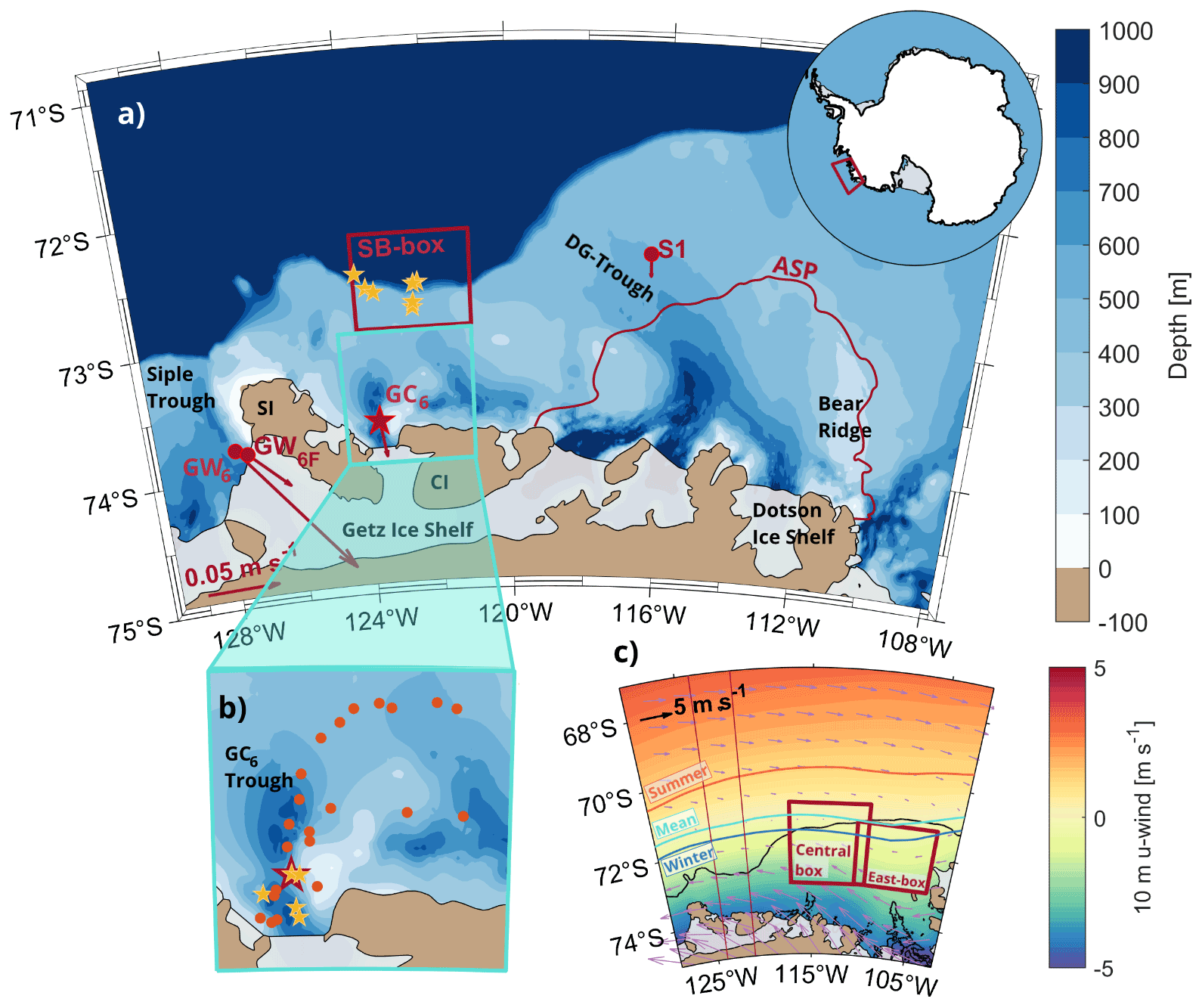
Figure 1(a) Map of the Amundsen Sea with bathymetry (color scale) (IBCSO, Arndt et al., 2013) and ice shelf (gray) (Bedmap2, Fretwell et al., 2013). The location of the study region within Antarctica is indicated by a red box in the inset. The moorings GC6 (red star), GW6, GW6F, and S1 (red dots) are marked, with arrows denoting mean current averaged over depth and time. The velocity scale is given in the lower left corner. SI: Siple Island, CI: Carney Island, ASP: Amundsen Sea Polynya, and DG Trough: Dotson–Getz Trough. The outline of the ASP is based on data from January 2011 (Yager et al., 2012). (b) Detailed map of the GC6 trough. Conductivity, temperature, and depth (CTD) stations from ship-borne surveys (yellow stars) are shown in (a) and (b). CTD stations from an instrumented seal are marked with orange dots. (c) The mean wind field from 2001 to 2018 (ERA 5, color scale and purple arrows, see black arrow for scale) with mean zero-contours during the 17-year period (cyan), summer (red), and winter (blue). The thin meridional red lines indicate the meridional band used for estimating the latitude of the zero-contour north of GC6. The black contour is the 900-m isobaths. The red SB (a), ASP, and East boxes (c) indicate regions used for averaging ocean surface stress. The SB box is also used for estimating cumulative Ekman pumping anomalies.
The presence of warm and dense Circumpolar Deep Water (CDW, core temperature of 2 ∘C, Heywood et al., 2016) and its slightly colder modified version (mCDW) on the continental shelf is the main cause of the high basal melt rates in the Amundsen Sea (Rignot et al., 2019). CDW is found just off-shelf of the continental shelf break, a characteristic specific to West Antarctica (e.g., Holland et al., 2020). However, the Getz region's regional differences are large (Jacobs et al., 2013). The GIS spans roughly 650 km along the coast (Jacobs et al., 2013) and is sectioned into several ice shelf fronts by six islands (Assmann et al., 2019). The differences in local bathymetry, variations in the regional wind field, the Antarctic Slope Front (ASF), an along-slope undercurrent, and the depth of the thermocline relative to the ice shelf grounding lines cause a spatially inhomogeneous ice thickness change within the Amundsen Sea (Paolo et al., 2015; Shepherd et al., 2018). Together, these aspects influence whether the CDW from the deep ocean is allowed onto the continental shelf and whether it reaches the ice shelf bases to the south. Different combinations of the mechanisms that admit on-shelf heat transport dominate at different locations, and consequently, each GIS frontal region needs to be studied separately.
In this paper, we present the first mooring record, GC6 (Getz Central, 650 m, 2016–2018, Fig. 1a), near the GIS front between Siple and Carney Islands. This trough (referred to as the GC6 Trough hereafter) has until now been overlooked, compared with the neighboring Siple Trough in the west, and the Dotson–Getz Trough in the east, which have recently received attention (Assmann et al., 2019; Wåhlin et al., 2020a; Steiger et al., 2021; Wåhlin et al., 2010, 2013; Kalén et al., 2016; Dotto et al., 2020). Historically, few observations exist from the GC6 Trough, and consequently, our new mooring observations enable a first detailed description of the oceanography in the trough, beyond previous descriptions based on snapshot conductivity, temperature, and depth (CTD) measurements (Jacobs et al., 2013).
The surface winds drive a wide range of processes that affect on-shelf heat transport, such as Ekman pumping at the shelf break (Assmann et al., 2019), on-shelf current variability (Wåhlin et al., 2013), and the on-shelf flow of CDW (Thoma et al., 2008). The winds are predominantly westward along the coast and eastward north of the shelf break. The latitude where these zonal winds shift direction, the “zero-contour,” generally migrates northward in summer and southward in winter (Assmann et al., 2013). Although the eastern part of the Amundsen Sea shelf break experiences a seasonal shift in zonal winds, the western part is usually affected by westward winds year-round owing to its higher latitude.
Variations in the ASF, the associated Antarctic Slope Current (ASC), and its undercurrent are related to these wind patterns (Dotto et al., 2019). The ASF is a wind-driven frontal system at the continental shelf break (Jacobs, 1991). Its associated sharp thermocline and downward-sloping isotherms from north to south impede the flow of CDW across the shelf break (e.g., Thompson et al., 2018), and consequently regulate the amount of heat on the continental shelf. Westward winds sharpen the ASF through downward Ekman pumping (e.g., Thompson et al., 2018), whereas surface stratification dampens this effect and relaxes the ASF (Daae et al., 2017). The eastward undercurrent is maintained by the horizontal density gradients across the ASF (e.g., Smedsrud et al., 2006; Chavanne et al., 2010). When the isopycnals of the ASF are steep enough to sustain the undercurrent and relaxed enough to admit water below the thermocline over the trough sills, this undercurrent brings warm water directly into troughs (Walker et al., 2013; Assmann et al., 2013).
While the adjacent Siple and Dotson–Getz Troughs cross-cut the continental shelf (Fig. 1a), the GC6 Trough does not reach the shelf break, although it is ∼1000 m deep at the ice front (Fig. 2c). In addition, the shallow sill-region north of GC6 is likely accompanied by a relatively deep thermocline (Jacobs et al., 2012). The warm along-slope undercurrent (Walker et al., 2013; Assmann et al., 2013; Dotto et al., 2019) may therefore cross the deep Siple and Dotson–Getz Trough sills (∼570 and ∼500 m deep), but not the shallower GC6 Trough's sill (∼460 m deep). However, unmodified CDW is present directly north of the GC6 Trough sill (Fig. 3b), and water roughly 2 ∘C above freezing was observed in the GC6 Trough by a snapshot CTD in 2007 (Jacobs et al., 2013).
We describe the observed hydrography and currents at GC6 based on the mooring records and compare the observations with those from neighboring troughs (Siple and Dotson-Getz). We discuss their variability and possible drivers, with a specific focus on forcing by ocean surface stress (τ). To set the 2 years of mooring observations in a broader temporal and spatial perspective and compensate for the sparse observational data coverage, we investigate output from a high-resolution regional model run (Nakayama et al., 2018) and include historical CTD data from the trough.
2.1 Observational data
The mooring GC6 was deployed during the Amundsen Sea Expedition 2015–2016 (ANA06B) and collected data from 30 January 2016 to 31 January 2018. It was located at a depth of 648 m on the eastern slope of the GC6 Trough (123.6∘ W, 73.7∘ S), about 30 km north of one of the GIS's ice fronts (Fig. 1a, b). GC6 recorded temperature, salinity, pressure (SBE56 and SBE37 from Seabird Electronics), and current velocity (RDI ADCP, 150 kHz, for instrument levels see Fig. 2b). The data are corrected for magnetic declination, outliers are removed, and the ADCP data are processed with the RDI software following standard procedures. We use hourly and daily averaged data of all variables. We follow TEOS-10 (IOC et al., 2010) and present the hydrographic data as absolute salinity (SA) and conservative temperature (Θ) with δSA taken from version 3.6 of McDougall et al.'s (2012) database.

Figure 2(a) Profiles of conservative temperature (orange) and absolute salinity (blue) obtained from CTD casts at deployment (thick lines) and recovery (thin lines) of mooring GC6. Mean temperature (orange diamonds) and salinity (blue squares) recorded by each instrument on GC6 with standard deviation (black lines) is marked. The standard deviation for salinity is too small to be seen outside the blue boxes. (b) Instrument levels for temperature, salinity, pressure, and velocity (with the range in light blue) on GC6. The gray patch shows approximate bathymetry (based on the IBCSO dataset). (c) Bathymetry in the trough from multibeam recordings (adapted from Lee, 2016) with the location of GC6 marked by the red star. The rotation of the coordinate system at GC6 from cartesian coordinates (cyan lines) to coordinates based on the mean current direction (red lines) is indicated in the inset. The orange arrow shows the mean current direction (AT: along-trough), whereas CT denotes the cross-trough direction. (d) Velocity variance ellipses from 407 m (ADCP instrument depth) to a depth of 500 m (blue) and below a depth of 500 m (orange). Solid lines for the mooring and dashed lines for the regional model's daily output. The total mean velocities for observations and model are indicated by black and gray dots with arrows respectively.
We rotate the coordinate system to follow the mean flow direction (∼174∘) at GC6 (Fig. 2c, d), which roughly corresponds to the along-trough direction. A positive along-trough current (AT in Fig. 2c) is directed toward the ice shelf (south-southeast). Correspondingly, we define a positive cross-trough direction toward east-northeast (CT in Fig. 2c). We approximate heat content at GC6 as a weighted sum of each level of temperature measurements, using density ρ=1028 kg m−3 (Dotto et al., 2019) and specific heat cp=3985 J kg−1 K−1. We approximate heat transport as the heat flowing past the mooring. For both approximations, we use the temperature relative to in situ freezing temperature. These estimations give an upper limit of the heat available to potentially melt ice, assuming that all the water containing this heat reaches the ice shelf base unaltered. As measurements are only available along one axis, the heat content and the heat transport we present have units J m−2 and W m−1.
In addition to the new observations from GC6, we use mooring records from the neighboring Siple Trough (GW6 and GW6F from 2016–2018, Assmann et al., 2019) and the Dotson–Getz Trough (S1 from 2010–2014, Wåhlin et al., 2013; Kalén et al., 2016; Arneborg et al., 2012). We include all existing CTD profiles (12 in total) between the GC6-region and the shelf break, which were obtained during cruises with N.B. Palmer (1994, 2000, 2007) and Araon (2016, 2018) (Fig. 1a.). One instrumented seal (the MEOP project, Treasure et al., 2017 and Roquet et al., 2013, 2014) visited the mooring site and provided 23 CTD profiles in March 2014. For bathymetry, we use the International Bathymetric Chart of the Southern Ocean Version 1.0 (IBCSO, Arndt et al., 2013). Multibeam recordings taken under deployment of GC6 (Lee, 2016) reveal inaccuracies in the bathymetry presented in the IBCSO dataset in the GC6 region – the bathymetry is rougher and steeper than the IBCSO bathymetry indicates (Figs. 1b and 2c).
2.2 Regional model data
To complement the observational data, we use results from a regional model run (Nakayama et al., 2018, 2019) using the Amundsen and Bellingshausen Sea configuration of MITgcm. The model has a nominal horizontal grid spacing of about ∘, and the lateral boundary conditions are the ECCO LLC270 optimization. Its atmospheric forcing is from the ERA-Interim reanalysis (Dee et al., 2011). The model bathymetry is based on the IBCSO dataset.
Comparing the observed and modeled daily temperature and current at the GC6 mooring site (Appendix A) we draw two main conclusions: (i) The variability in the depth of the −1 ∘C isotherm compares relatively well (r=0.31, bandpass filter from 8 d to 10 months, Fig. A1b and c). However, the average depth of isotherms is shallower in the model (depth 368±27 m, during the period that overlaps with the mooring period) than in the observations (461±28 m). (ii) The modeled average velocities agree well with observations (Fig. 2d), but the current variability at GC6 is not captured by the model (Fig. A1e). The model has proved reliable in simulating the undercurrent, the flow of warm water across the shelf break into the cross-cutting troughs, and general conditions in the Eastern Amundsen Sea (Nakayama et al., 2018, 2019). Therefore, we rely on its large-scale currents and temperature variability. We note that trough openings are generally deeper in the regional model's bathymetry, which is based on the IBCSO, than in the IBCSO bathymetry itself. This might explain differences between model results and observations, such as the overestimated thickness of the warm deep layer at GC6.
We use daily (available January 2016 to September 2017) and monthly (available January 2001 to September 2017) means of temperature and current velocity from the model output. The model was initially run for another project, and consequently, the run ends 5 months earlier than the GC6 record. We use the monthly model output to look into low-frequency processes, and the daily output to look further into results based on the GC6 mooring observations. We select a location GC6_mod (Fig. 8a) representative of GC6's depth and location relative to the trough's bathymetry.
2.3 Atmospheric reanalysis data
We use a reanalysis output of 10 m wind and sea ice concentration (SIC) from ERA 5 (Hersbach et al., 2020), and the Polar Pathfinder Daily 25 km EASE-Grid Sea Ice Motion Vectors, Version 4 (Tschudi et al., 2020) to estimate τ following Dotto et al. (2018) (referred to as τD18 hereafter, Eq. B2a). This estimation assumes a motionless ocean and a drag coefficient weighted by the SIC. The sea ice motion dataset is incomplete near the coast. As the highest correlation between the ocean surface stress and the currents and hydrography at GC6 is away from the coast, we assume that the lack of data is not crucial for our analysis. We use SIC from ERA 5 for consistency with the wind velocities. The cumulative Ekman pumping anomaly (wEK) is calculated as described in Appendix B. The monthly mean meridional location of the zero contour is estimated over a meridional band over the GC6 mooring location (meridional red lines in Fig. 1c). For analysis involving model output, we use daily instantaneous surface wind stress reanalysis output from ERA-Interim (referred to as τERA-I hereafter), as this is used to force the regional model. Based on the SIC we define summer (December–April) and winter (May–November).
2.4 Statistical methods
To estimate the temporal evolution of correlation, we use a 100 d moving window with 10 d overlap. All correlation values are significant on the 95 % level, with significance calculated following Sciremammano (1979). We allow a maximum lag of 7 d for correlation analyses, encompassing rapid barotropic responses but leaving out slow advective signals. The mooring record length and low velocities in the GC6 Trough yield too few degrees of freedom to allow for a lag on the order of the advection timescale of roughly 3 months from the shelf break to GC6.
To remove diurnal and seasonal signals from the mooring observations and model output in our correlation analysis and when stated specifically (e.g., in Fig. 7), we use two Butterworth filters. For the observations, we apply a bandpass filter from 8 d to 10 months (BP8D–10M), which removes the seasonal cycle. Seasonal differences in variability on higher frequencies are, however, maintained. For the model output, we remove estimated seasonal cycles based on the 16-year-long monthly time series and lowpass filter at 8 d (LP8D).
In Sect. 3.3.4 we use the following procedure to produce correlation maps between the zonal ocean surface stress, τERA-I, and the modeled currents on the continental shelf: The currents are separated into deep currents (depth-averaged below the 0 ∘C isotherm) and surface currents (depth-averaged above 100 m). In each grid cell, the coordinate system is aligned with the vector-averaged current direction. The component of the current aligned with the (spatially varying) mean current direction is then correlated with zonal τERA-I averaged over a fixed region.
We present hydrography, currents, heat content, and heat transport based on the mooring observations from the GC6 Trough and investigate how these variables are influenced by regional atmospheric forcing primarily through correlation analysis. To set the mooring period in a larger temporal and spatial perspective, we assess the variability in surface forcing from 2001 to 2017 and use the regional model output to further investigate the connection between atmospheric forcing and isotherm depth and the currents at GC6.
3.1 Observations from mooring GC6: 2016–2018
3.1.1 Hydrography and currents
A bottom layer of relatively warm modified Circumpolar Deep Water (mCDW), a mixture between Winter Water (WW, −1.8 ∘C) and CDW, is present at GC6 throughout the mooring period (Figs. 3c and 4a). This layer is overlain by WW, which ventilates down to a depth of ∼450 m in late winter (Fig. 4a). The depth-averaged temperature and salinity at GC6 are −0.95 ∘C and 34.41 g kg−1 respectively. The maximum recorded temperature at GC6 is 0.13 ∘C – more than 2 ∘C above freezing, but almost 1.5 ∘C lower than the maximum temperatures at GW6 and S1 (Fig. 3).
The temperature record shows interannual differences in the mCDW and WW layers, but there is no apparent seasonal signal in the thickness or properties of the mCDW layer. The highest temperatures (Θ>0 ∘C) are observed at the end of 2016 when the thickness of the mCDW layer is at its maximum, followed by a gradual thinning of the mCDW layer (Fig. 4a). There is also a strong variability on shorter time scales, for example, several abrupt cooling events in 2016 that correspond to cold events found at GW6F (Steiger et al., 2021, Fig. 4a, b, d, green diamonds), explained by wind-driven coastal trapped waves.
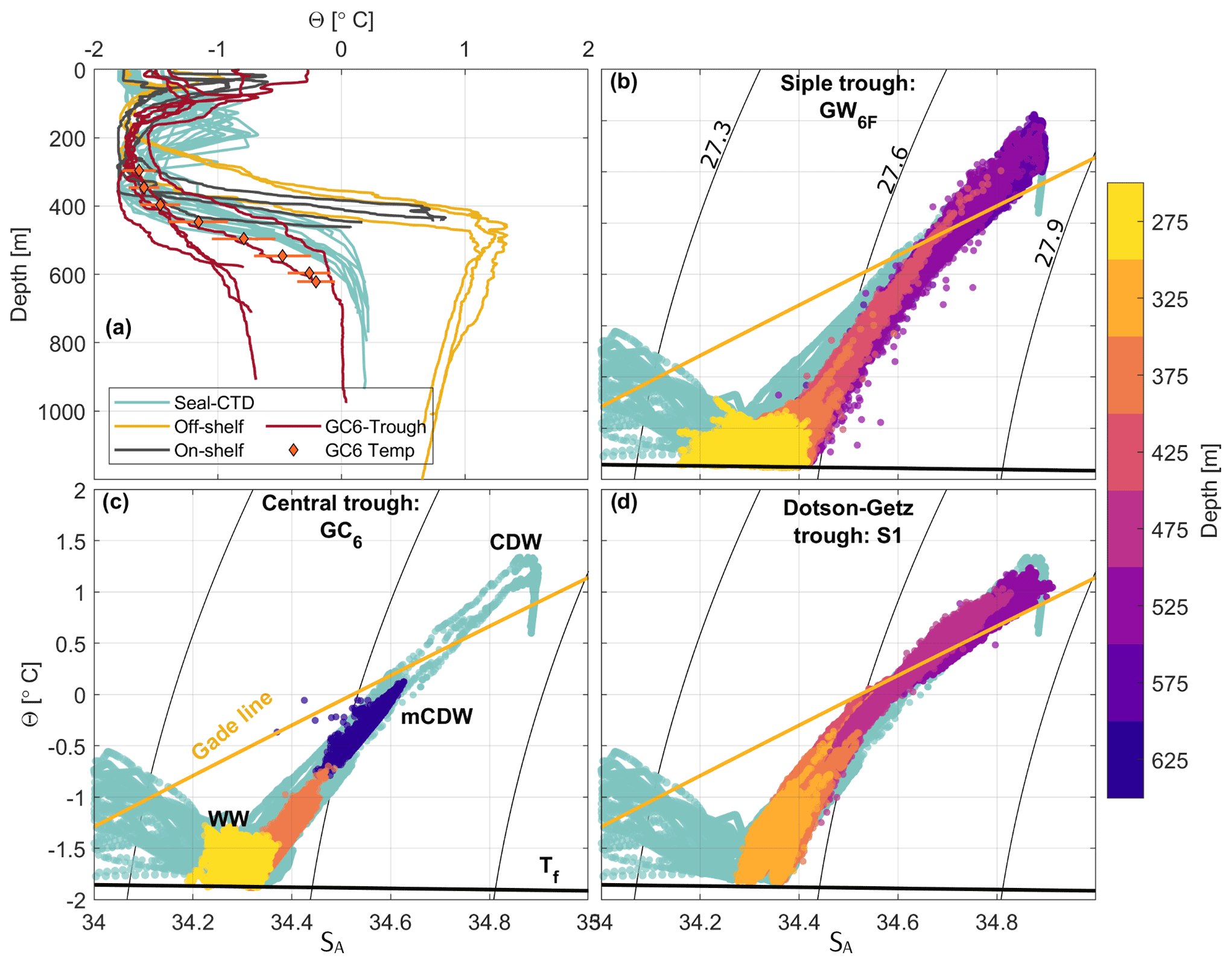
Figure 3(a) Temperature profiles taken by ship (red, black, yellow) and the seal (turquoise, see Fig. 1a, b for locations). Orange diamonds and lines show the mean temperature and standard deviation recorded by each instrument on GC6. ΘSA diagrams for (b) GW6F in the Siple trough, (c) GC6 in the GC6 Trough between Siple and Carney Islands, and (d) S1 in the Dotson–Getz Trough (see Fig. 1a for locations), color-coded by the depth of moored instruments, and with the CTD stations and seal dives from Fig. 1a marked in turquoise in the background. Four outliers are removed from S1. The σ density contours (thin black lines), the Gade line (yellow), surface freezing temperature Tf (thick black line), and characteristic water masses are labeled (WW: Winter Water, mCDW: modified Circumpolar Deep Water, CDW: Circumpolar Deep Water).
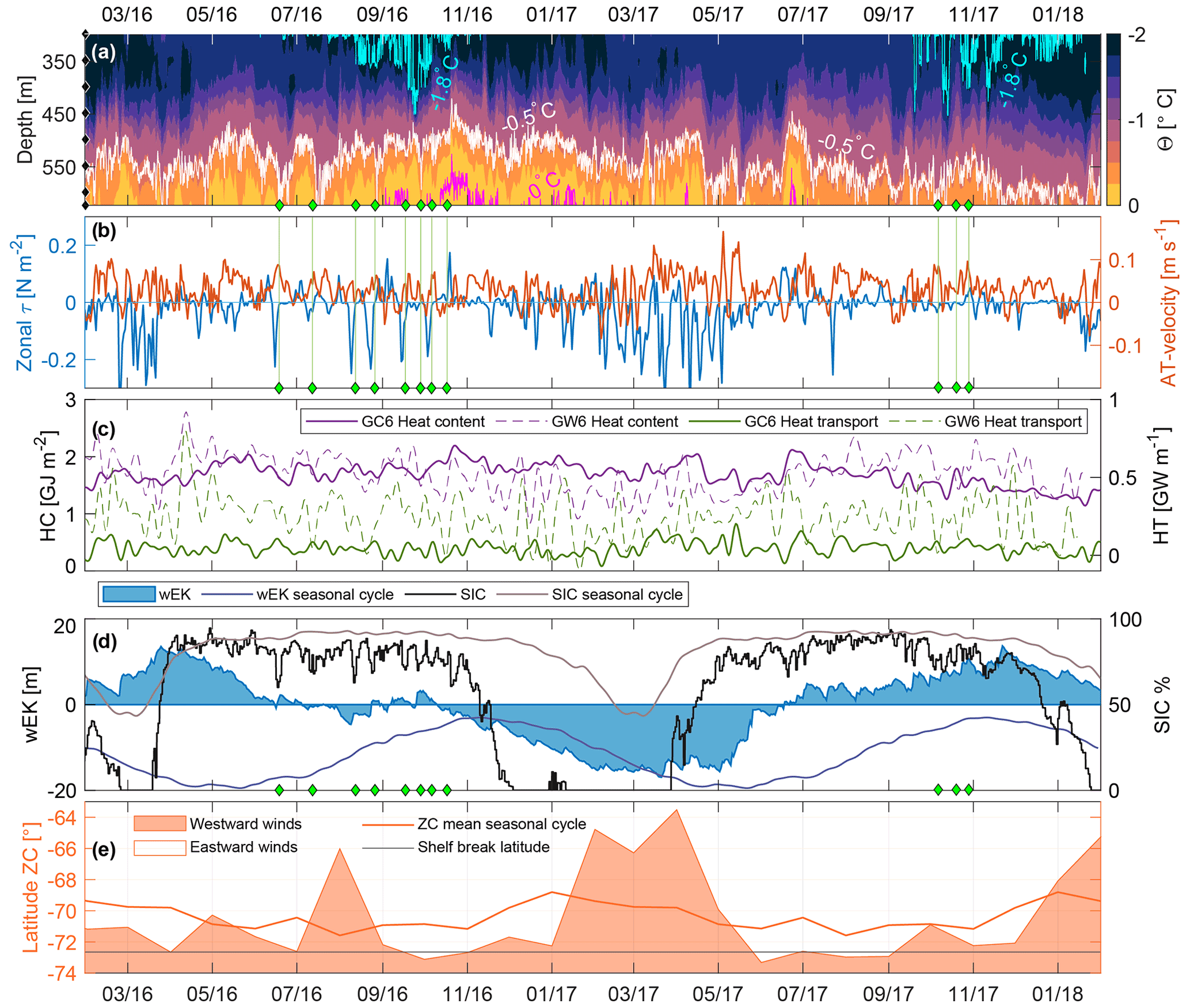
Figure 4Daily mean records from GC6 showing (a) conservative temperature, and (b) depth-averaged along-trough (AT) velocity at GC6 (red) and zonal τD18 averaged over the SB box (blue). Positive values denote flow toward the ice shelf and eastward stress respectively. The −1.8 ∘C (cyan), −0.5 ∘C (white), and 0 ∘C (magenta) contours are highlighted in (a), and the measurement depths are shown (black diamonds) in (a). (c) Heat content (HC) at GC6 (purple) and GW6 (dashed purple), and heat transport (HT) at GC6 (green) and GW6 (dashed green), all LP8D. (d) Cumulative Ekman pumping anomaly in the SB box (filled blue) and SIC over GC6 (black), with their mean seasonal cycles (2001–2018) in dark blue and gray respectively. (e) Estimated monthly mean location of the zero-contour in a meridional band spanning the zonal extent of the SB box. The filled orange area indicates westward winds and white indicates eastward winds. The thin orange and gray lines indicate the mean monthly position of the zero-contour from 2001 to 2018, and the latitude of the shelf-break north of GC6 respectively. Time is given as mm/yy. The green diamonds (a, b, d) and lines (d) mark the strong cooling events observed at GW6F (Steiger et al., 2021).
The hydrography in the ΘSA space provides information on the presence of meltwater, as the ΘSA properties will evolve along the “Gade line” when a water mass mixes with glacial meltwater. Such alignment is observed in the Dotson–Getz Trough (Fig. 3d, at Θ=0.1, SA=34.6) but neither in the Siple nor the GC6 Troughs, including the GC6 mooring, the CTD casts, and seal dives (Figs. 3b, c, 1a for CTD locations). The current's magnitude and variability are highest in the along-trough direction (Fig. 2d, solid lines) with an average velocity and standard deviation of 3±5 cm s−1. It is directed toward the ice shelf (Figs. 1a and 4b) and is nearly depth independent (barotropic) over the observed depth (407–615 m).
3.1.2 Heat content and heat transport
The average heat content relative to the in situ freezing point at GC6 is 1.7±0.2 GJ m−2. This value is lower than at the GW6-mooring in the Siple Trough even though GC6 was moored at a greater depth (650 m vs. 600 m), where the water is typically warmer. The heat content at GC6 is generally higher in 2016 than in 2017, with a maximum in October 2016 (2.4 GJ m−2) and the minimum in January 2018 (1 GJ m−2). This corresponds well with the variability of the mCWD layer, which is also thickest in October 2016 (230 m, based on the −0.5 ∘C isotherm) and thinnest at the end of the mooring time series when the entire water column is colder than −0.5 ∘C on several occasions (Fig. 4a).
The current past GC6, and hence the heat transport, is directed toward the ice shelf 78 % of the time (daily means), on average bringing 45±64 MW m−1 toward the shelf. The variability in heat transport is dominated by current variability. We, therefore, focus our following analysis on the along-trough current and temperature variability separately rather than heat transport.
3.2 Atmospheric forcing
The wind field, wEK, and SIC exhibited large differences between 2016 and 2017 (Fig. 4d, e). First, the broad eastern Amundsen Sea shelf break region was dominated by eastward winds during 2 consecutive years (2015 and 2016) since the zero-contours during the summers 2015 (not shown) and 2016 were shifted anomalously far south both north of the GC6 Trough (Fig. 4e) and over the Amundsen Sea continental shelf as a whole (not shown). Consequently, the usual period with persistent summertime westward winds did not occur. Second, wEK deviates from its typical seasonal cycle (Fig. 4d), and values are positive throughout most of mid-2015 through 2016 (Fig. 7a). Last, the summertime SIC is lower than the 2001–2018 mean over the GC6 Trough in both 2016 and 2017 (Figs. 4d and 7a, b), and 2017 stands out with 4 ice-free months. Both the surface winds and the SIC influence τ and consequently the variability of the ocean currents and temperature.
Ocean surface stress-driven variability of the along-trough current and bottom temperature at GC6
τ is an essential driver of heat content variability near several ice fronts in the Amundsen Sea. However, while τ in the continental shelf break region specifically determine heat content and heat transport in the vicinity of the ice front, where cross-cutting troughs connect the sill to the ice front (Assmann et al., 2019; Dotto et al., 2019), the heat content and transport in the GC6 Trough respond to τ over the continental shelf.
The strongest correlation between the along-trough current at GC6 and zonal τD18 occurs during winter over a region that roughly overlaps with the Amundsen Sea Polynya (ASP, Fig. 1a) and extends northward to the shelf break (Central box, Fig. 5a, , lag =0 d, BP8D–10M). The negative sign indicates that strong westward τD18 enhances the along-trough current toward the ice front. Only shorter periods of positive correlation, most notably during summer 2017, interrupt this pattern (Fig. 6b). The occurrence of periods with positive correlation is independent of the parameterization of τ (Appendix B).
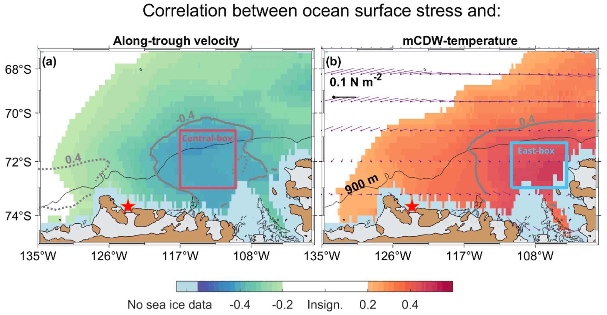
Figure 5Spatial distribution of significant correlation during winter (colors) between zonal τD18 and (a) depth-averaged along-trough velocity at GC6, and (b) mCWD temperature at GC6. The correlation calculations are based on BP8D–10M-filtered time-series averaged to daily values. Light blue regions along the coast indicate missing data on sea ice movement and white indicates insignificant correlation. Gray contours indicate a correlation of ±0.4 for winter (solid) and summer (dashed). The (a) red and (b) cyan boxes mark the areas used for average τD18 in Fig. 6. The red star and black contour mark GC6 and the 900 m isobaths respectively. In (b), the purple lines with dots at their origin indicate mean τD18 (scale in black). Values over land are removed.
For mCDW temperature, the maximum correlation with τD18 is also found during winter, but in an area further east (East box, Fig. 5b, r=0.52, lag = 4 d, BP8D–10M). The positive sign indicates that strong eastward τ correlates with higher mCDW temperatures at GC6 and holds for most of the mooring period (Fig. 6a).

Figure 6(a) τD18 (black line) averaged over the East box and mCDW temperature at the mooring site (red line). The correlation between the time series is indicated by boxes and lines: Each colored box is the center of a 100 d window (lines) with significant correlation of magnitude given by the color bar. The magenta dots show when temperatures above 0 ∘C are present. Panel (b) is analogous to (a), but for τ averaged over the Central box and along-trough (AT) velocity instead of temperature. All time series are filtered with BP8D–10M).
3.3 The regional model
From the observations, we found that the GC6 Trough is relatively cold compared with its neighboring troughs (Fig. 3), but that temperatures higher than 0 ∘C are present occasionally (Fig. 4a). Variability in the along-trough current and the mCDW temperature are both driven by τ. However, although strong currents toward the ice shelf generally correspond to westward τ over a region stretching from the ASP to the shelf break (Fig. 5a), high mCDW temperatures generally correspond to eastward stress further east on the continental shelf (Fig. 5b). We use output from the regional model to further investigate the connections between the mCDW temperature, the along-trough current, and τ, with particular attention to how the GC6 location is connected to other areas in the Amundsen Sea. First, we briefly describe hydrography and circulation in the model at the mooring site and the long-term atmospheric variability. We then look at the large-scale variability of on-shelf temperature, and finally at the overall current and temperature's relation to τERA-I.
3.3.1 The long-term state of the GC6 region
The temperature output at GC6_mod from the model over the period 2001–2017 indicates that GC6 was deployed during a relatively cold period (i.e., deep −1 ∘C isotherm, Fig. 7d). This agrees with the temperature indications from the available CTD profiles taken from ships (Fig. 3a vs. Fig. 7d). The match between the modeled and seal-borne temperature observations in 2014 are weaker: the seal-borne profiles show high bottom temperatures (Fig. 3a) and a shallow −1 ∘C isotherm, contrary to the model, which shows a strongly depressed −1 ∘C isotherm. On average, the modeled −1 ∘C isotherm at GC6_mod is found at a depth of 342±48 m (2001–2017), with roughly 200 m difference between its shallowest and deepest periods (Fig. 7c). The average depth-mean rotated velocity at GC6_mod at depths corresponding to the observed depths is 3.7±4 cm s−1 toward the ice shelf, similar to the observed average current.
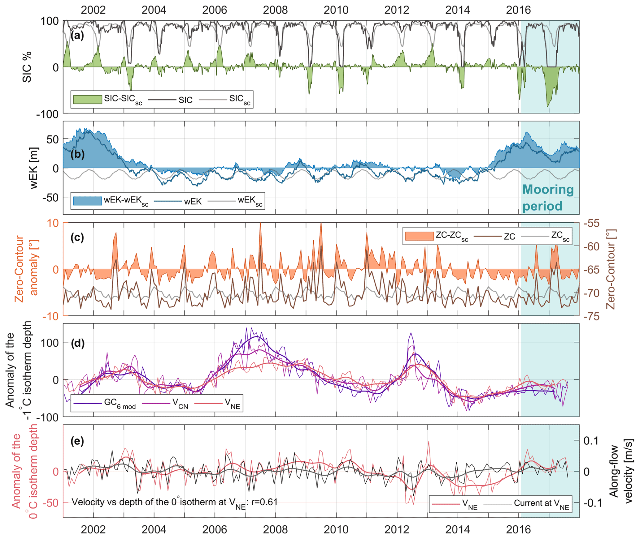
Figure 7Time-series of de-seasoned (a) SIC at GC6 (filled green), (b) cumulative Ekman pumping anomaly, wEK, (ERA 5, filled blue) averaged over the SB box (Fig. 1a), and (c) the estimated monthly mean meridional position of the zero-contour (filled orange). The subscript “SC” denotes the seasonal cycle. Light gray lines in (a)–(c) are the estimated seasonal cycles, and dark gray, dark blue and dark orange in (a)–(c) are the corresponding time-series (not de-seasoned). (d) De-seasoned modeled depth of the −1 ∘C isotherms at GC6_mod (purple), VCN (light purple), and VNE (pink). (e) De-seasoned modeled depth of the 0 ∘C isotherm (pink) and the along-flow (southeast) velocity at VNE (black). In (c), (d) thin lines are monthly means and thick lines are 12-month moving averages. In all panels, the time period with mooring measurements is marked by the turquoise background.
The SIC over the GC6 Trough, the wind field, and the wEK in the SB box display large year-to-year variability (Fig. 7a–c), with implications for the GC6 region. The wintertime SIC is always high, but highly variable between summers, ranging from ∼80 % to ice-free (Fig. 7a). There is no trend in the average wind velocity during 2001–2017, but the mooring period is within a period of relatively weak τ over the shelf break north of GC6 (not shown). Occasionally, the zero-contour does not migrate north (south) as expected during summer (winter) (Fig. 7c). wEK is generally highest at the end of winter, and lowest at the end of summer, but shows strong positive anomalies, including during the mooring period (Fig. 7a, b).
3.3.2 Long-term variability in isotherm depth
The variability in isotherm depth is important both at the shelf break for admitting warm water onto the continental shelf and on the continental shelf for the warm water's access to the base of the ice shelf. The evolution of the modeled isotherm depth anomalies (seasonal cycle removed and LP8D) follows the main flow patterns on the continental shelf, as shown in the video in the supplementary material. Anomalies of deep and shallow isotherms in the GC6 Trough seem primarily to originate from two regions: The trough northeast of GC6, which is connected to the warm waters north of the shelf break, and along the coast from regions east of Carney Island. Some anomalies travel from the eastern Amundsen Sea around Bear Ridge and continue westward along the coast (sketched arrows in Fig. 8d).
We select two locations in the regional model based on these pathways, one in the northeastern trough (VNE) and one just north of Carney Island (VCN, Fig. 8a), in order to better understand the pathways and time scales of isotherm depth anomalies traveling toward GC6. By comparing the −1 and 0 ∘C isotherm depths at VNE and VCN with GC6_mod from 2001–2017, we note three relations: First, the isotherm depth at all three locations co-varies, both on monthly and interannual timescales (Fig. 7d). Second, the low-frequency variability of the isotherm depths (12-month moving averages, Fig. 7c) responds to variations in SIC and wEK. High summertime SIC and positive wEK are favorable for a thick warm layer the following winter through weak convection and lifted isotherms. Correspondingly, low summertime SIC and negative wEK favor a thin warm layer. The thermocline depth at GC6_mod appears to be particularly sensitive to these fluctuations compared with VNE and VCN as the low-frequency variability of the −1 ∘C isotherm depth has the largest amplitude at GC6_mod (Fig. 7d). The response time to variations in SIC and wEK is up to a year owing to the slow deepening of the mixed layer after a summer of low SIC followed by sea ice formation. This response time agrees with the observed time lag from the end of the main sea ice formation period in fall to when the −1.8∘ isotherm reaches its deepest point at GC6 (Fig. 4a, d). Third, at VNE the current strength and the thickness of the warm layer correlate (r=0.61, Fig. 7e), with a strong southeastward current corresponding to a thick warm layer.
3.3.3 Regional isotherm variability
The depth of the modeled 0 ∘C isotherm averaged over 2016–2017 increases from about 200 m at the shelf break to 400 m in the GC6 Trough, and similarly from east to west (Fig. 8a), consistent with Ekman downwelling along the coast and previous observations (Jacobs et al., 2012) respectively. The main warm period in the GC6 observational records (Θ>0 ∘C: September to December 2016, Fig. 4a) lags a shallow 0 ∘C isotherm on the continental shelf by several months (Fig. 8b). Comparing summers 2016 and 2017, preceding the warm and cold winter at GC6 respectively, the isotherms in both the north-eastern trough and the Dotson–Getz Trough were shallower in 2016 than in 2017 (Fig. 8d). This delay between coherent changes on the continental shelf and at GC6 suggests that advective processes (∼3 months) bring heat to the mooring region.
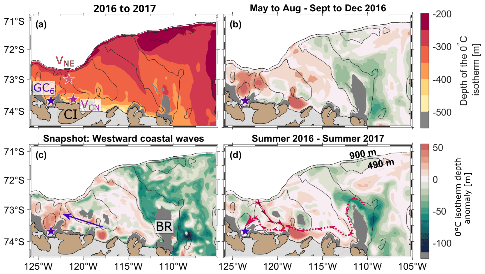
Figure 8(a) The mean depth of the 0 ∘C isotherm during 2016–2017. Carney Island (CI), Bear Ridge (BR), the virtual mooring locations VNE (pink star) and VCN (light purple star), and GC6 (dark purple) are marked in colors corresponding to Fig. 7b. (b) The difference between May to August 2016 and September to December 2016. (c) A snapshot from 8 June 2016 showing an example of wave features along the northern coast of Carney Island (seasonal cycle removed and filtered with LP8D). The blue arrow indicates the propagation direction. (d) The difference between summer 2016 and summer 2017. The red dashed arrow indicates the suggested pathways of anomalies in isotherm depth. In all panels, the black contours indicate the 900 and 490 m isobaths. The gray regions indicate that the deep 0 ∘C isotherm is not present.
The propagation time scale of the isotherm depth anomalies vary, possibly impacted by the complex interactions of anomalies from the north and east that meet north of Carney Island. The isotherm depth anomalies also reveal that eddies occasionally get “trapped” in the GC6 Trough, e.g., in June 2017, possibly contributing to sustained warm peaks (Fig. 4a). Occasionally, anomalies appear to travel as waves westward along the coast, visualized by the snapshot in Fig. 8c.
3.3.4 Spatial correlation of ocean surface stress with ocean currents and temperature
From the observations, we identified that the currents at GC6 correlate best with τD18 over the Central box, whereas the mCDW temperature at GC6 correlates best with τD18 over the Eastern box. Here, we study the correlation of τERA-I over these two areas with the modeled currents and temperatures in the surrounding areas on the continental shelf (Fig. 9). We separate between the deep (below the 0∘ isotherm) and the shallow (above 100 m depth) layers to distinguish between the deep-reaching and shallow effect of τ on currents and temperature. The overall correlation between τ and currents and temperature is strongest during winter, in agreement with results from GC6 (Fig. 5), and we, therefore, focus this section on winter conditions. Comparing the 2 years of observations, the model generally shows a more significant and stronger correlation in 2016 than in 2017 (not shown), making 2016 similar to the winter average, as suggested by the observations.
Regions of strong currents generally have a significant correlation with τ over the Central box (Fig. 9c, d). The deep currents have a strong positive correlation over the eastern flanks of the Dotson–Getz and the northeastern Troughs, and along the shelf break toward the entrance of the Dotson–Getz Trough. This means that eastward (positive) τ enhances the currents toward the ice shelf and eastward along the continental shelf break, i.e., in the mean flow direction (positive current anomaly).
At the GC6 location, the positive correlation of τ over the Central box with modeled currents disagrees with the negative correlation with the observed current. As the model's representation of the current's short-term variability at GC6 is unreliable and its local bathymetry is inaccurate, this is not surprising.
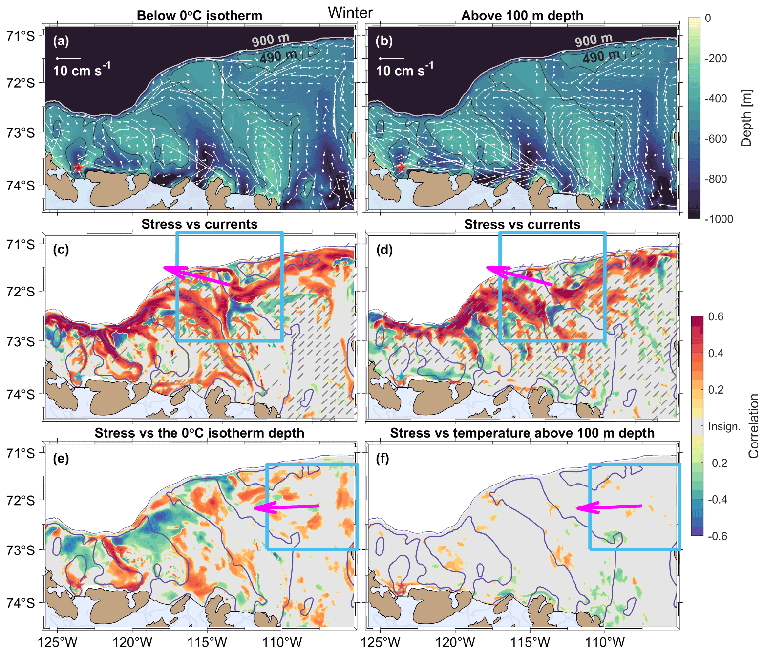
Figure 9(a, b) Bathymetry (color) and mean modeled currents (white sticks, 2016 to mid-2017) at every 7th regional model grid point during winter (a) below the 0 ∘C isotherm, and (b) above a depth of 100 m. The current scale is indicated in the top left corner, and the current is directed from the white circle indicating the grid cell center. Currents weaker than 1 cm s−1 are omitted. The red star indicates GC6. (c, d) Maps of correlation between modeled currents and the zonal τERA-I averaged over the Central box (cyan) (c) below the 0 ∘C isotherm and (d) above a depth of 100 m. Gray regions have an insignificant correlation, and the white region is outside the on-shelf study domain. Hatched regions have mean currents less than 1 cm s−1. Panels (e) and (f) are analogous to panels (c), (d), but show correlation between the zonal τERA-I averaged over the East box (cyan) and (e) the depth of the 0 ∘C isotherm, and (f) temperature above a depth of 100 m. The contours shown are the 900 m (thin blue line) and 490 m (thick blue line) isobaths. The magenta arrow shows the direction of the mean τERA-I over the boxes. In (c), (d), (e), (f) all time series are de-seasoned and LP8D is applied, and the color of the star shows the correlation between τERA 5 and the along-trough current (c, d) and mCDW temperature (e, f) from Fig. 5.
The shallow currents (above 100 m) also have a positive correlation along the shelf break north of GC6 and partly into the Dotson–Getz Trough, comparable with the deep currents but slightly weaker. This indicates that eastward τERA-I induces a positive anomaly in the mean current direction throughout the water column in these regions, except for the coast north of Carney Island. There, a negative correlation indicates that westward (negative) τERA-I enhances the westward current (positive, owing to the local rotation of the coordinate system with the mean current direction). In the regions of high correlation, the lag between τERA-I and the surface currents and deep currents is 0–1 d and 1–2 d respectively.
Similar to the correlation of the deep currents with τERA-I, the 0 ∘C isotherm depth has a strong positive correlation with τERA-I within the northeastern trough (Fig. 9e). Eastward τERA-I consequently induces both a shoaling of the 0 ∘C isotherm depth and a strengthened southeastward current there. This indicates that the long-term result of correlation between current and isotherm variability from VNE holds for the entire northeastern trough. At GC6 the correlation is also positive, in agreement with observations. As expected, above a depth of 100 m the correlation with temperature is mostly insignificant, which emphasizes that τERA-I influence the ocean temperature mostly through deep-reaching dynamic processes.
Based on the correlation maps from the model output, we suggest that the wind stress over the Central box induces variability in the continental shelf break regions of strong currents during winter, i.e., within the troughs leading to the ice shelves, but that the correlation at the GC6 mooring is not well captured by the model. The impact of the wind stress on temperature is greatest for the deep isotherm depth, with less impact on the temperatures of the upper water column.
4.1 Differences from the Siple and Dotson–Getz Troughs
The hydrographic conditions at GC6 highlight the importance of bathymetry: despite the geographic proximity to the Siple and Dotson–Getz Troughs, the hydrography differs greatly (Fig. 3 and Assmann et al., 2019; Wåhlin et al., 2013). The variability has been observed in snapshot CTD profiles reported in Jacobs et al. (2013). There are three fundamental hydrographic differences: (i) The maximum temperature observed in the GC6 Trough is lower (0.19 ∘C, 2014, seal-borne CTD, Fig. 3a) than in the adjacent troughs, i.e., pure CDW is absent. Since GC6 records temperatures above 0 ∘C and is moored on the slope of the trough, unmodified CDW could be present, but unobserved, in the deepest parts of the trough. However, the historical profiles record weak temperature gradients below the thermocline (Fig. 3a) so that the mooring is likely representative for temperatures at depth. (ii) mCDW influenced by meltwater is not observed in the GC6- and Siple Troughs, but is registered in the Dotson–Getz Trough (Wåhlin et al., 2010). Although the Dotson–Getz Trough sill depth is ∼70 m shallower than the Siple Trough sill, the shallower isotherms north and east on the continental shelf enable basal melt. We note that although meltwater is unobserved in the GC6 Trough, the heat available could still induce basal melt without this being detected. The available data are insufficient to assess whether meltwater, e.g., exits at shallow depths or through pathways underneath the ice shelf. (iii) Seasonality in deep currents and isotherms is absent in the GC6 and Siple Troughs in 2016–2018, but is present in the Dotson–Getz Trough (Wåhlin et al., 2013). Further south in the Dotson–Getz Trough the seasonality disappears (Jacobs et al., 2012), possibly because of mixing by internal waves and basin-scale eddies (Wåhlin et al., 2013).
The mean current at GC6 brings an estimated 45±64 MW m−1 available heat toward the GIS front south in the GC6 Trough, about one fifth of the values observed in the Siple Trough (GW6). The heat transport at GC6 might nonetheless be important for the central GIS: The current in the Dotson–Getz Trough is even weaker, and the heat transport conveyed toward the Dotson Ice Shelf is roughly half the value observed at GC6 (Wåhlin et al., 2013), and still, meltwater is observed here (Wåhlin et al., 2010). Estimates of heat transport based on single moorings, however, come with uncertainties related to capturing the width of the current and depends on the position of the core of the warm inflow relative to the mooring location. Estimates based on mooring arrays across the troughs would yield more reliable comparisons.
4.2 Correlation between the along-trough current and τ
The heat transport at GC6 is dominated by the variability in the along-trough current, as previously observed in the Dotson–Getz Trough (Wåhlin et al., 2013) and further east in the trough at 113∘ W (Assmann et al., 2013). The along-trough current's dominant response to τ, however, differs from results from troughs both west and east of the GC6 Trough: the strong westward τ over the continental shelf between the ASP and the shelf break corresponds to a strong current toward the ice shelf (BP8D–10M, Figs. 5a and 9b). There, the strongest currents toward the ice front are driven by eastward τ just north of the shelf break (Wåhlin et al., 2013; Assmann et al., 2013). This suggests that τ directly adjusts the barotropic component of the along-shelf currents, and consequently the direct flow of the undercurrent into these adjacent, deep troughs, whereas a different mechanism is responsible for the co-variability at GC6. The lag of 0–2 d between τ and the along-trough current at GC6 is, however, close to results from a similar correlation analysis from other regions (Darelius et al., 2016; Wåhlin et al., 2013).
The location of the highest correlation between τ and the along-trough current (Fig. 5a) indicates that the wintertime link between τ and the along-trough current is related to ASP-specific features, such as the low wintertime SIC, the consistently strong winds that facilitate rapid momentum transfer from the atmosphere to the ocean, and its location over the coastal current. Without this polynya region of reduced SIC, which occasionally extends northward toward the shelf break, and the disturbance of potential fast-ice, the wintertime relation between wind and current would possibly be much reduced. This suggests that current variability at GC6 is connected to τ-induced variability propagating with the coastal current. We speculate that the response might be largely barotropic. Westward winds increase the along-shore sea level and enhance the westward barotropic current along the coast, affecting the variability at GC6. This process would induce a negative correlation between the ocean surface stress and current at GC6, which is what we observe in winter. The nonsignificant correlation between τERA-I and the coastal current (Fig. 9c), which contradicts this hypothesis, might result from the complex coastal geometry and bathymetry, large cyclonic systems, changes in the density structure which affect the balance between the barotropic and baroclinic components (Núñez-Riboni and Fahrbach, 2009; Kim et al., 2016), varying propagation speed of anomalies, irregular wave patterns along the coast, and trapped warm and cold anomalies. The variability in transport within the coastal current is also connected to the amount of meltwater produced from basal melt in ice shelf cavities (Nakayama et al., 2014a; Jourdain et al., 2017). We also note that the error in the estimation of τ introduced by assuming a motionless ocean might influence results in this region where the surface currents are strong.
In summer, the relationship between τ and the current at GC6 shifts: the correlation turns positive, and the region of highest correlation shifts west of Siple Island (dashed contour in Fig. 5a). The temporal and spatial changes in correlation are unlikely explained by momentum transfer from sea ice, given the insensitivity of the correlation results to the different sea ice parameterizations for τ (Appendix B). However, the indirect effect of sea ice on the dynamics through, for example, stratification, might be of importance.
4.3 Variability in heat content
Periods of increased temperatures at GC6 are likely the result of at least two mechanisms. One is a short-term response where eastward τ is associated with short-term Ekman upwelling and local lifting of the thermocline. The second is a long-term response where positive cumulative Ekman pumping anomaly (wEK), high summertime SIC, and remote input of heat from the eastern Amundsen Sea and the deep ocean north of GC6 adjust the isotherms by up to 200 m (Fig. 7b). The two responses are distinguished by causing short (less than 3 weeks) and long (several months) periods of increased heat content at GC6.
The positive correlation between mCDW temperature and τD18 over the eastern shelf in winter (BP8D–10M, Fig. 5b) is associated with the short-term response, similar to observations in the Siple Trough, but different than the Dotson–Getz Trough where the high bottom temperatures are less related to the average wind over the shelf break (Wåhlin et al., 2013). This indicates that the bottom temperatures in the western Amundsen Sea are more sensitive to changing wind forcing than those in the eastern Amundsen Sea, which is supported by a higher standard deviation in isotherm depth west of the northeastern trough in the regional model (not shown). The time scale of the short-term response is similar to that under the Pine Island Ice Shelf (Davis et al., 2018).
During summer, the correlation is mostly insignificant, but shows signs of anti-correlation (Fig. 6a). We speculate that the insignificance is due to this shift from positive to negative correlation but that the shift happens too gradually for our moving windows to capture periods of significant negative correlation. We further suggest that the shift depends on the position of the zero-contour, as we observe that a northward shifted zero-contour coincides with periods of anti-correlation between the zonal stress and the mCDW temperature. Dominating westward winds, general depression of the thermocline at the shelf break, and increased summer stratification also likely weaken the relationship between τ and the deep temperatures.
The cooling events at GC6, which are similar to those observed at GW6F during the same period (Steiger et al., 2021), might be triggered by strong winds over a region of low SIC east of Carney Island. The estimated propagation speed of a coastal trapped wave from this region to GC6 (0.4–0.7 m s−1) matches the propagation speed of the coastal trapped wave observed at GW6F (Steiger et al., 2021). The effect of the events on the heat content at GC6 is less than at GW6F, possibly explained by the larger distance of GC6 from the ice shelf front. However, this implies that the signal is stronger at the ice shelf front than at GC6. Consequently, the effect of this wind-induced coastal wave is likely substantial at the ice shelf front in the GC6 Trough.
The difference in heat content between 2016 and 2017 and the multi-yearly variability indicated by the model emphasizes the importance of the different atmospheric forcing between 2016 and 2017 specifically and the influence of the long-term response in general. The two consecutive years (2015 and 2016) of southward shifted zero-contours might have induced the large positive wEK anomaly in 2016, possibly leading to shallower isotherms during summer 2016 than in 2017 in both the coastal region and the northeastern trough (Fig. 8d). In 2017, the reduced wEK and strong thermohaline convection during freeze-up following the exceptionally low SIC might have caused the prolonged presence of WW below a depth of 300 m and deep isotherms relative to 2016 (Fig. 4a). However, according to the long-term model results, both 2016 and 2017 were relatively cold, despite the strong positive anomaly in wEK (Fig. 7a). The absence of an evident relation between wEK and heat content such as observed in the Siple Trough (Assmann et al., 2019) indicates that the low summertime SIC, as well as other large-scale atmospheric forcing mechanisms not assessed here, is more central for heat content variability at GC6 than wEK.
Several additional processes beyond the scope of this study govern shelf break regions. Passing coastally trapped waves (Chavanne et al., 2010) and the surface water thickness and composition (Daae et al., 2017) might affect the undercurrent's strength and depth. The undercurrent can further induce vortex systems and Rossby waves along the shelf break, bringing heat into troughs (St-Laurent et al., 2013). In the regional model, waves appear in the 0 ∘C isotherm along most of the Amundsen Sea shelf break but dissolve in the region north of GC6, suggesting a minor influence on the heat content variability at GC6. We also note that the connection between increased basal melt from ice shelf cavities and the transport of the coastal current (Jourdain et al., 2017) might contribute to the variability we observe in the GC6 Trough, and that strong anomalies in heat loss in upstream polynyas, such as the ASP, can cause reduced heat content for several years (St-Laurent et al., 2015).
4.4 Large-scale climate variability
Jacobs et al. (2013) suggested that the Amundsen Sea responds to large-scale changes as a unit, and consequently, the long-term variability at GC6 could be influenced by far-field drivers such as the El Niño southern oscillation (ENSO) and anomalies in the Southern Annular Mode (SAM) (Dutrieux et al., 2014; Thompson et al., 2018; Spence et al., 2014).
The future changes in ENSO are disputed (e.g., Perry et al., 2020), however, the SAM index has a positive trend (a southward shifting zero-contour) owing to CO2 emissions and ozone depletion (e.g., Swart and Fyfe, 2012; Thompson and Solomon, 2002; McLandress et al., 2011). This might lead to reduced Ekman transport toward the coast, a relaxed ASF, and a combination of westward stress on the continental shelf and eastward stress along the shelf break, favoring increased heat transport toward the ice front at GC6 and increased mCDW-layer thickness respectively. Although a clear relationship between the SAM index and wEK and isotherm depth is absent on monthly time scales (not shown), the long-term trend might drive a slow change in the region. SIC also tends to be high during the positive mode of SAM (Lefebvre and Goosse, 2005), and indications of this occur over GC6. The future state of SIC might be particularly important for the GC6 Trough as isotherm deepening due to sea ice growth seems to have a larger impact here than elsewhere in the Amundsen Sea (Fig. 7c).
In the long term, the expected positive trend in SAM might influence the heat content at GC6 owing to the link to atmospheric forcing. A permanently relaxed ASF would likely weaken the undercurrent and possibly enhance the relative importance of the wind-driven heat input from the east. However, the short-term relationship between τ and the bottom temperatures could be reduced by increased surface stratification due to increased sea ice melt. Still, the impact of future changes in SIC is uncertain given its contradicting response to positive SAM (Lefebvre and Goosse, 2005) and a warmer atmosphere. The shift in τ associated with the trend in SAM would not affect the katabatic winds, and thus the relation between τ and heat transport at GC6 might be unchanged.
This study provides a first detailed description of the hydrography and ocean circulation close to the front of the GIS between Siple and Carney Islands and its response to atmospheric forcing using new mooring observations (GC6) combined with output from a regional model (Nakayama et al., 2018, 2019) and historical CTD profiles. The mooring data show temperatures over C throughout the mooring period and recurring periods with temperatures over 0∘C (Fig. 4a). The average heat transport is directed toward the ice shelf (Fig. 2d), but contrary to adjacent fronts (Assmann et al., 2019; Wåhlin et al., 2013), unmodified Circumpolar Deep Water (CDW) is absent (Fig. 3c). The data show no modification of CDW at depth by basal melt in the GC6 Trough (Fig. 3c) as observed in the neighboring Dotson–Getz Trough (Wåhlin et al., 2010).
We analyzed the atmospheric drivers of the mesoscale (8 d to 10 months) variability in the deep, warm temperatures and circulation at GC6 and found a link to ocean surface stress (τ, Figs. 5 and 6). In winter, strong eastward τ over the eastern shelf break increases mCDW temperatures, whereas strong westward τ over the Amundsen Sea Polynya region and northward to the continental shelf break (Central-box) strengthens the along-trough current. These relations agree with (i) short-term relaxing of the Antarctic Slope Front (ASF), lifting of the thermocline and an accelerated undercurrent, and (ii) piling up of water along the coast and a strong westward barotropic current. Barotropic responses along the path of the coastal current may thus partly explain the high correlation and short lag between τ over the Central box and the along-trough current at GC6. However, the analyzed model fields do not confirm this. The opposite sign of correlation of τ with the current and mCDW temperature emphasize that advection of heat by the southward current is not the primary driver of temperature variability at the mooring on these time scales. The temperature response to τ is similar in the GC6 and Siple Troughs, whereas the response of the currents differs between the GC6 Trough and the Siple and Dotson–Getz Troughs, emphasizing the importance of bathymetry.
The link between heat content, heat transport, and τ changes in summer – there is a shift in the dynamics induced by τ that is likely connected to stronger stratification and higher baroclinicity.
Winter conditions appear to favor wind-driven enhanced heat content near the ice front (Fig. 6a). In winter, the wind field's zero-contour generally shifts southward, which we find facilitates a warm GC6 Trough. The positive wEK is also generally strongest in winter (Fig. 7b), in agreement with a suggested weakened ASF in mid-winter (Pauthenet et al., 2021). Uncharacteristic atmospheric forcing during the mooring period (Fig. 7a, b) likely explains the lack of seasonality in the GC6 mooring record. Mixing by internal waves and basin-scale eddies might contribute, such as south in the Dotson–Getz trough (Wåhlin et al., 2013). The warm 2016 was characterized by winter-like forcing, whereas the colder 2017 tended toward forcing more typical for summer (Fig. 4d, e). Compared with the long-term model results, however, the winter-like 2016 was not particularly warm (Fig. 7c). This emphasizes the complex interactions of forcing mechanisms, and strong positive wEK and a southward shifted zero-contour can be hindered from causing anomalously shallow isotherms on the continental shelf by counteracting forcing mechanisms such as low summertime SIC.
We conclude that although the entrance to the GC6 Trough is sheltered from warm water inflow by bathymetry, it is connected to atmospheric forcing and conditions elsewhere on the continental shelf. This makes the ice front in the GC6 Trough vulnerable to future changes in the wind field, SIC, and thermocline characteristics, just like the other ice fronts of the GIS. Sensitivity studies with a numerical model as well as improved bathymetry data at the fronts and under the ice shelf could provide further knowledge on how higher temperatures and a shallower thermocline at GC6 might affect meltwater production and the stability of the GIS. This would help to assess its contribution to future freshwater input toward the Ross Sea and how this could affect large-scale aspects such as the thermohaline circulation.
For the virtual mooring GC6 mod, we choose a location on the model grid slightly southwest of the actual mooring site as the depth at this location is similar to the mooring depth. Trough openings are generally deeper and less restricted in the regional model bathymetry than in the IBCSO dataset. The entrance to the trough at the shelf break northeast of GC6 is shallower than 490 m in the IBCSO, closing off the connection to the open ocean, whereas the sill is deeper in the model bathymetry (Fig. A1a). The IBCSO is expected to perform well in shelf break regions, and such features may thus help explain differences between model and observations.
Like similar models, such as the MITgcm setup used by Assmann et al. (2013), this regional model reports bottom temperatures that are too high and a warm layer that is too thick. In agreement with observations, however, CDW is not present at GC6. Also, seasonality is imposed on the thinning (summer) and thickening (winter) of the warm layer that is not detected by GC6. As the warm layer extends higher up in the water column in the model (a difference of about 100 m), the interaction between cool surface waters through deep ventilation and the warm layer seems to be more important in the model than in observations. Applying BP8D–10M to the −1 ∘C isotherm, however, yields relatively good agreement between the model and observations (r=0.31, Fig. A1b). Although the model does not resolve observed sudden changes in temperature as we observe in, for example, May 2017, and imposes a few artificial peaks (Fig. A1b), the Fourier spectra support the conclusion that the magnitude of variability is relatively good, in both the upper and the lower layers of mooring extent (Fig. A1c).
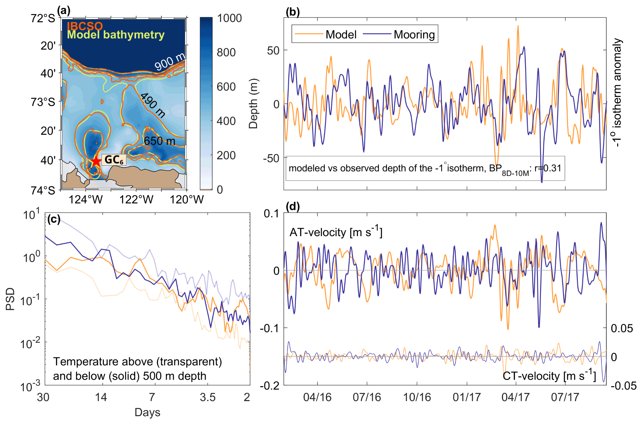
Figure A1Comparison between (a) selected isobaths from the IBCSO (orange) and the model's bathymetry (yellow) (GC6's location: red star). 650 m is the mooring depth and at 490 m the model bathymetry indicates that the trough northeast of GC6 is open, whereas it is closed in the IBCSO data. (b) The anomaly of the −1∘C isotherm depth, (c) the Fourier spectra of mean temperature above (transparent) and below (solid) a depth of 500 m, and the (d) rotated along-trough current (AT velocity, left axis) and cross-trough current (CT velocity, right axis) at the mooring of GC6 (blue) and at the mooring location in the model (orange). Isotherm depth anomalies and rotated velocities are filtered with BP8D–10M.
Velocity variance ellipses from observations and model at the mooring location are similar in both magnitude and variability, and in variation with depth (Fig. 2d). This is true both for the model period as a whole and during most of the period when separated into monthly mean variance ellipsis. This indicates good agreement on the overall background state. The main difference is in the magnitude of the zonal component, which tends to be of the opposite sign, but as this is the minor component in both the model and observations, it is largely disregarded through rotation of the coordinate system along the direction of the mean flow (Fig. A1e). This slight difference in direction might be explained by differences in model and true bathymetry (Fig. A1a). Frequency spectra of velocity also indicate that the relative importance of variability on various time scales agrees well (not shown), and the depth profiles of decomposed principal components through EOF analysis are similar, although the model overemphasizes PC1. The variability explained by the main components, PC1, and PC2, varies with time and co-vary for model and observations. These aspects all yield credibility to the use of the regional model to describe the average situation in the GC6 Trough region on longer time scales.
There is, however, less agreement in velocity on shorter time scales (Fig. A1e). The velocity is represented well during specific periods (e.g., February–April 2017) and nearly opposite during other periods (e.g., November and December 2016). For this reason, we do not rely on the short-term variability of the modeled velocity at the mooring site.
Just like in the daily model record, the monthly mean time-series (2001–2017) exhibit strong seasonality in temperature and salinity. The warm and saline layer at the bottom is thinner in summer than in winter – in summer, the previous winter's deep ventilation pushes the deep layer of mCDW downward. However, although ventilation of cool surface waters appears to affect and interact with the deep warm layer (Sect. 3.3.2), the model appears to underestimate the extent of the deep ventilation. WW is never present below a depth of 200 m (the depth comparable with 300 m in the observations). In contrast, the mooring captures water below −1.8 ∘C down to 450 m depth. Low salinity levels compared with the observations throughout the model period indicate that the brine release due to sea ice formation in fall is under-estimated in the model. This would explain the shallow extent of deep ventilation. The slope of the mixing line between WW and CDW in yearly mean TS diagrams does, however, increase (decrease) in league with decreasing (increasing) SIC (not shown). Extensive freeze-up after periods of low SIC means deep ventilation of more saline waters, shifting the slope in the TS diagrams.
The depth of the modeled 0 ∘C isotherm averaged over 2016–2017 increases from about 200 m at the shelf break to 400 m north of GC6. There is a similar increase from east to west (Fig. 8a), which agrees with observations from Jacobs et al. (2012). In the troughs, the isotherm stays shallow further onto the continental shelf.
For calculations that include τ, we select three spatial boxes: one at the shelf break just north of GC6, the “SB box”, one over the Amundsen Sea Polynya and north to the shelf break, the “Central box” (see colored rectangles in Fig. 1a), and one on the continental shelf further east, the “East box”. The first was chosen to explore if the shelf break processes are equally important at GC6 as at GW6–7 further west (Assmann et al., 2019), and for estimations of wEK and the meridional position of the zero-contour. The Central box was chosen, because we find the highest correlation between τD18 and the along-trough current at GC6 over the ASP region and northward to the shelf break (see Sect. 3.2). The East box was chosen based on the region of highest correlation between τD18 and the mCDW temperature at GC6. We define the cumulative Ekman pumping anomaly (wEK) as the de-trended integral of wEK in time. dt is the time between observations and
In this approximation, the dependency on is neglected as the main gradients in τ are in the meridional direction, and is neglected, since f is constant in longitude.
We include SIC and sea ice movement in the approximation of τ to account for the drag of ice on the ocean following Dotto et al. (2018):
where α is SIC, is the drag coefficient between ice and water, Uice is the velocity of the ice, ρair=1.25 kg m−3 is the density of air, is the drag coefficient between air and water, and Uair is the 10 m wind. Comparison of four different estimates of τ using (i) output from ERA 5, (ii) Eq. (B2a) (Dotto et al., 2018), (iii) Eq. (B2c) with Cd parameterized using SIC (Andreas et al., 2010), and (iv) Eq. (B2c) (only wind stress) shows that inclusion of sea ice reduces the magnitude, but the variability is similar between all four estimations (Fig. B1). We do, however, assume a motionless ocean and a spatially and temporally constant Cd, although it would be more accurate to use the relative velocities between air, sea ice, and ocean, and Cd as a function of variables such as roughness, seasons, and geometry (Brenner et al., 2021). We choose to use Eq. (B2a) because previous studies have shown that the inclusion of sea ice and sea ice movement is important for a realistic estimate of momentum transfer into the ocean (Dotto et al., 2018), and do not have daily data on surface currents available for the full study period.
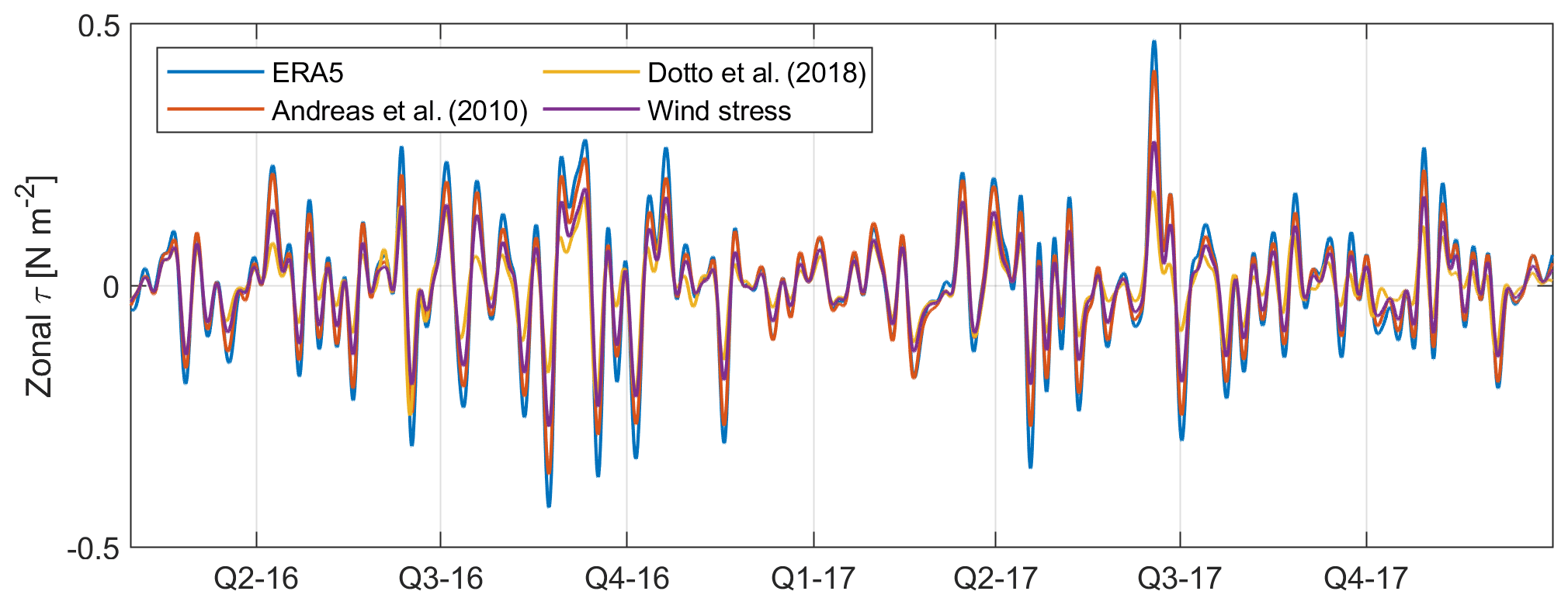
Figure B1Different estimations of τ using the output from ERA 5 (blue), and explicit calculations using the parameterization of Cd from Andreas et al. (2010) (red), parameterization of Cd from Dotto et al. (2018) (yellow), and the wind stress without accounting for sea ice (purple). All time series are filtered with BP8D–10M.
τ over the ASP region appears to be particularly influential on the currents, compared with the rest of the Amundsen Sea area: High correlation occurs in a region similar to the ASP on a correlation map between spatially varying τ and the current at a fixed location at the shelf break where the correlation is high in Fig. 9c. The temporal evolution of correlation between heat transport and τD18 is similar for stress averaged over the ASP and shelf break regions (SB box), indicating that the large-scale wind field induces the dominant current variability at GC6. Similarly, the four different parameterizations of sea ice for τ (Fig. B1) give similar temporal and spatial variability, but the magnitude of correlation increases with parameterizations including sea ice concentration and drift.
Data from moorings GC6 and GW6 are available through the NMDC data center (https://doi.org/10.21335/NMDC-1721053841, Darelius et al., 2018; https://doi.org/10.21335/NMDC-518522938, Darelius et al., 2022). Data from moorings GW6F and S1 are available through NCEI at https://doi.org/10.25921/6pwp-1791 (Wåhlin et al., 2019) and https://www.ncei.noaa.gov/archive/accession/0211128 (Wåhlin et al., 2020b). The CTD data from tagged seals are available at https://www.meop.net/ (last access: September 2019), and the ship-based CTD data taken onboard N.B. Palmer are available through the World Ocean Data Base (https://doi.org/10.3334/cdiac/otg.clivar_ross_sea_320619940214, Jacobs et al., 2014a; https://doi.org/10.3334/cdiac/otg.clivar_ross_sea_320620000215, Jacobs et al., 2014b; https://doi.org/10.3334/cdiac/otg.320620070203, Jacobs et al., 2016) and from Araon through KPDC (https://doi.org/10.22663/KOPRI-KPDC-00000634.2, Kim, 2016; https://doi.org/10.22663/KOPRI-KPDC-00000907.1, Kim, 2018) upon request. The daily model output is available at https://ecco.jpl.nasa.gov/drive/files/ECCO2/LLC1080_REG_ 10 AMS/1080_run260_2016_2018_daily (Nakayama et al., 2019), and the monthly model output at https://ecco.jpl.nasa.gov/drive/files/ECCO2/LLC1080_REG_ AMS/run260/ (Nakayama et al., 2018); new users must register for an Earthdata account at https://urs.earthdata.nasa.gov/users/new to access these files. The MEOP data set is available after filling in a form that is available at https://www.meop.net/database/download-the-data.html (see Treasure et al., 2017 and Roquet et al., 2013, 2014 for further information).
The supplementary Video S1 can be accessed at https://doi.org/10.5446/56380 (Dundas et al., 2022).
VD wrote the first draft, conducted analysis, and prepared the figures. ED processed the data. ED, KD, and NS improved the manuscript. YN provided output from the regional model. ED and TWK contributed to the field work. All authors read and commented on the paper.
The contact author has declared that none of the authors has any competing interests.
Publisher’s note: Copernicus Publications remains neutral with regard to jurisdictional claims in published maps and institutional affiliations.
The authors would like to thank Ilker Fer from the Geophysical Institute, University of Bergen, for comments on the manuscript and for lending instrumentation for CG6. The authors also thank two anonymous reviewers for constructive comments, which helped to improve the manuscript. The marine mammal data were collected and made freely available by the International MEOP Consortium and the national programs that contribute to it (http://www.meop.net).
This research is supported by the Norwegian Research Council (grant no. 267660 (TOBACO)) and the Korea Polar Research Institute (grant no. PE2211).
This paper was edited by Karen J. Heywood and reviewed by two anonymous referees.
Andreas, E. L., Horst, T. W., Grachev, A. A., Persson, P. O. G., Fairall, C. W., Guest, P. S., and Jordan, R. E.: Parametrizing turbulent exchange over summer sea ice and the marginal ice zone, Q. J. Roy. Meteor. Soc., 136, 927–943, https://doi.org/10.1002/qj.618, 2010. a, b
Arndt, J. E., Schenke, H. W., Jakobsson, M., Nitsche, F. O., Buys, G., Goleby, B., Rebesco, M., Bohoyo, F., Hong, J., Black, J., Greku, R., Udintsev, G., Barrios, F., Reynoso-Peralta, W., Taisei, M., and Wigley, R.: The International Bathymetric Chart of the Southern Ocean (IBCSO) Version 1.0 – A new bathymetric compilation covering circum-Antarctic waters, Geophys. Res. Lett., 40, 3111–3117, https://doi.org/10.1002/grl.50413, 2013. a, b
Arneborg, L., Wåhlin, A. K., Björk, G., Liljebladh, B., and Orsi, A. H.: Persistent inflow of warm water onto the central Amundsen shelf, Nat. Geosci., 5, 876–880, https://doi.org/10.1038/ngeo1644, 2012. a
Assmann, K. M., Jenkins, A., Shoosmith, D. R., Walker, D. P., Jacobs, S. S., and Nicholls, K. W.: Variability of Circumpolar Deep Water transport onto the Amundsen Sea continental shelf through a shelf break trough, J. Geophys. Res.-Oceans, 118, 6603–6620, https://doi.org/10.1002/2013JC008871, 2013. a, b, c, d, e, f
Assmann, K. M., Darelius, E., Wåhlin, A. K., Kim, T. W., and Lee, S. H.: Warm Circumpolar Deep Water at the Western Getz Ice Shelf Front, Antarctica, Geophys. Res. Lett., 46, 870–878, https://doi.org/10.1029/2018GL081354, 2019. a, b, c, d, e, f, g, h, i
Brenner, S., Rainville, L., Thomson, J., Cole, S., and Lee, C.: Comparing Observations and Parameterizations of Ice-Ocean Drag Through an Annual Cycle Across the Beaufort Sea, J. Geophys. Res.-Oceans, 126, e2020JC016977, https://doi.org/10.1029/2020JC016977, 2021. a
Chavanne, C. P., Heywood, K. J., Nicholls, K. W., and Fer, I.: Observations of the Antarctic Slope undercurrent in the Southeastern Weddell Sea, Geophys. Res. Lett., 37, 3–7, https://doi.org/10.1029/2010GL043603, 2010. a, b
Daae, K., Hattermann, T., Darelius, E., and Fer, I.: On the effect of topography and wind on warm water inflow—An idealized study of the southern Weddell Sea continental shelf system, J. Geophys. Res.-Oceans, 122, 2622–2641, https://doi.org/10.1002/2013JC009262, 2017. a, b
Darelius, E., Fer, I., and Nicholls, K. W.: Observed vulnerability of Filchner-Ronne Ice Shelf to wind-driven inflow of warm deep water, Nat. Commun., 7, 12300, https://doi.org/10.1038/ncomms12300, 2016. a
Darelius, E., Fer, I., Assmann, K., and Kim, T. W.: Physical oceanography from Mooring UiB1 and UiB4 in the Amundsen Sea, NMDC [data set], https://doi.org/10.21335/NMDC-1721053841, 2018. a
Darelius, E., Fer, I., Assmann, K., Kim, T. W., and Dundas, V.: Physical oceanography from mooring UIB3 in the Amundsen Sea, NMDC [data set], https://doi.org/10.21335/NMDC-518522938, 2022. a
Davis, P. E., Jenkins, A., Nicholls, K. W., Brennan, P. V., Abrahamsen, E. P., Heywood, K. J., Dutrieux, P., Cho, K. H., and Kim, T. W.: Variability in Basal Melting Beneath Pine Island Ice Shelf on Weekly to Monthly Timescales, J. Geophys. Res.-Oceans, 123, 8655–8669, https://doi.org/10.1029/2018JC014464, 2018. a
Dee, D. P., Uppala, S. M., Simmons, A. J., Berrisford, P., Poli, P., Kobayashi, S., Andrae, U., Balmaseda, M. A., Balsamo, G., Bauer, P., Bechtold, P., Beljaars, A. C., van de Berg, L., Bidlot, J., Bormann, N., Delsol, C., Dragani, R., Fuentes, M., Geer, A. J., Haimberger, L., Healy, S. B., Hersbach, H., Hólm, E. V., Isaksen, L., Kållberg, P., Köhler, M., Matricardi, M., Mcnally, A. P., Monge-Sanz, B. M., Morcrette, J. J., Park, B. K., Peubey, C., de Rosnay, P., Tavolato, C., Thépaut, J. N., and Vitart, F.: The ERA-Interim reanalysis: Configuration and performance of the data assimilation system, Q. J. Roy. Meteor. Soc., 137, 553–597, https://doi.org/10.1002/qj.828, 2011. a
Dotto, T. S., Naveira Garabato, A., Bacon, S., Tsamados, M., Holland, P. R., Hooley, J., Frajka-Williams, E., Ridout, A., and Meredith, M. P.: Variability of the Ross Gyre, Southern Ocean: Drivers and Responses Revealed by Satellite Altimetry, Geophys. Res. Lett., 45, 6195–6204, https://doi.org/10.1029/2018GL078607, 2018. a, b, c, d, e
Dotto, T. S., Naveira Garabato, A. C., Bacon, S., Holland, P. R., Kimura, S., Firing, Y. L., Tsamados, M., Wåhlin, A. K., and Jenkins, A.: Wind-driven processes controlling oceanic heat delivery to the Amundsen Sea, Antarctica, J. Phys. Oceanogr., 49, 2829–2849, https://doi.org/10.1175/jpo-d-19-0064.1, 2019. a, b, c, d
Dotto, T. S., Naveira Garabato, A. C., Wåhlin, A. K., Bacon, S., Holland, P. R., Kimura, S., Tsamados, M., Herraiz-Borreguero, L., Kalén, O., and Jenkins, A.: Control of the Oceanic Heat Content of the Getz-Dotson Trough, Antarctica, by the Amundsen Sea Low, J. Geophys. Res.-Oceans, 125, e2020JC016113, https://doi.org/10.1029/2020JC016113, 2020. a
Dundas, V., Darelius, E., Daae, K., Steiger, N., Nakayama, Y., and Kim, T. W.: Hydrography and circulation in the vicinity of the central Getz Ice Shelf: two years of mooring observations, Supplementary Video S1, TIB [video], https://doi.org/10.5446/56380, 2022. a
Dupont, T. K. and Alley, R. B.: Assessment of the importance of ice-shelf buttressing to ice-sheet flow, Geophys. Res. Lett., 32, 1–4, https://doi.org/10.1029/2004GL022024, 2005. a
Dutrieux, P., De Rydt, J., Jenkins, A., Holland, P. R., Ha, H. K., Lee, S. H., Steig, E. J., Ding, Q., Abrahamsen, E. P., and Schröder, M.: Strong sensitivity of pine Island ice-shelf melting to climatic variability, Science, 343, 174–178, https://doi.org/10.1126/science.1244341, 2014. a
Fretwell, P., Pritchard, H. D., Vaughan, D. G., Bamber, J. L., Barrand, N. E., Bell, R., Bianchi, C., Bingham, R. G., Blankenship, D. D., Casassa, G., Catania, G., Callens, D., Conway, H., Cook, A. J., Corr, H. F. J., Damaske, D., Damm, V., Ferraccioli, F., Forsberg, R., Fujita, S., Gim, Y., Gogineni, P., Griggs, J. A., Hindmarsh, R. C. A., Holmlund, P., Holt, J. W., Jacobel, R. W., Jenkins, A., Jokat, W., Jordan, T., King, E. C., Kohler, J., Krabill, W., Riger-Kusk, M., Langley, K. A., Leitchenkov, G., Leuschen, C., Luyendyk, B. P., Matsuoka, K., Mouginot, J., Nitsche, F. O., Nogi, Y., Nost, O. A., Popov, S. V., Rignot, E., Rippin, D. M., Rivera, A., Roberts, J., Ross, N., Siegert, M. J., Smith, A. M., Steinhage, D., Studinger, M., Sun, B., Tinto, B. K., Welch, B. C., Wilson, D., Young, D. A., Xiangbin, C., and Zirizzotti, A.: Bedmap2: improved ice bed, surface and thickness datasets for Antarctica, The Cryosphere, 7, 375–393, https://doi.org/10.5194/tc-7-375-2013, 2013. a
Hersbach, H., Bell, B., Berrisford, P., Hirahara, S., Horányi, A., Muñoz-Sabater, J., Nicolas, J., Peubey, C., Radu, R., Schepers, D., Simmons, A., Soci, C., Abdalla, S., Abellan, X., Balsamo, G., Bechtold, P., Biavati, G., Bidlot, J., Bonavita, M., De Chiara, G., Dahlgren, P., Dee, D., Diamantakis, M., Dragani, R., Flemming, J., Forbes, R., Fuentes, M., Geer, A., Haimberger, L., Healy, S., Hogan, R. J., Hólm, E., Janisková, M., Keeley, S., Laloyaux, P., Lopez, P., Lupu, C., Radnoti, G., de Rosnay, P., Rozum, I., Vamborg, F., Villaume, S., and Thépaut, J. N.: The ERA5 global reanalysis, Q. J. Roy. Meteor. Soc., 146, 1999–2049, https://doi.org/10.1002/qj.3803, 2020. a
Heywood, K. J., Biddle, L., Boehme, L., Dutrieux, P., Fedak, M., Jenkins, A., Jones, R., Kaiser, J., Mallett, H., Naveira Garabato, A., Renfrew, I., Stevens, D., and Webber, B.: Between the Devil and the Deep Blue Sea: The Role of the Amundsen Sea Continental Shelf in Exchanges Between Ocean and Ice Shelves, Oceanography, 29, 118–129, https://doi.org/10.5670/oceanog.2016.104, 2016. a, b
Holland, D., Nicholls, K. W., and Basinski, A.: The Southern Ocean and its interaction with the Antarctic Ice Sheet, Science, 367, 1326–1330, 2020. a
IOC, SCOR, and IAPSO: The international thermodynamic equation of seawater – 2010: Calculation and use of thermodynamic properties. Intergovernmental Oceanographic Commission, Manuals and Guides No. 56, UNESCO (English), 196 pp., http://www.teos-10.org/ (last access: November 2019), 2010. a
Jacobs, S., Giulivi, C., Dutrieux, P., Rignot, E., Nitsche, F. O., and Mouginot, J.: Getz Ice Shelf melting response to changes in ocean forcing, J. Geophys. Res.-Oceans, 118, 4152–4168, https://doi.org/10.1002/jgrc.20298, 2013. a, b, c, d, e, f, g
Jacobs, S. S.: On the nature and significance of the Antarctic Slope Front, Mar. Chem., 35, 9–24, https://doi.org/10.1016/S0304-4203(09)90005-6, 1991. a
Jacobs, S. S., Jenkins, A., Hellmer, H. H., Giulivi, C. F., Nitsche, F. O., Huber, B., and Guerrero, R.: The Amundsen Sea and the Antarctic Ice Sheet, Ocenaography, 25, 154–163, https://doi.org/10.5670/oceanog.2012.90, 2012. a, b, c, d
Jacobs, S. S., Smethie Jr., W. M., Schlosser, P., and Loose, B.: Temperature, salinity and other variables collected from discrete sample and profile observations using CTD, bottle and other instruments from the NATHANIEL B. PALMER in the South Pacific Ocean from 1994-02-14 to 1994-04-05 (NCEI Accession 0116067), NOAA National Centers for Environmental Information [data set], https://doi.org/10.3334/cdiac/otg.clivar_ross_sea_320619940214, 2014a. a
Jacobs, S. S., Smethie Jr., W. M., Schlosser, P., and Loose, B.: Temperature, salinity and other variables collected from discrete sample and profile observations using CTD, bottle and other instruments from the NATHANIEL B. PALMER in the South Pacific Ocean from 2000-02-15 to 2000-03-24 (NCEI Accession 0116066), NOAA National Centers for Environmental Information [data set], https://doi.org/10.3334/cdiac/otg.clivar_ross_sea_320620000215, 2014b. a
Jacobs, S. S., Giulivi, C. F., and Smethie Jr., W. M.: Temperature, salinity and other variables collected from discrete sample and profile observations using CTD, bottle and other instruments from NATHANIEL B. PALMER in the South Pacific Ocean and Southern Oceans from 2007-02-03 to 2007-03-26 (NCEI Accession 0157442), NOAA National Centers for Environmental Information [data set], https://doi.org/10.3334/cdiac/otg.320620070203, 2016. a
Jourdain, N. C., Mathiot, P., Merino, N., Le Sommer, J., Durand, G., Spence, P., Dutrieux, P., and Madec, G.: Journal of geophysical research, J. Geophys. Res.-Oceans, 122, 2550–2573, https://doi.org/10.1038/175238c0, 2017. a, b
Kalén, O., Assmann, K. M., Wåhlin, A. K., Ha, H. K., Kim, T. W., and Lee, S. H.: Is the oceanic heat flux on the central Amundsen sea shelf caused by barotropic or baroclinic currents?, Deep-Sea Res. Pt. II, 123, 7–15, https://doi.org/10.1016/j.dsr2.2015.07.014, 2016. a, b
Kim, T. W.: CTD data to observe Circumpolar Deep Water (CDW) in the Amundsen Sea in 2015/2016, KOPRI-KPDC-00000634 [data set], https://doi.org/10.22663/KOPRI-KPDC-00000634.2, 2016. a
Kim, T. W.: CTD data to observe Circumpolar Deep Water (CDW) in the Amundsen Sea in 2017/2018, KOPRI-KPDC-00000634 [data set], https://doi.org/10.22663/KOPRI-KPDC-00000907.1, 2018. a
Kim, C. S., Kim, T. W., Cho, K. H., Ha, H. K., Lee, S. H., Kim, H. C., and Lee, J. H.: Variability of the Antarctic Coastal Current in the Amundsen Sea, Estuar. Coast. Shelf S., 181, 123–133, https://doi.org/10.1016/j.ecss.2016.08.004, 2016. a
Lee, S.: The Amundsen Sea Expedition 2015–2016, IBRV Araon, 6 January–23 February 2016, Tech. Rep., 2016. a, b
Lefebvre, W. and Goosse, H.: Influence of the Southern Annular Mode on the sea ice-ocean system: the role of the thermal and mechanical forcing, Ocean Sci., 1, 145–157, https://doi.org/10.5194/os-1-145-2005, 2005. a, b
McLandress, C., Shepherd, T. G., Scinocca, J. F., Plummer, D. A., Sigmond, M., Jonsson, A. I., and Reader, M. C.: Separating the dynamical effects of climate change and ozone depletion. Part II: Southern Hemisphere troposphere, J. Climate, 24, 1850–1868, https://doi.org/10.1175/2010JCLI3958.1, 2011. a
Nakayama, Y., Timmermann, R., Rodehacke, C. B., Schröder, M., and Hellmer, H. H.: Modeling the spreading of glacial meltwater from the Amundsen and Bellingshausen Seas, Geophys. Res. Lett., 41, 7942–7949, https://doi.org/10.1002/2014GL061600, 2014a. a, b, c
Nakayama, Y., Timmermann, R., Schröder, M., and Hellmer, H. H.: On the difficulty of modeling Circumpolar Deep Water intrusions onto the Amundsen Sea continental shelf, Ocean Model., 84, 26–34, https://doi.org/10.1016/j.ocemod.2014.09.007, 2014b. a
Nakayama, Y., Menemenlis, D., Zhang, H., Schodlok, M., and Rignot, E.: Origin of Circumpolar Deep Water intruding onto the Amundsen and Bellingshausen Sea continental shelves, Nat. Commun., 9, 1–9, https://doi.org/10.1038/s41467-018-05813-1, 2018 (data available at: https://ecco.jpl.nasa.gov/drive/files/ECCO2/LLC1080_REG_ AMS/run260/, last access: February 2020). a, b, c, d, e
Nakayama, Y., Manucharyan, G., Zhang, H., Dutrieux, P., Torres, H. S., Klein, P., Seroussi, H., Schodlok, M., Rignot, E., and Menemenlis, D.: Pathways of ocean heat towards Pine Island and Thwaites grounding lines, Sci. Rep.-UK, 9, 1–9, https://doi.org/10.1038/s41598-019-53190-6, 2019 (data available at: https://ecco.jpl.nasa.gov/drive/files/ECCO2/LLC1080_REG_ 10 AMS/1080_run260_2016_2018_daily, last access: May 2020). a, b, c, d
Nakayama, Y., Timmermann, R., and H. Hellmer, H.: Impact of West Antarctic ice shelf melting on Southern Ocean hydrography, The Cryosphere, 14, 2205–2216, https://doi.org/10.5194/tc-14-2205-2020, 2020. a
Núñez-Riboni, I. and Fahrbach, E.: Seasonal variability of the Antarctic Coastal Current and its driving mechanisms in the Weddell Sea, Deep-Sea Res. Pt. I, 56, 1927–1941, https://doi.org/10.1016/j.dsr.2009.06.005, 2009. a
Paolo, F. S., Fricker, H. A., and Padman, L.: Volume loss from Antarctic ice shelves is accelerating, Science, 348, 327–331, https://doi.org/10.1126/science.aaa0940, 2015. a, b
Pauthenet, E., Sallée, J.-B., Schmidtko, S., and Nerini, D.: Seasonal variation of the Antarctic Slope Front occurence and position estimated from an interpolated hydrographic climatology, J. Phys. Oceanogr., 51, 1539–1557, https://doi.org/10.1175/jpo-d-20-0186.1, 2021. a
Perry, S. J., McGregor, S., Sen Gupta, A., England, M. H., and Maher, N.: Projected late 21st century changes to the regional impacts of the El Niño-Southern Oscillation, Clim. Dynam., 54, 395–412, https://doi.org/10.1007/s00382-019-05006-6, 2020. a
Rignot, E., Jacobs, S. S., Mouginot, J., and Scheuchl, B.: Ice-shelf melting around Antarctica, Science, 341, 266–270, 2013. a, b
Rignot, E., Mouginot, J., Scheuchl, B., Van Den Broeke, M., Van Wessem, M. J., and Morlighem, M.: Four decades of Antarctic ice sheet mass balance from 1979–2017, P. Natl. Acad. Sci. USA, 116, 1095–1103, https://doi.org/10.1073/pnas.1812883116, 2019. a
Roquet F., Wunsch C., Forget G., Heimbach P., Guinet C., Reverdin G., Charrassin J.-B., Bailleul F., Costa D. P., Huckstadt L. A., Goetz K. T., Kovacs K. M., Lydersen C., Biuw M., Nøst O. A., Bornemann H., Ploetz, J., Bester M. N., Mcintyre T., Muelbert M. C., Hindell M. A., McMahon C. R., Williams G., Harcourt R., Field I. C., Chafik L., Nicholls K. W., Boehme L., and Fedak M. A., Estimates of the Southern Ocean General Circulation Improved by Animal-Borne Instruments, Geophys. Res. Lett., 40, 1–5, https://doi.org/10.1002/2013GL058304, 2013. a, b
Roquet, F., Williams, G., Hindell, M. A., Harcourt, R., McMahon, C. R., Guinet, C., Charrassin, J.-B., Reverdin, G., Boehme, L., Lovell, P., and Fedak, M. A.: A Southern Indian Ocean database of hydrographic profiles obtained with instrumented elephant seals, Nature Scientific Data, 1, 140028, https://doi.org/10.1038/sdata.2014.28, 2014. a, b
Sciremammano, F.: Suggestion for the presentation of correlations and their significance levels, J. Phys. Oceanogr., 9, 1273–1276, https://doi.org/10.1175/1520-0485(1979)009<1273:ASftpO>2.0.CO;2, 1979. a
Shepherd, A., Fricker, H. A., and Farrell, S. L.: Trends and connections across the Antarctic cryosphere, Nature, 558, 223–232, https://doi.org/10.1038/s41586-018-0171-6, 2018. a, b, c
Smedsrud, L. H., Jenkins, A., Holland, D., and Nøst, O. A.: Modeling ocean processes below Fimbulisen , Antarctica, J. Geophys. Res., 111, 1–13, https://doi.org/10.1029/2005JC002915, 2006. a
Spence, P., Griffies, S. M., England, M., McC. Hogg, A., Saenko, O. A., and Jourdain, N. C.: Rapid subsurface warming and circulation changes of Antarctic coastal waters by poleward shifting winds, Geophys. Res. Lett., 41, 4601–4610, https://doi.org/10.1002/2014GL060613, 2014. a
St-Laurent, P., Klinck, J. M., and Dinniman, M. S.: On the role of coastal troughs in the circulation of warm circumpolar deep water on Antarctic shelves, J. Phys. Oceanogr., 43, 51–64, https://doi.org/10.1175/JPO-D-11-0237.1, 2013. a
St-Laurent, P., Klinck, J. M., and Dinniman M. S.: Impact of local winter cooling on the melt of Pine Island Glacier, Antarctica, J. Geophys. Res.-Oceans, 120, 6718–6732, https://doi.org/10.1002/2015JC010709, 2015. a
Steiger, N., Darelius, E., Wåhlin, A. K., and Assmann, K. M.: Intermittent reduction in ocean heat transport into the Getz Ice Shelf cavity during strong wind events, Geophys. Res. Lett., 48, e2021GL093599, https://doi.org/10.1029/2021gl093599, 2021. a, b, c, d, e
Swart, N. C. and Fyfe, J. C.: Observed and simulated changes in the Southern Hemisphere surface westerly wind-stress, Geophys. Res. Lett., 39, 6–11, https://doi.org/10.1029/2012GL052810, 2012. a
Thoma, M., Jenkins, A., Holland, D., and Jacobs, S.: Modelling Circumpolar Deep Water intrusions on the Amundsen Sea continental shelf, Antarctica, Geophys. Res. Lett., 35, L18602, https://doi.org/10.1029/2008GL034939, 2008. a
Thompson, A. F., Stewart, A. L., Spence, P., and Heywood, K. J.: The Antarctic Slope Current in a Changing Climate, Rev. Geophys., 56, 741–770, https://doi.org/10.1029/2018RG000624, 2018. a, b, c
Thompson, D. W. and Solomon, S.: Interpretation of recent Southern Hemisphere climate change, Science, 296, 895–899, https://doi.org/10.1126/science.1069270, 2002. a
Treasure, A. M., Roquet, F., Ansorge, I. J., Bester, M. N., Boehme, L., Bornemann, H., Charrassin, J. B., Chevallier, D., Costa, D. P., Fedak, M. A., Guinet, C., Hammill, M. O., Harcourt, R. G., Hindell, M. A., Kovacs, K. M., Lea, M. A., Lovell, P., Lowther, A. D., Lydersen, C., McIntyre, T., McMahon, C. R., Muelbert, M. M. C., Nicholls, K., Picard, B., Reverdin, G., Trites, A. W., Williams, G. D., and de Bruyn, P. J. N.: Marine Mammals Exploring the Oceans Pole to Pole: A review of the MEOP consortium, Oceanography, 30, 132–138, https://doi.org/10.5670/oceanog.2017.234, 2017. a, b
Tschudi, M. A., Meier, W. N., and Stewart, J. S.: An enhancement to sea ice motion and age products at the National Snow and Ice Data Center (NSIDC), The Cryosphere, 14, 1519–1536, https://doi.org/10.5194/tc-14-1519-2020, 2020. a
Wåhlin, A. K., Yuan, X., Bjork, G., and Nohr, C.: Inflow of Warm Circumpolar Deep Water in the Central Amundsen Shelf, J. Phys. Oceanogr., 40, 1427–1434, https://doi.org/10.1175/2010JPO4431.1, 2010. a, b, c, d
Wåhlin, A. K., Kalén, O., Arneborg, L., Bjork, G., Carvajal, G. K., Ha, H. K., Kim, T. W., Lee, S. H., Lee, J. H., and Stranne, C.: Variability of Warm Deep Water Inflow in a Submarine Trough on the Amundsen Sea Shelf, J. Phys. Oceanogr., 43, 2054–2070, https://doi.org/10.1175/JPO-D-12-0157.1, 2013. a, b, c, d, e, f, g, h, i, j, k, l, m
Wåhlin, A. K., Rolandsson, J., and Assmann, K.: Water temperature, salinity, oxygen, and other oceanographic data collected by CTD from a mooring deployed and recovered by the research vessel ice breaker Araon in the Amundsen Sea from 2016-01-28 to 2018-01-18 (NCEI Accession 0206672), NOAA National Centers for Environmental Information [data set], https://doi.org/10.25921/6pwp-1791, 2019. a
Wåhlin, A. K., Steiger, N., Darelius, E., Assmann, K. M., Glessmer, M. S., Ha, H. K., Herraiz-Borreguero, L., Heuzé, C., Jenkins, A., Kim, T. W., Mazur, A. K., Sommeria, J., and Viboud, S.: Ice front blocking of ocean heat transport to an Antarctic ice shelf, Nature, 578, 568–571, https://doi.org/10.1038/s41586-020-2014-5, 2020a. a
Wåhlin, A. K., Arneborg, L., Assman, K., Kalén, O., Melin, M., Rolandsson, J., and Stranne, C.: Water temperature, salinity, and current velocity collected at mooring S1 in the Amundsen Sea from 2010-02-15 to 2016-01-17 (NCEI Accession 0211128), NOAA National Centers for Environmental Information [data set], https://www.ncei.noaa.gov/archive/accession/0211128, last access: July 2020b. a
Walker, D. P., Jenkins, A., Assmann, K. M., Shoosmith, D. R., and Brandon, M. A.: Oceanographic observations at the shelf break of the Amundsen Sea, Antarctica, J. Geophys. Res.-Oceans, 118, 2906–2918, https://doi.org/10.1002/jgrc.20212, 2013. a, b
Yager, P. L., Sherrell, R. M., Stammerjohn, S. E., Alderkamp, A. C., Schofield, O., Abrahamsen, E. P., Arrigo, K. R., Bertilsson, S., Garay, D. L., Guerrero, R., Lowry, K. E., Moksnes, P. O., Ndungu, K., Post, A. F., Randall-Goodwin, E., Riemann, L., Severmann, S., Thatje, S., van Dijken, G. L., and Wilson, S.: ASPIRE: The Amundsen sea Polynya international research expedition, Oceanography, 25, 40–53, https://doi.org/10.5670/oceanog.2012.73, 2012. a
- Abstract
- Introduction
- Data and methods
- Results
- Discussion
- Summary and conclusions
- Appendix A: Model validation
- Appendix B: Calculations of ocean surface stress
- Data availability
- Video supplement
- Author contributions
- Competing interests
- Disclaimer
- Acknowledgements
- Financial support
- Review statement
- References