the Creative Commons Attribution 4.0 License.
the Creative Commons Attribution 4.0 License.
 | 11 Jun 2021
Cape Verde Frontal Zone in summer 2017: lateral transports of mass, dissolved oxygen and inorganic nutrients
Francisco Machín
Ángel Rodríguez-Santana
Ángeles Marrero-Díaz
Xosé Antón Álvarez-Salgado
Bieito Fernández-Castro
María Dolores Gelado-Caballero
Javier Arístegui
The circulation patterns in the confluence of the North Atlantic subtropical and tropical gyres delimited by the Cape Verde Front (CVF) were examined during a field cruise in summer 2017. We collected hydrographic data, dissolved oxygen (O2) and inorganic nutrients along the perimeter of a closed box embracing the Cape Verde Frontal Zone (CVFZ). The detailed spatial (horizontal and vertical) distribution of water masses, O2 and inorganic nutrients in the CVF was analyzed, allowing for the independent estimation of the transports of these properties in the subtropical and tropical domains down to 2000 m. Overall, at surface and central levels, a net westward transport of 3.76 Sv was observed, whereas at intermediate levels, a net 3 Sv transport northward was obtained. We observed O2 and inorganic nutrient imbalances in the domain consistent with O2 consumption and inorganic nutrient production by organic matter remineralization, resulting in a net transport of inorganic nutrients to the ocean interior by the circulation patterns.
- Article
(13697 KB) - Full-text XML
- BibTeX
- EndNote


The Cape Verde Basin (CVB) is located on the eastern boundary of the North Atlantic Ocean, at the meeting point of the subtropical and tropical domains. This area is influenced by the North Atlantic subtropical gyre (NASG; Stramma and Siedler, 1988), the North Atlantic tropical gyre (NATG; Siedler et al., 1992) and the upwelling region off northwestern (NW) Africa (Ekman, 1923; Tomczak, 1979; Hughes and Barton, 1974; Hempel, 1982). In the central water level (from 100 to 650–700 m depth) within this domain, the Cape Verde Frontal Zone (CVFZ) extents from Cape Blanc to the Cabo Verde (Cape Verde) islands as a northeast–southwest boundary between subtropical and tropical waters (Zenk et al., 1991). In addition, the coastal upwelling front (CUF) along the Mauritanian coast, until Cape Blanc (the Cape Verde Peninsula) in summer (winter), separates stratified oceanic waters and more homogeneous slope waters in the CVB (Benazzouz et al., 2014a, b; Pelegrí and Benazzouz, 2015a). These two frontal systems also act as a dynamic source of mesoscale and submesoscale variability related to interleaving mixing processes and filaments associated with the CUF (Pérez-Rodríguez et al., 2001; Martínez-Marrero et al., 2008; Capet et al., 2008; Thomas, 2008; Meunier et al., 2012; Hosegood et al., 2017).
The northern side of the CVFZ is mainly occupied by an ensemble of subtropical waters, generically denominated as “Eastern North Atlantic Central Water” (ENACW), which flows southward transported by the Canary Current (CC). Once the CC approaches the CVFZ, it turns offshore as the North Equatorial Current (NEC) (Stramma, 1984), giving rise to a shadow zone of poorly ventilated waters (Luyten et al., 1983). Additionally, long-lived eddies generated downstream of the Canary Islands (Sangrà et al., 2009; Barceló-Llull et al., 2017) significantly contribute to the westward circulation within the CVB (Sangrà et al., 2009). Between the Canary Islands and Cape Blanc, the steady trade winds force a permanent upwelling (Benazzouz et al., 2014a), which in turn triggers an intense southward coastal jet, the Canary Upwelling Current (CUC) (Pelegrí et al., 2005, 2006). Below the CUC and over the continental slope, the Poleward Undercurrent (PUC) flows northward with remarkable intensity (Barton, 1989; Machín and Pelegrí, 2009; Machín et al., 2010).
The South Atlantic Central Water (SACW) is the main water mass on the southern side of the CVFZ. The SACW is formed in the subtropical South Atlantic, and it largely modifies its thermohaline features along its complex path northward to the CVB (Peña-Izquierdo et al., 2015). The northern branch of the North Equatorial Countercurrent becomes the Cape Verde Current (CVC) at the African slope, carrying the SACW (Peña-Izquierdo et al., 2015; Pelegrí et al., 2017). The CVC flows anticlockwise around the Guinea Dome (GD) to the southern part of the CVFZ (Peña-Izquierdo et al., 2015; Pelegrí et al., 2017). A seasonal pattern has been documented, whereby the GD intensifies in summer as a result of the northward penetration of the Intertropical Converge Zone (ITCZ) (Siedler et al., 1992; Castellanos et al., 2015). In addition, the northward flow along the African coast also intensifies in summer due to the relaxation of the trade winds south of Cape Blanc, so the Mauritanian Current (MC) and the PUC increase their northward progression to just south of Cape Blanc (Siedler et al., 1992; Lázaro et al., 2005).
The meeting of southward-flowing CC/CUC with northward-flowing PUC/MC leads to a confluence at the CVFZ, which fosters the offshore export of mass and seawater properties, with its maximum strength in summer (Pastor et al., 2008). Subtropical and tropical waters exported along the CVFZ exhibit distinct physical–chemical properties. The ENACW is a relatively young, salty and warm water mass with low nutrient and high oxygen concentrations. The SACW is an older water mass that is fresher and colder than the ENACW, and it is largely modified while traveling through tropical regions; hence, the SACW at the CVFZ is a nutrient-rich and oxygen-poor water mass (Tomczak, 1981; Zenk et al., 1991; Pastor et al., 2008; Martínez-Marrero et al., 2008; Pastor et al., 2012; Peña-Izquierdo et al., 2015). The CVF drives nutrient-rich SACW into the southeastern edge of the nutrient-poor NASG – a process that boosts an area of high primary productivity offshore, as revealed by the giant filament at Cape Blanc (Gabric et al., 1993; Pastor et al., 2013).
Intermediate levels (∼ 700–1500 m depth) are essentially occupied by modified Antarctic Intermediate Water (AAIW), a relatively fresh and cold water mass with high inorganic nutrient and low O2 concentrations. At this latitude, AAIW flows northward at 700–1100 m depth along the eastern margin of both the NASG and NATG (Machín et al., 2006; Machín and Pelegrí, 2009; Machín et al., 2010).
The distribution of O2 and inorganic nutrients below the euphotic layer is determined by biogeochemical and physical processes (Pelegrí and Benazzouz, 2015b). The main biogeochemical processes are related to the availability of organic matter, O2 and inorganic nutrients in the source regions and also to remineralization processes; conversely, the main physical processes are associated with both the vertical link between surface and subsurface waters and with the lateral transports in subsurface waters (Peña-Izquierdo et al., 2015; Pelegrí and Benazzouz, 2015b). As a consequence, the O2 and inorganic nutrient concentrations may vary depending on the interplay between the local rate of organic matter remineralization and the rate of water supply (Pelegrí and Benazzouz, 2015b). In other words, the different dynamics between subtropical and tropical regions separated by the CVFZ, and between oceanic and upwelling regions separated by the CUF, establish distinct biogeochemical domains with substantial differences in their O2 and inorganic nutrient patterns at the CVB. Over the last 2 decades, several authors have focused on the O2 and inorganic nutrient distribution, considering both the physical properties of water masses and the dynamical processes involved at varying scales (Pelegrí et al., 2006; Machín et al., 2006; Pastor et al., 2008; Álvarez and Álvarez-Salgado, 2009; Peña-Izquierdo et al., 2012; Pastor et al., 2013; Peña-Izquierdo et al., 2015; Hosegood et al., 2017; Burgoa et al., 2020).
Here, we address the circulation patterns and the physical processes behind the distribution of O2 and inorganic nutrients at the dynamically complex CVFZ. To achieve this goal, we used field observations obtained during the FLUXES-I cruise and applied an inverse model to estimate the mass transports. Additional methods are applied to assess the water masses' distribution both horizontally and with depth (to extend the classical definition of the CVF) in order to consistently separate the tropical and subtropical sides.
2.1 The oceanographic cruise
The FLUXES (Carbon Fluxes in a Coastal Upwelling System – Cape Blanc, NW Africa) project included two cruises during 2017 labeled as FLUXES-I and FLUXES-II. The FLUXES-I cruise provided the dataset to conduct the analyzes presented in this paper. It was carried out from 14 July to 8 August 2017 aboard the R/V Sarmiento de Gamboa. A grid of 35 stations was selected to form a closed box (pink dots, Fig. 1). At each station, we sampled the water column with a SBE 38 rosette sampler equipped with 24 Niskin bottles of 12 L volume. Temperature, conductivity and oxygen were measured with a vertical resolution of 1 dbar down to at least 2000 m by means of a CTD SBE 911+. The average distance between neighboring CTD (conductivity–temperature–depth) stations was about 84 km. Shallow stations 1 and 29 were discarded from the analysis. The sample grid was split into four transects: the northern transect (N) spanned zonally from station 2 to 12 at 23∘ N; the western transect (W) was located at 26∘ W from station 12 to 19; the southern transect (S) at 17.5∘ N extended from station 19 to 28; the eastern transect (E) closed the box at approximately 18.6∘ W from station 28 to 3.

Figure 1CTD rosette sampling stations (pink dots) and XBT sample locations (blue dots) during the FLUXES-I cruise. WOA stations are represented by green dots. Time-averaged wind stress during the cruise is also represented, with the inset arrow denoting the scale (shown with half of the original spatial resolution).
A second observational dataset consisted of 39 expendable bathythermograph probes (XBT-T5, Lockheed Martin Sippican, USA) deployed between most CTD stations (blue dots, Fig. 1). WinMK21 acquisition software was set up to sample down to 2000 m – a sampling aided by a reduced boat speed during XBT deployment (5 kn). Some XBTs (12, 19, 30, 31, 38, 39 and 40) were discarded due to malfunction during recording.
Practical salinity (SP; UNESCO, 1985) was calibrated after analyzing 51 water samples with a Portasal model 8410A salinometer, attaining an accuracy and precision within the values recommended by the World Ocean Circulation Experiment (WOCE). An oxygen sensor SBE 43 was interfaced with the CTD system during the cruise, and these observations were later calibrated with 417 in situ samples, providing a final precision of ± 0.53 µmol kg−1.
Regarding dissolved inorganic nutrients (nitrates, NO3; phosphates, PO4; and silicates, SiO4H4), 419 water samples were collected in Niskin bottles and transferred to 25 mL polyethylene bottles. These samples were frozen at −20 ∘C before their analysis using a segmented flow Alliance Futura analyzer following the colorimetric methods proposed by Grasshoff et al. (1999).
2.2 Supplementary datasets
The Ekman transport through the boundaries of the domain was estimated with daily global wind field observations produced with the Advanced SCATterometer (ASCAT) installed on the EUMETSAT MetOp satellite. This dataset presents a spatial resolution of 0.25 ∘ (Bentamy and Fillon, 2012) and is made available by CERSAT (ftp://ftp.ifremer.fr/ifremer/cersat/products/gridded/MWF/L3/ASCAT/Daily/, last access: 2 September 2017). Freshwater flux was calculated from the average rates of evaporation and precipitation extracted from the Weather Research and Forecasting model (WRF; Powers et al., 2017) and is provided with a spatial resolution of 0.125 ∘ and a temporal resolution of 12 h.
The climatological mean depths of the Neutral Density field during the summer season were evaluated from the climatological temperature and salinity fields extracted from the World Ocean Atlas 2018 (WOA18; Locarnini et al., 2018; Zweng et al., 2018). WOA18 was also used to produce a climatological Neutral Density field during the summer season to estimate a climatological geostrophic velocity field. Summer WOA18 nodes were used to extend the N and S transects up to the African coast (green dots, Fig. 1). Finally, two WOA stations were selected to apply the methodology developed in this paper in order to unveil the vertical location of the CVF (see Sect. 2.4, Fig. 2).
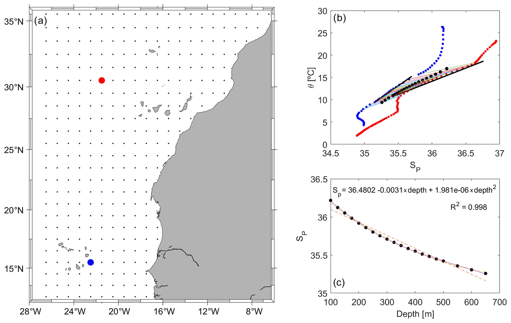
Figure 2(a) Map showing the two selected WOA stations in the ENACW (red) and SACW (blue) domains. (b) T–S diagram with the average salinity for each depth (in the range from 100 to 650 m) shown using black dots between the profiles of the northern and southern WOA stations. Observations at the same depths are connected by a straight line. (c) Linear, quadratic and cubic fits for depth versus salinity with the quadratic fit equation.
The SEALEVEL_GLO_PHY_L4_REP_OBSERVATIONS _008_047 product issued by the Copernicus Marine Environment Monitoring Service (CMEMS; http://marine.copernicus.eu, last access: 4 April 2019) provided the Level 4 Sea Surface Height (SSH) and derived variables as surface geostrophic currents, measured by multi-satellite altimetry observations over the global ocean with a spatial resolution of 0.25 ∘. These data captured the mesoscale structures and were helpful to validate the near-surface geostrophic field produced by the inversion.
GLORYS 12V1 (GLOBAL_REANALYSIS_PHY _001_030) outputs from 25 years, also issued by CMEMS, were used to estimate a summer climatology for the velocity field, temperature and salinity, with a horizontal resolution of ∘ at 50 standard depths. Specifically, the climatological salinity was used to present the CVF spatial distribution within the domain (see Sect. 3.2, Fig. 10a).
Data treatments (in situ, operational and modeling), interpolations with Data-Interpolating Variational Analysis (DIVA, Troupin et al., 2012), graphical representations, and the inverse model were coded in MATLAB (MATLAB, 2019). Finally, the Smith–Sandwell bathymetry V19.1 (Smith and Sandwell, 1997) was used in all maps and full-depth vertical sections.
2.3 Merged hydrographic dataset
A high-resolution in situ temperature field (T) was produced after merging the CTD and XBT profiles. The remaining variables were interpolated to this same new high-resolution grid to perform additional data treatments.
SP, O2, NO3, PO4 and SiO4H4 were optimally interpolated with DIVA at each transect independently. Before carrying out these interpolations, DIVA was applied to the T suppressing one XBT profile from each transect to validate the method. In fact, the interpolated values had a relative error <3.5 % in 75 % of cases. This allows one to set the signal-to-noise ratio (λ) and the horizontal and vertical correlation lengths (Lx and Ly). Hence, the interpolations of the remaining hydrological and biogeochemical variables were carried out with the following parameters: λ=4, Lx=110–135 km and Ly=50 m. Despite the fact that each variable behaves differently depending on its physical, chemical or biological nature, the correlation scales were considered the same due to the limitation of the sampling resolution. DIVA provided error maps for the gridded fields of each variable which allowed us to check their accuracy and spatial distribution. A total of 75 % of the interpolated values of SP and O2 had a relative error ≤ 3.5 %. Due to the lower sampling resolution of NO3, PO4 and SiO4H4, their interpolated values had higher errors. Between 70 % and 75 % of the interpolated values had a relative error ≤ 5.7 %.
Once the interpolations were performed, Absolute Salinity (SA; McDougall et al., 2012) and potential and conservative temperatures (θ and Θ, respectively; McDougall and Barker, 2011) were calculated (IOC et al., 2010). In addition, Neutral Density (γn; Jackett and McDougall, 1997) was used as the density variable.
2.4 Tracking the Cape Verde Front
One of the main goals of our study was to estimate the lateral fluxes on the tropical and subtropical sides of the Cape Verde Front. For this, we first had to uncover the location of the front – both with respect to depth and along its spatial distribution – within the domain. The classical definition places the CVF where isohaline 36 meets the 150 m isobath. Here, we have developed a method to extend this definition vertically as follows: two climatological profiles from WOA18 representative of the ENACW and SACW consistent with the definitions given by Tomczak (1981) were selected (Fig. 2a). Those selected climatological profiles provide an average relationship between SP, θ and depth, which reveals that the traditional definition of the front is based on a salinity value (36) that indeed corresponds to equal contributions (50 %) of the ENACW and SACW at 150 m depth. Following the same reasoning of equal contributions, we calculated the climatological salinity that would define the front location at standard depths from 100 to 650 m (Fig. 2b).
Finally, three linear, quadratic and cubic relationships between salinity and depth were used to infer the salinity that would define the front location at any given depth. The quadratic relationship was finally chosen due to its tight fit to observations (R2=0.998) keeping the polynomial order as low as possible (Fig. 2c). Thus, the front location could be uncovered at the depths occupied by the three layers of central waters (CW).
2.5 Water masses' distribution
An optimum multiparameter method (OMP; Karstensen and Tomczak, 1998) was used to quantify the contribution to the observations of the following water types: upper and lower North Atlantic Deep Water (UNADW and LNADW, respectively), Labrador Sea Water (LSW), Mediterranean Water (MW), AAIW, Subpolar Mode Water (SPMW), SACW at 12 ∘C and 18 ∘C (SACW12 and SACW18), ENACW at 12 and 15 ∘C (ENACW12 and ENACW15), and Madeira Mode Water (MMW). The hydrographic variables used for the analysis were θ, SP, SiO4H4, and NO (, where RN=1.4 is the stoichiometric ratio of organic matter remineralization; Anderson and Sarmiento, 1994; Broecker, 1974). The reference values of these variables in the source region of each water type were extracted from the literature (Pérez et al., 2001; Álvarez and Álvarez-Salgado, 2009; Lønborg and Álvarez-Salgado, 2014) and WOA13 (Locarnini et al., 2013; Zweng et al., 2013; Garcia et al., 2014a, b). A linear system of normalized and weighted equations for θ, SP, SiO4H4, NO and mass conservation was solved to obtain the water type proportions in the observations. Considering the measurement error, the relative conservative nature and the variability in each variable, the weights assigned to the balance of SiO4H4, NO, θ and SP were 1, 2, 10 and 10, respectively. A weight of 100 was imposed on the mass conservation equation assuming the mass was fully conserved. On the other hand, in order to solve this undetermined system of equations, the water types were grouped in a maximum of four according to oceanographic criteria. In this way, the unknowns were reduced from 11 to 5 with the following groups of water types: (1) MW–LSW–UNADW–LNADW, (2) SPMW–AAIW–MW–LSW, (3) SACW12–ENACW12–SPMW–AAIW, (4) SACW18–ENACW15–SACW12–ENACW12 and (5) MMW–SACW18–ENACW15. Surface waters (< 100 dbar) were excluded from the analysis due to their nonconservative behavior. This OMP with high determination coefficients (R2>0.97) and low standard errors of the residuals of θ, SP, SiO4H4 and NO realistically reproduced the thermohaline and chemical fields during FLUXES-I (Valiente et al., 2021).
2.6 Inverse model setup
The lateral geostrophic velocities were calculated at the boundaries of the volume closed by hydrographic stations. Geostrophic velocities were referenced to (∼ 1333 m, Fig. 3). As an initial guess, the velocities at the reference level were those estimated from the climatological summer mean provided by GLORYS.

Figure 3γn vertical section during the FLUXES-I cruise produced with the CTD–XBT merged dataset. White dashed isoneutrals limit the different water type layers. The direction chosen for the representation of the transects is the course of the vessel. Distance is calculated with respect to the first station (2). The section is divided as follows: transect N from east to west (from station 2 to 12), transect W from north to south (from station 12 to 19), transect S from west to east (from station 19 to 28) and transect E from south to north (from station 28 to 3). The northwestern, southwestern and southeastern corners are indicated by three vertical pink lines at stations 12, 19 and 28, respectively. The sampling points of dissolved oxygen and inorganic nutrients used in this work are represented by black dots.
An inverse box model (Wunsch, 1978) was then applied to estimate a set of unknowns based on the assumption of mass, salt and heat conservation within a closed volume. The unknowns in the system are an adjustment of the initial reference-level velocities, an adjustment of Ekman transports and the freshwater flux. The reference-level velocity field was then used to estimate the absolute water mass transport through each transect of the cruise (Martel and Wunsch, 1993; Paillet and Mercier, 1997; Ganachaud, 2003a; Machín et al., 2006; Pérez-Hernández et al., 2013; Hernández-Guerra et al., 2017; Fu et al., 2018; Burgoa et al., 2020).
The cruise was carried out over 25 d – a time lag large enough for the structures to evolve during the sampling. This time lag is not generally an issue that would introduce a relevant bias in the calculations; however, in this case, we have a closed volume composed of four hydrographical legs, so trying to connect the eastern section with the northern one might introduce a large bias in the observations and, consequently, in the geostrophic velocity field. Hence, to avoid any imbalances induced by the temporal evolution of the system, the volume is closed with land instead of with the eastern transect. To do so, WOA18 climatological nodes were used to extend the N and S transects eastward (green dots in Fig. 1), where the climatological summer mean of GLORYS was also included at the reference level. Therefore, the geostrophic velocities at the reference level were modified with the inversion in the N, W and S transects, whereas those velocities kept their initial climatological summer mean values from GLORYS in transect E.
The model was made up of eight layers bounded by the free surface and eight isoneutrals (26.46, 26.85, 27.162, 27.40, 27.62, 27.82, 27.922 and 27.962 kg m−3), reproduced essentially from those defined by Ganachaud (2003a) for the North Atlantic Ocean (Fig. 3). The inverse model considered mass conservation and salinity anomaly conservation per layer and also over the whole water column (Ganachaud, 2003b). Heat anomaly was introduced only in the deepest layer where it was also considered conservative. Salinity and heat were added as anomalies to improve the conditioning of the model and reduce the linear dependency between equations (Ganachaud, 2003b). Therefore, the inverse model was composed of 19 equations (9 for mass conservation, 9 for salt anomaly conservation and 1 for heat anomaly conservation). Those equations were solved using a Gauss–Markov estimator for 69 unknowns, comprised of 65 reference-level velocity adjustments, 3 unknowns for the Ekman transport adjustments (one per transect) and 1 unknown for the freshwater flux.
It was necessary to provide the uncertainties related to the noise of the equations (Rnn) and the unknowns (Rxx) a priori in order to solve this undetermined system. Rnn and Rxx values are compiled in Table 1. The noise of each equation depends on the layer thickness, the density field and the variability in the velocity field (Ganachaud, 1999, 2003b; Machín et al., 2006). Thus, an analysis of the velocity variability was performed in the mean depths of the eight layers. The velocity variance at each layer was estimated from summer months in the 25 years of GLORYS data. These variances were transformed into transport uncertainty values by multiplying by density and the vertical area of the section involved (Rnn in Table 1). The uncertainty assigned to the total mass conservation equation was the sum of the uncertainties from the eight mass conservation equations. The equations for salt and heat anomaly conservation depend on the uncertainty of the mass transport, on the variance of these properties and, specifically, on the layer considered (Ganachaud, 1999; Machín, 2003). Therefore, the uncertainties for salt and heat anomaly equations were estimated as follows (Ganachaud, 1999; Machín, 2003): , where Rnn(Cq) was the uncertainty in the anomaly equation of the property (salt or heat anomaly); var(Cq) was the variance of this property; a was a weighting factor (4 in the heat anomaly, 1000 in the salt anomaly and 106 in the total salt anomaly); q was a given equation corresponding to a given layer. These variability estimates were then included in the inverse model as the a priori uncertainty of the noise of equations in terms of variances of mass, salt anomaly and heat anomaly transports.
Table 1A priori noise of equations corresponding to the surface water (SW), central water (CW), intermediate water (IW) and deep water (DW) levels and uncertainties of all unknowns of the inverse model.
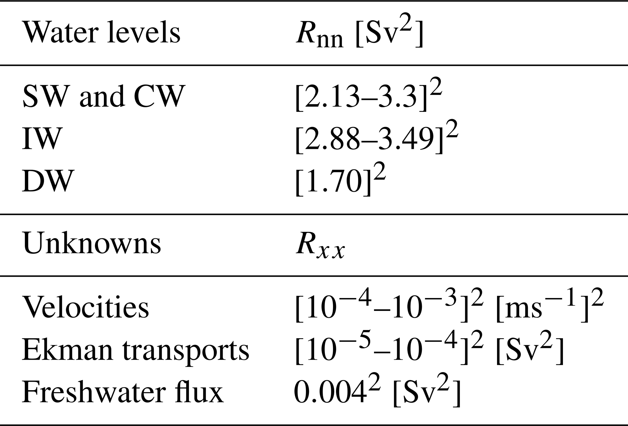
The variance of the velocities in the reference level was used as a measure of the a priori uncertainty for these unknowns. These variances were also calculated from the summer months' velocities provided by GLORYS (Rxx in Table 1).
The initial Ekman transports were estimated from the average wind stress during the days of the cruise. A 50 % uncertainty was assigned to the initial estimate of Ekman transports, related to the errors in their measurements and to the variability in the wind stress. An uncertainty of 50 % of the initial value of the freshwater flux, which was 0.0935 Sv, was also considered (Ganachaud, 1999; Hernández-Guerra et al., 2005; Machín et al., 2006). The Ekman transports, the freshwater flux and their uncertainties (Rxx in Table 1) were added to the inverse model in the shallowest layer for mass and salt anomaly as well as in the total mass transport and total salt anomaly transport equations.
Dianeutral transfers between layers were considered to be negligible compared with other sources of lateral transports, so they were not included in the inversion. Furthermore, the inverse model only works with information from the box boundaries and cannot be used to provide any spatial details of dianeutral fluxes for a given interface between layers, just an average value for the whole interface (Burgoa et al., 2020).
The resulting absolute geostrophic velocity field allowed us to calculate transports of O2 and inorganic nutrients. Those transports were obtained by multiplying their concentration by mass transports, so their concentrations were initially interpolated to the positions where the absolute geostrophic velocities were estimated.
3.1 Hydrography and water masses
The main water masses sampled during FLUXES-I were the ENACW (merging the MMW, ENACW15 and ENACW12) and the SACW (SACW18 and SACW12) below the mixing layer and above 700 m; the modified AAIW and MW from 700 up to 1700 m; and the North Atlantic Deep Water (the LSW and UNADW) below 1600 m (Figs. 3, 4, 5; Zenk et al., 1991; Martínez-Marrero et al., 2008; Pastor et al., 2012). Θ−SA definitions proposed by Tomczak (1981) for the salty and warm ENACW and the fresh and cold SACW (straight lines in Fig. 4) were used to identify CW in all transects: the main water mass sampled in transects N and W was the ENACW (∼ 36.15 g kg−1 at 300 m), whereas the SACW was dominant in transect S (∼ 35.65 g kg−1 at 300 m). Both the ENACW and SACW were registered along transect E. Water masses were also well defined at intermediate levels, with colder and fresher AAIW over warmer and saltier MW. MW was sampled mainly in transect N and in smaller proportions in the northern part of transects E and W, whereas the AAIW was the main water mass recorded in transects S, E and W (Fig. 4).
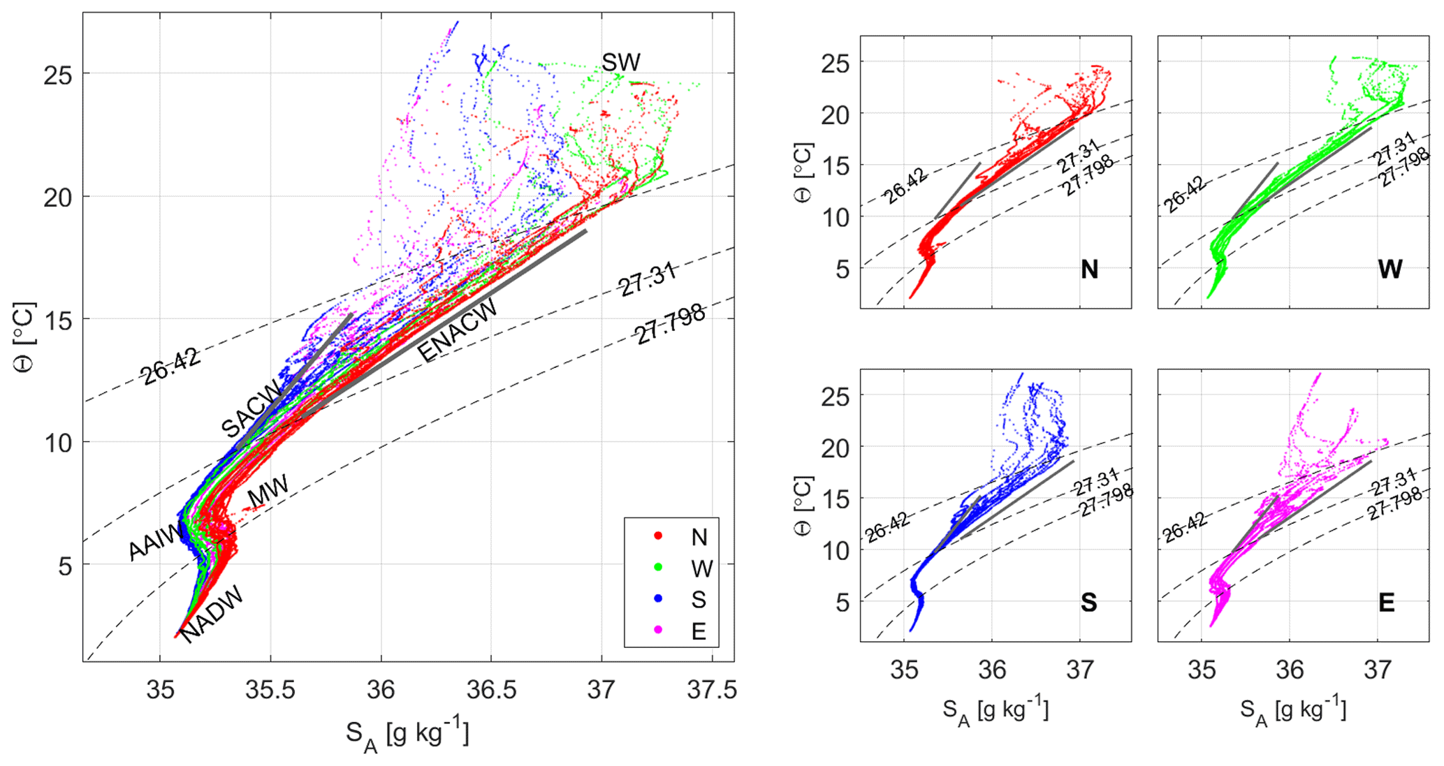
Figure 4Θ−SA diagrams during the FLUXES-I cruise. The different water masses in the northern (N, red dots), western (W, green dots), southern (S, blue dots) and eastern (E, pink dots) transects for surface waters (SW), North Atlantic Central Water (ENACW), South Atlantic Central Water (SACW), modified Antarctic Intermediate Water (AAIW), Mediterranean Water (MW) and North Atlantic Deep Water (NADW). Potential density anomaly contours (gray dashed lines) equivalent to 26.46, 27.4 and 27.922 kg m−3 isoneutrals delimit the surface, central, intermediate and deep water levels. Straight lines represent the Θ−SA relationship for ENACW and SACW equivalent to that proposed by Tomczak (1981).
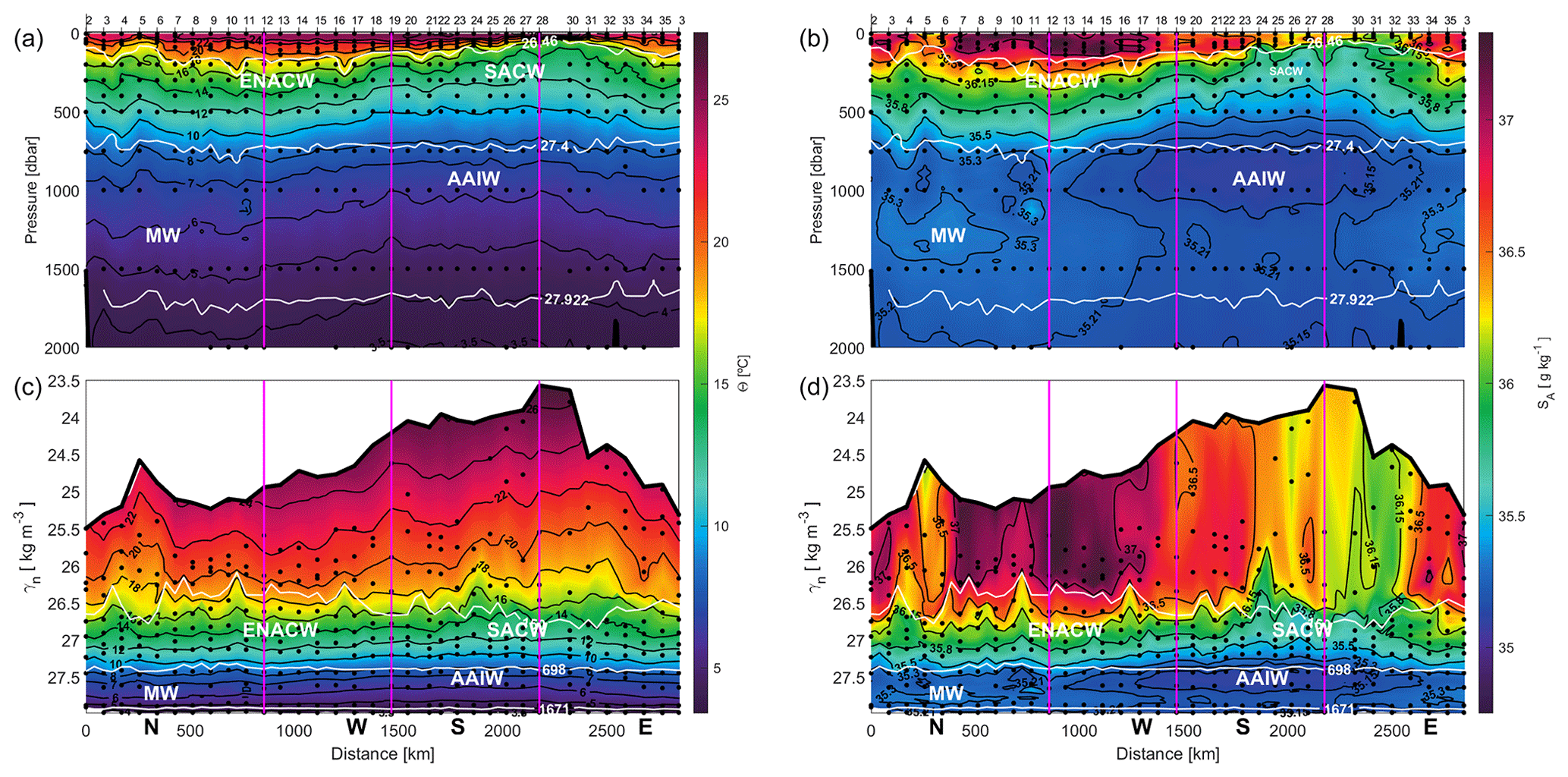
Figure 5Sections of Θ (a, c) and SA (b, d) with respect to depth (upper line) and γn (lower line) during the FLUXES-I cruise. The direction chosen for the representation is the same as in Fig. 3. The northwestern, southwestern and southeastern corners are indicated by three vertical pink lines at stations 12, 19 and 28, respectively. In depth sections, the isoneutrals that delimit the surface, central, intermediate and deep water are represented by white contours. In γn sections, the depths of 150, 698 and 1671 m are also shown. The sampling points for dissolved oxygen and inorganic nutrients used in this work are represented by black dots. Sections are only estimated with the CTD–XBT merged dataset.
Figure 3 presents the high-resolution γn field once the XBTs were considered. The upper four layers transported surface waters (SW, first layer above 26.46 kg m−3) and CW (between 26.46 and 27.40 kg m−3); intermediate waters (IW) flowed along the next three layers between 27.40 and 27.922 kg m−3, whereas deep waters (DW) flowed in the deepest layer below 27.922 kg m−3.
The overall distributions of O2, NO3, PO4 and SiO4H4 at CW were highly variable and closely related to the location of the different water masses. In transects N and W, where ENACW was dominant, the O2 concentrations were higher than in transects S and E where SACW was found, with minimum O2 values lower than 60 µmol kg−1 at 300 m (Fig. 6). In contrast, the concentrations of the three inorganic nutrients in these last two transects were higher than in transects N and W at CW levels, with concentrations of around 27–30 µmol kg−1 for NO3, 1.5–1.7 µmol kg−1 for PO4 and 7.5–9.9 µmol kg−1 for SiO4H4 at 300 m depth (Figs. 6, 7).
Figure 6Sections of O2 (a, c) and NO3 (b, d) with respect to depth (upper line) and γn (lower line) during the FLUXES-I cruise. The direction chosen for the representation is the same as in Fig. 3. The northwestern, southwestern and southeastern corners are indicated by three vertical pink lines at stations 12, 19 and 28, respectively. In depth sections, the isoneutrals that delimit the surface, central, intermediate and deep water are represented by white contours. In γn sections, the depths of 150, 698 and 1671 m are also shown. The sampling points of O2 and NO3 used in this work are represented by black dots.
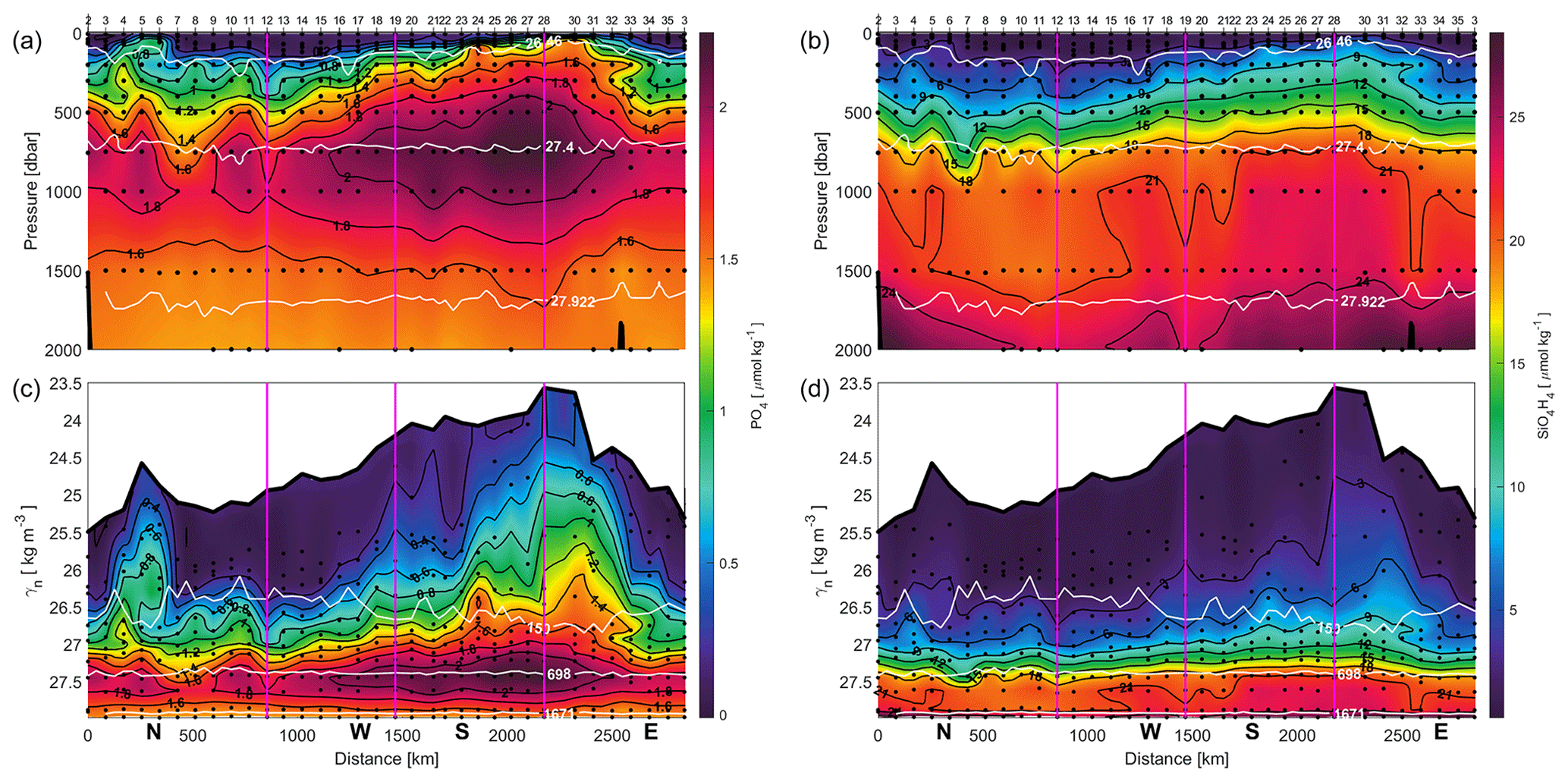
Figure 7Sections of PO4 (a, c) and SiO4H4 (b, d) with respect to depth (upper line) and γn (lower line) during the FLUXES-I cruise. The direction chosen for the representation is the same as in Fig. 3. The northwestern, southwestern and southeastern corners are indicated by three vertical pink lines at stations 12, 19 and 28, respectively. In depth sections, the isoneutrals which delimit the surface, central, intermediate and deep water are represented by white contours. In γn sections, the depths of 150, 698 and 1671 m are also shown. The sampling points of PO4 and SiO4H4 used in this work are represented by black dots.
In IW, the O2 distribution was quite uniform in all transects, presenting a slight increase with depth. With respect to inorganic nutrients, their concentrations in transect N were lower than in the remaining transects, which were occupied by a larger amount of AAIW. Indeed, the largest NO3 and PO4 concentrations were registered as being associated with AAIW at around 1000 m in transects S and E (Figs. 6, 7). Finally, in the deepest layer, high concentrations of O2 and inorganic nutrients were found. Specifically, the highest concentrations of SiO4H4 were recorded in this deepest layer.
The hydrological and biogeochemical characteristic of the water masses are summarized in Figs. 8 and 9, where the relationships between in situ measurements of SA, O2, NO3 and PO4 are displayed. These property–property distributions might be used to define the characteristic values of the water masses in the domain (Emery, 2001). In CW, inverse tight relationships are obtained for NO3 and PO4 with SA, whereas the relationship is direct and looser for O2 with SA. In IW, the relationships between NO3 and PO4 with SA are much less defined, with an “S”-like pattern. In all cases, the relationships between O2 and NO3 or O2 and PO4 are rather tight and inverse.
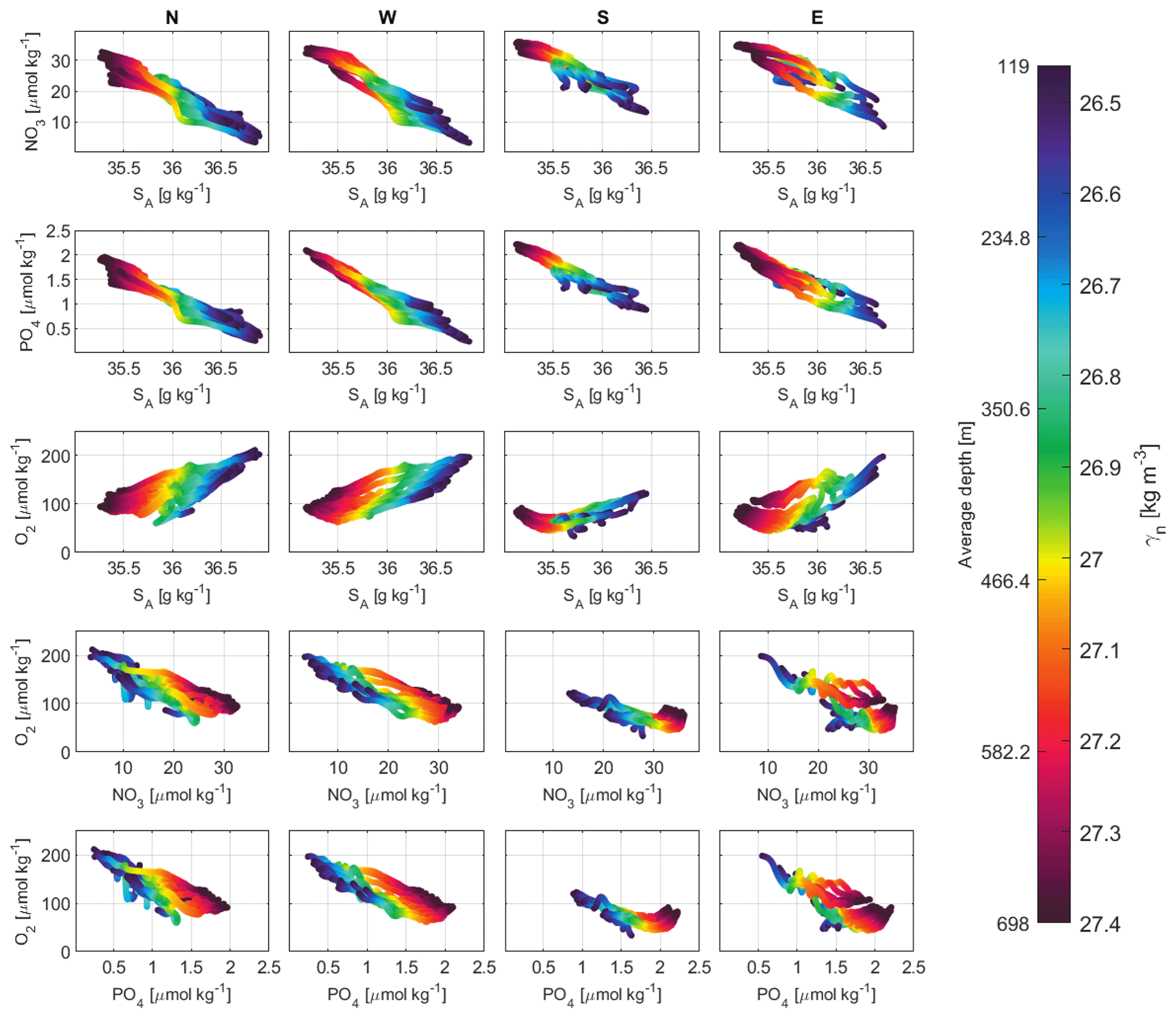
Figure 8Scatterplots of in situ observations of NO3 (first row), PO4 (second row) and O2 (third row) (in µmol kg−1) with respect to SA and γn (in color with an approximate scale of the average depths) in the north (N, first column), west (W, second column), south (S, third column) and east (E, fourth column) transects for CW layers. In the fourth and fifth rows, scatterplots of NO3–O2 and PO4–O2 in four transects for the CW layers are shown.
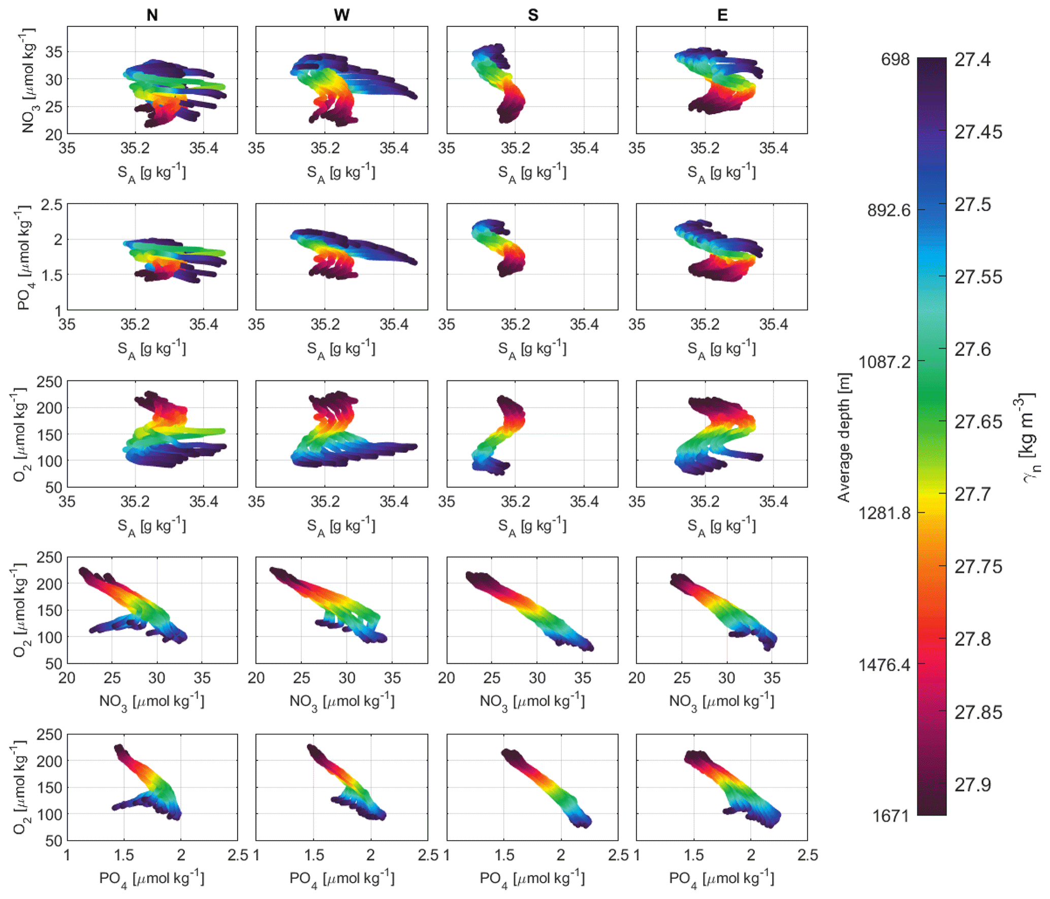
Figure 9Scatterplots of in situ observations of NO3 (first row), PO4 (second row) and O2 (third row) (in µmol kg−1) with respect to SA and γn (in color with an approximate scale of the average depths) in the north (N, first column), west (W, second column), south (S, third column) and east (E, fourth column) transects for IW layers. In the fourth and fifth rows, scatterplots of NO3–O2 and PO4–O2 in four transects for the IW layers are shown.
The previous distributions are presented from a large-scale perspective. A second reading of the dataset might be performed, emphasizing the role played by mesoscale structures. For instance, an intrathermocline anticyclonic eddy centered in station 4 was detected in Θ, SA, O2, NO3 and PO4 (Figs. 5, 6, 7). On the other side, the CVF was also detected in transects S and E as a sharp transition in all properties (Figs. 5, 6, 7). In particular, O2 presented two remarkable minimum values of 60 µmol kg−1 between 100 and 150 m when the frontal area was crossed (Fig. 6). Just below these O2 minima, the local maxima of NO3, PO4 and SiO4H4 were recorded (Figs. 6, 7).
3.2 Cape Verde Front
The CVF has historically been defined at only one depth, where isohaline 36 (or 36.15 g kg−1, Burgoa et al., 2020) intersects isobath 150 m (Zenk et al., 1991). Following that definition, the CVF could be located during FLUXES-I between stations 23 and 24 in transect S, where ΔSA>0.70 g kg−1 and ΔΘ>1.92 ∘C were observed between both sides of the front; CVF was also detected between stations 33 and 34 in transect E with lower ΔSA>0.30 g kg−1 and ΔΘ>1.10 ∘C values (Fig. 5).
The method developed in this paper to estimate the vertical location of the front depicted a complex spatial distribution (Fig. 10). The CVF is represented by several isohalines associated with specific depths. These isohalines unveil that the front was almost completely vertical in transect E, while in the southwestern corner it presented a notable slope with its surface end located south of its deep end. Hence, the front was oriented from northeast to southwest at near-surface layers, whereas it presented a roughly east–west orientation at 698 m depth (Fig. 10a). On the other hand, the CVF location presented with this methodology is indicated along the transects (pink lines), revealing a remarkable match with the distributions of the maximum contributions of ENACW (MMW–ENACW15–ENACW12) and SACW (SACW18–SACW12) estimated with the OMP (Fig. 10b, c).
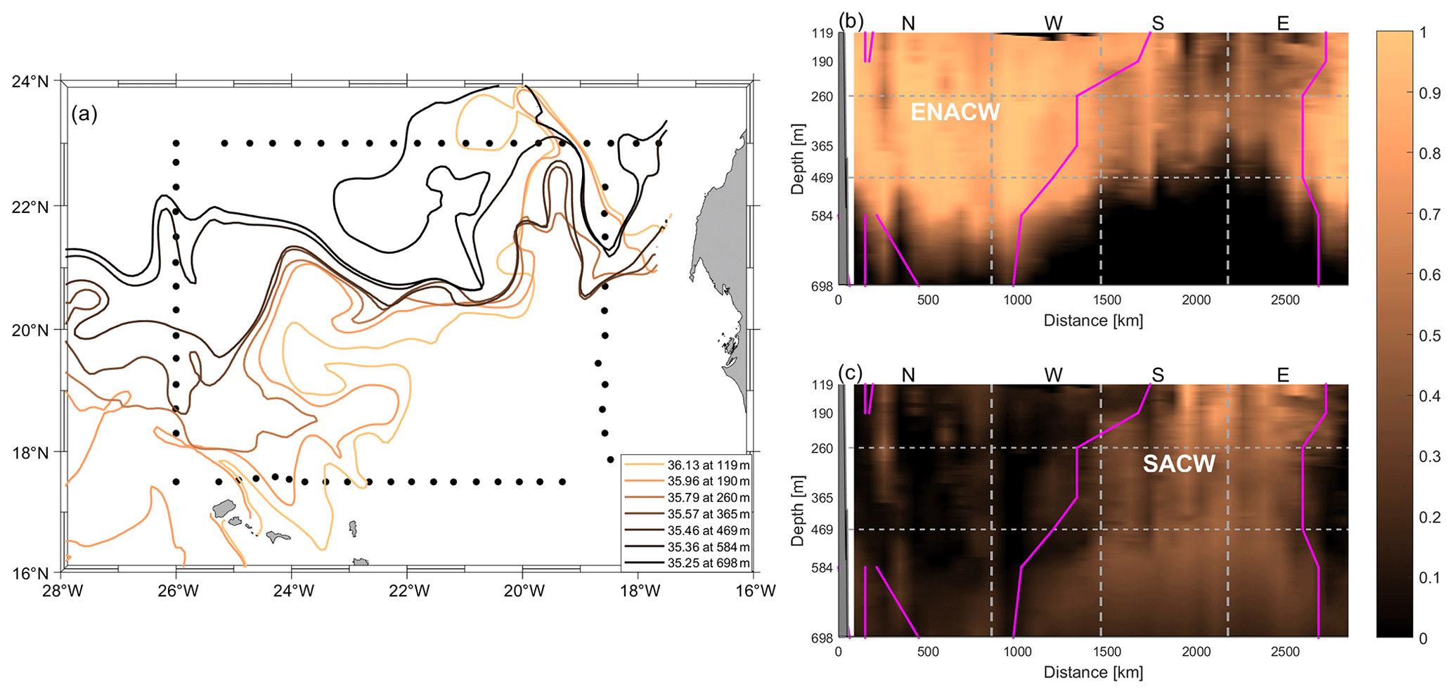
Figure 10(a) Location of the front at the 36.07, 35.88, 35.67, 35.43, 35.31, 35.2 and 35.08 isohalines, corresponding to average depths of 119, 190, 260, 365, 469, 584 and 698 m, equivalent to 26.46, 26.63, 26.85, 26.98, 27.162, 27.28 and 27.40 kg m−3, respectively. Vertical sections of the three layers of CW with the percentages of ENACW (b) and SACW (c), and the front location superimposed by pink lines. The direction chosen for the representation is the same as in Fig. 3. The northwestern, southwestern and southeastern corners are indicated by three vertical gray dashed lines. Three layers are also separated by two horizontal gray dashed lines.
3.3 Inverse model solution
The inverse model provided absolute geostrophic velocities for transects N, W and S, extended to the coast with WOA nodes. Mass transports were then evaluated to estimate the mass imbalance within the closed box. Figure 11 presents the mass transports accumulated along transects N, W and S, grouped by different water levels (panel a); the figure also shows the transports integrated per layer and transect (panel b). Note that positive (negative) values represent outward (inward) transports from (to) the closed box (). The mass transport imbalance in every water level was roughly zero once it was accumulated along the box, indicating that the mass was highly conserved (Fig. 11a). An imbalance was observed in the net transport mainly associated with the first and third layers (black line in Fig. 11b), likely related to mesoscale structures undersampled during the cruise.
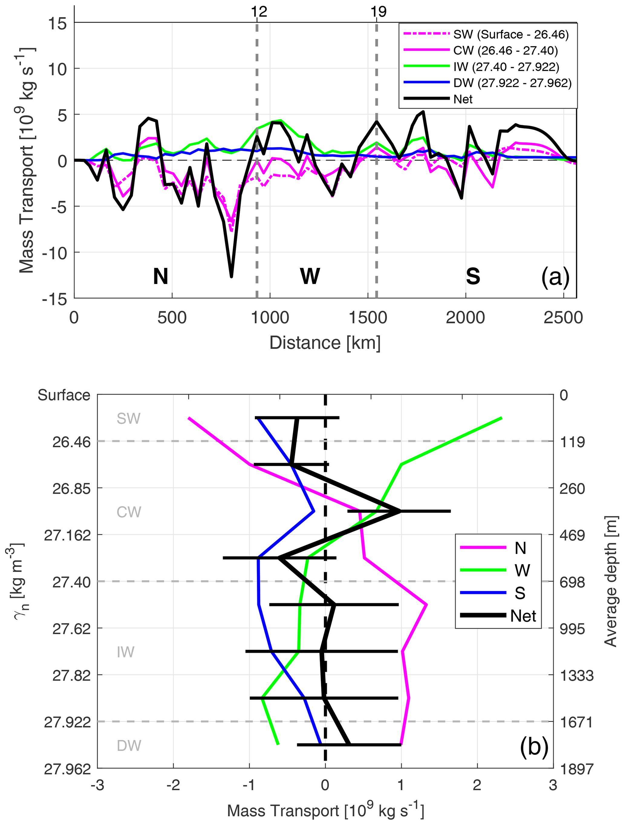
Figure 11(a) Accumulated mass transports per SW, CW, IW and DW levels, and (b) mass transports integrated per north, west and south transect, estimated by the inverse model during the FLUXES-I cruise (including WOA stations in transects N and S). Negative (positive) values indicate inward (outward) transports in both plots. Mass conservation in the whole domain close to the coast is shown by the black line. The northwestern and southwestern corners are indicated by vertical dashed lines at stations 12 and 19 in the accumulated mass transports (a). The horizontal bars in each layer represented by the net mass transport are the errors estimated by the inverse model (b).
Large transports are obtained in the entire water column. In the two shallowest layers, the mass exchange is basically from north and south to the west, carrying some 3.4 Sv. In the third and fourth layers, transports continued entering from the south, whereas transports reversed in the N and W transects, flowing a total of some 1 Sv. At IW levels, the estimated transports were moderately high and northward, with more than 3 Sv that entered through the W and S transects. At DW levels, the integrated mass transports were around 1 Sv, maintaining the IW levels' scheme.
The results obtained from the inversion are compared with two independent databases: transports from altimetry and transports from the GLORYS numerical model (Fig. 12). These transports are calculated by multiplying the velocity at the surface by the vertical area covered by the first layer in the inverse model. Accordingly, in the case of the inverse model we have used the accumulated mass transports in the first layer. The overall transport structure is rather similar for all three cases, in particular between the inverse model and the altimetry. GLORYS might not be recovering the mesoscale signal, and its low response to this variability is likely causing it to deviate from the other two databases. In all cases, the final imbalance is quite similar – about 1.5–2 Sv.
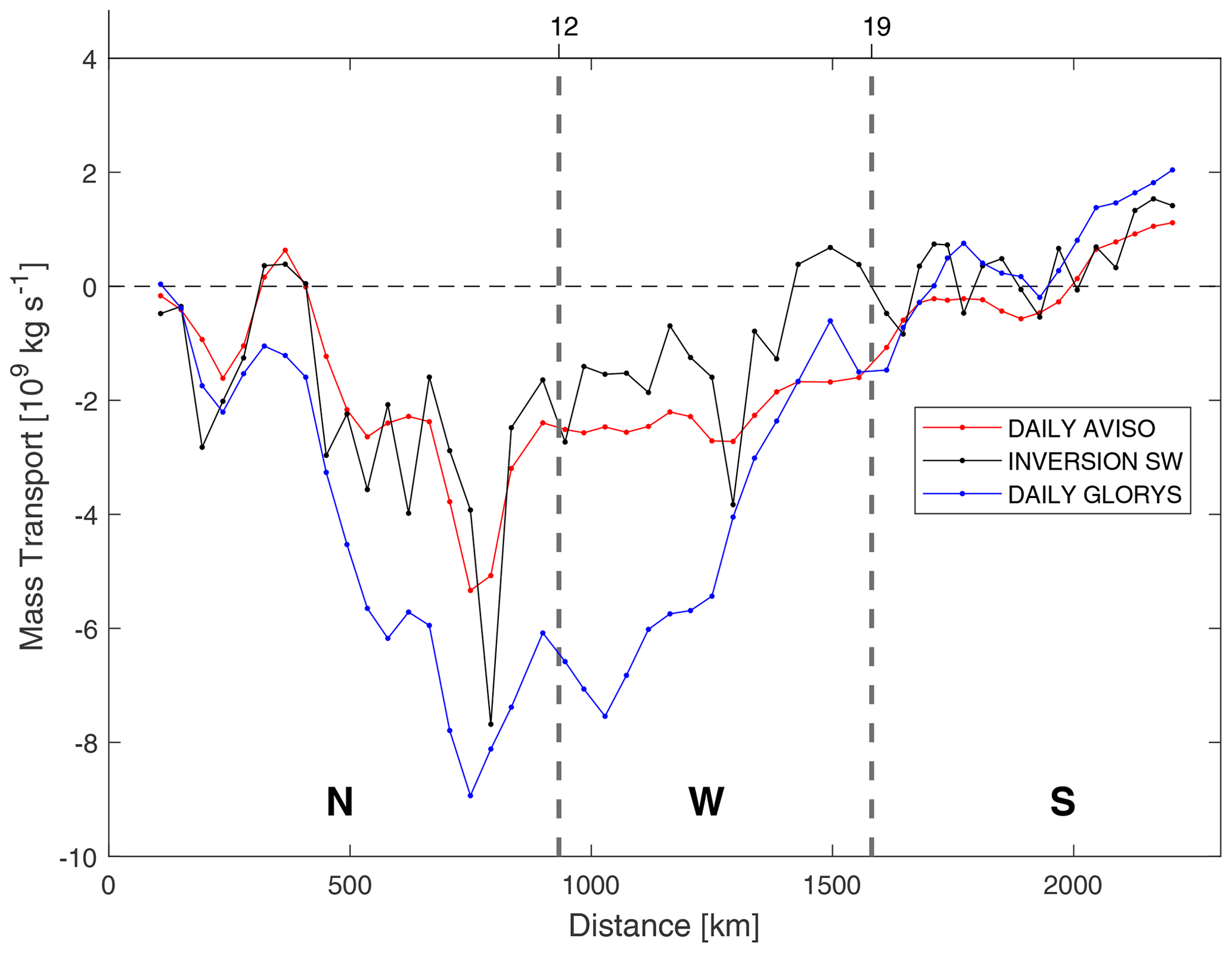
Figure 12Accumulated mass transports in the first layer of SW estimated along the N, W and S transects (without WOA stations) with altimetry-derived geostrophy (red line), inversion (with GLORYS data as reference velocities, black line) and the GLORYS field (blue line). Negative (positive) values indicate inward (outward) transports, as in Fig. 11. The northwestern and southwestern corners (at stations 12 and 19) are indicated by vertical dashed lines.
3.4 Geostrophic velocity
The previous result is now applied to present the geostrophic velocities along the three transects developed to perform the inverse model. Figure 13 displays the absolute velocity field perpendicular to each transect with a geographic criteria (positive velocities are northward and eastward). The absolute velocity field might be described as alternating vertical cells with velocities in the range from −0.25 to 0.25 m s−1; the largest velocities are mainly found in the upper 200–300 m depth.
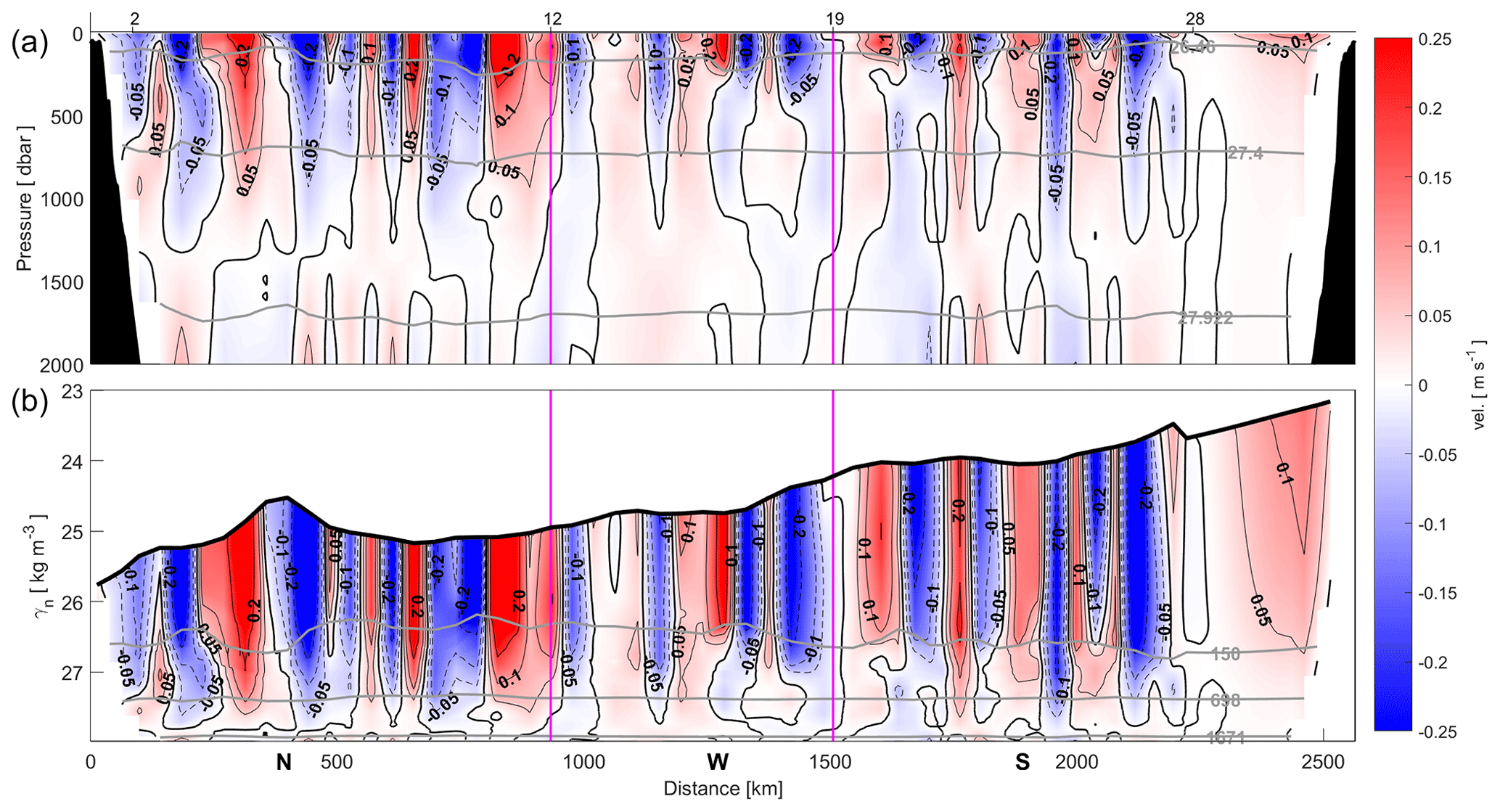
Figure 13Sections of the absolute geostrophic velocity perpendicular to each transect with respect to depth (a) and γn (b) during the FLUXES-I cruise (including WOA stations). The velocity sign was selected on geographic criteria (positive sign northward and eastward). The direction chosen for the representation is the same as in Fig. 3. The zero contour line is the thick black line. The northwestern and southwestern corners are indicated by vertical pink lines at stations 12 and 19. In depth sections, the isoneutrals that delimit the surface, central, intermediate and deep water are represented by gray contours. In γn sections, the depths of 150, 698 and 1671 m are also shown.
This velocity field helps to identify several mesoscale features captured during the cruise. Besides the intrathermocline anticyclonic eddy located between stations 3 and 5, another cyclonic eddy was centered between stations 5 and 7, next to the first eddy. Transect N was also crossed by a second anticyclonic eddy between stations 9 and 12. The main mesoscale structures sampled in transect W were a meander between stations 15 and 18 and an intrusion found between stations 18 and 19, which actually entered the box through the southwestern corner. A second part of this intrusion is observed in transect S, where it entered the box between stations 19 and 20 and left between stations 20 and 21. From stations 22 to 26, some additional meandering was observed along transect S. A cyclonic eddy had a notable negative velocity in the middle part of transect S centered at station 27.
3.5 Inorganic nutrient and O2 transports
The transports (integrated per water level and transect) for O2, NO3, PO4 and SiO4H4 are presented in Fig. 14 and compiled in Table 2. At IW and DW levels, the transports for all properties are nearly balanced and may be described as a net northward transport with contributions from the western and southern transects.
Table 2Mass transports and their errors (in Sv), and transports of O2, NO3, PO4 and SiO4H4 (in kmol s−1) with their errors relative to mass transport for SW, CW, IW and DW across the northern, western, southern and eastern transects for the FLUXES-I cruise (with WOA stations). Positive (negative) values indicate outward (inward) transports. The total row of each inorganic nutrient or O2 is its integrated transport throughout the whole water column. The last column is the maladjustment or imbalance of each water level.
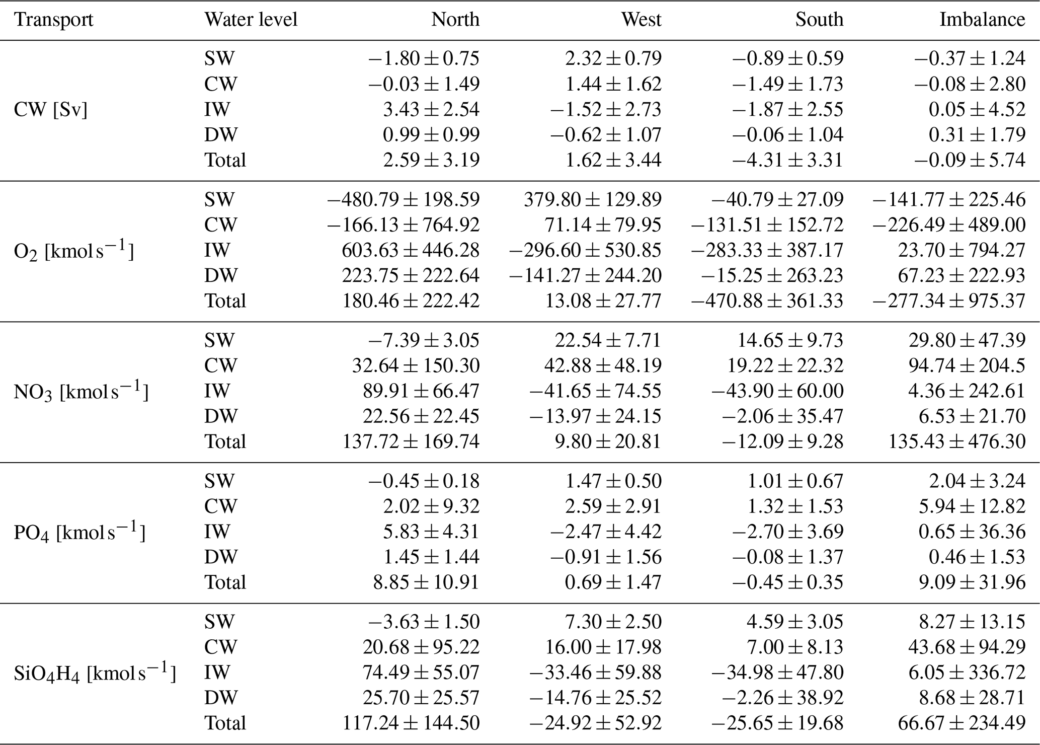
However, the transports at the SW and CW levels present an imbalanced distribution that can not be fully related to imbalances in the mass transports, as mass transports are nearly balanced at those water levels. Transports present a distribution where O2 enters the box through transects N and S; a lower amount of O2 leaves the box through transect W, revealing a net O2 decay within the box. The highest O2 transports are obtained at the SW levels, as a combined effect of large velocities and high O2 concentration in the photosynthetic layer in contact with the atmosphere. Finally, the pattern in the transports' distribution is quite the same for NO3, PO4 and SiO4H4: nutrients leave the domain through transects N, W and S, with a tiny amount entering the box through transect N at the SW and CW levels. The lowest transports for inorganic nutrients are obtained in the SW layer, as a consequence of nutrient depletion within the photic layer, whereas the highest transports are observed at CW and IW levels. A large imbalance is obtained at CW levels, providing a net nutrient increase within the box at CW levels.
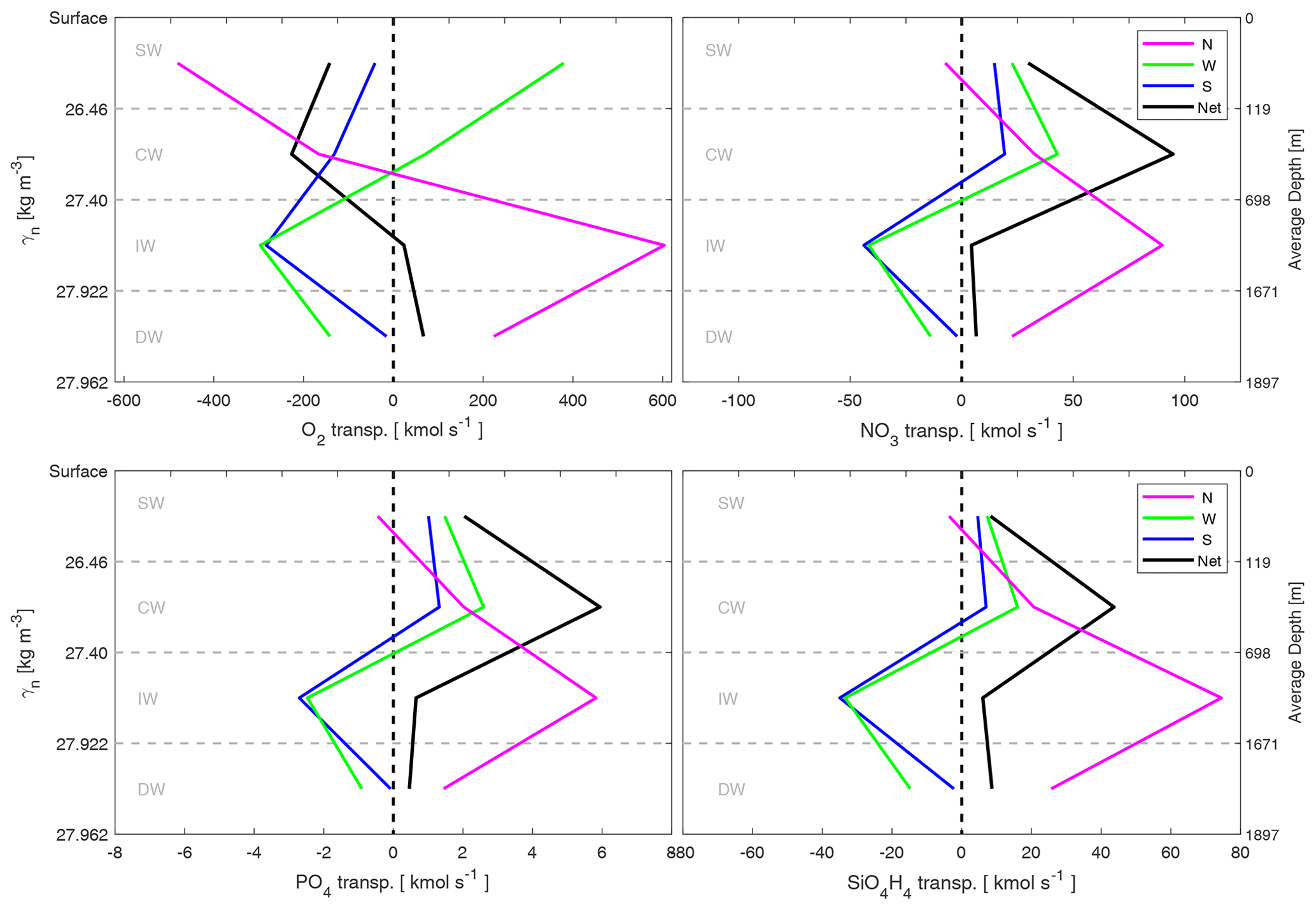
Figure 14O2, NO3, PO4 and SiO4H4 transports (in kmol s−1) integrated per water-type level (SW, CW, IW and DW) in the north (N, pink line), west (W, green line) and south (S, blue line) transects during the FLUXES-I cruise (including WOA stations). The black line represents the net transport of each biochemical variable. See Table 2 to check the O2, NO3, PO4 and SiO4H4 transports' values in each layer per transect. Negative (positive) values indicate inward (outward) transports, as in Fig. 11.
Biogeochemical budgets can be obtained for the entire water column once we have produced the net lateral transports of O2 and inorganic nutrients (Table 2). To do so, we first still need to estimate the O2 exchange between the sea surface and the atmosphere. We have proceeded as documented by Wanninkhof (2014), using an average wind speed for the whole domain (U, in m s−1) and the Schmidt number (Sc) for O2 to estimate the gas transfer velocity (k, in cm h−1) as . We then estimated the average apparent oxygen utilization (AOU); the O2 transport from the sea surface to the atmosphere is also estimated as , where A is the surface area of the domain (m2). These calculations provide an O2 export to the atmosphere of 113.54 kmol s−1. This number indicates that the total O2 consumption within the box is 163.8 kmol s−1, as the lateral transport integrated for the whole sampled water column was −277.34 kmol s−1. On the other hand, the inorganic nutrient positive balances indicate that the domain is producing inorganic nutrients, likely as a consequence of remineralization below the photic layer; the nutrient import from the atmosphere is considered negligible compared with lateral transports, according to climatological values reported by Fernández-Castro et al. (2019). Hence, this domain would be acting as an heterotrophic box, as revealed by the net oxygen consumption, with remineralization of N, P and Si below the photic layer.
We have presented the dynamics related to the water masses and their O2 and inorganic nutrient content in the transition between the eastern NASG and the NATG during summer 2017. The water masses' distribution in the CVFZ during FLUXES-I is consistent with that documented previously (Hernández-Guerra et al., 2005; Pastor et al., 2012; Peña-Izquierdo et al., 2012; Burgoa et al., 2020): a latitudinal change between the ENACW and SACW below the mixing layer and above 700 m was detected from north to south (Pelegrí et al., 2017), while a second latitudinal transition was observed in IW between AAIW and MW from south to north (Zenk et al., 1991), with AAIW being the dominant water mass. The characteristic of these water masses are conditioned by their origin and the path followed on their way to the CVB. While transects N and S present well-defined water masses, transects W and E reflect a water masses transition between transects N and S. The upwelling filaments off the coast of Cape Blanc are examples of mesoscale and submesoscale structures associated with the frontal systems. (Meunier et al., 2012; Lovecchio et al., 2018; Appen et al., 2020). The ENACW and SACW property distributions presented in Figure 8 compare well with those reported by Pastor et al. (2008) and Pelegrí and Benazzouz (2015b). At IW levels, the variability is mainly related to the AAIW flowing northward to the Canary Islands basin (Machín and Pelegrí, 2009; Machín et al., 2010). The shadow zone documented by Kawase and Sarmiento (1985) and the development of an oxygen minimum zone (OMZ) within the CW and IW levels was centered in transect S between 100 and 800 m depth with its core around 400 m between isoneutrals 27.1 and 27.3 kg m−3 (Karstensen et al., 2008; Brandt et al., 2015; Thomsen et al., 2019). That distribution matches well with the one provided by Peña-Izquierdo et al. (2015), with high concentrations of NO3 and PO4.
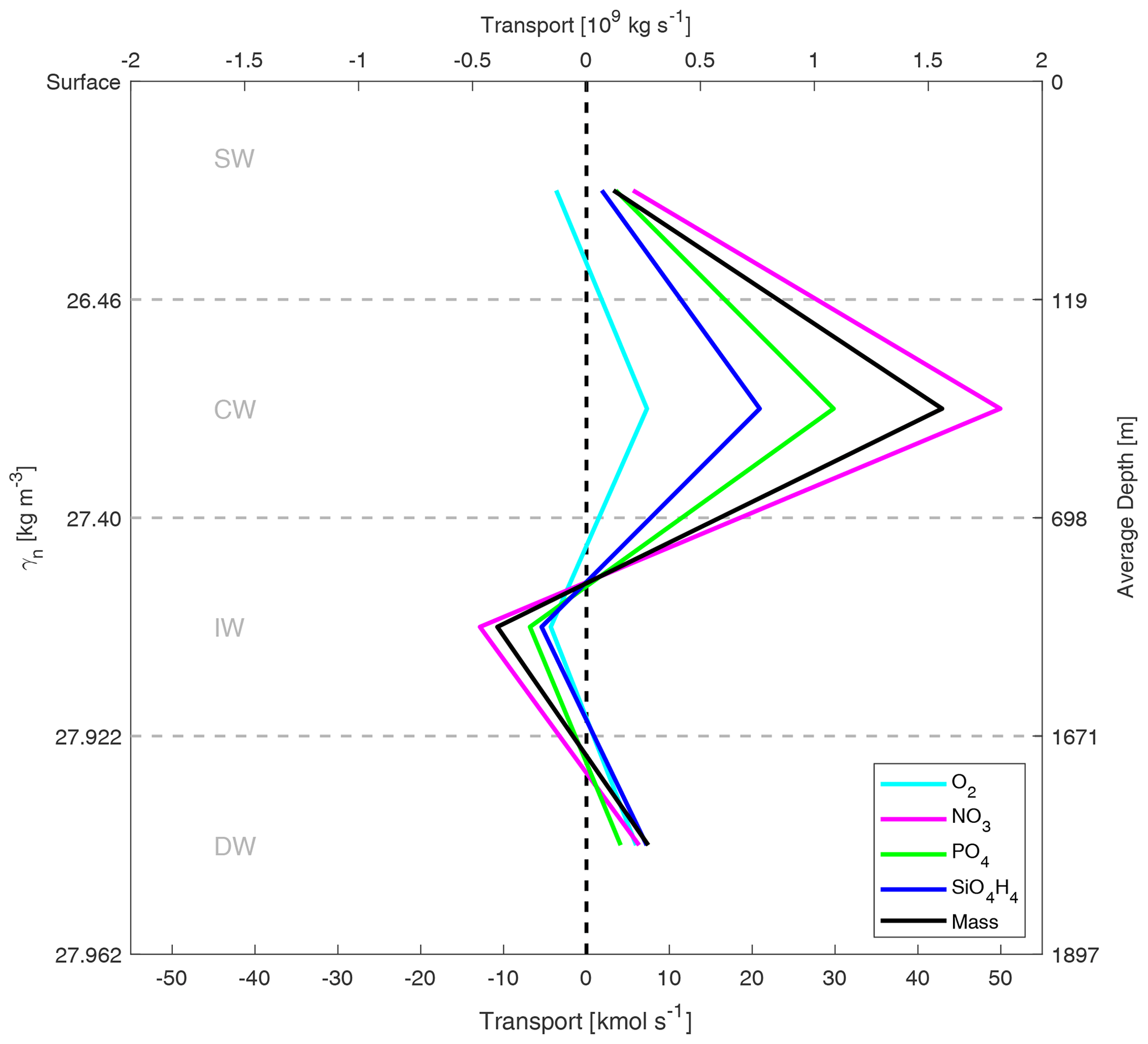
Figure 15Mass (109 kg s−1), O2, NO3, PO4 and SiO4H4 transports (in kmol s−1) integrated per water-type level (SW, CW, IW and DW) through transect E during the FLUXES-I cruise. Eastward transports were defined as positive. The O2 (PO4) transport is represented as being divided (multiplied) by 10.
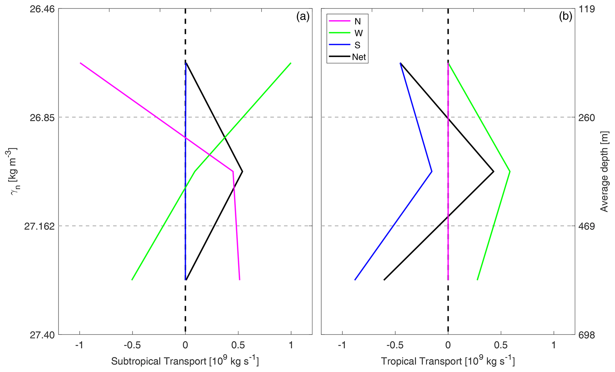
Figure 16Mass transports (109 kg s−1) integrated per transect north (N, pink line), west (W, green line) and south (S, blue line) of the subtropical (a) and tropical (b) areas separated by the CVF at the three CW layers (considering transports between WOA stations). The black line represents the net transport. Negative (positive) values indicate inward (outward) transports, as in Fig. 11.
A major contribution from this paper is the development of an extended version of the classical methodology applied to locate the CVF. Following the definitions of the SACW and ENACW reported by Tomczak (1981) and the interpretation of the CVFZ by Zenk et al. (1991), the front 3-D structure from 150 to 650 m depth has been produced by combining in situ and GLORYS data (Fig. 10). Fist of all, we would like to highlight the consistency between the results produced from the in situ observations compared to the results from the GLORYS model. The front spatial disposition reveals that the CVF is a complex meandering front with several associated mesoscale features, showing a variable geographical orientation at different depths (Barton, 1987; Martínez-Marrero et al., 2008; Pastor et al., 2008, 2012). The vertical distribution of the CVF enables the interpretation of the imbalances in lateral transports of mass, O2 and inorganic nutrients at both sides of the front (Table 3). The predominance (lack) of SACW (ENACW) in transect S suggests that the CVF may be functioning as a barrier against lateral transports across the front. The CVF also influenced its adjacent waters, as observed, for example, in the minima of O2 and the maxima of NO3 and PO4 sampled just below 150 m in the tropical side of the front, which might be indicating a local remineralization (Fig. 6) (Thomsen et al., 2019).
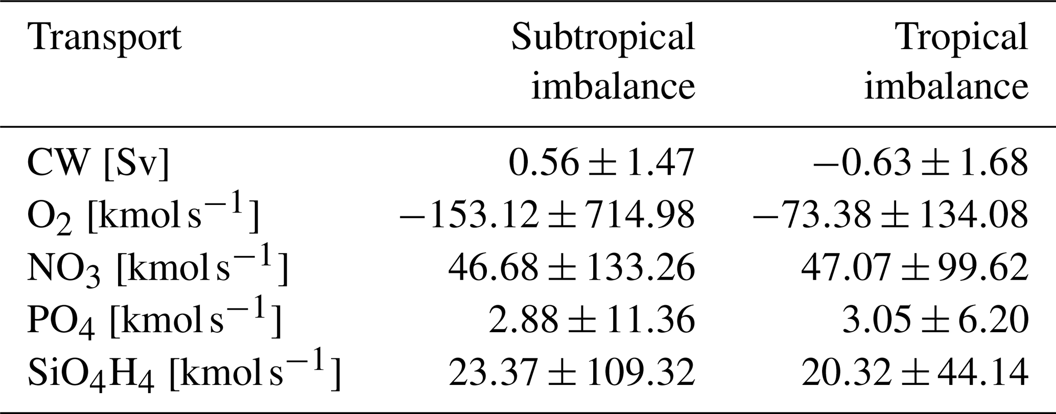
Table 3Total imbalances of mass, O2, NO3, PO4 and SiO4H4 transports in the subtropical and tropical areas separated by the CVF at the three CW layers. All imbalances are estimated from the integrated transports from each respective side of the front and considering transports between WOA stations.
The main limitations in the present analyzes were related to the high relative importance of mesoscale features in the domain. These features modify the thermohaline field with an intensity capable of inducing transports of approximately the same order of magnitude as those related to the large-scale circulation (Volkov et al., 2008; Zhang et al., 2014). On the one hand, if the mesoscale field is undersampled, it might induce large imbalances when quantifying the large-scale transports. On the other hand, the important dynamics associated with the mesoscale might also produce a lack of synopticity when the sampling takes longer than 15–20 d. These two effects might be responsible for the main limitations found in the dataset, as mesoscale structures were observed in almost all hydrographic sections. In turn, mesoscale structures impact on the physical–chemical variables in the domain, which might become significantly altered (Appen et al., 2020). A second limitation could be the absence of diapycnal transfers in the model. The imbalances diagnosed for the SW and CW would be reduced if a downwelling in the upper 300 m developed as a consequence of the upwelling relaxation during the cruise dates.
The velocity field has a direct impact on the exchange of O2 and inorganic nutrients at intermediate and deep water levels. The net balanced northward transport carries some 827 kmol s−1 of O2, 112 kmol s−1 of NO3, 7.3 kmol s−1 of PO4 and 100 kmol s−1 of SiO4H4. These values are well above the horizontal advection estimated from climatological data reported by Fernández-Castro et al. (2019) at intermediate and deep levels. However, the net horizontal transports presented in both analyses have very small values in intermediate and deep waters.
On the other hand, at surface and central levels the role played by biogeochemical processes also needs to be considered to outline the full picture of the processes forcing the variability in the O2 and inorganic nutrient transports. A westward imbalanced transport of O2 is observed at SW and CW levels, with a deficit of some 368 kmol s−1 related to the lower O2 concentration in the outflowing compared with the inflowing waters (Fernández-Castro et al., 2019). With respect to nutrients at these levels, the domain acts as a source, with net outward transports through the three transects of some 125 kmol s−1 for NO3, 8 kmol s−1 for PO4 and 52 kmol s−1 for SiO4H4. The western section presents the highest outward transports for the three nutrients at SW and CW levels, as in Fernández-Castro et al. (2019); our transports, however, are much larger than the climatological values provided by these authors. The calculations performed for the whole box, where the O2 export to the atmosphere was considered, somehow define a pattern for the offshore export of inorganic nutrients as a consequence of O2 consumption followed by nutrient remineralization below the photic layer. In this case, we would not expect the result to fit within the Redfield ratio as we are working with the whole box instead of differentiating between the surface layer (where oxygen production and nutrient consumption dominate) and the layers below (where net oxygen consumption and inorganic nutrient mineralization occurs). To do so, we would need to deal with the surface layer separately and estimate the role played by vertical advection and turbulence; this approach is beyond the scope of this study.
Despite the fact that the eastern section was not part of the inverse model, it still may provide insights into the transports within the domain in a location quite close to the coastal upwelling (Fig. 15). Mass transports indicate eastward transport at SW, CW and DW levels, whereas the transports reverse westward at IW levels. Transports related to O2 and inorganic nutrients reflect a similar pattern. O2 transports are close to zero at SW and CW levels, likely as a result of the high relative importance of the OMZ in this eastern section. Nutrients at the SW level present low onshore transports, whereas their transports increase at CW levels. At the IW and DW levels, a straight relationship is also observed for O2 and inorganic nutrients when compared with the mass transports' pattern. Hence, in this eastern section, it seems that the physical forcing is the dominating factor explaining the variability in the transports.
Finally, the development of a frontal zone provides the opportunity to perform the transport analysis at both sides of the front, in the tropical and subtropical domains within CW levels (Table 3 and Fig. 16). The mass transport imbalance is less than 1 Sv on both sides of the front. The pattern associated with transports is consistent with a southwestward transport on the subtropical side and a westward transport in the tropical domain, consistent with previous authors such as Pastor et al. (2008). Once the O2 and inorganic nutrient transports are estimated on both sides, their behavior is quite similar, with a net O2 decay and a net increase of inorganic nutrients. The main difference between both sides is related to the transports of O2, which is lower on the tropical side, about a half of the subtropical value, presumably related to the larger extension of the OMZ in this particular area.
In summary, the circulation in the transition zone between the coastal upwelling and the interior ocean, in the vicinity of the Cape Verde Front, is described as a westward flow at surface and central levels, on both the tropical and subtropical sides of the front, transporting about 3.76 Sv. Below, at intermediate levels, the circulation is markedly northward, carrying about 3 Sv. Mesoscale features constitute a main source of variability in the circulation at these water levels. On the other hand, the Cape Verde Front is featured from 100 to 700 m depth throughout the domain sampled; it presents a large meandering structure with an orientation that varies with depth. Finally, the O2 and inorganic nutrient transports at central levels are conditioned by biogeochemical processes with a decrease in O2 and an increase in inorganic nutrients. At intermediate levels, the variability in the O2 and inorganic nutrient transports are highly conditioned by physical factors. Once the O2 export to the atmosphere is accounted for, the domain is revealed as an heterotrophic system due to O2 consumption, with remineralization of inorganic nutrients.
The code related to DIVA interpolations can be download and extract from http://modb.oce.ulg.ac.be/mediawiki/index.php/Diva_matlab, last access: 15 December 2019. Details regarding the inverse model construction are available in Francisco Machín's PhD thesis (Machín, 2003).
To access the FLUXES project data, please contact the main researchers of the project: Ángel Rodríguez-Santana (angel.santana@ulpgc.es), Javier Aristegui (javier.aristegui@ulpgc.es) and Xosé Antón Álvarez-Salgado (xsalgado@iim.csic.es).
AR, XAA and JA were the main researchers of the FLUXES project. MDG sampled and analyzed the O2. XAA and BFC collected and analyzed the inorganic nutrients and developed the optimum multiparameter method. NB conceived the formal analysis of the physical variables and the associated processes. NB, with supervision from FM, carried out all of the transport calculations and developed the method to find the front beyond 150 m. All authors participated in the scientific interpretation and discussed the main results. NB prepared the paper with support from FM and contributions from all co-authors.
The authors declare that they have no conflict of interest.
This work was carried out in the framework of the FLUXES project (grant no. CTM2015-69392-C3-3-R), funded by the Spanish National Research Program and the European Regional Development Fund (MINECO/FEDER). Nadia Burgoa is currently working on her PhD and is supported by a fellowship funded by the Spanish Ministry of Economy and Competitiveness. The authors wish to thank the reviewers and the editor for providing constructive feedback that helped to improve this paper.
This research has been financially supported by the ongoing E-IMPACT project (grant no. PID2019-109084RB-C2).
This paper was edited by Piers Chapman and reviewed by Josep L. Pelegrí and two anonymous referees.
Álvarez, M. and Álvarez-Salgado, X. A.: Chemical tracer transport in the eastern boundary current system of the North Atlantic, Cienc. Mar., 35, 123–139, 2009. a, b
Anderson, L. A. and Sarmiento, J. L.: Redfield ratios of remineralization determined by nutrient data analysis, Global Biogeochem. Cy., 8, 65–80, 1994. a
von Appen, W.-J., Strass, V. H., Bracher, A., Xi, H., Hörstmann, C., Iversen, M. H., and Waite, A. M.: High-resolution physical–biogeochemical structure of a filament and an eddy of upwelled water off northwest Africa, Ocean Sci., 16, 253–270, https://doi.org/10.5194/os-16-253-2020, 2020. a, b
Barceló-Llull, B., Sangrà, P., Pallàs-Sanz, E., Barton, E. D., Estrada-Allis, S. N., Martínez-Marrero, A., Aguiar-González, B., Grisolía, D., Gordo, C., Rodríguez-Santana, Á., Marrero-Díaz, Á., and Arístegui, J.: Anatomy of a subtropical intrathermocline eddy, Deep-Sea Res. Pt. I, 124, 126–139, 2017. a
Barton, E.: Meanders, eddies and intrusions in the thermohaline front off Northwest Africa, Oceanol. Acta, 10, 267–283, 1987. a
Barton, E. D.: The poleward undercurrent on the eastern boundary of the subtropical North Atlantic, Poleward flows along eastern ocean boundaries, Springer, New York, NY, 82–95, 1989. a
Benazzouz, A., Mordane, S., Orbi, A., Chagdali, M., Hilmi, K., Atillah, A., Pelegrí, J. L., and Hervé, D.: An improved coastal upwelling index from sea surface temperature using satellite-based approach–The case of the Canary Current upwelling system, Cont. Shelf Res., 81, 38–54, 2014a. a, b
Benazzouz, A., Pelegrí, J. L., Demarcq, H., Machín, F., Mason, E., Orbi, A., Peña-Izquierdo, J., and Soumia, M.: On the temporal memory of coastal upwelling off NW Africa, J. Geophys. Res. C, 119, 6356–6380, https://doi.org/10.1002/2013JC009559, 2014b. a
Bentamy, A. and Fillon, D. C.: Gridded surface wind fields from Metop/ASCAT measurements, Int. J. Remote Sens., 33, 1729–1754, 2012. a
Brandt, P., Bange, H. W., Banyte, D., Dengler, M., Didwischus, S.-H., Fischer, T., Greatbatch, R. J., Hahn, J., Kanzow, T., Karstensen, J., Körtzinger, A., Krahmann, G., Schmidtko, S., Stramma, L., Tanhua, T., and Visbeck, M.: On the role of circulation and mixing in the ventilation of oxygen minimum zones with a focus on the eastern tropical North Atlantic, Biogeosciences, 12, 489–512, https://doi.org/10.5194/bg-12-489-2015, 2015. a
Broecker, W.: “NO”A conservative-mass tracer, Earth Planet Sc. Lett., 23, 100–107, 1974. a
Burgoa, N., Machín, F., Marrero-Díaz, A., Rodríguez-Santana, A., Martínez-Marrero, A., Arístegui, J., and Duarte, C. M.: Mass, nutrients and dissolved organic carbon (DOC) lateral transports off northwest Africa during fall 2002 and spring 2003, Ocean Sci., 16, 483–511, https://doi.org/10.5194/os-16-483-2020, 2020. a, b, c, d, e
Capet, X., McWilliams, J. C., Molemaker, M. J., and Shchepetkin, A.: Mesoscale to submesoscale transition in the California Current System. Part II: Frontal processes, J. Phys. Oceanogr., 38, 44–64, 2008. a
Castellanos, P., Pelegrí, J. L., Campos, E. J., Rosell-Fieschi, M., and Gasser, M.: Response of the surface tropical Atlantic Ocean to wind forcing, Prog. Oceanogr., 134, 271–292, 2015. a
Ekman, V. W.: Über Horizontalzirkulation bei winderzeugten Meeresströmungen, R. Friedländer & Sohn, Berlin, 1923. a
Emery, W. J.: Water types and water masses, Enc. Ocean Sci., 6, 3179–3187, 2001. a
Fernández-Castro, B., Mouriño-Carballido, B., and Álvarez-Salgado, X. A.: Non-redfieldian mesopelagic nutrient remineralization in the eastern North Atlantic subtropical gyre, Prog. Oceanogr., 171, 136–153, 2019. a, b, c, d
Fu, Y., Karstensen, J., and Brandt, P.: Atlantic Meridional Overturning Circulation at 14.5∘ N in 1989 and 2013 and 24.5∘ N in 1992 and 2015: volume, heat, and freshwater transports, Ocean Sci., 14, 589–616, https://doi.org/10.5194/os-14-589-2018, 2018. a
Gabric, A. J., Garcia, L., Van Camp, L., Nykjaer, L., Eifler, W., and Schrimpf, W.: Offshore export of shelf production in the Cape Blanc (Mauritania) giant filament as derived from coastal zone color scanner imagery, J. Geophys. Res.-Ocean., 98, 4697–4712, 1993. a
Ganachaud, A.: Large-scale mass transports, water mass formation, and diffusivities estimated from World Ocean Circulation Experiment (WOCE) hydrographic data, J. Geophys. Res., 108, 3213, https://doi.org/10.1029/2002JC001565, 2003a. a, b
Ganachaud, A.: Error budget of inverse box models: The North Atlantic, J. Atmos. Ocean. Technol., 20, 1641–1655, 2003b. a, b, c
Ganachaud, A. S.: Large Scale Oceanic Circulation and Fluxes of Freshwater, Heat, Nutrients and Oxygen, Ph.D. thesis, Massachusetts Institute of Technology and Woods Hole Oceanographic Institution, 106–124, https://doi.org/10.1575/1912/4130, 1999. a, b, c, d
Garcia, H. E., Locarnini, R. A., Boyer, T. P., Antonov, J. I., Baranova, O. K., Zweng, M. M., Reagan, J. R., and Johnson, D. R.: World Ocean Atlas 2013, Vol. 3, Dissolved Oxygen, Apparent Oxygen Utilization, and Oxygen Saturation, NOAA Atlas NESDIS 75, p. 27, 2014a. a
Garcia, H. E., Locarnini, R. A., Boyer, T. P., Antonov, J. I., Baranova, O. K., Zweng, M. M., Reagan, J. R., and Johnson, D. R.: World Ocean Atlas 2013, Volume 4: Dissolved Inorganic Nutrients (phosphate, nitrate, silicate), NOAA Atlas NESDIS 76, p. 25, 2014b. a
Grasshoff, K., Ehrhardt, M., and Kremling, K.: Determination of nutrients, Methods of Seawater Analysis, WILEY-VCH, Germany, 159–228, 1999. a
Hempel, G.: The Canary Current:Studies of an Upwelling System, A Symposium held in Las Palmas, 11–14 April 1978, Secretariat of the International Council for the Exploration of the Sea, Copenhagen, 180, ISSN 0074-4336, 1982. a
Hernández-Guerra, A., Fraile-Nuez, E., López-Laatzen, F., Martínez, A., Parrilla, G., and Vélez-Belchí, P.: Canary Current and North Equatorial Current from an inverse box model, J. Geophys. Res.-Ocean., 110, 1–16, https://doi.org/10.1029/2005JC003032, 2005. a, b
Hernández-Guerra, A., Espino-Falcón, E., Vélez-Belchí, P., Pérez-Hernández, M. D., Martínez-Marrero, A., and Cana, L.: Recirculation of the Canary Current in fall 2014, J. Mar. Syst., 174, 25–39, https://doi.org/10.1016/j.jmarsys.2017.04.002, 2017. a
Hosegood, P., Nightingale, P., Rees, A., Widdicombe, C., Woodward, E., Clark, D., and Torres, R.: Nutrient pumping by submesoscale circulations in the mauritanian upwelling system, Prog. Oceanogr., 159, 223–236, 2017. a, b
Hughes, P. and Barton, E. D.: Stratification and water mass structure in the upwelling area off northwest Africa in April/May 1969, Deep-Sea Res. Oceanogr. Abstracts, 21, 611–628, https://doi.org/10.1016/0011-7471(74)90046-1, 1974. a
IOC, SCOR, and IAPSO: The international thermodynamic equation of seawater – 2010: Calculation and use of thermodynamic properties. Intergovernmental Oceanographic Commission, Manuals and Guides No. 56, UNESCO (English), 196 pp., 2010. a
Jackett, D. R. and McDougall, T. J.: A Neutral Density Variable for the World's Oceans, J. Phys. Oceanogr., 27, 237–263, 1997. a
Karstensen, J. and Tomczak, M.: Age determination of mixed water masses using CFC and oxygen data, J. Geophys. Res.-Ocean., 103, 18599–18609, 1998. a
Karstensen, J., Stramma, L., and Visbeck, M.: Oxygen minimum zones in the eastern tropical Atlantic and Pacific oceans, Prog. Oceanogr., 77, 331–350, 2008. a
Kawase, M. and Sarmiento, J. L.: Nutrients in the Atlantic thermocline, J. Geophys. Res.-Ocean., 90, 8961–8979, 1985. a
Lázaro, C., Fernandes, M. J., Santos, A. M. P., and Oliveira, P.: Seasonal and interannual variability of surface circulation in the Cape Verde region from 8 years of merged T/P and ERS-2 altimeter data, Remote Sens. Environ., 98, 45–62, https://doi.org/10.1016/j.rse.2005.06.005, 2005. a
Locarnini, R. A., Mishonov, A. V., Antonov, J. I., Boyer, T. P., Garcia, H. E., Baranova, O. K., Zweng, M. M., Paver, C. R., Reagan, J. R., Johnson, D. R., Hamilton, M., and Seidov, D.: World Ocean Atlas 2013, Volume 1: Temperature, NOAA Atlas NESDIS 73, p. 44, 2013. a
Locarnini, R. A., Mishonov, A. V., Baranova, O. K., Boyer, T. P., Zweng, M. M., Garcia, H. E., Reagan, J. R., Seidov, D., Weathers, K., Paver, C. R., and Smolyar, I.: World Ocean Atlas 2018, Volume 1: Temperature, NOAA Atlas NESDIS, 81, 52 pp., 2018. a
Lønborg, C. and Álvarez-Salgado, X. A.: Tracing dissolved organic matter cycling in the eastern boundary of the temperate North Atlantic using absorption and fluorescence spectroscopy, Deep-Sea Res. Pt. I, 85, 35–46, 2014. a
Lovecchio, E., Gruber, N., and Münnich, M.: Mesoscale contribution to the long-range offshore transport of organic carbon from the Canary Upwelling System to the open North Atlantic, Biogeosciences, 15, 5061–5091, https://doi.org/10.5194/bg-15-5061-2018, 2018. a
Luyten, J., Pedlosky, J., and Stommel, H.: The ventilated thermocline, J. Phys. Oceanogr., 13, 292–309, 1983. a
Machín, F.: Variabilidad espacio temporal de la Corriente de Canarias, del afloramiento costero al noroeste de África y de los intercambios atmósfera-océano de calor y agua dulce, Ph.D. thesis, Universidad de Las Palmas de Gran Canaria, available at: http://hdl.handle.net/10553/2118 (last access: 7 June 2021), 2003. a, b, c
Machín, F. and Pelegrí, J. L.: Northward penetration of Antarctic intermediate water off Northwest Africa, J. Phys. Oceanogr., 39, 512–535, 2009. a, b, c
Machín, F., Hernández-Guerra, A., and Pelegrí, J. L.: Mass fluxes in the Canary Basin, Prog. Oceanogr., 70, 416–447, https://doi.org/10.1016/j.pocean.2006.03.019, 2006. a, b, c, d, e
Machín, F., Pelegrí, J. L., Fraile-Nuez, E., Vélez-Belchí, P., López-Laatzen, F., and Hernández-Guerra, A.: Seasonal Flow Reversals of Intermediate Waters in the Canary Current System East of the Canary Islands, J. Phys. Oceanogr., 40, 1902–1909, https://doi.org/10.1175/2010JPO4320.1, 2010. a, b, c
Martel, F. and Wunsch, C.: The North Atlantic Circulation in the Early 1980s-An Estimate from Inversion of a Finite-Difference Model, J. Phys. Oceanogr., 23, 898–924, 1993. a
Martínez-Marrero, A., Rodríguez-Santana, A., Hernández-Guerra, A., Fraile-Nuez, E., López-Laatzen, F., Vélez-Belchí, P., and Parrilla, G.: Distribution of water masses and diapycnal mixing in the Cape Verde Frontal Zone, Geophys. Res. Lett., 35, 0–4, https://doi.org/10.1029/2008GL033229, 2008. a, b, c, d
MATLAB: version R2019b, The MathWorks Inc., Natick, Massachusetts, available at: https://www.mathworks.com/products/matlab.html (last access: 30 March 2021), 2019. a
McDougall, T. J. and Barker, P. M.: Getting started with TEOS-10 and the Gibbs Seawater (GSW) oceanographic toolbox, SCOR/IAPSO WG, 127, 1–28, 2011. a
McDougall, T. J., Jackett, D. R., Millero, F. J., Pawlowicz, R., and Barker, P. M.: A global algorithm for estimating Absolute Salinity, Ocean Sci., 8, 1123–1134, https://doi.org/10.5194/os-8-1123-2012, 2012. a
Meunier, T., Barton, E. D., Barreiro, B., and Torres, R.: Upwelling filaments off Cap Blanc: Interaction of the NW African upwelling current and the Cape Verde frontal zone eddy field?, J. Geophys. Res.-Ocean., 117, https://doi.org/10.1029/2012JC007905, 2012. a, b
Paillet, J. and Mercier, H.: An inverse model of the eastern North Atlantic general circulation and thermocline ventilation, Deep-Sea Res. Pt. I, 44, 1293–1328, https://doi.org/10.1016/S0967-0637(97)00019-8, 1997. a
Pastor, M. V., Pelegrí, J. L., Hernández-Guerra, A., Font, J., Salat, J., and Emelianov, M.: Water and nutrient fluxes off Northwest Africa, Cont. Shelf Res., 28, 915–936, 2008. a, b, c, d, e, f
Pastor, M. V., Peña-Izquierdo, J., Pelegrí, J. L., and Marrero-Díaz, Á.: Meridional changes in water mass distributions off NW Africa during November 2007/2008, Cienc. Mar., 38, 223–244, 2012. a, b, c, d
Pastor, M. V., Palter, J. B., Pelegrí, J. L., and Dunne, J. P.: Physical drivers of interannual chlorophyll variability in the eastern subtropical North Atlantic, J. Geophys. Res.-Ocean., 118, 3871–3886, https://doi.org/10.1002/jgrc.20254, 2013. a, b
Pelegrí, J. L. and Benazzouz, A.: Oceanographic and biological features in the Canary Current Large Marine Ecosystem, Chap. 3.4, Coastal Upwelling off north-west Africa, IOC Technical Series, 115, 2015a. a
Pelegrí, J. L. and Benazzouz, A.: Oceanographic and biological features in the Canary Current Large Marine Ecosystem, Chapter 4.1, Inorganic nutrients and dissolved oxygen in the Canary Current large marine ecosystem, IOC Technical Series, 115, 133–142, 2015b. a, b, c, d
Pelegrí, J. L., Arístegui, J., Cana, L., González-Dávila, M., Hernández-Guerra, A., Hernández-León, S., Marrero-Díaz, A., Montero, M. F., Sangrà, P., and Santana-Casiano, M.: Coupling between the open ocean and the coastal upwelling region off northwest Africa: Water recirculation and offshore pumping of organic matter, J. Mar. Syst. 54, 3–37, https://doi.org/10.1016/j.jmarsys.2004.07.003, 2005. a
Pelegrí, J. L., Marrero-Díaz, A., and Ratsimandresy, A. W.: Nutrient irrigation of the North Atlantic, Prog. Oceanogr., 70, 366–406, https://doi.org/10.1016/j.pocean.2006.03.018, 2006. a, b
Pelegrí, J. L., Peña-Izquierdo, J., Machín, F., Meiners, C., and Presas-Navarro, C.: Deep-Sea Ecosystems Off Mauritania, Chapter 3, Oceanography of the Cape Verde Basin and Mauritanian Slope Waters, Springer, 119–153, https://doi.org/10.1007/978-94-024-1023-5_3, 2017. a, b, c
Peña-Izquierdo, J., Pelegrí, J. L., Pastor, M. V., Castellanos, P., Emelianov, M., Gasser, M., Salvador, J., and Vázquez-Domínguez, E.: The continental slope current system between Cape Verde and the Canary Islands, Sci. Mar., 76, 65–78, https://doi.org/10.3989/scimar.03607.18C, 2012. a, b
Peña-Izquierdo, J., van Sebille, E., Pelegrí, J. L., Sprintall, J., Mason, E., Llanillo, P. J., and Machín, F.: Water mass pathways to the North Atlantic oxygen minimum zone, J. Geophys. Res.-Ocean., 120, 3350–3372, 2015. a, b, c, d, e, f, g
Pérez, F. F., Mintrop, L., Llinás, O., Glez-Dávila, M., Castro, C. G., Alvarez, M., Körtzinger, A., Santana-Casiano, M., Rueda, M. J., and Ríos, A. F.: Mixing analysis of nutrients, oxygen and inorganic carbon in the Canary Islands region, J. Mar. Syst., 28, 183–201, https://doi.org/10.1016/S0924-7963(01)00003-3, 2001. a
Pérez-Hernández, M. D., Hernández-Guerra, A., Fraile-Nuez, E., Comas-Rodríguez, I., Benítez-Barrios, V. M., Domínguez-Yanes, J. F., Vélez-Belchí, P., and De Armas, D.: The source of the Canary current in fall 2009, J. Geophys. Res.-Ocean., 118, 2874–2891, https://doi.org/10.1002/jgrc.20227, 2013. a
Pérez-Rodríguez, P., Pelegrí, J. L., and Marrero-Díaz, A.: Dynamical characteristics of the Cape Verde frontal zone, Sci. Mar., 65, 241–250, https://doi.org/10.3989/scimar.2001.65s1241, 2001. a
Powers, J. G., Klemp, J. B., Skamarock, W. C., Davis, C. A., Dudhia, J., Gill, D. O., Coen, J. L., Gochis, D. J., Ahmadov, R., Peckham, S. E., Grell, G. A., Michalakes, J., Trahan, S., Beniamin, S. G., Alexander, C. R., Dimego, G. J., Wang, W., Schwartz, C. S., Romine, G. S., Liu, Z., Snyder C., Chen, F., Barlage, M. J., Yu, W., and Duda, M. G.: The weather research and forecasting model: Overview, system efforts, and future directions, Bull. Am. Meteorol. Soc., 98, 1717–1737, 2017. a
Sangrà, P., Pascual, A., Rodríguez-Santana, Á., Machín, F., Mason, E., McWilliams, J. C., Pelegrí, J. L., Dong, C., Rubio, A., Arístegui, J., Marrero-Díaz, Á., Hernández-Guerra, A., Martínez-Marrero, A., and Auladell, M.: The Canary Eddy Corridor: A major pathway for long-lived eddies in the subtropical North Atlantic, Deep-Sea Res. Pt. I, 56, 2100–2114, https://doi.org/10.1016/j.dsr.2009.08.008, 2009. a, b
Siedler, G., Zangenberg, N., Onken, R., and Morlière, A.: Seasonal changes in the tropical Atlantic circulation: Observation and simulation of the Guinea Dome, J. Geophys. Res.-Ocean., 97, 703–715, 1992. a, b, c
Smith, W. H. F. and Sandwell, D. T.: Global Sea Floor Topography from Satellite Altimetry and Ship Depth Soundings, Science, 277, 1956–1962, https://doi.org/10.1126/science.277.5334.1956, 1997. a
Stramma, L.: Geostrophic transport in the warm water sphere of the eastern subtropical North Atlantic, J. Mar. Res., 42, 537–558, https://doi.org/10.1357/002224084788506022, 1984. a
Stramma, L. and Siedler, G.: Seasonal changes in the North Atlantic subtropical gyre, J. Geophys. Res.-Ocean., 93, 8111–8118, 1988. a
Thomas, L. N.: Formation of intrathermocline eddies at ocean fronts by wind-driven destruction of potential vorticity, Dynam. Atmos. Ocean., 45, 252–273, 2008. a
Thomsen, S., Karstensen, J., Kiko, R., Krahmann, G., Dengler, M., and Engel, A.: Remote and local drivers of oxygen and nitrate variability in the shallow oxygen minimum zone off Mauritania in June 2014, Biogeosciences, 16, 979–998, https://doi.org/10.5194/bg-16-979-2019, 2019. a, b
Tomczak, M.: The CINECA experience, Mar. Policy, 3, 59–65, https://doi.org/10.1016/0308-597X(79)90040-X, 1979. a
Tomczak Jr., M.: An analysis of mixing in the frontal zone of South and North Atlantic Central Water off North-West Africa, Prog. Oceanogr., 10, 173–192, https://doi.org/10.1016/0079-6611(81)90011-2, 1981. a, b, c, d, e
Troupin, C., Barth, A., Sirjacobs, D., Ouberdous, M., Brankart, J.-M., Brasseur, P., Rixen, M., Alvera-Azcárate, A., Belounis, M., Capet, A., Lenartz, F., Toussaint, M.-E., and Beckers, J.-M.: Generation of analysis and consistent error fields using the Data Interpolating Variational Analysis (DIVA), Ocean Modell., 52, 90–101, 2012. a
UNESCO: The international system of units (SI) in oceanography, Technical Paper in Marine Science, 45, 1–124, 1985. a
Volkov, D. L., Lee, T., and Fu, L.-L.: Eddy-induced meridional heat transport in the ocean, Geophys. Res. Lett., 35, https://doi.org/10.1029/2008GL035490, 2008. a
Wanninkhof, R.: Relationship between wind speed and gas exchange over the ocean revisited, Limnol. Oceanogr.-Method., 12, 351–362, 2014. a
Wunsch, C.: North Atlantic general circulation west of 50∘W determined by inverse methods, Rev. Geophys., 16, 583–620, 1978. a
Zenk, W., Klein, B., and Schroder, M.: Cape Verde Frontal Zone, Deep-Sea Res. Pt. A, 38, S505–S530, https://doi.org/10.1016/S0198-0149(12)80022-7, 1991. a, b, c, d, e, f
Zhang, Z., Wang, W., and Qiu, B.: Oceanic mass transport by mesoscale eddies, Science, 345, 322–324, 2014. a
Zweng, M. M., Reagan, J. R., Antonov, J. I., Locarnini, R. A., Mishonov, A. V., Boyer, T. P., Garcia, H. E., Baranova, O. K., Johnson, D. R., Seidov, D., and Biddle, M. M.: World Ocean Atlas 2013, Volume 2: Salinity, NOAA Atlas NESDIS 74, p. 39, 2013. a
Zweng, M. M., Reagan, J. R., Seidov, D., Boyer, T. P., Locarnini, R. A., Garcia, H. E., Mishonov, A. V., Baranova, O. K., Weathers, K., Paver, C. R., and Smolyar, I.: World Ocean Atlas 2018, Vol. 2, Salinity, NOAA Atlas NESDIS, 82, 50 pp., 2018. a