the Creative Commons Attribution 4.0 License.
the Creative Commons Attribution 4.0 License.
 | 19 Feb 2021
Structure and drivers of ocean mixing north of Svalbard in summer and fall 2018
Zoe Koenig
Eivind H. Kolås
Ilker Fer
The Arctic Ocean is a major sink for heat and salt for the global ocean. Ocean mixing contributes to this sink by mixing the Atlantic- and Pacific-origin waters with surrounding waters. We investigate the drivers of ocean mixing north of Svalbard, in the Atlantic sector of the Arctic, based on observations collected during two research cruises in summer and fall 2018. Estimates of vertical turbulent heat flux from the Atlantic Water layer up to the mixed layer reach 30 W m−2 in the core of the boundary current, and average to 8 W m−2, accounting for ∼1 % of the total heat loss of the Atlantic layer in the region. In the mixed layer, there is a nonlinear relation between the layer-integrated dissipation and wind energy input; convection was active at a few stations and was responsible for enhanced turbulence compared to what was expected from the wind stress alone. Summer melting of sea ice reduces the temperature, salinity and depth of the mixed layer and increases salt and buoyancy fluxes at the base of the mixed layer. Deeper in the water column and near the seabed, tidal forcing is a major source of turbulence: diapycnal diffusivity in the bottom 250 m of the water column is enhanced during strong tidal currents, reaching on average 10−3 m2 s−1. The average profile of diffusivity decays with distance from the seabed with an e-folding scale of 22 m compared to 18 m in conditions with weaker tidal currents. A nonlinear relation is inferred between the depth-integrated dissipation in the bottom 250 m of the water column and the tidally driven bottom drag and is used to estimate the bottom dissipation along the continental slope of the Eurasian Basin. Computation of an inverse Froude number suggests that nonlinear internal waves forced by the diurnal tidal currents (K1 constituent) can develop north of Svalbard and in the Laptev and Kara seas, with the potential to mix the entire water column vertically. Understanding the drivers of turbulence and the nonlinear pathways for the energy to turbulence in the Arctic Ocean will help improve the description and representation of the rapidly changing Arctic climate system.
- Article
(6602 KB) - Full-text XML
- BibTeX
- EndNote


The Arctic Ocean is a sink for salt and heat. Relatively warm and salty Atlantic waters enter the Arctic Ocean via Fram Strait and the Barents Sea through-flow, and colder and fresher Arctic waters exit flowing east of Greenland through the East Greenland Current. Annual average water mass transformation in the Arctic is about in salinity and ∘C in temperature (Tsubouchi et al., 2018). With the rapid and large sea ice decline, the Arctic Ocean is particularly vulnerable to climate change. In the near future we will enter a new regime, in which the interior Arctic Ocean is entirely ice-free in summer and sea ice is thinner and more mobile in winter (Guarino et al., 2020), which will have vast implications for the Arctic Ocean circulation, the marine ecosystems it supports and the larger-scale climate (Timmermans and Marshall, 2020). The heat contained in the Atlantic- and Pacific-origin waters has the potential to melt the entire sea ice if it reaches the surface (Maykut and Untersteiner, 1971). The estimated mean Arctic Ocean surface heat flux necessary to keep the sea ice thickness at equilibrium is 2 W m−2 (Maykut and McPhee, 1995), yet observations indicate mean surface heat fluxes of 3.5 W m−2 (Krishfield and Perovich, 2005). To assess the evolution of the sea ice, the oceanic heat in the Arctic must be monitored and understood.
Atlantic Water is a major component of the Arctic Ocean heat budget, with particular influence in the Atlantic sector. An important player in the transformation of the Atlantic Water is vertical mixing. The central Arctic is relatively quiescent (Fer, 2009; Lincoln et al., 2016). Microstructure measurements indicate turbulent kinetic energy dissipation in the halocline of the deep basins to be around 10−10 to 10−9 W kg−1 (Fer, 2009; Lincoln et al., 2016; Rippeth et al., 2015). The dissipation rates are estimated to be several orders of magnitude larger on the ocean margins than over the abyssal plain (Padman and Dillon, 1991; Lenn et al., 2011; Rippeth et al., 2015; Fer et al., 2015).
North of Svalbard is a location with enhanced mixing. It is also a key region for the Arctic Ocean heat and salt budget, as it is the gateway for Fram Strait inflow of Atlantic Water. The circulation of Atlantic Water here is complex, with several recirculations in Fram Strait and three main inflow branches including the Yermak Branch (YB; Cokelet et al., 2008), the Yermak Pass Branch (YPB; Koenig et al., 2017; Crews et al., 2019; Menze et al., 2019) and the Svalbard Branch (SB; Cokelet et al., 2008), all originating from the West Spitsbergen Current (WSC) (Fig. 1a). As the Atlantic Water flows eastward, it deepens and gets colder and fresher due to mixing with the surrounding waters.
Cooling and freshening of the Atlantic Water north of Svalbard result from different processes. Along the slope north of Svalbard, eddies are shed from the Atlantic Water Boundary Current (Våge et al., 2016; Crews et al., 2018), transporting 0.16 Sv (1 Sv = 106 m3 s−1) of Atlantic Water and 1.0 TW (1 TW = 1012 W) away from the boundary current. Large vertical turbulent fluxes can occur in localized regions. Strong tidal currents over bathymetric slopes and rough topography generate internal waves which are a major source of energy for increased turbulence dissipation rates (Padman et al., 1992; Rippeth et al., 2017; Fer et al., 2020b). Rippeth et al. (2015) showed that the Yermak Plateau is a hot spot for tidal mixing. Fer et al. (2015) suggested that in this region, almost the entire volume-integrated dissipation can be attributed to the loss of baroclinic tidal energy converted locally from the surface tides. In the Nansen Basin north of Svalbard, turbulence in the upper layer influences the sea ice cover. Peterson et al. (2017) found an average winter ocean-to-ice heat flux of around 1.4 W m−2, with episodic local upwelling events and proximity to Atlantic Water pathways increasing the heat fluxes by 1 order of magnitude. Meyer et al. (2017) presented 6 months of turbulence data collected from January to June 2015 during the N-ICE2015 campaign. The combination of storms and shallow Atlantic Water leads to the highest heat flux rates observed: ice–ocean interface heat fluxes averaged 100 W m−2 during peak events.
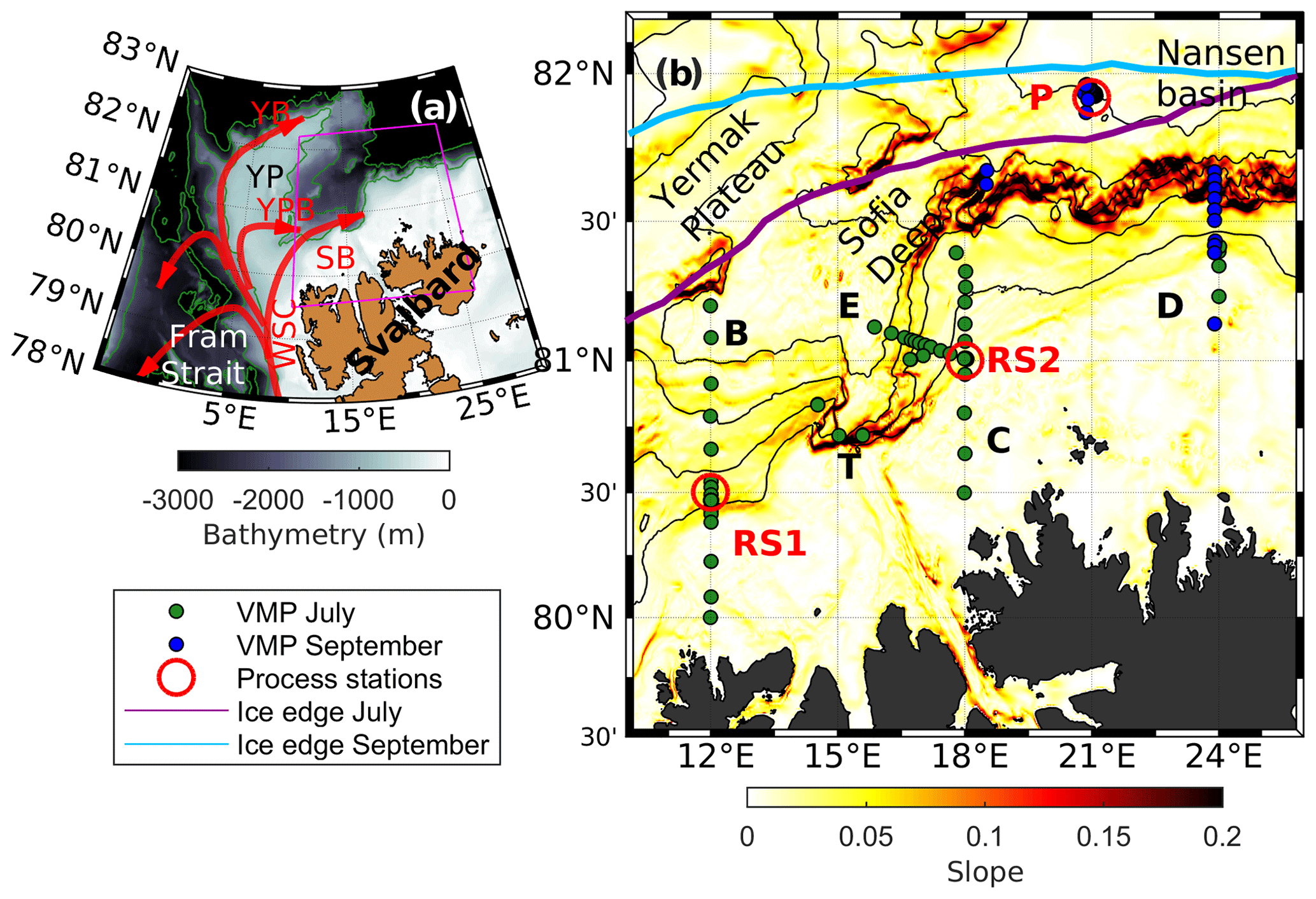
Figure 1(a) Circulation pattern of Atlantic Water around Svalbard, with the West Spitsbergen Current (WSC), the Svalbard Branch (SB), the Yermak Branch (YB) and the Yermak Pass Branch (YPB). Bathymetry is from the International Bathymetric Chart of the Arctic Ocean, IBCAO-v3 (Jakobsson et al., 2012). (b) Close-up of the magenta box in (a). Station locations (July, green dots; September, blue dots), sections (B, C, D and E) and process stations (red circles marked RS1, RS2 and P) are shown. The slope steepness calculated from IBCAO-v3 is color-coded in the background. Isobaths are drawn every 1000 m in (a) and 500 m in (b). Purple/light blue lines are the averaged sea ice edge defined as the 15 % ice concentration over the summer and fall cruise, respectively.
In the last decade, ice-free regions have been observed along the path of the Atlantic Water, in the Barents Sea first and then in the Eurasian Arctic Ocean, with warm and saline water extending up to the surface (Årthun et al., 2012; Ivanov et al., 2016). The lack of sea ice is mainly due to heat from the Atlantic layer reaching the surface (Duarte et al., 2020) and is associated with the Atlantification of the Eurasian Basin and of the Barents Sea (Polyakov et al., 2017; Årthun et al., 2012). In the Eurasian Basin, the upward oceanic heat flux towards the mixed layer has increased from 3–4 W m−2 in 2007–2008 to more than 10 W m−2 in 2016–2018 (Polyakov et al., 2020). This process is called the ice–ocean heat feedback as the increased ocean heat flux to the sea surface reduces ice thickness and increases its mobility, increasing atmospheric momentum flux into the ocean and reducing the damping of surface-intensified baroclinic tides (Polyakov et al., 2020). Mixing north of Svalbard is of particular interest to understand the Atlantification as it contributes to the cooling and freshening of the Atlantic Water entering the Arctic Ocean. The reduced ice cover over the continental slope north of Svalbard can be seen as a precursor of the entire Eurasian Basin and the processes therein. Indeed, Polyakov et al. (2020) documented an eastward lateral propagation of the so-called Atlantification, with a lag of about 2 years between the Barents Sea and the eastern Eurasian Basin. Therefore, detailed observations of the ocean dynamics north of Svalbard are needed to evaluate the active processes modifying the Atlantic Water layer in a changing Arctic, and their potential influence on the sea ice.
In this study we present observations of ocean turbulence north of Svalbard collected in summer and fall 2018 and focus on mechanisms which lead to turbulence in the different layers of the water column. Two main sources of ocean mixing are investigated: the wind and the tidal forcing. Turbulence production by background shear will not be addressed in this study as the vertical resolution (8 m) of the current data collected during the cruises is not sufficient to resolve shear instabilities.
Data were collected in 2018, during two cruises that took place north of Svalbard as a part of the Nansen Legacy Project. The summer cruise was on R/V Kristine Bonnevie from 27 June to 10 July 2018 (Fer et al., 2019), while the fall cruise was on the ice-class R/V Kronprins Haakon from 12 to 24 September 2018 (Fer et al., 2020a). During the cruises, several sections were repeated north of Svalbard across the continental slope, and three stations (two in July and one in September) were occupied for about 24 h to study mixing processes (Fig. 1b). Turbulence profiles were collected during both cruises (185 profiles in 9 d in July and 43 in 5 d in September) using a Vertical Microstructure Profiler (VMP). We calculated the Conservative Temperature (Θ) and Absolute Salinity (SA) using the International Thermodynamic Equations of SeaWater (TEOS-10) (McDougall and Barker, 2011).
2.1 Vertical Microstructure Profiler (VMP)
We used a 2000 m rated VMP manufactured by Rockland Scientific, Canada (RSI). The VMP is a loosely tethered profiler with a nominal fall speed of 0.6 m s−1. The profiler was equipped with pumped Sea-Bird Scientific (SBE) conductivity and temperature sensors, a pressure sensor, airfoil velocity shear probes, one high-resolution temperature sensor, one high-resolution micro-conductivity sensor and three orthogonal accelerometers. The microstructure data were processed using the routines provided by RSI (ODAS v4.01). Assuming isotropic turbulence, the dissipation rate of turbulent kinetic energy per unit mass, ϵ, can be expressed as
where ν is the kinematic viscosity equal to about m2 s−1 in these temperatures, the overbar denotes averaging in time and is the small-scale shear of one horizontal velocity component u. Dissipation rates were calculated from the shear variance obtained by integrating the shear vertical wavenumber spectra in a wavenumber range that is relatively unaffected by noise and corrected for the variance in the unresolved portions of the spectrum using an empirical model (Nasmyth, 1970). The shear spectra were computed using 1 s Fourier transform length and half-overlapping 4 s segments. We quality-screened the resulting values by inspecting the instrument accelerometer records, individual spectra and individual dissipation rate profiles from the two shear probes. We averaged estimates from both probes, except when their ratio exceeded 10, for example as a result of plankton hitting a sensor, and the lowest estimate was chosen. The noise level of the dissipation rate measured by the VMP is about (2–3) × 10−10 W kg−1. The temperature and salinity data from the VMP were compared against the ship's SBE CTD (conductivity, temperature, depth) profiles. A good agreement was observed and no correction was made. Dissipation measurements from the upper 15 m were excluded because of the disturbance from the ship's keel and the profiler's adjustment to free fall. The vertically integrated dissipation rate over a layer h (surface mixed layer or near-bottom layer in the following sections) is defined as (in W m−2) where ρ0=1027 kg m−3 is the seawater reference density.
We estimated the turbulent heat flux FH from
where Cp=3991.9 J kg−1 K−1 is the specific heat of seawater, Θ is the background temperature and κ is the diapycnal eddy diffusivity. We thus assume that turbulence diffuses the fine-scale temperature gradient at the same rate as the density gradient. The sign convention is that positive heat fluxes are directed upward in the water column.
We expressed the diapycnal diffusivity κ following Bouffard and Boegman (2013), where three states (energetic, transitional and buoyancy-controlled) are defined depending on the buoyancy Reynolds number, . In the transitional range (), calculation of κ is identical to Osborn (1980), using the canonical mixing coefficient of 0.2 (Gregg et al., 2018); however, in the energetic regime the latter is an overestimate. In our dataset, 80 % of the estimates are in the transitional regime. To compute κ, the buoyancy frequency or Brunt–Väisälä frequency, N, was approximated using , where g is the gravitational acceleration and σ0 is the potential density anomaly referenced to surface pressure. Background vertical gradients (for temperature, salinity and density) were taken over a 10 m length scale. To prevent spuriously large values of κ as N approaches neutral stratification, segments with buoyancy frequency below a noise level of s−2 were excluded.
We also computed the salt flux FS and the buoyancy flux FB:
where α and β are respectively the thermal expansion and salinity contraction coefficients, g is the gravitational constant, and the positive fluxes are directed upward.
In the rest of the study, sets of three to four consecutive repeat profiles at the process stations are averaged to avoid any bias toward these stations. Table 1 lists two numbers of “profiles”: the total number of casts performed (number of profiles) and the number of profiles used in analyses (n) after batch-averaging of consecutive repeat profiles. In the rest of the study, we always refer to the number of profiles after batch-averaging (in Figs. 4 and 7).
Table 1Overview of ocean microstructure measurements. The number of profiles used in analyses is n, after batch-averaging repeat profiles in the process stations.

2.2 Other datasets
We used the profiles collected from the ship's CTD system (Sea-Bird Scientific, SBE 911plus on both cruises) to check the temperature and salinity from the VMP. CTD data were processed using the standard SBE post-processing software, and salinity values were corrected against water sample analyses. Pressure, temperature and practical salinity data are accurate to ±0.5 dbar, ∘C, and , respectively.
The wind speed, direction and surface air temperature (Fig. 2) were recorded every minute during the cruises from the ship's weather station. The wind energy flux from the atmosphere into the ocean is estimated from the wind speed at 10 m height (U10) as (Oakey and Elliott, 1982), where ρair is the density of air and τ is the wind stress, parameterized using a quadratic drag with a drag coefficient Cd. We use the neutral drag coefficient at 10 m computed following Large and Pond (1981), adjusting the wind speed measured at 15 m height in July and 22 m height in September from the ship's mast to 10 m.
We used Arc5km2018 (Erofeeva and Egbert, 2020), a barotropic inverse tidal model on a 5 km grid, to estimate the tidal currents using the eight main constituents (M2, S2, N2, K2, K1, O1, P1 and Q1) and four nonlinear components (M4, MS4, MN2 and 2N2).
Bathymetric contours shown in maps are from the International Bathymetric Chart of the Arctic Ocean (IBCAO-v3) (Jakobsson et al., 2012). Station depths are from the ship's echosounder.
To discuss our findings in a broader scope, we used the global monthly isopycnal mixed-layer ocean climatology (MIMOC) at 0.5∘ resolution, which is objectively mapped with emphasis on data from the last decade (Schmidtko et al., 2013).
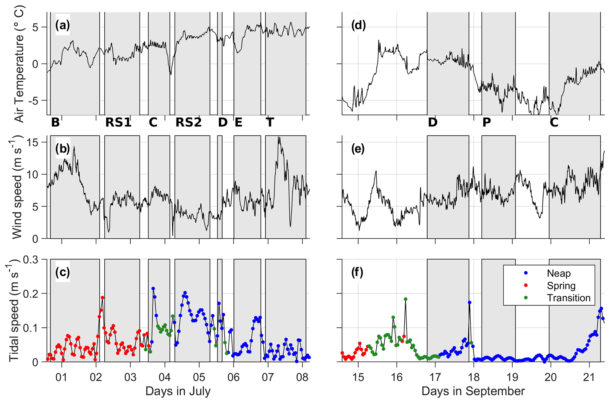
Figure 2Air temperature (a, d), wind speed (b, e) from the ship's weather station and tidal current speed (c, f) from the Arc5km2018 model. Panels (a)–(c) are during the July (Summer) cruise. Panels (d)–(f) are during the September (fall) cruise. Grey shading corresponds to the periods of turbulence measurements (sections or process stations). In (c) and (f), the tidal conditions during the time of sampling are indicated as neap, spring tide, and the transition between the neap and spring tide with blue, red and green dots respectively.
3.1 Environmental context
The cruises cover the summer and fall conditions, typically in open waters. Four main sections were occupied north of Svalbard: Section B, C and E in July, and section D in September, capturing the core of the inflowing Atlantic Water. Selected stations were occupied for 24 h to investigate mixing processes in detail at a specific location: T, RS1, RS2 and P (Fig. 1b). In September, turbulence profiling terminated after the winch broke, resulting in fewer profiles (section D, process study P and the outer deep stations at section C).
In July, the Yermak Plateau was covered by sea ice, and the ice edge was close to the continental slope north of Svalbard (Fig. 1), limiting the station coverage (e.g., section D could not be completed). We note that the sea ice encountered in July was closer to the continental slope at 24 ∘E than what is suggested by the sea ice edge from satellite, defined here as 15 % sea ice concentration. In September, the sea ice edge was ∼30 to 50 km further north, and the continental slope was entirely free of ice, which can facilitate enhanced wind energy input to the oceanic near-inertial currents (Rainville and Woodgate, 2009).
Air temperature differs between the two cruises: while it was mainly positive in July, the temperature dropped to −10 ∘C in September (Fig. 2a and d) near the sea ice edge. Over the two cruises, wind was moderate, peaking only for half a day to 15 m s−1 on 7 July (Fig. 2b). In September, the average wind speed was 8 m s−1 with no specific events. During the cruise in September, surface gravity waves were estimated using single-point ocean surface elevation data obtained from the bow of the ship using a system that combines an altimeter and inertial motion unit (Løken et al., 2019). The significant wave height varied between 0.5 and 1.5 m with mean wave periods between 2 and 6 s.
Tidal currents varied significantly during the cruise depending on the location, with a maximum amplitude about 20 cm s−1 during RS2 from 4 to 6 July. The tidal currents were stronger on the slope than in the deep basin (such as during P in the Nansen Basin). In July, sections were occupied during spring tides for the first 3 d and during neap tides for the rest of the cruise. In September, the tidal currents at the stations were weaker and mainly during neap tides, except for a short period of spring tides in the beginning of the cruise (around 15 September 2018).
3.2 Hydrography
Figure 3 shows the distribution of temperature and dissipation rate collected in sections and the process stations performed during the two cruises. Temperature sections were obtained by gridding the data in 1 km horizontal and 2 m vertical grid size using linear interpolation.
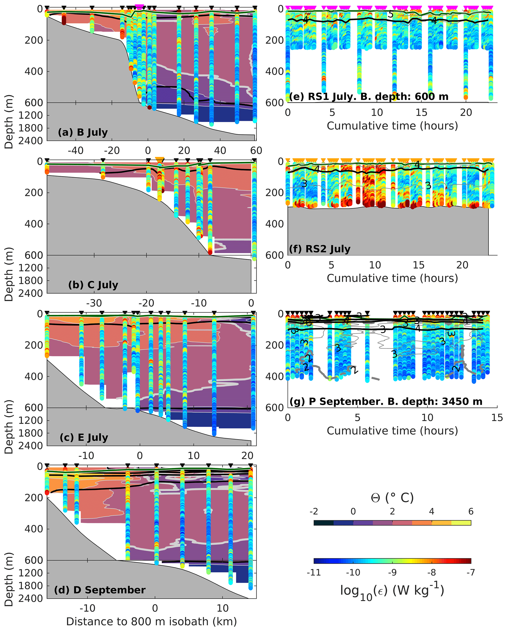
Figure 3Overview of the main sections (a–d) and the process study stations (e–g) during the July and September cruises. In (a)–(d), background is Θ, and the dissipation rate profiles (ϵ) are superimposed. Note the change of vertical scale at 600 m depth. In (e)–(g), temperature contours are shown as thin grey lines. In all panels, bold black lines are the isopycnals, and the thicker grey line is the 2 ∘C isotherm. Bathymetry is from the bottom depth measured at each station. Triangle markers are the time or location of the stations. In (a) and (b), the pink and orange station markers indicate the location of the RS1 and RS2 process station, respectively, shown in (e) and (f). At station P (g), one early VMP cast performed about 6 h before the start of the first shown profile is excluded. The horizontal axis is the distance to the 800 m isobath in the (a)–(d) and cumulative time from the first profile in (e)–(g). The dark green line is the mixed layer depth.
We estimate the mixed layer depth (dark green line in Fig. 3) as the depth at which the density exceeds the shallowest measurement by 0.01 kg m−3 in July and by 0.03 kg m−3 in September, because of the presence of meltwater at the surface in September. The vertical gradients are large, and the mixed layer depth is not very sensitive to the exact criterion. An estimate of a surface layer depth (not shown) following Randelhoff et al. (2017) was very similar.
The slope north of Svalbard is characterized by Atlantic Water flowing along the 800 m isobath. The Atlantic Water is defined as water masses with Θ>2 ∘C and kg m−3 following Rudels et al. (2000). The warm waters observed roughly between 500 and 1100 m isobaths are associated with the Atlantic Water core (section panels in Fig. 3 and blue line in Fig. 4a). Colder and fresher waters found offshore are Atlantic Water from Fram Strait, which has been modified by mixing with the surrounding waters. A thorough description of the hydrography and circulation during the two cruises can be found in Kolås et al. (2020).
We calculated average profiles of temperature, salinity, dissipation rate and diffusivity using data combined from both July and September cruises. The averaging is made in isopycnal coordinates to account for the possible vertical displacement of isopycnals and water masses from the slope to the deep basin. Once averaged, the profiles are mapped onto vertical coordinates using the corresponding average depth of an isopycnal (Fig. 4). While this averaging is representative of the vertical structure below the mixed layer, it is probably not appropriate for the surface layer where surface stratification and buoyancy flux are significantly different in July and September (see the following section for more details). The average profiles are obtained in subsets, depending on their distance from the 800 m isobath, which is representative of the mean location of the core of the inflowing Atlantic Water (Kolås et al., 2020). The core of the Atlantic Water current typically extends about 20 km onshore and offshore of the 800 m isobath (Kolås et al., 2020). However, in order to characterize the different regions of the slope with a comparable number of profiles in each region, we present averages −10 km inshore, within ±10 km of the 800 m isobath and 10 km offshore (Fig. 4).
Averaged temperature and salinity profiles are very similar at depth (below 600 m, around 0 ∘C and 35.1 g kg−1; Fig. 4e), and the main differences are observed in the upper 200 m. The “inshore” average profile is the warmest with a temperature maximum of ∼5.5 ∘C at around 75 m depth. The “offshore” average profile has the coldest mixed layer (around 0 ∘C) and the coldest core of Atlantic Water (around 2 ∘C), a characteristic of the hydrography in the Nansen Basin (Kolås et al., 2020).
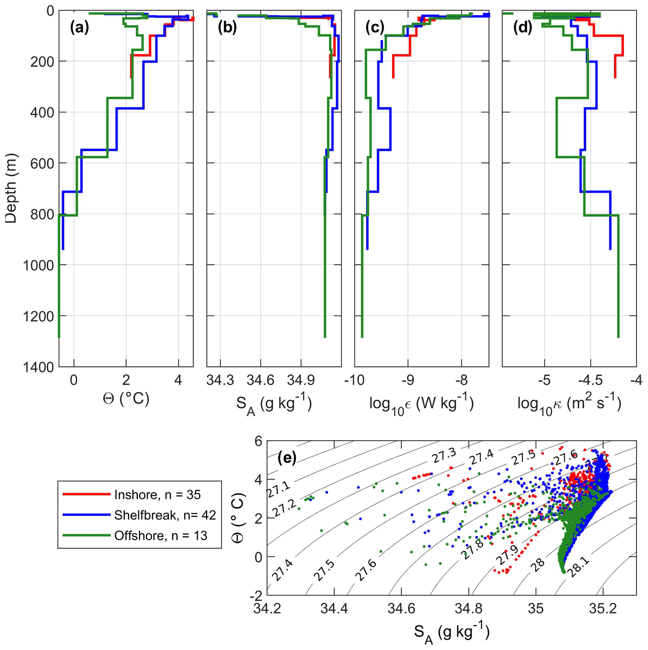
Figure 4Isopycnally averaged profiles of (a) Θ, (b) SA, (c) dissipation rate ϵ and (d) diapycnal diffusivity κ. The profiles are shown using the average depth of the isopycnals. (e) θ–SA diagram. Profiles are selected relative to the distance from the 800 m isobath: −10 km (red) inshore, at the shelf break in the Atlantic Water core (blue), and 10 km offshore (green). In the legend, n indicates the number of batch-averaged profiles used in each average.
3.3 Turbulence
On average, dissipation rates are the largest in the upper ocean, reaching 10−7 W kg−1 near the surface and decreasing rapidly with depth (Fig. 4c). In deeper layers, the dissipation rates are larger inshore than offshore, decreasing from W kg−1 in the shallows (red profiles) to 10−10 W kg−1 in the deep offshore profiles (green profiles). Between 400 and 600 m depth, a local maximum in the dissipation rate is observed in the core of the inflowing Atlantic Water current (blue profiles), where the strongest currents are observed (Kolås et al., 2020). Diffusivity is large in both the mixed layer and at depth close to the bottom (Fig. 4d), exceeding m2 s−1.
Of the microstructure measurements collected during the cruises, the process stations RS2 and P were analyzed and reported in detail in Fer et al. (2020b) and Koenig et al. (2020), respectively. The largest dissipation rates were measured at RS2, with high dissipation rates observed in the whole water column during a 6 h turbulent event (Fig. 3f), caused by an intense dissipation of lee waves driven by cross-slope tidal currents (Fer et al., 2020b). Process station P in the Nansen Basin far from the continental slope (Fig. 1) is a 24 h process study at a surface thermohaline front (Fig. 3g). At this specific station, turbulence structure in the mixed layer was generally consistent with turbulence production through convection by heat loss to the atmosphere and mechanical forcing by moderate wind (Koenig et al., 2020).
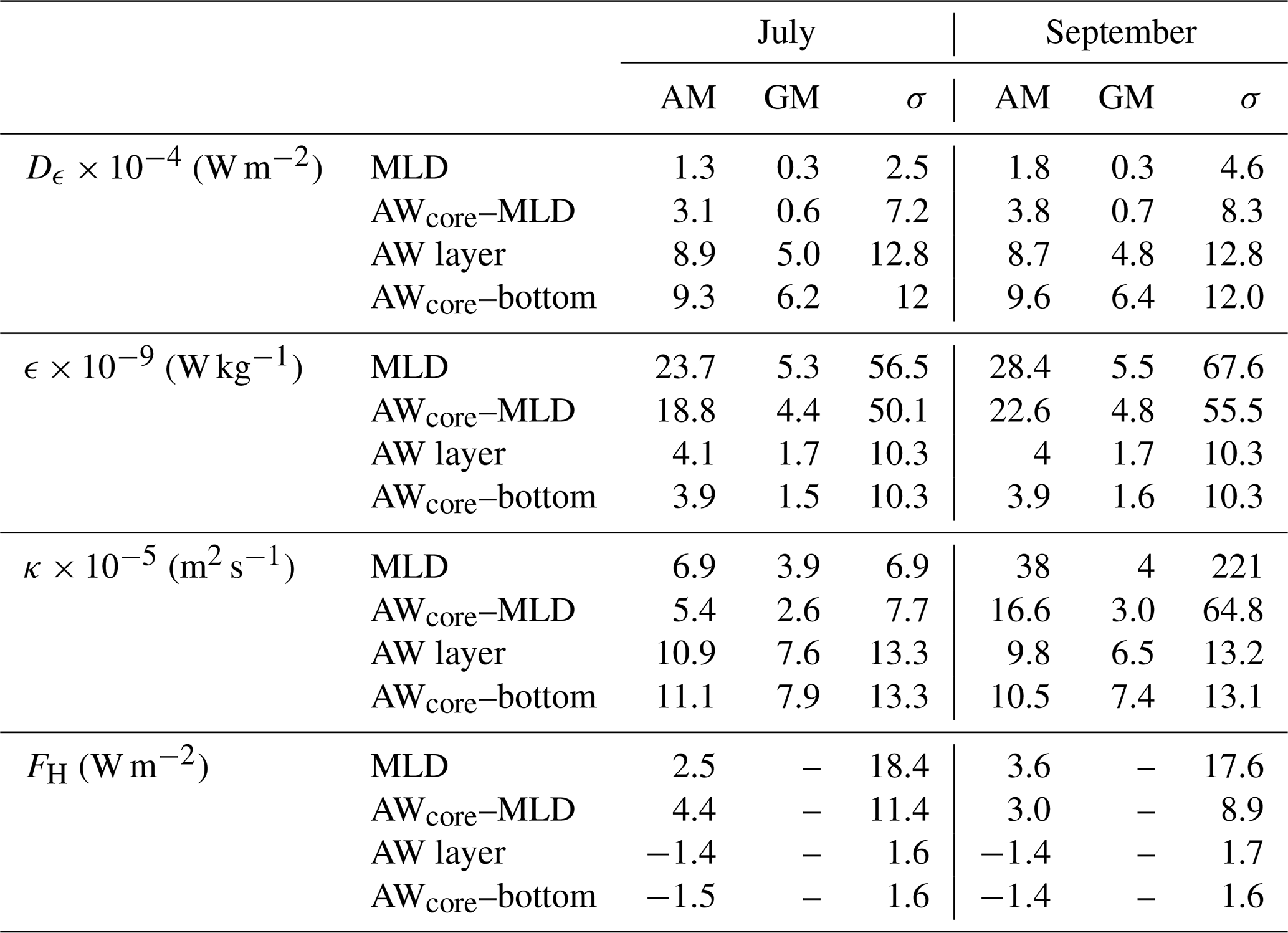
In the following sections, we will first examine the mixed layer evolution from summer to fall and the role of wind forcing. Then we will investigate the turbulence structure in the deeper layers, forced by tidal currents. Using the measurements in the Atlantic Water layer we quantify the vertical heat loss from the Atlantic Water layer. Basic statistics (arithmetic and geometric mean and standard deviations) of mixing parameters for July and September are summarized in Table 2. We used both arithmetic and geometric means to describe the dissipation rates, diffusivity and turbulent fluxes. For variables with lognormal distribution (such as ϵ and κ), the geometric mean (GM) characterizes the distribution's central tendency while the arithmetic mean (AM) tends to be disproportionately skewed by a small number of large values (Scheifele et al., 2020). AM characterizes the integrated effect of the distribution and is representative of the cumulative effect of mixing and average buoyancy transformations produced by mixing (Scheifele et al., 2020).
Table 2Statistics of the turbulence variables measured in July and September. AM: arithmetic mean; GM: geometric mean; σ: standard deviation; Dϵ: vertically integrated dissipation rate; ϵ: dissipation rate; κ: diffusivity; FH: vertical turbulent heat flux (positive upward). Four layers are defined. MLD: ±10 m around the base of the mixed layer; AWcore–MLD: from the Atlantic Water core to the mixed layer depth; AW layer: in the Atlantic Water layer; and AWcore–bottom: from the Atlantic Water core to the seafloor. The geometric mean is ill-defined for negative values and hence not provided for the turbulent heat fluxes.
4.1 Seasonal evolution
Solar heating melts the sea ice, which has consequences for the upper ocean dynamics. Throughout the summer, the mixed layer becomes fresher and lighter (34.9 g kg−1 and 27.7 kg m−3 in July, and 34 g kg−1 and 26.95 kg m−3 in September; Fig. 5) and also deepens (18 m in July and 23 m in September). This evolution in summer towards a lighter mixed layer is mainly due to the meltwater during the summer. In both summer and fall, dissipation rates, buoyancy fluxes and turbulent heat fluxes increased at the base and just below the mixed layer compared to the rest of the water column (Fig. 5 and Table 2).

Figure 5θ–SA diagrams where the color-coded bins are dissipation rate (a, d), turbulent heat flux (b, e) and magnitude of buoyancy flux (c, f; the buoyancy fluxes are all oriented downward). Contours are σ0, referenced to surface pressure. Panels (a), (b) and (c) are for summer (July cruise) and (d), (e) and (f) for fall (September cruise). The green star is the mean temperature and salinity property of the mixed layer in July and the purple circle is the corresponding value in September.
The depth-integrated dissipation rate at the base of the mixed layer Dml is on average about (1–2) × 10−4 W m−2 during both cruises, with a geometric mean of about W m−2 (Table 2). Turbulent buoyancy fluxes in the mixed layer are directed downward, and turbulent salt fluxes upward, in both July and September. Salt and buoyancy fluxes are larger in September than in July at the base of the mixed layer: the salt flux is kg s−1 m−2 in July and kg s−1 m−2 in September, and the buoyancy flux is W kg−1 in July and W kg−1 in September, as the meltwater content in the upper layer is larger in September than in July.
Turbulent heat fluxes across the base of the mixed layer are positive (upward) in both July and September, but larger in September than in July (3.6 and 2.5 W m−2 respectively). The turbulent heat fluxes measured during both cruises are comparable to what is observed under the sea ice in the absence of forcing events during the N-ICE2015 experiment (Meyer et al., 2017; Peterson et al., 2017) (about 2 W m−2), but about to times the heat fluxes (up to 100 W m−2) observed during storm events above the continental slope. Variations in the density field are dominated by the variations in salinity; thus buoyancy and salt fluxes vary concomitantly.
4.2 Wind forcing
Wind stress at the ocean surface is one of the main drivers for the upper layer turbulence and can increase the ocean-to-ice heat fluxes (Meyer et al., 2017; Dosser and Rainville, 2016). A fraction of the wind energy flux from the atmosphere to the ocean then fuels turbulence in the upper ocean and is dissipated in the mixed layer. Using the observed dissipation in the mixed layer and the wind energy input (Fig. 6), we obtain a line fit: , where Dml is the depth-integrated dissipation rate in the mixed layer. Observations in September are limited as only a few stations were performed with the VMP.
For relatively low values of E10 (less than W m−2), the relation is almost linear, suggesting that about 1 ‰ of wind energy input is dissipated in the mixed layer. For larger E10, additional processes such as breaking gravity waves can contribute. During the cruise in September, the surface waves were characterized by 0.5–1.5 m significant wave height (Sect. 3.1, Løken et al., 2019). Because the dissipation measurements are contaminated by the ship's wake in the upper 10 m, we cannot resolve the role of wave-boundary layer dynamics on the vertical structure of dissipation. Since the wave forcing in September was weak, we do not expect a substantial contribution to the observed nonlinear dependence of mixed-layer dissipation on wind energy input. However, the relatively large values of Dml in July when E10 was large (circles in Fig. 6) might be associated with surface waves.
The front process station P (green star) is more energetic than what is expected from only wind forcing as convection is active on the warm side of the front (Koenig et al., 2020). Dissipation in the mixed layer at RS2 (red circle) is only computed using the first casts as there is no data in the shallow mixed layer during the intense dissipation event driven by cross-slope tidal currents (Fig. 3f). The presence of sea ice in the region can also explain the nonlinearity of the relation between the wind energy and the energy dissipation in the mixed layer. Although the profiles were collected in ice-free conditions, some stations were close to the sea ice edge spotted from the ship.
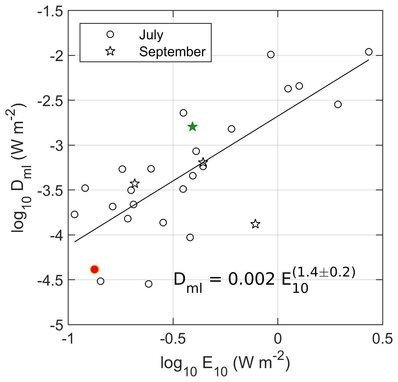
Figure 6Depth-integrated dissipation rate in the mixed layer, Dml, as a function of the wind energy input to the mixed layer, E10. Stars and circles are data from the September and July cruises, respectively. The red circle is the data point from the RS2 process station where nonlinear internal waves were observed (Fer et al., 2020b). The green star is the data point at the process station at a front in September where convection was also important (Koenig et al., 2020). The black line is the regression line, with the equation indicated. The uncertainty is the 95 % confidence interval.
Previous observations show that north of Svalbard is a region of substantial tidal mixing (Rippeth et al., 2015; Fer et al., 2015). The location is northward of the critical latitude of the main diurnal and semidiurnal tidal components (K1 and M2). The critical latitude, also called the turning latitude, is where the tidal frequency matches the local inertial frequency. The linear response at high latitudes is evanescent. The barotropic-to-baroclinic energy conversion from the tidal activity results in trapped linear waves that can only propagate along topography guidelines, or a nonlinear response with properties similar to lee waves (Vlasenko et al., 2003; Musgrave et al., 2016). A fraction of the energy in trapped waves or nonlinear waves will dissipate locally, leading to substantial vertical mixing (Padman and Dillon, 1991). In our observations, the dissipation rate below the mixed layer is typically low (Table 2), but energetic turbulence observed at some locations (Fig. 3) can be related to tidal forcing.
We select the profiles of turbulent heat fluxes and dissipation rates in categories of tidal current speed predicted from Arc5km2018 at the time of the measurement. Tidal current speed is defined as high (>5 cm s−1) or low (<5 cm s−1) (Fig. 7). The profiles in the corresponding categories are averaged with respect to height above bottom defined as the difference between the depth of the measurement and the seafloor depth. We obtained the average profiles as the maximum likelihood estimator from a lognormal distribution using the data points in 20 m vertical bins. The mixed layer was excluded in all the profiles to minimize the contribution from dissipation driven by surface processes.
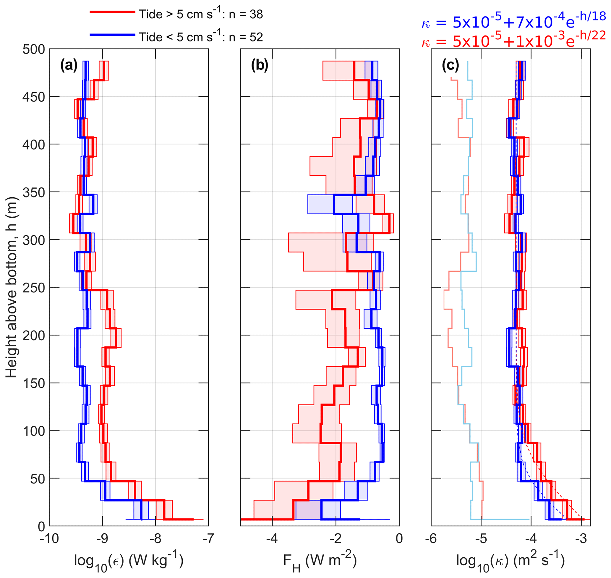
Figure 7Average profiles of (a) dissipation rate ϵ, (b) turbulent heat flux FH and (c) diapycnal diffusivity κ for small (blue) and large (red) tidal current amplitudes estimated from Arc5km2018 at the time and location of each station. Average profiles are obtained as the maximum likelihood estimator from a lognormal distribution using the data points in 20 m vertical bins. The vertical axis is height above bottom, relative to the seafloor depth from the echo sounder. n indicates the number of batch-averaged profiles for each tidal forcing category. Thin lines in (c) are the corresponding profiles for diffusivity at the lowest detection level (obtained by imposing a noise level for the dissipation rate of W kg−1). The dashed lines are the curve fits using an exponential function. Resulting equations with the best-fit coefficients are shown above the panel. The shading is the 95 % confidence envelope of the maximum likelihood.
From the seafloor to about 250 m height above bottom, the dissipation rate was larger ( W kg−1) in conditions with strong tidal currents compared to weaker tidal currents ( W kg−1). In both cases, the dissipation rate decreases quickly with height from the seafloor, down to dissipation rates of W kg−1 above 250 m from the bottom. The increase in dissipation rates for strong tidal forcing is associated with an absolute increase in the downward turbulent heat flux close to seafloor: −2.2 W m−2 when tidal currents were weak and about −3.2 W m−2 when tidal currents were strong.
Similar to the dissipation rate, the diapycnal diffusivity decreases with increasing height above bottom (Fig. 7c). Based on the observations from north of Svalbard, we can deduce an empirical relation that would allow an estimate of the diffusivity in conditions of strong (>5 cm s−1) or weak (<5 cm s−1) tidal currents. Following St. Laurent et al. (2002), we use a functional form for the diffusivity expressed as follows:
where κbg is a background diffusivity, κbot is the diffusivity value at the seafloor, h is the height above bottom and zdecay is the vertical decay scale of the diffusivity. We use m2 s−1, based on observations. Fitted equations for high and low tidal current speeds are shown above Fig. 7c. With large tidal amplitudes, κbot approximately doubles and the decay scale increases from 18 to 22 m (95 % confidence interval of 2 m).
We investigate the role of two distinct contributions from tidal currents to the turbulent mixing. While tidally driven processes may lead to interior mixing away from the seabed (Fer et al., 2020b), bottom stress from barotropic tidal currents must be balanced by dissipation in bottom boundary layers. The tidal work can be representative of the barotropic-to-baroclinic conversion and can be related to the dissipation of propagating or trapped internal wave energy, which can likely extend far into the water column. In the bottom boundary layer, the bottom stress from the barotropic tide also plays a role. The relative contributions to mixing through the tidal work and the tidally driven bottom drag are unknown.
We analyze the vertically integrated dissipation rate in the bottom 250 m of the water column D250 (and below the surface mixed layer) separately with respect to tidal work and the tidally driven bottom drag (Fig. 8). The total rate of work by barotropic tidal currents interacting with topography was computed as the product of the Baines force (Baines, 1982) and the barotropically induced vertical velocity following Nash et al. (2006), for the main diurnal and semidiurnal constituents. D250 does not correlate well with the tidal work, Wtidal, at the time of observations (not shown). A least-squares power-law fit results in an uncertainty of the power which is more than 50 % of its estimated value: .
The tidally driven bottom drag is examined next, expressed as in Jayne and St. Laurent (2001):
where Cd is the bottom drag coefficient, ρ0 is the seawater density and u is the tidal current vector. Note that this equation is analogous to the drag relation for the wind energy flux E10 (in Sect. 4.2). In calculations two different tidal currents are used: the instantaneous tidal speed ut at the time and location of each station and a statistical estimate of the representative cross-isobath tidal current, urms, at the location of each station (Fig. 8). Both are obtained from the Arc5km2018 model. We calculated urms from the predicted local cross-isobath component of the tidal currents over an arbitrary 30 d window using all constituents; this choice offers a parameter easily available for parameterization purposes, independent of observations.
In analyzing the vertically integrated dissipation rates with respect to local forcing at the time of observations (Fig. 8a), we averaged the process stations in batches as explained in Sect. 3; this allows for including some time variability in the observations. For the analysis of typical tidal forcing, we averaged each process station as one data point because each location is associated with a time-independent urms (Fig. 8b). The local bottom drag at the time of observations correlates well with D250 and follows the power-law fit with a considerable scatter (uncertainty of the power is less than 25 % its estimated value; Fig. 8a). This nonlinear relationship between D250 (dissipation in the bottom 250 m) and Wbotdrag shows parallels with the nonlinear relationship between Dml (dissipation in the surface mixed layer) and E10. If we force a linear relation in panel (a), we find a drag coefficient of . This value is comparable to but smaller than the typical range of bottom drag values of (1–3) × 10−3 and the bottom drag deduced from in situ observations in Bering Strait of (Couto et al., 2020). The red data points in Fig. 8 are from the station RS2, where energetic turbulence was observed from dissipation of nonlinear internal waves (Fer et al., 2020b). It partly explains why larger dissipation rates are observed here than what could be expected from the tidally driven bottom drag alone. The analysis is repeated using the bottom drag parameters calculated using the typical cross-isobath tidal forcing urms (Fig. 8b). The scatter is reduced, and in particular the bottom-drag relation offers a useful parameterization to infer vertically integrated dissipation rates. An estimate along the margin of the Eurasian basin will be given in the discussion using the relation in Fig. 8b.
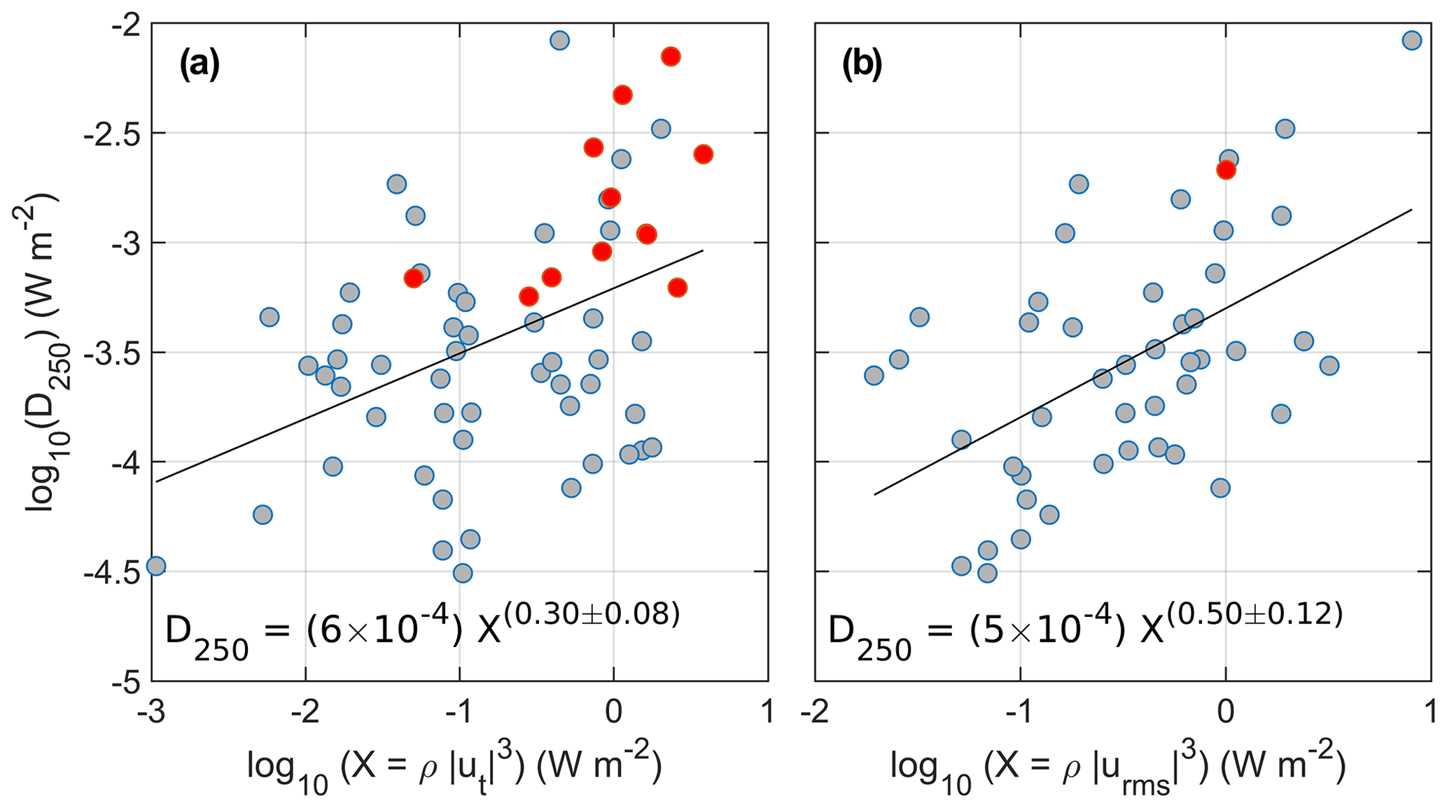
Figure 8Depth-integrated dissipation rate in the bottom 250 m (D250) regressed against (a) the instantaneous tidally driven bottom drag and (b) the typical tidally driven bottom drag (using urms). See text for details. Linear fits on the logarithmic parameter space (i.e., power-law fits) denoted by the black lines, and the corresponding equations are indicated with the 95 % confidence levels. Red dots are the data points from the RS2 station. Process stations are batch-averaged (in sets of 4–5 consecutive profiles) in (a) and averaged over the station duration in (b).
As the heat content in the Atlantic Water in the Arctic Ocean has the potential to melt the sea ice cover completely, it is important to quantify the turbulent dissipation rates and heat fluxes out of the Atlantic Water in the new conditions of a warming Arctic. The depth-integrated dissipation rate from the base of the mixed layer to the Atlantic Water core is about W m−2, and the average dissipation rate is about W kg−1, almost as large as what is observed in the mixed layer (Table 2). We estimated the vertical turbulent heat flux between the upper limit of the Atlantic Water layer and the mixed layer depth (Fig. 9a), in both summer and fall. The maximum positive heat flux (upward toward the surface) is observed near the 800 m isobath, reaching up to 30 W m−2 in July and 10 W m−2 in September. This isobath is representative of the average location of the core of Atlantic Water (Kolås et al., 2020). Outside the Atlantic Water boundary current, about 20 km inshore and offshore from the 800 m isobath, vertical turbulent heat fluxes are negligible, with a maximum of 5 W m−2. In July, the Atlantic Water core tends to be closer to the base of the mixed layer compared to September (Fig. 9a), implying that the heat contained in the Atlantic Water is more likely to reach the surface in July than in September. Meltwater in September enhances the stratification near the surface and isolates the Atlantic Water layer from the mixed layer. At some stations, vertical turbulent heat fluxes are negative (0 to −5 W m−2), directed downward from the surface toward the Atlantic Water layer. The negative fluxes are mainly found near the core of the Atlantic Water inflow. These negative heat fluxes are observed when warm water reaches the surface, and the temperature increases from the top of the Atlantic Water layer up to the surface. This situation is typical of summer conditions north of Svalbard where the Atlantic Water extends close to the surface and the cold halocline is absent (Polyakov et al., 2017).
The lateral (cross-isobath) distribution of the diapycnal heat fluxes is similar in July and September (Fig. 9a). We therefore used all data points to fit a Gaussian curve (Fig. 9b), with an aim to estimate the integrated heat loss from the Atlantic Water layer. Between −20 and +20 km, the heat loss due to vertical turbulent heat fluxes is about 1.2×10⁵ W m−1. Using independent hydrographic observations but covering the same observational time period, Kolås et al. (2020) found that the average along-path change of heat content from section B to E was about 9.1×10⁷ W m−1, and about 9.6×10⁶ W m−1 from section C to D, corresponding to an average heat loss of about 500 W m−2 north of Svalbard. Heat loss from the Atlantic Water layer by vertical turbulent heat fluxes to the upper ocean then accounts for only about 1 % of the total Atlantic Water heat loss north of Svalbard. This estimate can be biased low since during the period of measurements wind forcing was weak to moderate with low variability. Processes that contribute to the turbulent heat loss of the Atlantic Water layer are discussed in Sect. 7.
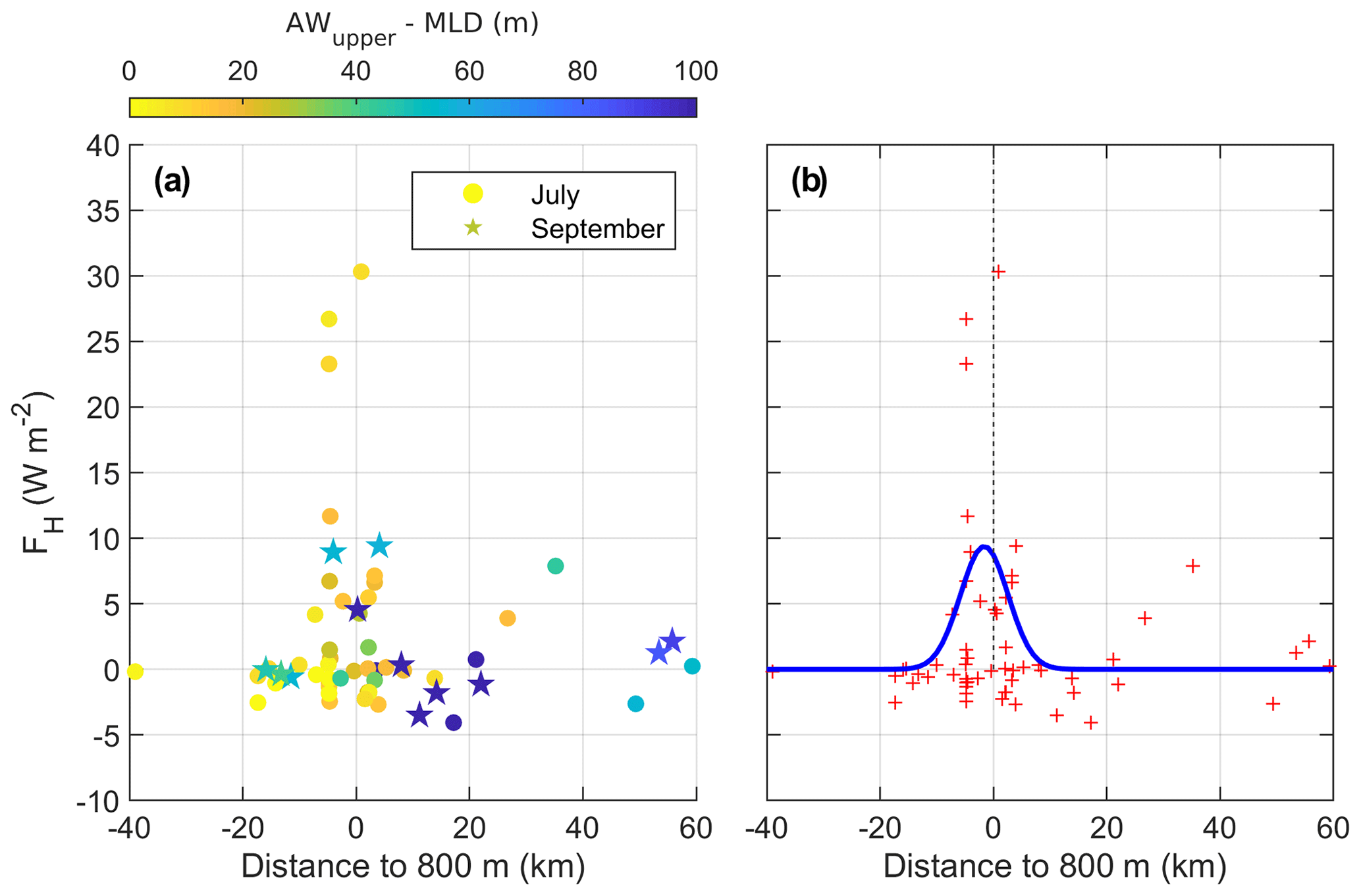
Figure 9(a) Lateral distribution of the mean vertical turbulent heat flux from the AW upper boundary to the base of the mixed layer. The horizontal axis is the horizontal distance to the 800 m isobath. The color code is the vertical distance between the upper boundary of the Atlantic Water layer and the mixed layer depth. Markers identify the stations collected in July (circles) and September (stars). (b) A Gaussian fit (blue line) to the vertical turbulent heat flux from the Atlantic Water to the mixed layer depth (red crosses).
7.1 Estimates of the tidally driven dissipation rate in the Eurasian Basin
Turbulent mixing in the Arctic is not well-documented, and measurements close to the bottom are scarce. The bottom drag estimated from the Arc5km2018 predictions in the Arctic Ocean, using a constant drag coefficient, is larger on the shelf and on the ridges than in the deep basin (not shown), as a result of sensitivity to the strength of the barotropic tidal current. These areas coincide with regions of enhanced tidal activity in the Arctic (Padman and Erofeeva, 2004). Using this tidally driven bottom drag and the relation inferred from the data collected north of Svalbard (Sect. 5 and equation in Fig. 8b), we estimate the depth-integrated dissipation rate. The highest bottom depth-integrated dissipation rates in the Arctic are found on the shelves and are consistent with the pan-Arctic observations compiled and presented in Rippeth et al. (2015), reaching 10−3 W m−2 (not shown).
Because the parameterization is obtained using a limited dataset from a localized region north of Svalbard, instead of presenting Arctic-wide maps we concentrate on the Eurasian Basin from north of Svalbard into the East Siberian Sea. The cross-isobath tidal currents along this transect, particularly in the Laptev Sea, are strong (see Fig. 1 of Fer et al., 2020b). Figure 10 shows the time-averaged cross-isobath tidal current amplitude, and the depth-integrated dissipation rate in the bottom 250 m estimated using the equation in Fig. 8b, along the continental slope of the Eurasian basin. The largest tidal speeds are observed north of Svalbard and in the eastern part of the Laptev Sea where the slope connects to the Lomonosov Ridge, reaching more than 0.1 m s−1 (Fig. 10a). The largest average bottom dissipation rates across the continental slope are observed at 35∘ E, just east of Svalbard and at the Lomonosov Ridge, reaching W m−2. We present two estimates for the dissipation: the vertically integrated dissipation rate in the bottom 250 m, D250, averaged laterally between the 400 and 1200 m isobaths (blue line and left axis; Fig. 10b), and D250 integrated meridionally between the 400 and 1200 m isobaths (red line and right axis; Fig. 10b). This volume-integrated dissipation rate, per unit meter along the shelf break, shows variations similar to the averaged D250, except at 70∘ E. This is the location of the Santa Anna Trough, where the Atlantic Water from the Barents Sea flows into the Arctic Ocean and where the distance between the 400 and 1200 m isobaths triples compared to the rest of the Eurasian continental slope. Rippeth et al. (2015) argued, based on microstructure measurements and tidal velocities from the TPXO8 inverse solution, that the energy supporting much of the enhanced dissipation along the continental slopes in the Eurasian Basin, and more specifically north of Svalbard and around the Lomonosov Ridge, is of tidal origin. The mean-integrated dissipation over the Atlantic layer observed in Rippeth et al. (2015) is of a similar order of magnitude to the depth-integrated dissipation in the bottom 250 m deduced from the tidally driven bottom drag as observed in our study. However, the bottom depth-integrated dissipation rate extrapolated from a local relation valid north of Svalbard to the Arctic Ocean must be considered with caution.
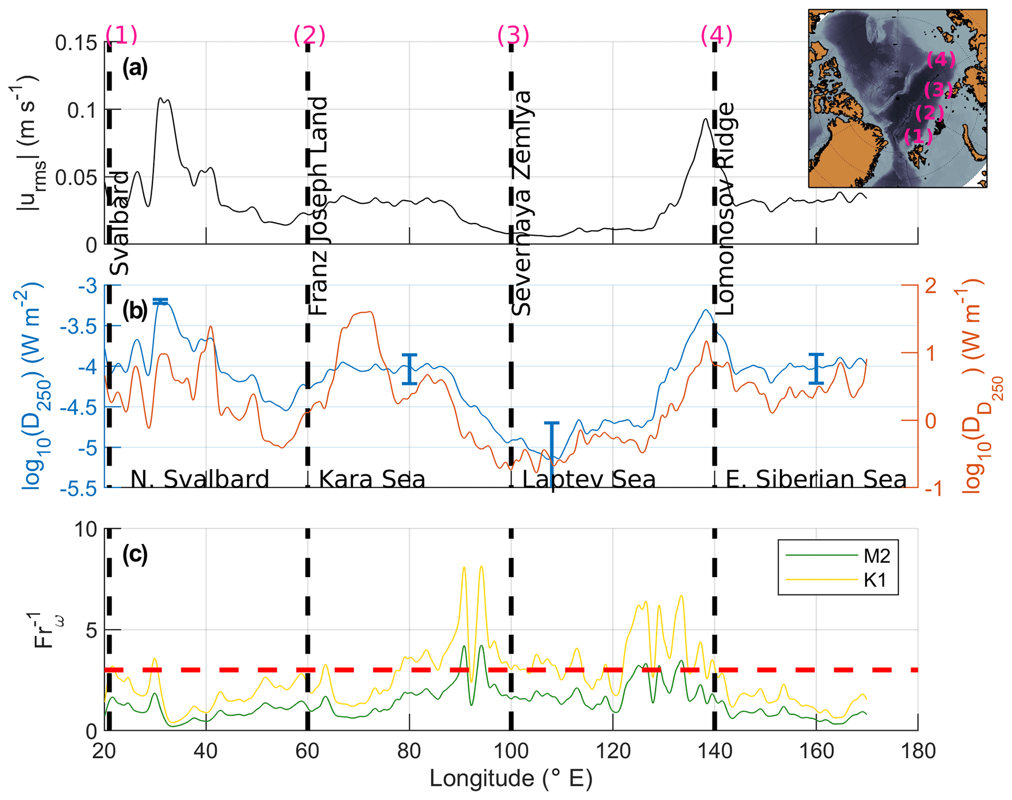
Figure 10(a) Typical cross-isobath tidal speed along the Eurasian continental slope obtained from Arc5km2018 and averaged meridionally between the 400 and 1200 m isobaths. (b) Left axis: the depth-integrated dissipation rate in the bottom 250 m, D250, calculated from the tidally driven bottom drag using the relation in Fig. 8b, averaged between the 400 and 1200 m isobaths. The blue vertical bars, shown at selected locations for clarity, are the error bars from the uncertainty on the equation in Fig. 8b. Right axis: D250 integrated laterally between the 400 and 1200 m isobaths. (c) Inverse Froude number for both the semidiurnal M2 (green) and the diurnal K1 tidal components (yellow). The red dashed line is , a threshold for the development of nonlinear processes (Legg and Klymak, 2008).
As the Eurasian Arctic is poleward of the critical latitude for most of the main tidal constituents, the response to tidal flow over sloping topography can be nonlinear when the topographic obstruction of the stratified flow is large. Legg and Klymak (2008) proposed that an inverse Froude number, , based on a vertical excursion distance of the tidal current over bottom slope, can be used to estimate the possibility of occurrence of highly nonlinear jump-like lee waves, such as those observed at station RS2 (Fer et al., 2020b) or modeled over the Spitsbergen Bank (Rippeth et al., 2017), a shallow bank south of Svalbard and poleward of the M2 critical latitude. The inverse Froude number is expressed as follows:
where is the bottom slope and ω is the tidal frequency. In our calculations we used the Brunt–Väisälä frequency N near the bottom, extracted from the MIMOC climatology in August (the result is not sensitive to this choice as the near-bottom stratification does not have a strong seasonal cycle). When , the vertical excursion distance induced by tidal currents is sufficiently large that hydraulic jumps could occur and nonlinear waves can develop (Legg and Klymak, 2008). The calculations along the Eurasian shelf break are presented in Fig. 10c for the semidiurnal and the diurnal tidal forcing. Along the Eurasian slope, we expect nonlinear internal waves to develop for the diurnal tidal forcing in the eastern part of the Kara and Laptev seas, where is much larger than 3, the threshold value for the development of nonlinear processes. Values slightly above this threshold are also observed north of Svalbard. In the region north of Svalbard and in the eastern part of the Laptev Sea, the large depth-integrated dissipation rate observed in Fig. 10b can be driven by nonlinear waves implied by the peaks of (Fig. 10c). These two areas warrant further studies. In the eastern part of the Kara Sea, however, the depth-integrated dissipation rates are relatively low despite the large inverse Froude number values that suggest nonlinear processes could develop there.
North of Svalbard, observations of nonlinear internal waves were documented in Fer et al. (2020b) during the July cruise at RS2. They showed abrupt isopycnal vertical displacements of 10–50 m and an intense dissipation associated with cross-isobath diurnal tidal currents of ∼0.15 m s−1. The dissipation of these nonlinear internal waves creates an increase in dissipation in the whole water column by a factor of 100 and turbulent heat fluxes are about 15 W m−2 compared with the background turbulent heat flux of 1 W m−2 (Fer et al., 2020b). The increase in the dissipation rate driven by these nonlinear waves is also noticeable in Fig. 8a and c (the red dots). At this location, the inverse Froude number for the diurnal frequency exceeds 3, supporting the interpretation that such conditions can favor the development of nonlinear processes.
7.2 Atlantic Water heat loss
The Atlantic Water loses heat as it propagates cyclonically along the continental slope in the Arctic Ocean. Around the Yermak Plateau, the along-path cooling and freshening are estimated to be 0.2 ∘C per 100 km and 0.01 g kg−1 per 100 km, corresponding to a surface heat flux between 400 and 500 W m−2 (Boyd and D'Asaro, 1994; Cokelet et al., 2008; Kolås and Fer, 2018). We found that the upward heat loss from turbulent heat fluxes from the Atlantic Water layer up to the mixed layer reached on average 8 W m−2. This figure is 1 order of magnitude larger than vertical heat flux from the Atlantic Water to the surface in the Laptev Sea (on the order of 0.1–1 W m−2, Polyakov et al., 2019). North of Svalbard and in the Laptev Sea, heat loss due to turbulent vertical mixing represents less than 10 % of the total heat loss of the Atlantic Water (Kolås et al., 2020; Polyakov et al., 2019).
Ivanov and Timokhov (2019) estimated that from the Yermak Plateau to the Lomonosov Ridge, 41 % of the Atlantic Water heat is lost to atmosphere, 31 % to deep ocean and 20 % is lost laterally. Heat loss resulting from vertical heat fluxes contributes to the heat loss to the atmosphere and to the deep ocean, but not to the lateral heat loss. Several processes can lead to lateral heat loss north of Svalbard, including eddy spreading from the slope into the basin (Crews et al., 2018; Våge et al., 2016). Using eddy-resolving regional model results, Crews et al. (2018) found that eddies export 1.0 TW out of the boundary current, delivering heat into the interior Arctic Ocean at an average rate of ∼15 W m−2. West of Svalbard, Kolås and Fer (2018) found that the measured turbulent heat flux in the WSC was too small to account for the cooling rate of the Atlantic Water layer but reported a substantial contribution from energetic convective mixing of an unstable bottom boundary layer on the slope. Convection was driven by the Ekman advection of buoyant water across the slope and complements the turbulent mixing in the cooling process. The estimated lateral buoyancy flux was about 10−8 W kg−1 (Kolås and Fer, 2018), sufficient to maintain a large fraction of the observed dissipation rates, and corresponds to a heat flux of approximately 40 W m−2. We can expect similar processes to extract heat and salt from the Atlantic Water core north of Svalbard. Such processes can explain why turbulent heat fluxes are only responsible for 10 % of the Atlantic heat loss north of Svalbard. Furthermore, large heat loss during extreme events should not be ignored. For example, Meyer et al. (2017) found that the average heat flux of about 7 W m−2 across the 0 ∘C isotherm increased during storms, exceeding 30 W m−2. During our survey, without extreme wind events, the turbulent heat fluxes represent only a small portion of the heat loss of the Atlantic Water.
We reported on observations of turbulence north of Svalbard, collected during two cruises in summer and fall 2018, in conditions with varying tidal forcing and weak to moderate wind forcing with low variability. We describe the observed structure of dissipation rates and vertical mixing in the region and identify the main processing supplying energy for turbulence. This dataset complements the scarce observations and offers further insight into turbulent mixing processes in the Arctic Ocean.
During the observation period, from July to September, the surface meltwater content increases. Averaged across the base of the mixed layer, salt and buoyancy fluxes more than double from summer to fall, although the vertically integrated dissipation rate in the mixed layer (Dml) remains similar. Variability of the turbulent dissipation in the mixed layer varies nonlinearly with the energy input from the wind E10, approximated by . The scatter is large, however, from turbulence produced in the mixed layer by other processes such as convection.
In the deeper part of the water column, tidal forcing appears to be one of the main sources of mixing. When the tidal current amplitude exceeds 5 cm s−1, near-bottom dissipation rates and diapycnal diffusivity double. The vertical decay scale of the diffusivity is 22 m for those strong tidal currents, compared to 18 m for weaker tidal currents; the bottom diffusivity is larger with strong tidal currents than for weaker ones ( and m2 s−1, respectively). The variability of the vertically integrated dissipation rate in the bottommost 250 m, D250, can be approximated by bottom stress from the barotropic tidal current, parameterized using a quadratic bottom drag. Using a statistical estimate of the typical cross-isobath tidal currents, regression of D250 against the tidally driven bottom drag Wbotdrag gives . The average bottom drag coefficient north of Svalbard is estimated to be about . Applying the power-law fit to tidal currents along the Eurasian continental slope, we find that turbulence is enhanced north of Svalbard and east of the Laptev Sea above the Lomonosov ridge, with D250 reaching W m−2. Higher above the seafloor, the dissipation rates can also increase as a result of breaking nonlinear internal waves driven by tidal currents. A Froude-number-based calculation suggests that nonlinear response and internal hydraulic jumps are expected to develop north of Svalbard, in the Kara and Laptev seas. The generalization of our results to the Eurasian Basin should however be considered with caution as it is based on an empirical relation extrapolated from north of Svalbard. More in situ observations from different sites in the Eurasian Basin and elsewhere in the Arctic are needed to confirm our results.
The Atlantic Water layer north of Svalbard cools and freshens by mixing with the surrounding waters. Across the warm Atlantic Water boundary current, heat loss due to vertical turbulent fluxes from the top of the Atlantic Water layer to the mixed layer is the largest above the 800 m isobath, reaching ∼30 W m−2, corresponding to the location of the boundary current core. In our dataset, the average heat loss from the Atlantic Water layer due to vertical mixing is about 8 W m−2 and accounts for only about 1 % of the estimated total heat loss of the Atlantic Water layer. Increased vertical mixing during storms would add to this figure. However, integrated studies addressing lateral mixing processes and frontal systems as well as extreme conditions such as storms are needed to close the heat budget in this region.
All data are available from the Norwegian Marine Data Centre; datasets from the July cruise (KB 2018616) are available at https://doi.org/10.21335/NMDC-2047975397 (Fer et al., 2019), and datasets from the September cruise (KH 2018709) are available at https://doi.org/10.21335/NMDC-2039932526 (Fer et al., 2020a).
ZK drafted the paper. All the authors collected, processed and analyzed the observations and edited and commented on the paper.
Ilker Fer is a member of the editorial board of Ocean Science, but other than that the authors declare no competing interests.
This work was supported by the Nansen Legacy Project, project number 276730. We thank the officers, crew and scientists of the R/V Kronprins Haakon cruise in September 2018 and of the R/V Kristine Bonnevie cruise in July 2018. Comments from two reviewers helped improve an earlier version of the paper.
This research has been supported by the Norges Forskningsråd (grant no. 276730).
This paper was edited by Bernadette Sloyan and reviewed by two anonymous referees.
Årthun, M., Eldevik, T., Smedsrud, L., Skagseth, Ø., and Ingvaldsen, R.: Quantifying the influence of Atlantic heat on Barents Sea ice variability and retreat, J. Climate, 25, 4736–4743, https://doi.org/10.1175/JCLI-D-11-00466.1, 2012. a, b
Baines, P. G.: On internal tide generation models, Deep-Sea Res. Pt. A, 29, 307–338, https://doi.org/10.1016/0198-0149(82)90098-X, 1982. a
Bouffard, D. and Boegman, L.: A diapycnal diffusivity model for stratified environmental flows, Dynam. Atmos. Oceans, 61, 14–34, https://doi.org/10.1016/j.dynatmoce.2013.02.002, 2013. a
Boyd, T. J. and D'Asaro, E. A.: Cooling of the West Spitsbergen Current: Wintertime observations west of Svalbard, J. Geophys. Res., 99, 22597–22618, https://doi.org/10.1029/94JC01824, 1994. a
Cokelet, E. D., Tervalon, N., and Bellingham, J. G.: Hydrography of the West Spitsbergen Current, Svalbard Branch: Autumn 2001, J. Geophys. Res., 113, C01006, https://doi.org/10.1029/2007JC004150, 2008. a, b, c
Couto, N., Alford, M. H., MacKinnon, J., and Mickett, J. B.: Mixing rates and bottom drag in Bering Strait, J. Phys. Oceanogr., 50, 809–825, https://doi.org/10.1175/JPO-D-19-0154.1, 2020. a
Crews, L., Sundfjord, A., Albretsen, J., and Hattermann, T.: Mesoscale Eddy Activity and Transport in the Atlantic Water Inflow Region North of Svalbard, J. Geophys. Res., 123, 201–215, https://doi.org/10.1002/2017JC013198, 2018. a, b, c
Crews, L., Sundfjord, A., and Hattermann, T.: How the Yermak Pass Branch Regulates Atlantic Water Inflow to the Arctic Ocean, J. Geophys. Res.-Oceans, 124, 267–280, https://doi.org/10.1029/2018JC014476, 2019. a
Dosser, H. V. and Rainville, L.: Dynamics of the changing near-inertial internal wave field in the Arctic Ocean, J. Phys. Oceanogr., 46, 395–415, https://doi.org/10.1175/jpo-d-15-0056.1, 2016. a
Duarte, P., Sundfjord, A., Meyer, A., Hudson, S. R., Spreen, G., and Smedsrud, L. H.: Warm Atlantic water explains observed sea ice melt rates north of Svalbard, J. Geophys. Res.-Oceans, 125, e2019JC015662, https://doi.org/10.1029/2019JC015662, 2020. a
Erofeeva, S. and Egbert, G.: Arc5km2018: Arctic Ocean Inverse Tide Model on a 5 kilometer grid, 2018, Dataset, Arctic Data Center, https://doi.org/10.18739/A21R6N14K, 2020. a
Fer, I.: Weak vertical diffusion allows maintenance of cold halocline in the central Arctic, Atmos. Ocean. Sci. Lett., 2, 148–152, https://doi.org/10.1080/16742834.2009.11446789, 2009. a, b
Fer, I., Müller, M., and Peterson, A. K.: Tidal forcing, energetics, and mixing near the Yermak Plateau, Ocean Sci., 11, 287–304, https://doi.org/10.5194/os-11-287-2015, 2015. a, b, c
Fer, I., Koenig, Z., Kolås, E., Falck, E., Fossum, T., Ludvigsen, M., Marnela, M., Nilsen, F., Norgren, P., and Skogseth, R.: Physical oceanography data from the cruise KH 2018709 with R.V. Kronprins Haakon, 12–24 September 2018, Data Set, Norwegian Marine Data Center (NMDC), https://doi.org/10.21335/NMDC-2039932526, 2019. a, b
Fer, I., Koenig, Z., Bosse, A., Falck, E., Kolås, E., and Nilsen, F.: Physical oceanography data from the cruise KB 2018616 with R.V. Kristine Bonnevie, Data Set, Norwegian Marine Data Center (NMDC), https://doi.org/10.21335/NMDC-2047975397, 2020a. a, b
Fer, I., Koenig, Z., Kozlov, I. E., Ostrowski, M., Rippeth, T. P., Padman, L., Bosse, A., and Kolås, E.: Tidally forced lee waves drive turbulent mixing along the Arctic Ocean margins, Geophys. Res. Lett., 47, e2020GL088083, https://doi.org/10.1029/2020GL088083, 2020b. a, b, c, d, e, f, g, h, i, j
Gregg, M., D'Asaro, E., Riley, J., and Kunze, E.: Mixing efficiency in the ocean, Annu. Rev. Mar. Sci., 10, 443–473, https://doi.org/10.1146/annurev-marine-121916-063643, 2018. a
Guarino, M.-V., Sime, L. C., Schröeder, D., Malmierca-Vallet, I., Rosenblum, E., Ringer, M., Ridley, J., Feltham, D., Bitz, C., Steig, E. J., Wolff, E., Stroeve, J., and Sellar, A.: Sea-ice-free Arctic during the Last Interglacial supports fast future loss, Nat. Clim. Change, 10, 928–932, https://doi.org/10.1038/s41558-020-0865-2, 2020. a
Ivanov, V., Alexeev, V., Koldunov, N. V., Repina, I., Sandø, A. B., Smedsrud, L. H., and Smirnov, A.: Arctic Ocean heat impact on regional ice decay: A suggested positive feedback, J. Phys. Oceanogr., 46, 1437–1456, https://doi.org/10.1175/JPO-D-15-0144.1, 2016. a
Jakobsson, M., Mayer, L., Coakley, B., Dowdeswell, J. A., Forbes, S., Fridman, B., Hodnesdal, H., Noormets, R., Pedersen, R., Rebesco, M., Schenke, H. W., Zarayskaya, Y., Accettella, D., Armstrong, A., Anderson, R. M., Bienhoff, P., Camerlenghi, A., Church, I., Edwards, M., Gardner, J. V., Hall, J. K., Hell, B., Hestvik, O., Kristoffersen, Y., Marcussen, C., Mohammad, R., Mosher, D., Nghiem, S. V., Pedrosa, M. T., Travaglini, P. G., and Weatherall, P.: The International Bathymetric Chart of the Arctic Ocean (IBCAO) Version 3.0, Geophys. Res. Lett., 39, L12609, https://doi.org/10.1029/2012gl052219, 2012. a, b
Jayne, S. and St. Laurent, L.: Parameterizing tidal dissipation over rough topography, Geophys. Res. Lett., 28, 811–814, https://doi.org/10.1029/2000GL012044, 2001. a
Koenig, Z., Provost, C., Sennechael, N., Garric, G., and Gascard, J.-C.: The Yermak Pass Branch: A Major Pathway for the Atlantic Water North of Svalbard?, J. Geophys. Res., 122, 9332–9349, https://doi.org/10.1002/2017JC013271, 2017. a
Koenig, Z., Fer, I., Kolås, E., Fossum, T., Norgren, P., and Ludvigsen, M.: Observations of turbulence at a near-surface temperature front in the Arctic Ocean, J. Geophys. Res.-Oceans, 125, e2019JC015526, https://doi.org/10.1029/2019JC015526, 2020. a, b, c, d
Kolås, E. and Fer, I.: Hydrography, transport and mixing of the West Spitsbergen Current: the Svalbard Branch in summer 2015, Ocean Sci., 14, 1603–1618, https://doi.org/10.5194/os-14-1603-2018, 2018. a, b, c
Kolås, E. H., Koenig, Z., Fer, I., Nilsen, F., and Marnela, M.: Structure and transport of Atlantic Water north of Svalbard from observations in summer and fall 2018, J. Geophys. Res.-Oceans, 125, e2020JC016174, https://doi.org/10.1029/2020JC016174, 2020. a, b, c, d, e, f, g, h
Krishfield, R. A. and Perovich, D. K.: Spatial and temporal variability of oceanic heat flux to the Arctic ice pack, J. Geophys. Res., 110, C07021, https://doi.org/10.1029/2004JC002293, 2005. a
Large, W. and Pond, S.: Open ocean momentum flux measurements in moderate to strong winds, J. Phys. Oceanogr., 11, 324–336, https://doi.org/10.1175/1520-0485(1981)011<0324:OOMFMI>2.0.CO;2, 1981. a
Legg, S. and Klymak, J.: Internal hydraulic jumps and overturning generated by tidal flow over a tall steep ridge, J. Phys. Oceanogr., 38, 1949–1964, https://doi.org/10.1175/2008JPO3777.1, 2008. a, b, c
Lenn, Y.-D., Rippeth, T. P., Old, C. P., Bacon, S., Polyakov, I., Ivanov, V., and Hölemann, J.: Intermittent Intense turbulent mixing under Ice in the Laptev Sea continental shelf, J. Phys. Oceanogr., 41, 531–547, https://doi.org/10.1175/2010JPO4425.1, 2011. a
Lincoln, B. J., Rippeth, T. P., Lenn, Y.-D., Timmermans, M. L., Williams, W. J., and Bacon, S.: Wind-driven mixing at intermediate depths in an ice-free Arctic Ocean, Geophys. Res. Lett., 43, 9749–9756, https://doi.org/10.1002/2016GL070454, 2016. a, b
Løken, T. K., Rabault, J., Jensen, A., Sutherland, G., Christensen, K. H., and Müller, M.: Wave measurements from ship mounted sensors in the Arctic marginal ice zone, arXiv preprint, arXiv:1911.07612, 2019. a, b
Maykut, G. A. and McPhee, M. G.: Solar heating of the Arctic mixed layer, J. Geophys. Res., 100, 24691–24703, https://doi.org/10.1029/95JC02554, 1995. a
Maykut, G. A. and Untersteiner, N.: Some results from a time-dependent thermodynamic model of sea ice, J. Geophys. Res., 76, 1550–1575, https://doi.org/10.1029/JC076i006p01550, 1971. a
McDougall, J. and Barker, P.: Getting started with TEOS-10 and the Gibbs Seawater (GSW) Oceanographic Toolbox, 28 pp., SCOR/IAPSO WG127, ISBN 978-0-646-55621-5, 2011. a
Menze, S., Ingvaldsen, R. B., Haugan, P., Fer, I., Sundfjord, A., Beszczynska-Moeller, A., and Falk-Petersen, S.: Atlantic Water Pathways Along the North-Western Svalbard Shelf Mapped Using Vessel-Mounted Current Profilers, J. Geophys. Res.-Oceans, 124, 1699–1716, https://doi.org/10.1029/2018JC014299, 2019. a
Meyer, A., Fer, I., Sundfjord, A., and Peterson, A. K.: Mixing rates and vertical heat fluxes north of Svalbard from Arctic winter to spring, J. Geophys. Res., 122, 4569–4586, https://doi.org/10.1002/2016JC012441, 2017. a, b, c, d
Musgrave, R. C., MacKinnon, J. A., Pinkel, R., Waterhouse, A. F., and Nash, J.: Tidally Driven Processes Leading to Near-Field Turbulence in a Channel at the Crest of the Mendocino Escarpment, J. Phys. Oceanogr., 46, 1137–1155, https://doi.org/10.1175/Jpo-D-15-0021.1, 2016. a
Nash, J. D., Kunze, E., Lee, C. M., and Sanford, T. B.: Structure of the baroclinic tide generated at Kaena Ridge, Hawaii, J. Phys. Oceanogr., 36, 1123–1135, https://doi.org/10.1175/JPO2883.1, 2006. a
Nasmyth, P.: Ocean turbulence, PhD thesis, The University of British Columbia, 1970. a
Oakey, N. S. and Elliott, A. J.: Dissipation within the surface mixed layer, J. Phys. Oceanogr., 12, 171–185, https://doi.org/10.1175/1520-0485(1982)012<0171:DWTSML>2.0.CO;2, 1982. a
Osborn, T. R.: Estimates of the local rate of vertical diffusion from dissipation measurements, J. Phys. Oceanogr., 10, 83–89, 1980. a
Padman, L. and Dillon, T. M.: Turbulent mixing near the Yermak Plateau during the coordinated Eastern Arctic Experiment, J. Geophys. Res.-Oceans, 96, 4769–4782, https://doi.org/10.1029/90JC02260, 1991. a, b
Padman, L. and Erofeeva, S.: A barotropic inverse tidal model for the Arctic Ocean, Geophys. Res. Lett., 31, L02303, https://doi.org/10.1029/2003GL019003, 2004. a
Padman, L., Plueddemann, A. J., Muench, R. D., and Pinkel, R.: Diurnal tides near the Yermak Plateau, J. Geophys. Res., 97, 12639–12652, https://doi.org/10.1029/92JC01097, 1992. a
Peterson, A. K., Fer, I., McPhee, M. G., and Randelhoff, A.: Turbulent heat and momentum fluxes in the upper ocean under Arctic sea ice, J. Geophys. Res.-Oceans, 122, 1–18, https://doi.org/10.1002/2016JC012283, 2017. a, b
Polyakov, I. V., Pnyushkov, A. V., Alkire, M. B., Ashik, I. M., Baumann, T. M., Carmack, E. C., Goszczko, I., Guthrie, J., Ivanov, V. V., Kanzow, T., Krishfield, R., Kwok, R., Sundfjord, A., Morison, J., Rember, R., and Yulin, A.: Greater role for Atlantic inflows on sea-ice loss in the Eurasian Basin of the Arctic Ocean, Science, 356, 285–291, https://doi.org/10.1126/science.aai8204, 2017. a, b
Polyakov, I. V., Padman, L., Lenn, Y. D., Pnyushkov, A., Rember, R., and Ivanov, V. V.: Eastern Arctic Ocean Diapycnal Heat Fluxes through Large Double-Diffusive Steps, J. Phys. Oceanogr., 49, 227–246, https://doi.org/10.1175/Jpo-D-18-0080.1, 2019. a, b
Polyakov, I. V., Rippeth, T. P., Fer, I., Alkire, M. B., Baumann, T. M., Carmack, E. C., Ingvaldsen, R., Ivanov, V. V., Janout, M., Lind, S., et al.: Weakening of cold halocline layer exposes sea ice to oceanic heat in the eastern Arctic Ocean, J. Climate, 33, 8107–8123, https://doi.org/10.1175/JCLI-D-19-0976.1, 2020. a, b, c
Rainville, L. and Woodgate, R. A.: Observations of internal wave generation in the seasonally ice-free Arctic, Geophys. Res. Lett., 36, L23604, https://doi.org/10.1029/2009GL041291, 2009. a
Randelhoff, A., Fer, I., and Sundfjord, A.: Turbulent upper-ocean mixing affected by meltwater layers during Arctic summer, J. Phys. Oceanogr., 47, 835–853, https://doi.org/10.1175/JPO-D-16-0200.1, 2017. a
Rippeth, T. P., Lincoln, B. J., Lenn, Y.-D., Green, J. A. M., Sundfjord, A., and Bacon, S.: Tide-mediated warming of Arctic halocline by Atlantic heat fluxes over rough topography, Nat. Geosci., 8, 191–194, https://doi.org/10.1038/ngeo2350, 2015. a, b, c, d, e, f, g
Rippeth, T. P., Vlasenko, V., Stashchuk, N., Scannell, B. D., Green, J. A. M., Lincoln, B. J., and Bacon, S.: Tidal Conversion and Mixing Poleward of the Critical Latitude (an Arctic Case Study), Geophys. Res. Lett., 44, 12349–12357, https://doi.org/10.1002/2017gl075310, 2017. a, b
Rudels, B., Meyer, R., Fahrbach, E., Ivanov, V., Østerhus, S., Quadfasel, D., Schauer, U., Tverberg, V., and Woodgate, R.: Water mass distribution in Fram Strait and over the Yermak Plateau in summer 1997, Annales Geophysicae, 18, 687–705, https://doi.org/10.1007/s00585-000-0687-5, 2000. a
Scheifele, B., Waterman, S., and Carpenter, J.: Turbulence and Mixing in the Arctic Ocean's Amundsen Gulf, J. Phys. Oceanogr., 51, 169–186, 2020. a, b
Schmidtko, S., Johnson, G. C., and Lyman, J. M.: MIMOC: A global monthly isopycnal upper-ocean climatology with mixed layers, J. Geophys. Res.-Oceans, 118, 1658–1672, https://doi.org/10.1002/jgrc.20122, 2013. a
St. Laurent, L. C., Simmons, H. L., and Jayne, S. R.: Estimating tidally driven mixing in the deep ocean, Geophys. Res. Lett., 29, 2106, https://doi.org/10.1029/2002GL015633, 2002. a
Timmermans, M.-L. and Marshall, J.: Understanding Arctic Ocean Circulation: A Review of Ocean Dynamics in a Changing Climate, J. Geophys. Res.-Oceans, 125, e2018JC014378, https://doi.org/10.1029/2018JC014378, 2020. a
Tsubouchi, T., Bacon, S., Aksenov, Y., Naveira Garabato, A. C., Beszczynska-Möller, A., Hansen, E., De Steur, L., Curry, B., and Lee, C. M.: The Arctic Ocean seasonal cycles of heat and freshwater fluxes: Observation-based inverse estimates, J. Phys. Oceanogr., 48, 2029–2055, https://doi.org/10.1175/JPO-D-17-0239.1, 2018. a
Vlasenko, V., Stashchuk, N., Hutter, K., and Sabinin, K.: Nonlinear internal waves forced by tides near the critical latitude, Deep-Sea Res. Pt. I, 50, 317–338, https://doi.org/10.1016/S0967-0637(03)00018-9, 2003. a
Våge, K., Pickart, R. S., Pavlov, V., Lin, P., Torres, D. J., Ingvaldsen, R., Sundfjord, A., and Proshutinsky, A.: The Atlantic Water boundary current in the Nansen Basin: Transport and mechanisms of lateral exchange, J. Geophys. Res.-Oceans, 121, 6946–6960, https://doi.org/10.1002/2016JC011715, 2016. a, b