Nutrient ratios driven by vertical stratification regulate phytoplankton community structure in the oligotrophic western Pacific Ocean

The stratification of the upper oligotrophic ocean has a direct impact on biogeochemistry by regulating the components of the upper-ocean environment that are critical to biological productivity, such as light availability for photosynthesis and nutrient supply from the deep ocean. We investigated the spatial distribution pattern and diversity of phytoplankton communities in the western Pacific Ocean (WPO) in the autumn of 2016, 2017, and 2018. Our results showed the phytoplankton community structure mainly consisted of cyanobacteria, diatoms, and dinoflagellates, while the abundance of Chrysophyceae was negligible. Phytoplankton abundance was high from the equatorial region to 10^∘ N and decreased with increasing latitude in spatial distribution. Phytoplankton also showed a strong variation in the vertical distribution. The potential influences of physicochemical parameters on phytoplankton abundance were analyzed by a structural equation model (SEM) to determine nutrient ratios driven by vertical stratification to regulate phytoplankton community structure in the typical oligotrophic ocean. Regions with strong vertical stratification were more favorable for cyanobacteria, whereas weak vertical stratification was more conducive to diatoms and dinoflagellates. Our study shows that stratification is a major determinant of phytoplankton community structure and highlights that physical processes in the ocean control phytoplankton community structure by driving the balance of chemical elements, providing a database to better predict models of changes in phytoplankton community structure under future ocean scenarios.

1 Introduction

Phytoplankton contribute nearly half of global primary production (Field et al., 1998) and represent an important part of biogeochemical cycling and transformation (Falkowski et al., 1998). Marine phytoplankton link the cycling of different elements through their demand for multiple nutrients such as nitrogen (N), phosphorus (P), or iron and their relative availability (Hillebrand et al., 2013). The Redfield ratio is probably the most powerful generalization and cornerstone of the marine biogeochemical cycle (Redfield et al., 1963; Schindler, 2003). The nutrient requirements of phytoplankton are limited by the environmental conditions in which they grow, and nutrient limitation increases the N : P ratio of primary production (Carlson, 2002; Fogg, 1983; Karl et al., 1998). Nitrogen fixation by phytoplankton may deplete phosphorus from the upper ocean, causing an increase to the N : P ratios (Karl et al., 2001). The photosynthesis does not cease, even when there are not enough nutrients to grow (Bertilsson et al., 2003; Geider et al., 1998; Goldman et al., 1979).

Upper-ocean stratification plays an important role in the climate system and in many marine biogeochemical processes. The degree of vertical mixing is controlled by the strength of near-surface density stratification (Cronin et al., 2013; Qiu et al., 2004), which impacts the formation of the surface mixed layer (ML) and the entrainment process at the ML's base. The ML depth directly modulates the oceanic reaction to atmospheric forcing and the ocean ventilation process that includes the sinking of water masses into the ocean interior, accompanied by heat, carbon, and oxygen. Upper-ocean stratification can directly affect important processes such as biogeochemistry and primary production by regulating the light supply for photosynthesis and nutrient supply from the subsurface ocean (Yamaguchi et al., 2019). While the strengthened stratification may produce better light availability for the phytoplankton community, it will also prevent vertical nutrient supply to the euphotic zone from the deep sea (Doney, 2006). Previous studies have shown that net primary production (NPP) shows a stronger linear decrease with stronger vertical stratification and a significant decrease in surface nitrate and phosphate concentrations. The decrease in NPP can be partly explained by the increase in vertical stratification that leads to changes in nutrient concentration (Yamaguchi et al., 2019).

In the present study, we focused on the vertical structure of the change in the ocean temperature and salinity, i.e., the change in the density stratification. The vertical stratification index (VSI) used in this study is the potential density difference between the surface layer and the depth of 200 m (Δρ200), which can quantify the strength of the upper-ocean stratification well (Mena et al., 2019). The purpose of this study is to determine the community composition mechanisms that drive phytoplankton in the oligotrophic region. These mechanisms are related to vertical stratification and nutrient ratios. We explored how vertical stratification affects the composition of phytoplankton communities. We hypothesized that vertical stratification might regulate phytoplankton abundance and community composition by driving the ratio of nutrients.

2 Materials and methods

2.1 Study area and sampling

This study relied on the shared voyage of the western Pacific Ocean (WPO; 0–20^∘ N, 120–130^∘ E), commissioned by the National Natural Science Foundation of China. Physical, biological, chemical, and geological surveys were carried out from September to November in 2016, 2017, and 2018 aboard the R/V Kexue. The sampling stations used in this study are shown in Fig. 1; the sampling layers were 5, 25, 50, 75, 100, 150, and 200 m. Phytoplankton samples from different water layers were placed in 1 L polyethylene bottles, fixed in formaldehyde solution (3 %), and stored in the dark. Nutrient samples from different layers were placed in PE bottles, frozen, and stored at −20^∘ for laboratory nutrient analysis.

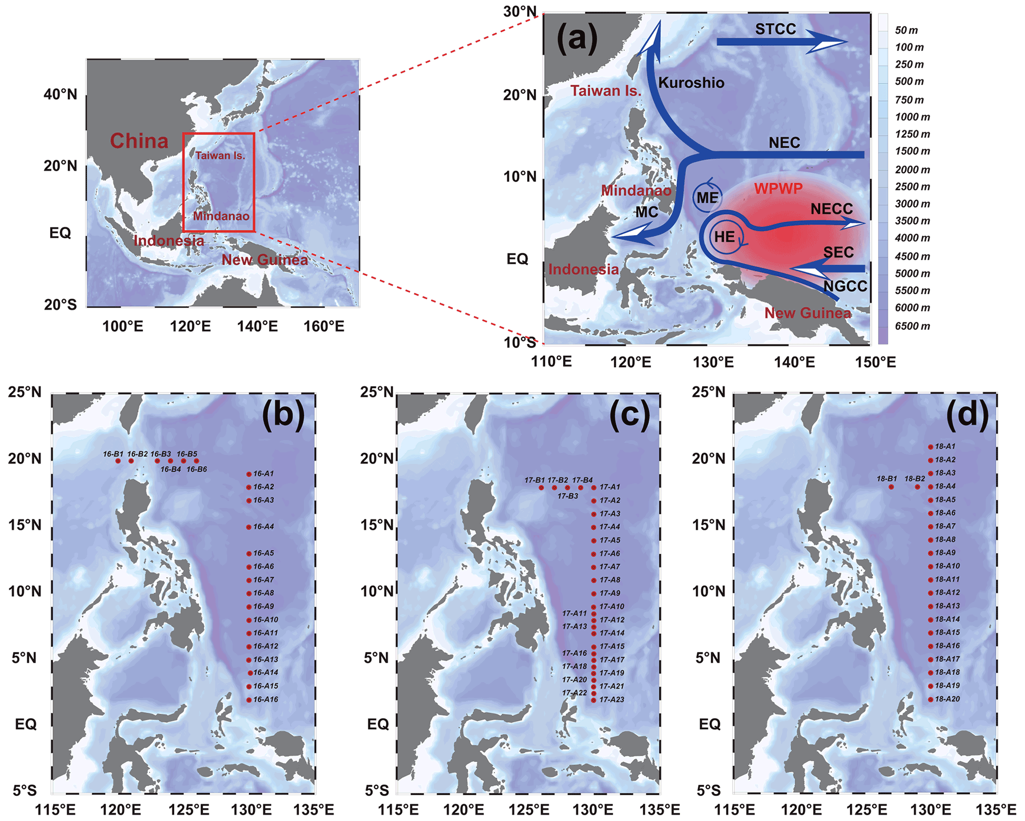
Figure 1 Stations in the western Pacific Ocean (WPO) of three cruises. (a) Current systems of the WPO; (b, c, d) sampling stations of the 2016, 2017, and 2018 cruises, respectively. The station at 130^∘ E forms section A, and the station at 20^∘ N forms section B. Map of the WPO shows the major geographic names and the surface currents, including the Subtropical Counter Current (STCC), the North Equatorial Current (NEC), the North Equatorial Counter Current (NECC), the South Equatorial Current (SEC), the New Guinea Coastal Current (NGCC), the Mindanao Current (MC), the Mindanao Eddy (ME), and the Halmahera Eddy (HE).

2.2 Identification of phytoplankton

After returning to the laboratory, the Utermöhl method was applied for phytoplankton analysis. A 1 L subsample was allowed to stand for 48 h, after which 800 mL supernatant was removed carefully by siphoning through a catheter, taking care to prevent the catheter from touching the bottom of the bottle. Thereafter, the remaining 200 mL of liquid was gently mixed and half of it was further concentrated with a 100 mL sedimentation column (Utermöhl method) for 48 h sedimentation (Sun et al., 2002). The phytoplankton species were identified and enumerated under an inverted microscope (AE2000, Motic, Xiamen, China) at 400× (or 200×) magnification. Phytoplankton identification was conducted as described by Jin and Chen (1965), Yamaji (1991), and Sun and Liu (2002), and the World Register of Marine Species (http://www.marinespecies.org, last access: 12 May 2020). Species identification was as close as possible to the species level. The minimum size of the organisms identified and counted is 20 µm.

2.3 Laboratory nutrient analysis

The Technicon AA3 Auto-Analyzer (Bran + Luebbe, Norderstedt, Germany) based on classical colorimetric methods was used for the analysis and determination of nutrients (Grasshoff et al., 2009). Soluble inorganic phosphorus (PO₄-P) was determined by the phosphomolybdenum blue method with a limit of detection of 0.02 µmol L⁻¹, dissolved silicate (SiO₃-Si) was determined by the silicon molybdenum blue method with a limit of detection of 0.02 µmol L⁻¹, nitrate (NO₃-N) was determined by the cadmium column method with a limit of detection of 0.01 µmol L⁻¹, nitrite (NO₂-N) was determined by the naphthalene ethylenediamine method with a limit of detection of 0.01 µmol L⁻¹ (Dai et al., 2008), and ammonia (NH₄-N) was determined by the sodium salicylate method with a limit of detection of 0.03 µmol L⁻¹ (Guo et al., 2014; Pai et al., 2001). The nitrogen-to-phosphorous (N : P) ratio was calculated by dividing nitrogen concentration (NO${}_{\mathrm{3}}^{-}$ + NO${}_{\mathrm{2}}^{-}$) by phosphate concentration.

2.4 Analysis and methods

A SBE911 conductivity, temperature, and depth (CTD) sensor and standard Sea-Bird Electronics methods were used to process recorded hydrological parameters. The depth of the mixed layer (ML) is calculated as follows:

$$\left(S,T\right)=\left(S_{\mathrm{ref}},T_{\mathrm{ref}}-\mathrm{\Delta }T\right),$$

where S and T are the salinity and temperature, respectively, and S_ref and T_ref are the temperature and salinity at 5 m; ΔT is equal to 0.5 ^∘C.

We calculated the vertical stratification index (VSI) to indicate the degree of vertical stratification of the water column:

$$\mathrm{VSI}=\mathrm{\Sigma }\left[{\mathit{\delta }}_{\mathit{\theta }}\right(m+\mathrm{1})-{\mathit{\delta }}_{\mathit{\theta }}(m\left)\right],$$

where δ_θ is the potential density anomaly and m is the depth from 5 to 200 m.

The abundance of phytoplankton cells in the water column was calculated through the trapezoidal integral method (Zhu et al., 2019):

$$P=\left\{\sum _{i=\mathrm{1}}^{n-\mathrm{1}}{\displaystyle \frac{P_{i+\mathrm{1}}+P_i}{\mathrm{2}}}\left(D_{i+\mathrm{1}}-D_i\right)\right\}/\left(D_n-D_{\mathrm{1}}\right),$$

where P is the average value of phytoplankton abundance in water column, P_i is the abundance value of phytoplankton in layer i, i+1 is the layer i+1, D_n is the maximum sampling depth, D_i is the depth of layer i, and n is the sampling level.

We clustered all species based on Bray–Curtis similarity distance over the 3 years, and the results showed four distinct regions using the primer (version 6). Distance-based redundancy analysis (db-RDA) and principal co-ordinates analysis (PCoA) were performed using the R package vegan (version 2.5-7) (Oksanen et al., 2020) to explain the relationship between environmental parameters, i.e., temperature, salinity, depth, VSI, dissolved inorganic nitrogen (DIN), dissolved inorganic phosphorus (DIP), and dissolved silicate (DSi), and phytoplankton community structure. The results were visualized using the R package ggplot2 (version 3.3.2). A structural equation model (SEM) was used to assess the relative direct and indirect impact of physical and chemical parameters on phytoplankton abundance. The chi-square test (χ²), comparative fit index (CFI), and goodness-of-fit index (GFI) were used to assess the model fit.

3 Results

3.1 Hydrographic features of the study area during the sampling years

The surface temperature and salinity of the surveyed sea area in 2016, 2017, and 2018 are shown in Fig. 2. In general, the temperature increased with decreasing latitude, and the stations near the Equator exhibited the highest temperature; in contrast, the salinity showed an opposite trend to that of temperature, with a high value from 15 to 20^∘ N. The surface temperature (Fig. 2) of the surveyed area in 2016 ranged from 28.58 ^∘C (station 16-B1) to 30.14 ^∘C (station 16-A16), with an average of 29.43 ^∘C. The surface salinity (Fig. 2) of the surveyed area in 2016 ranged from 33.80 (station 16-B2) to 34.65 (station 16-A2), with an average of 34.32. The surface temperature (Fig. 2) of the surveyed area in 2017 ranged from 27.91 ^∘C (station 17-A4) to 30.19 ^∘C (station 17-A20), with an average of 29.26 ^∘C. The surface salinity (Fig. 2) of the surveyed area in 2017 ranged from 33.38 (station 17-A16) to 34.64 (station 17-B4), with an average of 33.94. The surface temperature (Fig. 2) of the surveyed sea area in 2018 ranged from 26.33 ^∘C (station 18-B1) to 29.79 ^∘C (station 18-A17), with an average of 28.83 ^∘C. The surface salinity (Fig. 2) of the surveyed sea area in 2018 ranged from 33.77 (station 18-A14) to 34.64 (station 18-B1), with an average of 34.21.

The profile distribution of temperature and salinity based on the cross-sectional data of different water layers at each station obtained from the survey is shown in Fig. 2. The temperature of the shallow-water column (0–100 m) is higher than that of the deep-water column (100–200 m). The salinity values of the deep-water bodies (100–200 m) were higher than those of the shallow-water bodies (0–100 m). The values of temperature and salinity in 2016, 2017, and 2018 did not change significantly. The temperature of the section in 2016 ranged from 12.16 ^∘C (200 m at station 16-A11) to 30.14 ^∘C (5 m at station 16-A16), with an average of 25.74 ^∘C. The salinity of the section in 2016 ranged from 33.80 (5 m at station 16-B2) to 35.39 (150 m at station 16-A16), with an average of 34.61 ^∘C. The temperature of the section in 2017 ranged from 11.16 ^∘C (200 m at station 17-A13) to 30.19 ^∘C (5 m at station 17-A20), with an average of 25.18 ^∘C. The salinity of the section in 2017 ranged from 33.38 (5 m at station 17-A16) to 35.24 (150 m at station 17-A23), with an average of 34.46. The temperature of the section in 2018 ranged from 9.65 ^∘C (200 m at station 18-A14) to 29.79 ^∘C (5 m at station 18-A17), with an average of 24.22 ^∘C. The salinity of the section in 2018 ranged from 33.77 ^∘C (5 m at station 18-A14) to 35.39 ^∘C (150 m at station 18-A17), with an average of 34.57.

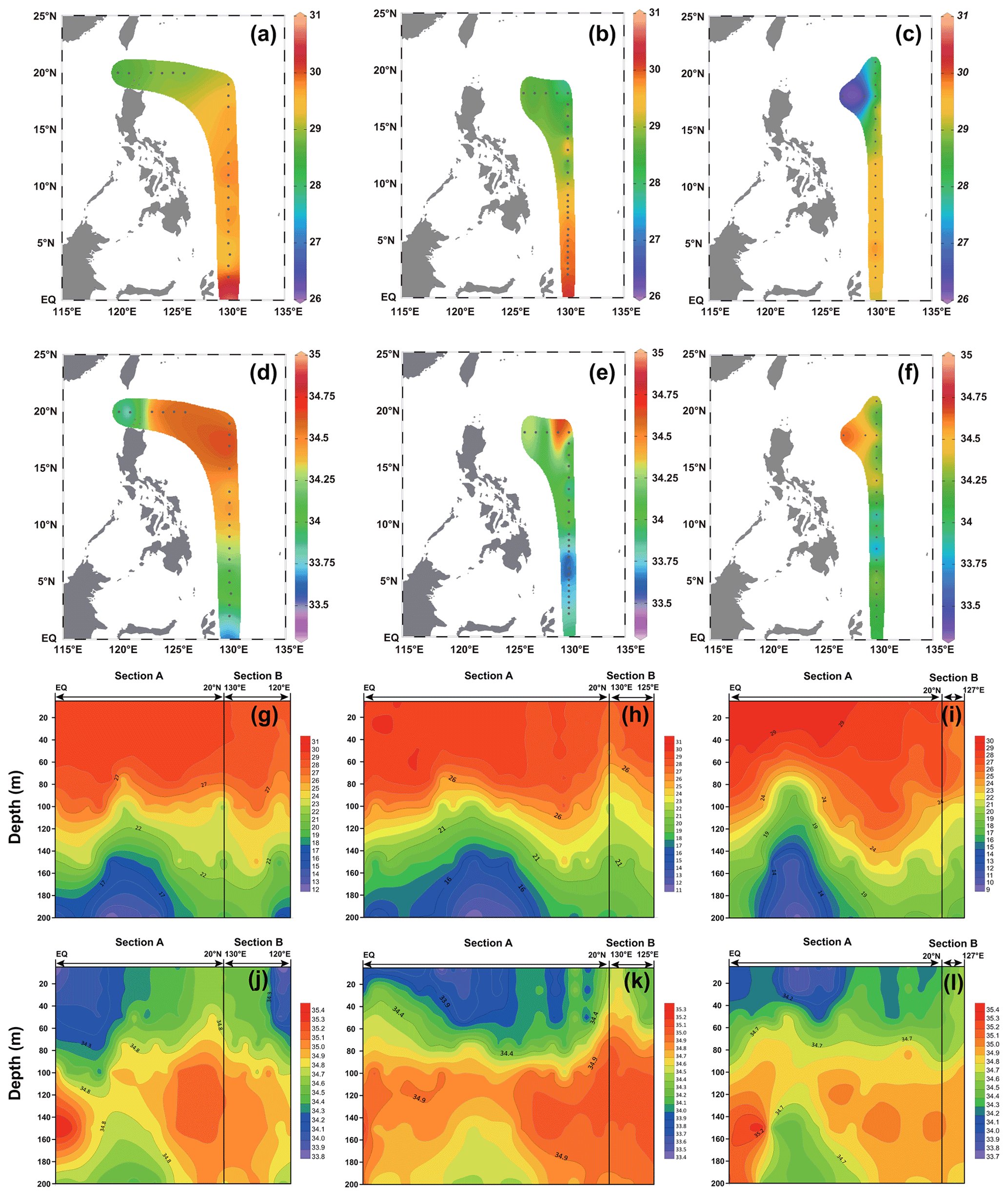
Figure 2 The temperature and salinity distribution in the WPO from three cruises. (a–c) Surface temperature in 2016, 2017, and 2018, respectively; (d–f) surface salinity in 2016, 2017, and 2018, respectively; (g–i) vertical distribution of temperature in 2016, 2017, and 2018, respectively; and (j–l) vertical distribution of salinity in 2016, 2017, and 2018, respectively.

The distribution of the VSI in latitude for the three cruises is shown in Fig. 3. Overall, the VSI showed a similar distribution pattern in the three cruises, with the highest value occurring at 7–8^∘ N and a decreasing trend with increasing latitude. In the 2016 cruise (Fig. 3a), the minimum value of VSI (2.54) appeared in the station at 20^∘ N (station 16-B4), and the maximum value (4.94) appeared in the station at 7^∘ N (station 16-A11), with an average of 3.90±0.76. In the 2017 cruise (Fig. 3b), a minimum value of VSI (2.85) appeared in the station at 18^∘ N (station 17-B4), and the maximum value (5.54) appeared in the station at 7^∘ N (station 17-A14), with an average of 4.30±0.82. In the 2018 cruise (Fig. 3c), the minimum value of VSI (2.50) occurred in the station at 18^∘ N (station 18-B1), and the maximum value (5.48) occurred in the station at 8^∘ N (station 18-A14), with an average of 4.01±0.95. Interestingly, the VSI varied significantly across latitudinal regions; the VSI was high from the Equator to 10^∘ N, while it was low at 10–20^∘ N.

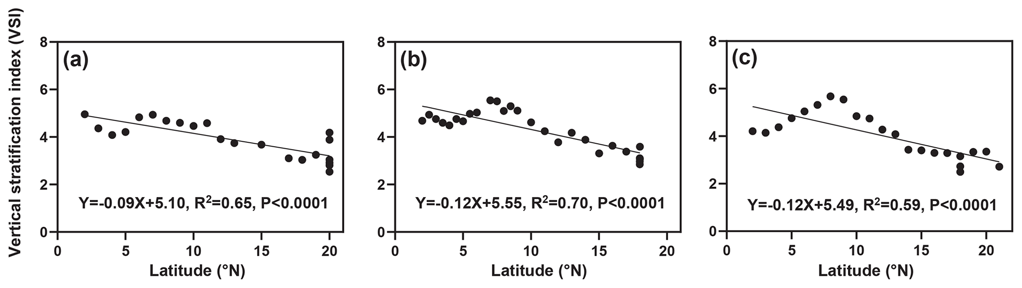
Figure 3 Linear fits of the vertical stratification index with latitude (a) in 2016, (b) 2017, and (c) 2018. The black dots are the VSI of each station.

3.2 Interannual variation of phytoplankton communities

Figure 4a, b, and c show the horizontal distribution of surface phytoplankton abundance from 2016 to 2018. The interannual variation in phytoplankton was relatively stable, and the sampling area and sampling time from 2016 to 2018 were generally consistent. Most phytoplankton species varied little from year to year in their distribution. Phytoplankton distribution showed a trend of decreasing abundance from the Equator to the north with a minor abundance peak at about 10^∘ N. This abundance peak was associated with the predominance of Trichodesmium. However, affected by coastal currents, high-abundance patches dominated by diatoms were also observed in the Luzon Strait area south of Taiwan, which were carried to the surface by upwelling currents and accounted for more than 67.76 % of the abundance at this station. Relatively high abundances were observed at stations in the Kuroshio Current extension region, consisting mainly of cosmopolitan and warm-water species. Phytoplankton abundance was the lowest in the high-latitude region.

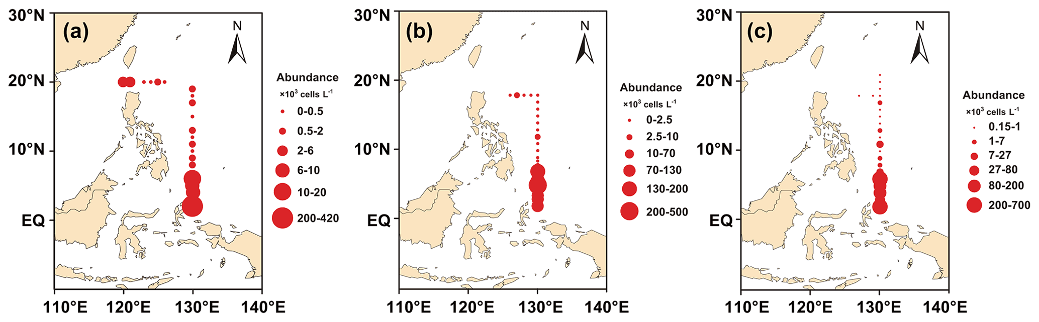
Figure 4 Horizontal distribution of phytoplankton abundance in the WPO: (a) surface layer in 2016, (b) surface layer in 2017, and (c) surface layer in 2018.

3.3 Vertical distribution of phytoplankton abundance

Figure 5 shows the vertical distribution of the phytoplankton. The overall trend in the WPO was consistent across the three cruises in 2016 (Fig. 5a), 2017 (Fig. 5b), and 2018 (Fig. 5c), with the phytoplankton distribution showing variations with latitude and differences in vertical distribution at depth. In terms of latitude, high-phytoplankton-value areas were concentrated near the Equator (0–8^∘ E). Vertical distribution of phytoplankton indicated that the plankton-abundant areas occurred from 0–50 m, and the phytoplankton abundance gradually decreased with the increase in depth. Vertical distribution of phytoplankton abundance differed significantly across different areas. In the areas near the Equator affected by the Halmahera Eddy (HE) and Mindanao Eddy (ME), phytoplankton abundance was mainly concentrated in the upper water column (0–50 m) and consisted mainly of cyanobacteria. In the northern area affected by the Kuroshio Current, the lower phytoplankton abundance was mostly dominated by the equatorial stations, while the phytoplankton species composition was mostly dominated by diatoms and dinoflagellates.

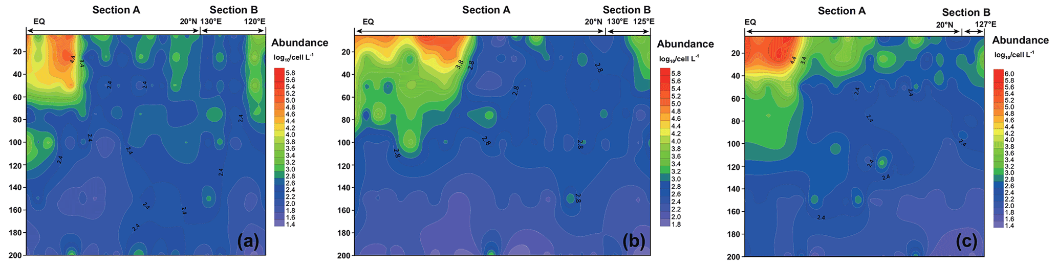
Figure 5 Vertical distribution of phytoplankton abundance (Log10 cells L⁻¹) in the WPO in 2016 (a), 2017 (b), and 2018 (c).

3.4 Phytoplankton community structure

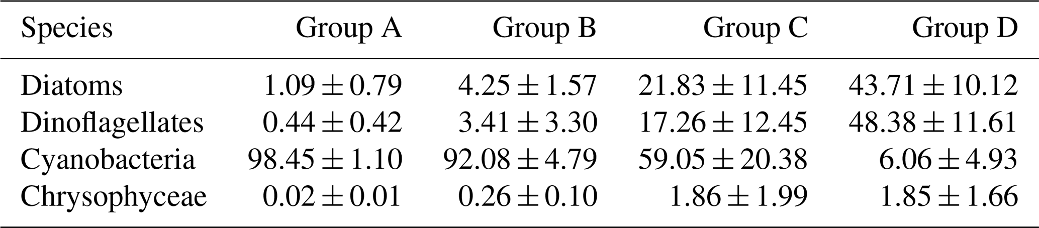
Since there was little interannual difference between species, we clustered all species based on Bray–Curtis similarity distance for stations, and the results showed four distinct regions (Fig. 6). Cluster analysis divided the phytoplankton communities at the sampling sites over 3 years into four groups. Cyanobacteria (>90 %) were the dominant species in Groups A and B. The species ratio of diatoms to dinoflagellates in Group A (dias: dinos = 4.8) was higher than that in Group B (dias: dinos = 1.4). Cyanobacteria were the dominant (66 %) phytoplankton at the stations of Group C, while diatoms (18 %) and dinoflagellates (14 %) constituted 32 % of the population in this group. Diatoms (43 %) and dinoflagellates (49 %) dominated the stations in Group D, accounting for approximately 92 % of the total phytoplankton. The proportion of Chrysophyceae was low in all four groups (Table 1). The dendrogram showed that these populations were grouped into four groups that were essentially identical to those determined by PCoA analysis (Fig. 7).

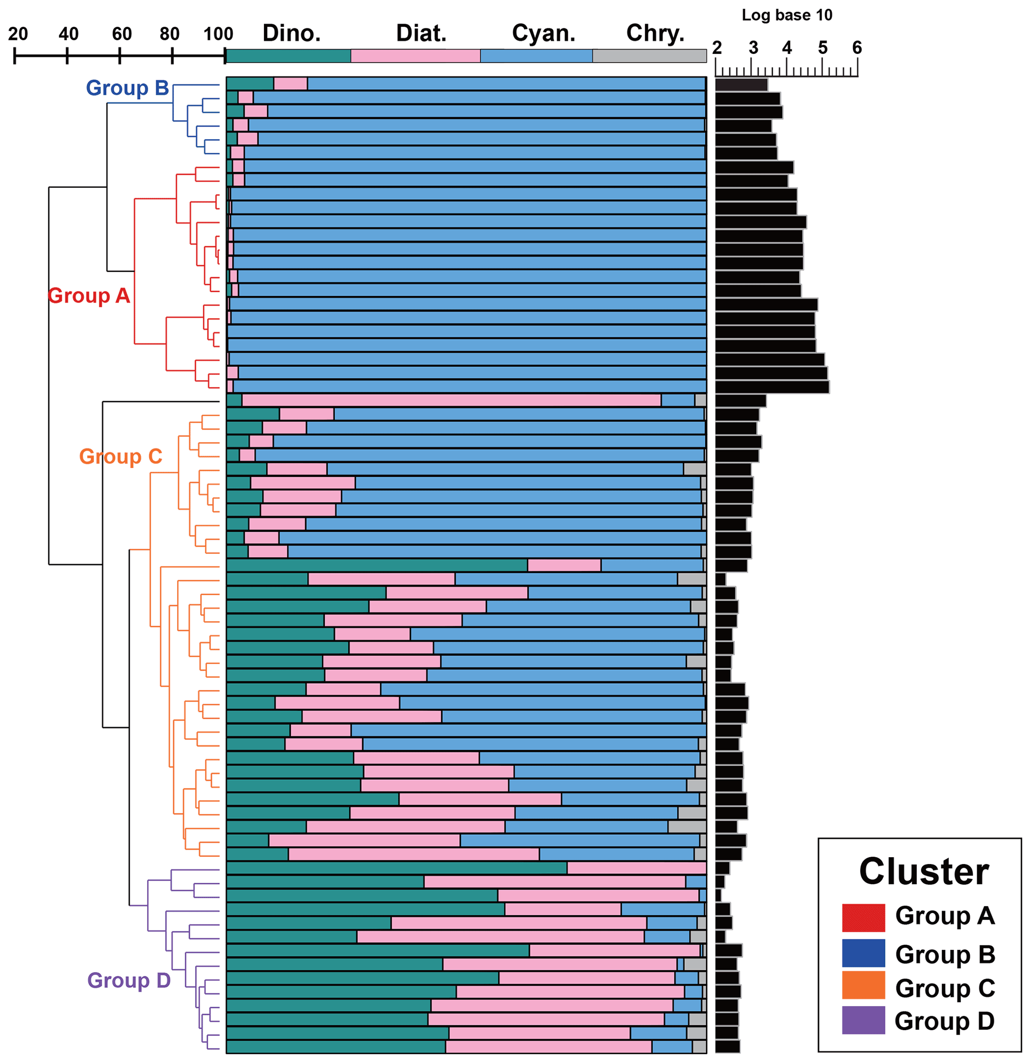
Figure 6 Bray–Curtis similarity-based dendrogram showing averaged phytoplankton community composition and abundance for each station across the three cruises. For each station, community composition is indicated with bar plots and phytoplankton abundance is represented with black bars.

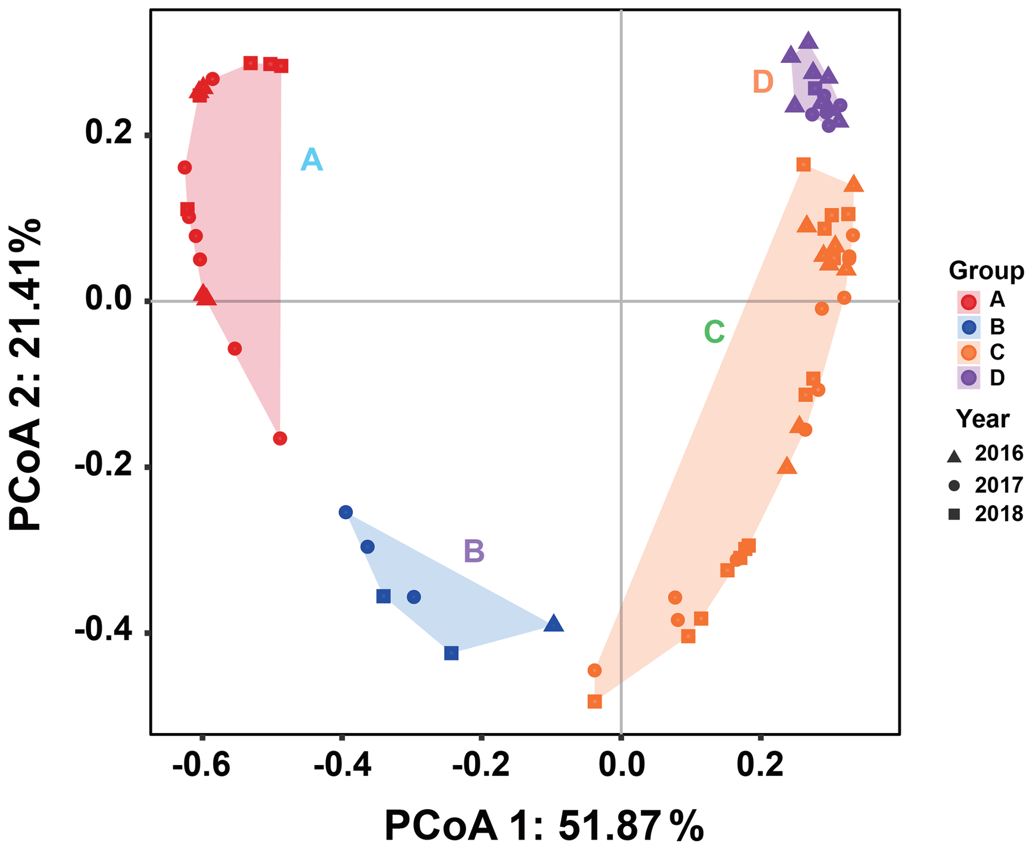
Figure 7 Principal coordinates analysis for groups. Triangles, circles, and squares represent 2016, 2017, and 2018 stations, respectively. P<0.05. Different colors represent different groups. Percentages of total variance are explained by coordinates 1 and 2, accounting for 51.87 % and 21.41 %, respectively.

Table 1 The percentages (%) (average ± standard deviation) of diatoms, dinoflagellates, cyanobacteria, and Chrysophyceae in the four groups.

3.5 Relationships between phytoplankton and environmental factors

The relationship between phytoplankton and environmental factors was analyzed using RDA. We obtained a two-dimensional distribution map of the species, sample distribution, and environmental factors (Fig. 8). The results showed that different phytoplankton classes were correlated differently with environmental factors. Cyanobacteria showed negative correlations with temperature and salinity and positive correlations with VSI and nutrient concentration, indicating that waters with high VSI are suitable for the growth of cyanobacteria (mostly Trichodesmium). Diatoms and dinoflagellates exhibited positive correlations with temperature and salinity and negative correlations with VSI and nutrient concentration, indicating that diatoms and dinoflagellates prefer waters with low VSI.

There were four distinct phytoplankton communities in the WPO: Group A was distributed in the equatorial region with clear vertical stratification. This community is characterized by high abundance and is dominated by Trichodesmium species such as T. thiebautii, T. hildebrandtii, and T. erythraeum, which are positively correlated with high concentrations of DIN, phosphate, and silicate. Group B was located near 8^∘ N and is mainly influenced by the NECC and mesoscale eddies; the phytoplankton community was represented by warm-water species, similar to that of Group A. Group C was mainly distributed in the 15^∘ N region and was strongly influenced by the NEC. Group D was mainly distributed in the 20^∘ N region, where it was directly influenced by the Kuroshio Current; here, the phytoplankton community was positively correlated with temperature and salinity.

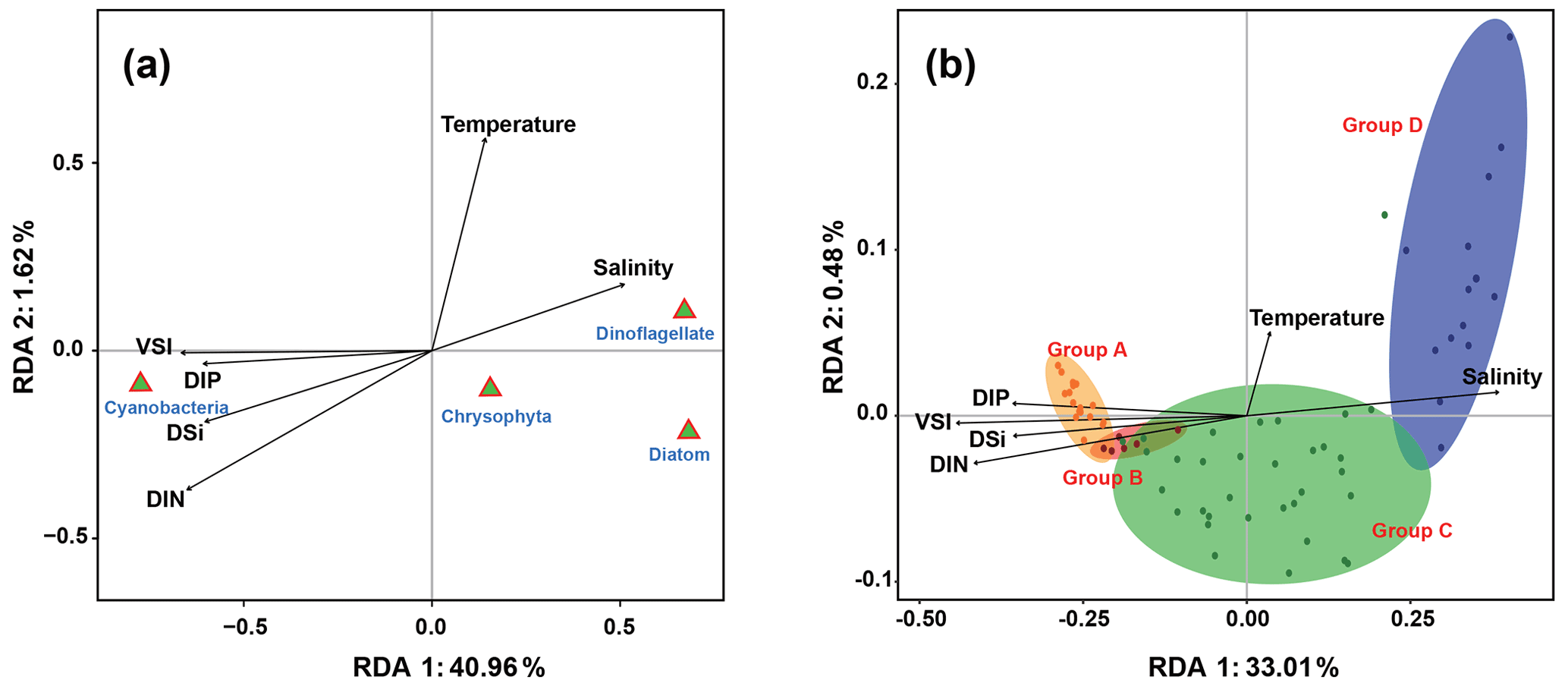
Figure 8 Redundancy analysis of the (a) phytoplankton and environmental parameters. (b) Groups and environmental parameters in the WPO. Colored dots represent sampling sites, triangles represent phytoplankton species, and arrows represent environmental factors.

3.6 Temperature, salinity, and vertical stratification index

The temperature, salinity, and VSI of the four groups are shown in Fig. 9. The temperature and salinity (T–S) box diagram depicts the four main water masses in the WPO. Groups A (average 29.8 ^∘C) and B (average 29.6 ^∘C) had high temperatures, but the salinities of Groups A (average 33.9 ^∘C) and B (average 33.8 ^∘C) were low. The temperature of Groups C (average 28.9 ^∘C) and D (average 28.9 ^∘C) were low, but the salinity of Groups C (average 34.2) and D (average 34.4) were high (Fig. 9a). Figure 9 shows clear variation in T–S, and we also calculated the vertical stratification index of the four groups (Fig. 9b). Compared with Groups C (average 3.86) and D (average 3.54), the values of VSI in Groups A (average 4.69) and B (average 4.86) were markedly higher, and Group A had the highest VSI. The stratification of the first two groups was more pronounced (Table 2).

The vertical stratification index was related to temperature (Fig. 9a) and salinity (Fig. 9b). Temperature is positively correlated with the vertical stratification index. The VSI of all groups was negatively correlated with salinity. The changes in temperature and salinity were most pronounced in the vertical direction. In Groups A and B with a high stratification index, the changes in temperature and salinity within the group were small. However, the temperature and salinity changed significantly within Groups C and D, with a small stratification index.

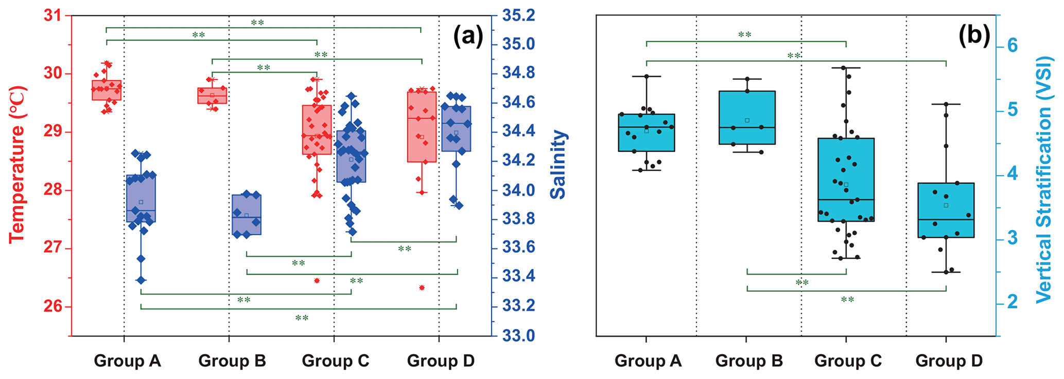
Figure 9 Surface temperature and salinity (a), and vertical stratification index (b) of the four groups.

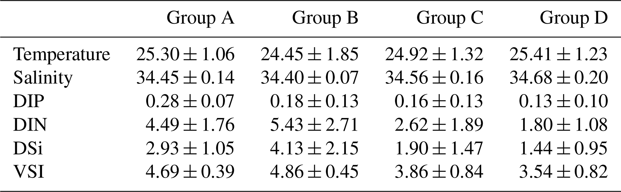
Table 2 Average (± standard deviation) values for nutrients (µmol L⁻¹), temperature (^∘C), and salinity for each phytoplankton community group identified by the cluster analysis in the WPO.

3.7 Direct vs. indirect effects of environmental parameters on phytoplankton abundance

The causal relationships between measured phytoplankton abundance and relevant physical and chemical parameters were examined using SEM, focusing on interactions between temperature, salinity, VSI, DIN, and DIP (Fig. 10) as theoretical and experimental data indicated the importance of these variables. The model results showed that temperature, DIP, and DIN had a direct effect on phytoplankton abundance, with temperature having the largest direct effect on phytoplankton abundance (0.38), followed by DIN (0.28) and DIP (0.24). Temperature, salinity, and VSI had indirect effects on phytoplankton abundance, with temperature and salinity having negative indirect effects on phytoplankton abundance (−0.17 and −0.30) and VSI having positive indirect effects (0.31) (Fig. 10). From the results of the total effect, only salinity had a negative effect on phytoplankton abundance (−0.30), while both temperature and VSI had positive effects on phytoplankton abundance (0.20 and 0.31), with VSI having the largest total effect. Although the direct effect of temperature on phytoplankton abundance was significant, it was partially offset by the indirect negative effect, while VSI had no direct effect on phytoplankton abundance, but its larger indirect effect resulted in the largest total effect. Both DIN and DIP had positive effects on phytoplankton abundance, but the effect of DIN was greater. Since the vertical distribution of DIN and DIP exhibited stronger variability, more specific analyses of DIN and DIP will be conducted later.

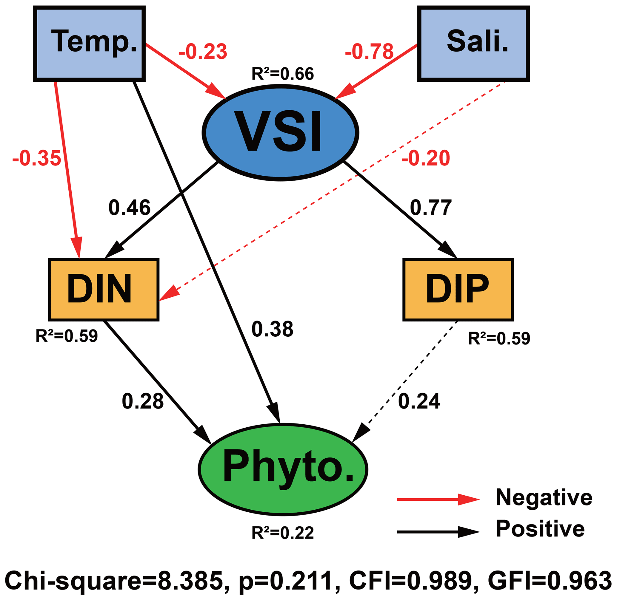
Figure 10 Structural equation model (SEM) analysis examining the effects of temperature, salinity, VSI, DIN, and DIP on phytoplankton abundance. Solid black and red lines indicate significant positive and negative effects at p<0.05, respectively, and dashed black and red lines indicate insignificant positive and negative effects, respectively. R² values associated with response variables indicate the proportion of variation explained by relationships with other variables. Values associated with arrows represent standardized path coefficients.

We analyzed the N : P ratio of the surface layer, the subsurface chlorophyll maximum (SCM) layer, and at 200 m. The N : P ratio in the surface layer (N : P > 16 : 1) indicates phosphorus limitation, which is consistent with the SEM analysis (Fig. 11). The trophic structure of the SCM layer changed, N : P < 16 : 1 indicated nitrogen limitation, and the depth continued to increase to the bottom of the euphotic layer and stabilized around N :P = 16 : 1, indicating that at the bottom of the euphotic layer, as phytoplankton abundance decreased and interspecific competition decreased, the trophic ratio approached the Redfield ratio and growth may have become increasingly limited by light.

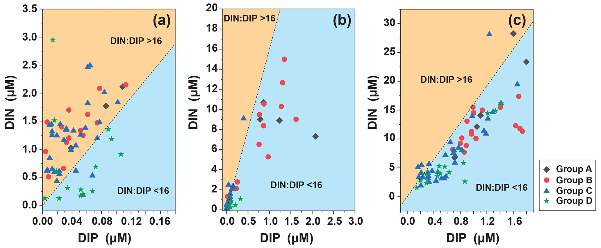
Figure 11 Distribution of phytoplankton community in DIN and DIP (a) at 5 m, (b) the SCM layer, and (b) at 200 m. The dashed line indicates the Redfield ratio of N : P = 16 : 1.

4 Discussion

4.1 Comparison with historical data

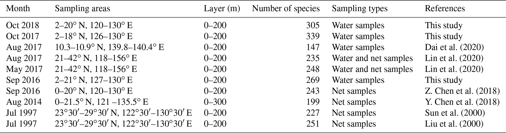
The Kuroshio Current and Western Pacific Warm Pool (WPWP) are key areas of the WPO sea–air interaction and climate modulation (Zhang, 1999). Previous surveys have provided less knowledge of the phytoplankton community structure in this study area (Table 3). Previously, samples were collected by net, and net-collected samples reduced phytoplankton abundance in small volumes, thereby underestimating the phytoplankton abundance in the ocean under investigation. In the present study, phytoplankton samples were collected from water samples, which better reflected the phytoplankton community structure and abundance. Sun et al. (2000) and Liu et al. (2000) further investigated the species composition and abundance distribution of phytoplankton diatoms and dinoflagellates in the Ryukyu Islands and nearby waters. Li et al. (2015) conducted a study on phytoplankton in the tropical and subtropical Pacific oceanic zones with response mechanisms to the limitation of nitrogen and iron. Y. Chen et al. (2018) investigated the phytoplankton community structure and mesoscale eddies in the western boundary current. A total of 199 species in 61 genera belonging to four phytoplankton families were identified, among which the abundance of Trichodesmium species was high. Previous studies have mostly focused on vertical hauls and the horizontal distribution of phytoplankton throughout the water column while ignoring the effect of vertical stratification on phytoplankton.

Table 3 Historical data of the phytoplankton community in the WPO.

4.2 Relationship between N : P ratio and vertical distribution of phytoplankton

Research into the factors that control the structure of the phytoplankton community has been carried out for decades, but the hypothesis of nutrient concentration limits and ratios has not been fully explained in terms of affecting the structure of the phytoplankton community (Gao et al., 2019). As diatoms and dinoflagellates show great differences in cell morphology, structure, and nutrition mode, they differ greatly in their nutrient acquisition strategies. Several studies have revealed that dinoflagellates use mixotrophy, engulfing prey and feeding using peduncles and pallia, while phosphorus limitation is a common factor stimulating dinoflagellates to ingest particulate nutrients (Huang et al., 2005; Smayda, 1997; Stoecker, 1999). The variation in phytoplankton community structure is always correlated with fluctuations in physicochemical environmental parameters.

In the four groups we studied, surface seawater N : P > 16 : 1 indicated that phosphorus in surface seawater was limited but that Trichodesmium relied on its own nitrogen fixation function and was highly abundant in oligotrophic waters (Fig. 6). The relationship between Trichodesmium and nitrogen fixation has already been demonstrated (Grosskopf et al., 2012; Luo et al., 2012; Zehr, 2011). The virtual absence nitrogen limitation in surface seawater in Group D was consistent with the low abundance of Trichodesmium, which was consistent with studies on the abundance of Trichodesmium in the region (Chen et al., 2019; Sohm et al., 2011). In the WPO, the most oligotrophic ocean in the world (Hansell and Feely, 2000), nutrients have become an important factor that determines the distribution of phytoplankton. Under nutrition-limited conditions, diatoms and dinoflagellates are more affected, especially under phosphorus limitation (Egge, 1998), which corresponds to the high abundance of Group D diatoms and dinoflagellates. In the present study, the vertical pattern of N : P ratios indicated differences in nutrient composition along the vertical gradient. The N : P ratio of the surface layer (N : P > 16 : 1) indicates phosphorus limitation. The structure of nutrients in the SCM layer changed, and (N : P < 16 : 1) indicates nitrogen limitation. The depth continued to increase to the bottom of the euphotic layer and was stable near (N : P = 16 : 1), indicating that at the bottom of the euphotic layer, where there is decreasing phytoplankton abundance, interspecific competition is reduced as light limitation kicks in, and the nutrient ratio approaches the Redfield ratio. The differences in nutrient ratios thus affect the vertical distribution patterns of phytoplankton abundance. Diatoms have higher phosphorus requirements than other phytoplankton groups, which may be reflected by the lower N : P ratio in diatoms than in other groups (Hillebrand et al., 2013). Iron is essential for the synthesis of nitrogen-fixing enzymes in Trichodesmium, and Trichodesmium has a higher demand for iron than other planktonic organisms. The main source of iron in the open ocean is atmospheric deposition. Duce and Tindale (1991) showed that the flux of iron deposition is higher in the WPO, and thus iron is an important environmental limiting factor for the growth of Trichodesmium in addition to temperature. We suggest that some of the sampled phytoplankton may have recently sunk from the upper layers and therefore represents nutrient rationing and T–S in the water layers. Directly sinking phytoplankton cells are major contributors to surface carbon export and an important component of ocean carbon sink (Boyd and Newton, 1999). The phytoplankton cells can regulate their sinking rates in a variety of ways, such as via their physiological state (Eppley et al., 1967), morphology (Pitcher et al., 1989), interaction with light (Bienfang, 1981), and interaction with environmental factors such as temperature and nutrients (Titman and Kilham, 1976).

4.3 Vertical stratification determined the vertical distribution of phytoplankton

The WPO is a oligotrophic area with strong stratification. We found that the interannual variation of phytoplankton was not significant. It remained stably oligotrophic, and the vertical stratification structure determined that of environmental resources such as nutrients, thus forming four contrasting environments, each with its characteristic phytoplankton community structure. Comparative analysis of the phytoplankton community composition of the four groups showed that the phytoplankton was mainly strongly affected by the vertical stratification, which corresponds to previous research (Bouman et al., 2011; Hidalgo et al., 2014; Mojica et al., 2015). Vertical stratification limits the replenishment of nutrients from the deep layer below the thermocline, which affects the N : P ratio and restricts vertical migration in addition to physiologically affecting the vertical structure of phytoplankton growth and mortality (Gupta et al., 2020).

In the present study, Trichodesmium was the dominant cyanobacterial species. Marine Trichodesmium is considered the most critical autotrophic nitrogen-fixing cyanobacteria (Dugdale et al., 1961). Trichodesmium can be divided into two forms: clusters and free filaments. Trichodesmium thrives in waters above 20 ^∘C and has a special cellular air sac structure that allows it to move vertically within the upper 100 m of the ocean water column (Laroche and Breitbarth, 2005). In the process of water blooms formed by Trichodesmium, a large amount of nitrogen is often fixed in a relatively short period of time. Therefore, the study of the nitrogen fixation rate of Trichodesmium is crucial for estimating the rate of nitrogen fixation in the ocean (Karl et al., 2002). Previous studies have not clarified which factors are the main causes of Trichodesmium growth (possibly temperature, wind, iron, phosphorus, etc.) (Capone et al., 1997; Chang et al., 2000; Sañudo-Wilhelmy et al., 2001; Karl and Tien, 1997). Many researchers have proposed that temperature is the most important factor affecting the growth of Trichodesmium (Capone and Carpente, 1999; Kustka et al., 2002). However, we suggest that there is no single positive correlation between temperature and Trichodesmium growth, which also is consistent with the study of Chang et al. (2000). In the tropical WPO, where the surface temperatures all exceeded 20 ^∘C, the abundance of Trichodesmium in areas with higher temperatures (Groups A and B) was higher than in those with lower temperatures (Groups C and D). Temperature not only directly affected phytoplankton growth but also indirectly affected phytoplankton growth and abundance by regulating VSI to drive the nutrient ratio (N : P) (Fig. 10).

Previous models and field experiments have shown that the species composition of phytoplankton communities is significantly affected by vertical turbulent mixing changes (Huisman et al., 2004). A strong coupling exists among the nutrient supply rate, the photosynthetic performance of phytoplankton (Bouman et al., 2006), and the phytoplankton biomass and primary production, particularly in eutrophic areas (Richardson and Bendtsen, 2019). The vertical stratification index reflects the potential effects of vertical stratification on various physical and chemical processes, such as regulating the utilization of light and nutrients in the ocean, which in turn affects phytoplankton dynamics. The results of the present study showed that from the Equator to the north, the VSI decreases as the latitude increases and that the phytoplankton community structure changes from cyanobacteria to diatoms. Phytoplankton abundance was significantly different in the water layer above the SCM. The water layer below the SCM tended to be stable. The surface phytoplankton abundance was usually greater than that of the SCM layer and was related to the surface layer of Trichodesmium. Our results demonstrate that the highly stratified region was more suitable for the growth of Trichodesmium, while the region with low vertical stratification seems to be more conducive to diatoms and dinoflagellates (Figs. 6 and 8). Due to their low mobility and high potential growth rate, diatoms can reproduce rapidly in mixed water with high nutrient content (Tilman et al., 1986). The weak vertical stratification of the Group C and D regions (Fig. 9b) leads to relative homogeneity of temperature, salinity, density, and nutrients in the upper layer of 200 m in the vertical direction (Pérez et al., 2006). The vertical distribution of zooplankton has shown that vertical stratification can hinder the migration of small zooplankton populations and indicate different grazing pressures (Mitra and Flynn, 2005; Long et al., 2021). Further research should consider the difference in predation pressure of different zooplankton predators on the composition of the phytoplankton community in different regions. Phytoplankton stratification may cause thin-layer algal blooms and other phenomena, and the influence of phytoplankton stratification can be investigated in further studies.

5 Conclusions

This study investigated the phytoplankton community structure of the WPO in the autumn of 2016, 2017, and 2018. The WPO is a oligotrophic ocean with a weak water exchange capacity owing to the thermocline and severe stratification in the upper seawater layer. The phytoplankton community structure mainly consisted of cyanobacteria, diatoms, and dinoflagellates, while the abundance of Chrysophyceae was low. In terms of spatial distribution, phytoplankton abundance was high from the equatorial region to 10^∘ N and decreased with increasing latitude. Phytoplankton showed a high variation in the vertical distribution. The potential influences of physicochemical parameters on phytoplankton abundance were analyzed by a structural equation model (SEM) to determine nutrient ratios driven by vertical stratification to regulate phytoplankton community structure in a typical oligotrophic sea area. Regions with strong vertical stratification (Groups A and B) were more favorable for cyanobacteria, whereas weak vertical stratification (Groups C and D) was more conducive to diatoms and dinoflagellates.