the Creative Commons Attribution 4.0 License.
the Creative Commons Attribution 4.0 License.
 | 26 Oct 2021
Decadal sea-level variability in the Australasian Mediterranean Sea
Claus W. Böning
Strong regional sea-level trends, mainly related to basin-wide wind stress anomalies, have been observed in the western tropical Pacific over the last 3 decades. Analyses of regional sea level in the densely populated regions of the neighbouring Australasian Mediterranean Sea (AMS; also called tropical Asian seas) are hindered by its complex topography and respective studies are sparse. We used a series of global eddy-permitting ocean models, including a high-resolution configuration that resolves the AMS with ∘ horizontal resolution, forced by a comprehensive atmospheric forcing product over 1958–2016 to characterize the patterns and magnitude of decadal sea-level variability in the AMS. The nature of this variability is elucidated further by sensitivity experiments with interannual variability restricted to either the momentum or buoyancy fluxes, building on an experiment employing a repeated-year forcing without interannual variability in all forcing components. Our results suggest that decadal fluctuations of the El Niño–Southern Oscillation (ENSO) account for over 80 % of the variability in all deep basins of the region, except for the central South China Sea (SCS). Changes related to the Pacific Decadal Oscillation (PDO) are most pronounced in the shallow Arafura and Timor seas and in the central SCS. On average, buoyancy fluxes account for less than 10 % of decadal SSH variability, but this ratio is highly variable over time and can reach values of up to 50 %. In particular, our results suggest that buoyancy flux forcing amplifies the dominant wind-stress-driven anomalies related to ENSO cycles. Intrinsic variability is mostly negligible except in the SCS, where it accounts for 25 % of the total decadal SSH variability.
- Article
(3628 KB) - Full-text XML
- BibTeX
- EndNote


Between the early 1990s and mid-2010s sea-level trends of up to 10 mm yr−1, which exceeds 3 times the global mean rate, were observed in the western tropical Pacific and found to be related to an intensification of the Pacific trade wind regime (Timmermann et al., 2010; Merrifield, 2011; Merrifield and Maltrud, 2011; McGregor et al., 2012; Merrifield et al., 2012; Moon and Song, 2013; Moon et al., 2013; Qiu and Chen, 2012). This strong sea-level rise had severe consequences for the population of the low-lying islands in the region (Becker et al., 2012), whose inhabitants are regularly referred to as the first climate refugees. Sea-level changes in the western tropical Pacific received a lot of scientific attention. Despite the exposed position of many densely populated coastal communities, this is not true for the neighbouring areas of the Australasian Mediterranean Sea (AMS; see Fig. 1 for an overview map of the study domain). For the period 1993–2009 strong trends of up to 9 mm yr−1 were observed in the southwestern part of the region, but trends are not uniform across the many small seas of the region (Strassburg et al., 2015) and studies on regional sea-level variability in the region are sparse.
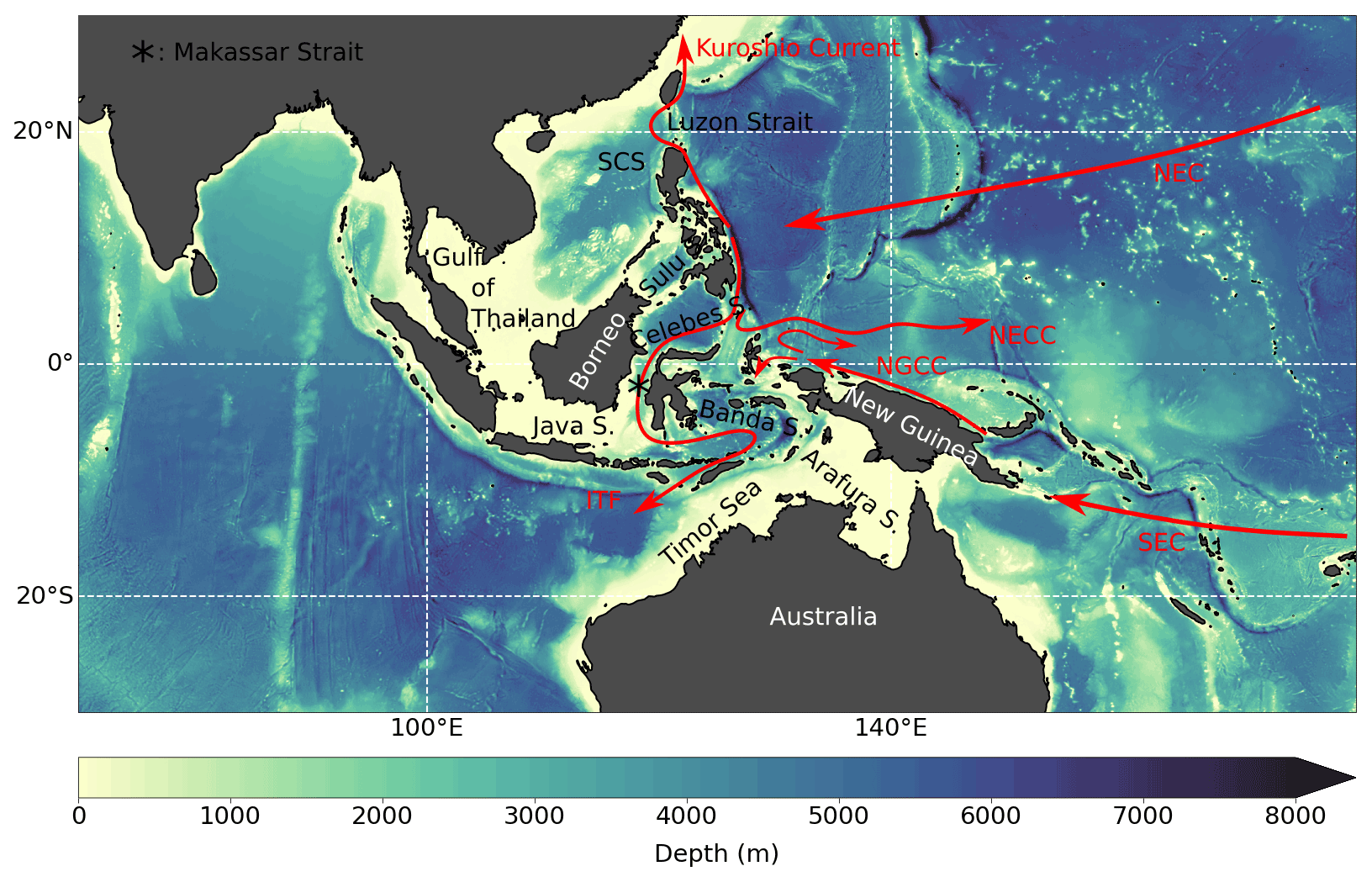
Figure 1Overview map of study domain, depicting the marginal seas and schematic currents discussed in the text. Colour shading indicates depth. Marginal seas, islands, continents, and schematic currents that are mentioned in the text are also marked. SCS: South China Sea, NEC: North Equatorial Current, SEC: South Equatorial Current, NECC: North Equatorial Countercurrent.
The best studied area in the region in terms of sea level is the South China Sea (SCS). It is the largest marginal sea of the region. The central and northeastern deep parts of the basin show the largest amplitudes of interannual and decadal variability (Cheng and Qi, 2007), with trends of up to 8 mm yr−1 for the period 1993–2012 (Cheng et al., 2016). There is a broad consensus that the El Niño–Southern Oscillation (ENSO) has a strong impact on interannual sea-level variability (Cheng and Qi, 2007; Cheng et al., 2016; Rong et al., 2007; Wu and Chang, 2005; Fang et al., 2006; Peng et al., 2013). Subsurface heat content anomalies are advected into the basin via the Luzon Strait (Cheng and Qi, 2007; Rong et al., 2007), and coastal Kelvin waves advect anomalies related to ENSO and possibly the Pacific Decadal Oscillation (PDO) from the tropical Pacific clockwise around the Philippines into the SCS (Liu et al., 2011; Zhuang et al., 2013; Cheng et al., 2016). Local wind stress curl, also related to ENSO, might amplify these sea-level anomalies in the central SCS (Cheng et al., 2016). In contrast, Kleinherenbrink et al. (2017) did not find a strong impact of tropical wind stress variability on sea-level changes in the SCS.
Sea-level variability in the southeastern part of the AMS, i.e. between Borneo and Australia, has received much less attention. However, the area has been of great interest since it represents the only low-latitude connection of ocean basins (Sprintall et al., 2014) and acts as an upper pathway of the global overturning circulation (Gordon, 1986). The main circulation feature is the Indonesian Throughflow (ITF) that transports heat and fresh water from the Pacific into the Indian Ocean (Gordon, 2005). The ITF variability on interannual timescales is mostly a response to variations of the Pacific trade winds governed by large-scale climate modes. In particular, ENSO has a strong effect on ITF transport on interannual timescales (Meyers, 1996; Wijffels and Meyers, 2004; Liu et al., 2015). Decadal ITF variability is also linked to shifts of the Pacific trade wind regime (Wainwright et al., 2008; Liu et al., 2010; Zhuang et al., 2013; Feng et al., 2011, 2015), but other mechanisms, like deep Pacific upwelling (Feng et al., 2017), could also play a role. However, given the impact of Pacific easterlies on ITF variability, it is reasonable to assume that sea level along the ITF pathways is also remotely controlled by the Pacific trade wind regime. Indeed, sea-level variability along the Australian west coast is closely linked to variability in the western tropical Pacific (Feng et al., 2004; Lee and McPhaden, 2008; Merrifield et al., 2012). This requires a way for signals to cross the AMS. The theory of an equatorial waveguide that allows remote forcing of variability in the throughflow region was already proposed in 1994 (Clarke and Liu, 1994). Wijffels and Meyers (2004) showed, based on XBT (expendable bathythermograph) observations from 1984 to 2001, that sea-level anomalies propagate from the Pacific Ocean along the Papuan and Australian shelf break into the Indian Ocean and that interannual variability is driven by remote wind forcing from the Pacific.
In a more detailed analysis, Kleinherenbrink et al. (2017) separated observed sea-level changes between 2005 and 2012 into mass and steric components. They found mass changes to be relevant in the shelf regions, where a shallow water column is unable to expand due to density changes. Furthermore, they reported that the deep basins of the Banda and Celebes seas show large steric sea-level variability on interannual timescales, which appear to be linked to wind stress anomalies over the tropical Pacific. Using the Dipole Mode Index (DMI; Saji et al., 1999) they also found an impact of the Indian Ocean that is, however, limited to the Timor Sea. Strassburg et al. (2015) could also link observed and reconstructed decadal sea-level trends between 1950 and 2009 to PDO-related wind stress changes over the tropical Pacific.
Comparatively little is known about the importance of local or remote buoyancy fluxes that have been proven to be relevant for sea level in other parts of the world's ocean, including the tropical Pacific (e.g. Piecuch and Ponte, 2011; Piecuch et al., 2019; Wagner et al., 2021). Cheng and Qi (2007) suggested an influence of ocean–atmosphere freshwater fluxes on halosteric sea level in the SCS. In particular, the observed decrease between 2001 and 2005 was found to coincide with a salinification trend due to reduced freshwater fluxes. Rong et al. (2007) pointed out that local precipitation anomalies are the primary control of the SCS mass budget and thereby also influence sea level.
Using ocean and climate models to analyse sea level in this region is hindered by its complex topography that forms many small seas and narrow straits. For example, the Labani channel, the deep part of the Makassar Strait and the main pathway of the ITF, is only about 40 km wide, which is barely resolved in an ∘ ocean model, let alone in even coarser climate models. We therefore used a series of ocean model experiments that consists of two hindcast simulations subject to realistic atmospheric forcing covering the last 6 decades and providing horizontal resolution of and ∘, supplemented by a series of sensitivity experiments that allow an individual application of momentum and buoyancy flux forcing to the underlying ocean. The aim of this study is to examine the sea-level variability in the AMS in high-resolution ocean model simulations subject to atmospheric forcing over the last 6 decades. In particular, the objectives are the following:
-
to elucidate the patterns and nature of the regional sea-level variability on decadal to multi-decadal timescales, including the impacts of the low-frequency ENSO and PDO changes which have been identified in previous studies as major drivers of sea-level variability on interannual to decadal timescales;
-
to examine the possible contribution of intrinsic variability, internally generated by ocean dynamics, to the total sea-level variability in the region and to determine the relative roles of momentum and buoyancy fluxes in the forced variability; and
-
to analyse the individual contributions of temperature and salinity changes to steric sea-level variability.
Concerning the notation of the marginal seas between Australia and Asia, some deviating conventions have been used in the natural science community since international standards have not been officially updated since 1953 (International Hydrographic Organisation, 1953). Examples are “tropical Asian seas” (Kleinherenbrink et al., 2017), “southeastern Asian seas” (Strassburg et al., 2015), and “Australasian Mediterranean Sea” (AMS; Tomczak and Godfrey, 2003). We adapted the latter for the purpose of this study and refer to all marginal seas in the region, including the Timor and Arafura seas and also the SCS, as AMS. It will be useful to point to the SCS and the remaining part of the region individually. We use the term “Eastern Archipelagic Seas” (EAS) for this purpose.
2.1 Ocean general circulation model experiments
We used a global ocean model configuration of the Nucleus for European Modelling of the Ocean (NEMO) code version 3.6 (Madec and NEMO-team, 2016). The model employs a global tripolar ORCA grid and uses 46 vertical z levels with varying layer thickness from 6 m at the surface to 250 m in the deepest levels. Bottom topography is represented by partial steps (Barnier et al., 2006) and is interpolated from 2 and 1 min Gridded Global Relief Data ETOPO2v2 (http://www.ngdc.noaa.gov/mgg/global/relief/ETOPO2/ETOPO2v2-2006/ETOPO2v2g/, last access: 12 June 2018) and ETOPO1 (https://www.ncei.noaa.gov/access/metadata/landing-page/bin/iso?id=gov.noaa.ngdc.mgg.dem:316, last access: 11 October 2019, Amante and Eakins, 2009) for the coarse- and high-resolution experiments, respectively. The atmospheric forcing for all experiments is JRA55-do v1.3 (Tsujino et al., 2018), which builds on the JRA-55 reanalysis product but is specifically designed to be used as a forcing dataset for ocean general circulation models (OGCMs). Most importantly, surface fields are corrected towards observations, and heat and freshwater fluxes are balanced with respect to a defined set of bulk formulas. Laplacian and bi-Laplacian operators were used to parameterize horizontal diffusion of tracers and momentum, respectively. The ocean model was coupled to the Louvain-La-Neuve sea-ice model version 2 (LIM2-VP; Fichefet and Maqueda, 1997). To avoid spurious drifts of global freshwater content, all models used a sea surface salinity restoring with piston velocities between 137 and 40 mm d−1. The coarse-resolution experiments additionally used a freshwater budget correction that sets changes in the global budget to zero at each model time step.
In order to increase the horizontal resolution in the area of interest, a high-resolution “nest” was incorporated into the global base model. This approach allows a regional refinement of the horizontal resolution to ∘ in the area from 50∘ S to 25∘ N and 75 to 180∘ E. The nesting technique is based on adaptive grid refinement in Fortran (AGRIF; Debreu et al., 2008). A two-way communication was established between the high-resolution nest and the global “coarse-resolution” model. The base model provided boundary conditions for the nest at every time step of the nest (the base model and the nest were integrated with a time step of 5 and 15 min, respectively). Due to the higher resolution of the nest in time and space, the boundary conditions were interpolated. The prognostic variables along the boundary of the nest were in turn updated after every time step of the base model by the calculations provided by the nest. Every three time steps, the full baroclinic state vector of the nest was averaged onto the base grid and fed back to the base model. This approach is well established, and the reader is referred, for example, to Schwarzkopf et al. (2019) for a detailed description of the procedure.
We integrated two reference configurations with interannually varying atmospheric forcing from 1958 to 2016.
-
REF005. This is a reference run with ∘ horizontal resolution globally and ∘ in the nest area.
-
REF025. This is a reference run with ∘ horizontal resolution globally.
In addition, we followed the approach of Stewart et al. (2020) to construct a “quasi-climatological” forcing. More specifically, we extracted the recommended 12-month subset from May 1990 to April 1991 from the full forcing dataset and applied its individual fields repeatedly to suppress the interannual variability entirely or only for the computation of momentum or buoyancy fluxes, respectively. This way, we obtained three additional sensitivity experiments with ∘ horizontal resolution globally, which were all integrated for 59 years to match the length of the reference configurations.
-
CLIM: full quasi-climatological forcing
-
WIND: quasi-climatological buoyancy fluxes
-
BUOY: quasi-climatological momentum fluxes
The experiments WIND and BUOY are meant to isolate the momentum-flux-forced and buoyancy-flux-forced variability. The approach builds on the assumption that the total atmospherically forced variability can approximately be understood by a linear combination of these two contributions. Because we only suppress variability on interannual and longer timescales, this assumption is not valid for variability on shorter timescales. A possible deviation could also arise from non-linearities and intrinsic, i.e. unforced, variability: an estimate of the magnitude of the latter is provided by the experiment CLIM. We note that the set of ∘ experiments (REF025, WIND, BUOY, and CLIM) has been used previously for studies of Indian Ocean heat content (Ummenhofer et al., 2020), marine heatwaves (Ryan et al., 2021), and tropical Pacific sea-level variability (Wagner et al., 2021).
2.2 Observational datasets
We used two observational datasets to validate our model results. Satellite altimetry data are provided as a gridded product by the Copernicus Marine Environment Monitoring Service (https://resources.marine.copernicus.eu/?option=com_csw&view=details&product_id=SEALEVEL_GLO_PHY_L4_REP_OBSERVATIONS_008_047, last access: 12 June 2018) (CMEMS) with a resolution of ∘ that is available starting in 1993 (in contrast to our model simulations that start in 1958). Observations of temperature and salinity were taken from the World Ocean Atlas 18 (https://www.ncei.noaa.gov/archive/accession/NCEI-WOA18, last access: 16 February 2021) (WOA18; Locarnini et al., 2019; Zweng et al., 2019) that is also available with ∘ horizontal resolution and covers the period from 1958 to 2017.
2.3 Steric sea level
Sea-level changes are either due to changes in the total mass of the water column or due to density changes in seawater. The latter is referred to as steric sea level. Because seawater density is affected by temperature and salinity, steric sea level and can be separated into thermosteric and halosteric components, respectively. We diagnosed steric sea-level changes from the stored model output:
where (η) denotes sea level, ρ is seawater density, and H is ocean depth. Thermosteric sea-level changes are given by
where α is the thermal expansion coefficient and Θ is potential temperature. In the same way, halosteric sea-level variations can be expressed as
where β is the haline contraction coefficient and S is salinity.
First, we compare our model results to observational products for validation and to point out some resolution-dependent biases. Sea-level observations from satellite altimetry show strong interannual sea surface height1 (SSH) variability in the western tropical Pacific off the east coast of the Philippines islands. Within the AMS, variability is most pronounced in the deep basins of the SCS and the adjacent Sulu, Celebes, and Banda seas as well as in the coastal regions of the Arafura and Timor seas (Fig. 1). Both hindcast simulations slightly underestimate the amplitude of standard deviation (SD), in particular in the western tropical Pacific, by 1 to 2 cm (REF025 and REF005, respectively) but reproduce the spatial pattern well (Fig. 2b, c). The spatial average of SSH over the AMS (see black contour in Fig. 2c) reveals interannual to decadal variability. The latter is more pronounced in the high-resolution configuration (REF005) and agrees well with the observed positive trends since the early 90s (Fig. 2d).
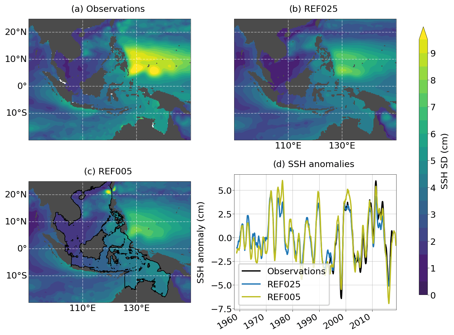
Figure 2SD of SSH from (a) observations and two hindcast experiments, (b) REF025 and (c) REF005, over the period 1993 to 2016. (d) SSH anomalies averaged over the region marked by black contours in panel (c). The global mean trends over the integration period have been subtracted, and all data were smoothed with a 12-month running mean window.
Figure 3 shows subsurface maps of mean fields and model biases of temperature and salinity with respect to observations from WOA18, averaged over the upper 400 m, from both hindcast simulations. Both hindcasts exhibit some temperature biases, in particular in the tropical Pacific, where opposite signs right on the Equator and at about 8∘ N (Fig. 3a–c) indicate a large-scale southward displacement of the Intertropical Convergence Zone (ITCZ) in the Pacific that causes a southward shift of the equatorial upwelling regime. The coarse-resolution hindcast REF025 also shows positive temperature and salinity biases in the AMS, in particular in the northern part of the SCS, where values exceed 3∘ and 0.3 psu (Fig. 3b, e). These biases are greatly reduced in the high-resolution setup to temperature biases well below 0.5 ∘C and salinity biases below 0.1 psu.
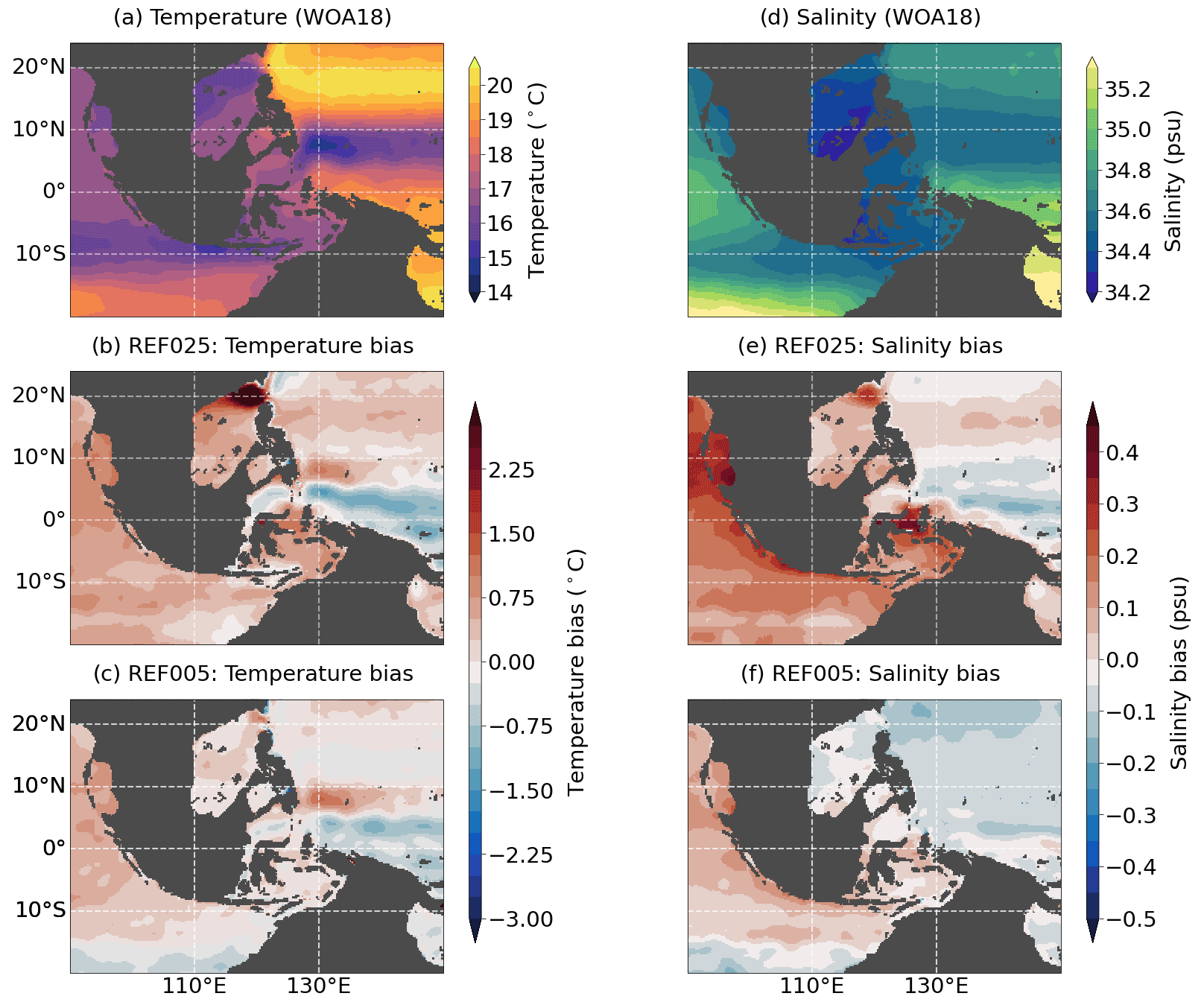
Figure 3Mean fields (1955–2017; a, b) and model biases (1958–2016; b, e, c, f) averaged over the upper 400 m for (a–c) temperature and (d–f) salinity. Note that data are only shown where the water depth exceeds 400 m.
3.1 Impact of buoyancy fluxes on SSH
We now turn to the forcing mechanism of decadal SSH variability and inspect the low-pass-filtered (cutoff period of 8 years) SSH time series. Figure 4 presents maps of standard deviation (SD) for all five experiments, as well as SSH anomalies averaged over the AMS. The two hindcast simulations show a close resemblance in terms of amplitude and pattern, suggesting only a minor influence of the model resolution (Fig. 4a, b). The pattern and amplitude of the WIND experiment (Fig. 4c) closely match the signal in REF025, indicating that wind stress variability is the most important driver of the variability. The SSH signal driven by the interannual variability of buoyancy fluxes shows much lower amplitudes and a different spatial pattern (Fig. 4d; note the different colour bars): it is most pronounced outside the AMS in the Kuroshio region and the southeastern tropical Indian Ocean and within the AMS in the SCS, whereas values in the EAS are relatively low (about 0.3–0.4 cm).
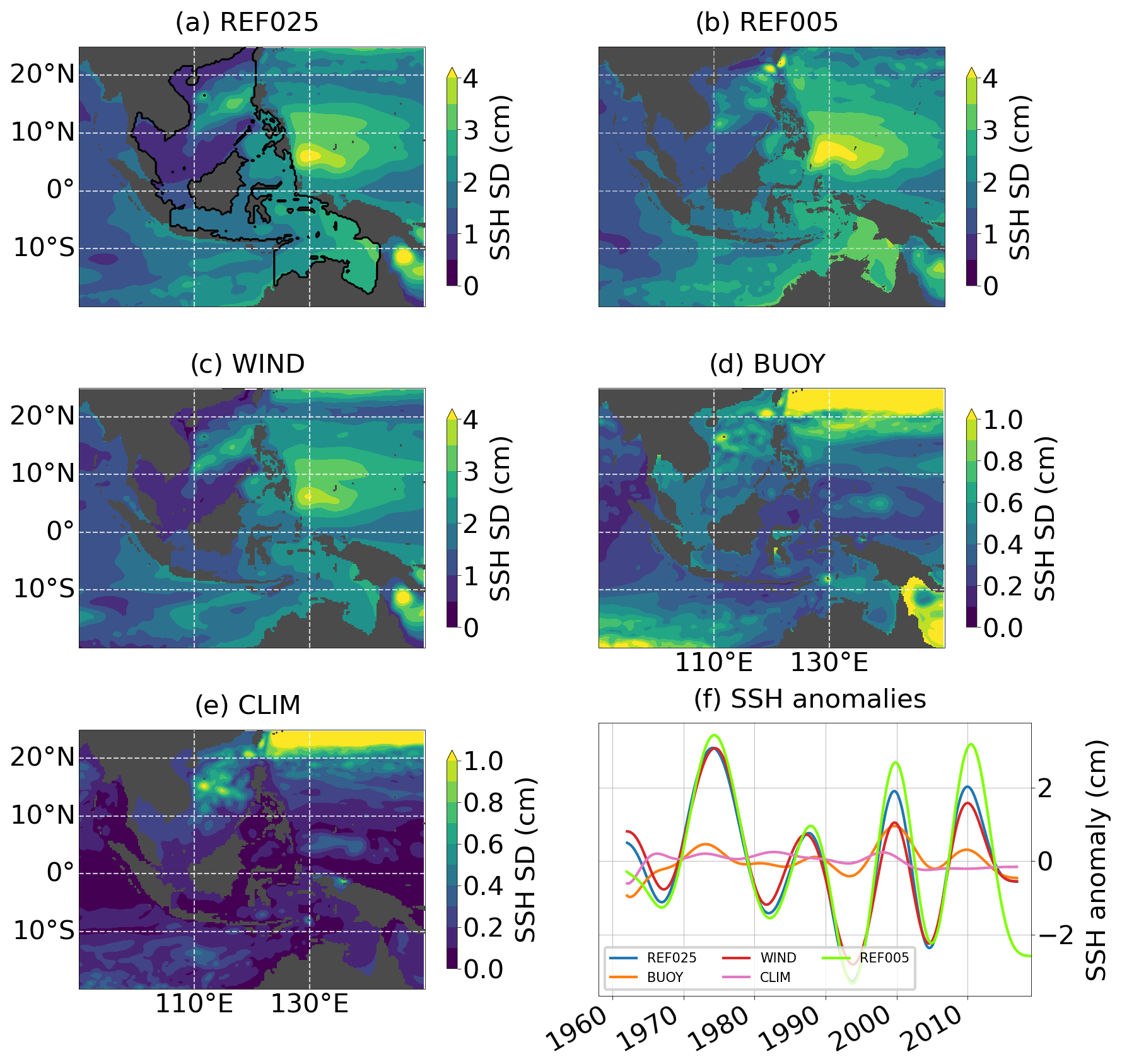
Figure 4SD of low-pass-filtered SSH time series (8 years) from (a) REF025, (b) REF005, (c) WIND, (d) BUOY, and (e) CLIM as well as (f) low-pass-filtered SSH anomalies averaged over black contour lines shown in panel (a). Note the different colour bars.
While in most areas the total variability in REF025 can be understood as a linear superposition of variability due to momentum and buoyancy fluxes, this is not the case in the Kuroshio region or the Gulf of Thailand. Possible reasons are cancelling effects of out-of-phase variations of momentum and buoyancy fluxes or, as pointed out above, intrinsic ocean variability and non-linear effects. As evident from Fig. 4e, intrinsic variability in the AMS is below 0.2 cm everywhere except in the SCS. Amplitudes in the northern SCS reach values of up to 1 cm and are thereby comparable to the values of the buoyancy forcing experiment and account for about 25 % of the total variability in REF025.
Averaged over the AMS, buoyancy fluxes amplify the wind-stress-driven variability (Fig. 4f). If we consider the change in variability between REF025 and WIND, rather than the variability in BUOY itself, to be the effect of buoyancy fluxes, we find a contribution of 9 % (SD of 1.54 cm in REF025 and 1.4 cm in WIND) by which buoyancy fluxes amplify the wind-stress-driven variability. This fraction is, however, variable over time and reaches values of up to 50 %, for example, during the late 1990s. When estimating the effect of buoyancy fluxes from BUOY directly, we obtain a much larger contribution of 24 %. The reason for this is intrinsic variability that is included in all experiments and adds to the variability in BUOY. We found no indication that buoyancy fluxes contribute to the increase in sea level between roughly 1990 and 2010 that is visible in both hindcast simulation and WIND.
3.2 Linear regression of SSH on ENSO and PDO indices
A linear regression model is used to quantify the impact of low-frequency ENSO changes and PDO cycles on sea-level variability. We use a bandpass-filtered Niño3.4 index2 (8–13 years) and a low-pass-filtered PDO3 index (13 years) as predictors. Both indices are derived from REF025 and compare well with observational estimates (Fig. A1). Both indices are not significantly correlated (at a confidence interval of 5 %) by construction because their variability is limited to timescales longer or shorter than 13 years. This allows a linear superposition of the responses and their respective coefficients of determination (R2 gives the fraction of variance explained by a linear model; e.g. Thomson and Emery, 2014). As before, SSH data have been low-pass-filtered (8 years) prior to the regression. Note that the PDO can be considered the low-frequency component of ENSO in this context to the extent that the PDO can be regarded as the low-frequency component of ENSO; an alternative and largely equivalent separation could be built on the low-pass-filtered Niño3.4 index instead of the PDO index. We will get back to this point in Sect. 4. The Indian Ocean Dipole Index (IOD; Saji et al., 1999) could account for possible impacts of the Indian Ocean. We do not include the IOD in our analysis because the index shows only very weak variability on the timescales considered here (not shown).
Figure 5 depicts the linear responses of SSH from three experiments to the Niño3.4 and PDO indices. Since its results are very similar to REF025, we omit the WIND case here but refer to it in the Appendix (Fig. A2). REF025 and REF005 show a similar response to positive ENSO cycles (Fig. 5a, b). Strong negative anomalies in the western tropical Pacific with amplitudes of 4 cm off the east coast of the Philippines islands leak into the northeastern part of the SCS and also follow the equatorial waveguide across the Celebes and Banda seas as well as along the Australian shelf break into the Indian Ocean. Here, both hindcasts find amplitudes between 1 and 2 cm (Fig. 5 a, b). This pattern is mostly determined by wind stress variability, as the wind stress experiment shows similar results (Fig. A2) and the pattern in BUOY differs strongly (Fig. 5c). Here, SSH shows a weak but non-negligible negative response to ENSO cycles which is uniform across the domain and thereby amplifies the wind-stress-driven response by about 0.2–0.3 cm in most parts of the region. Buoyancy fluxes counteract the wind-stress-driven variability off the northeastern coast of Australia, to the south of Papua New Guinea, such that the effective ENSO-related SSH variability is almost zero.
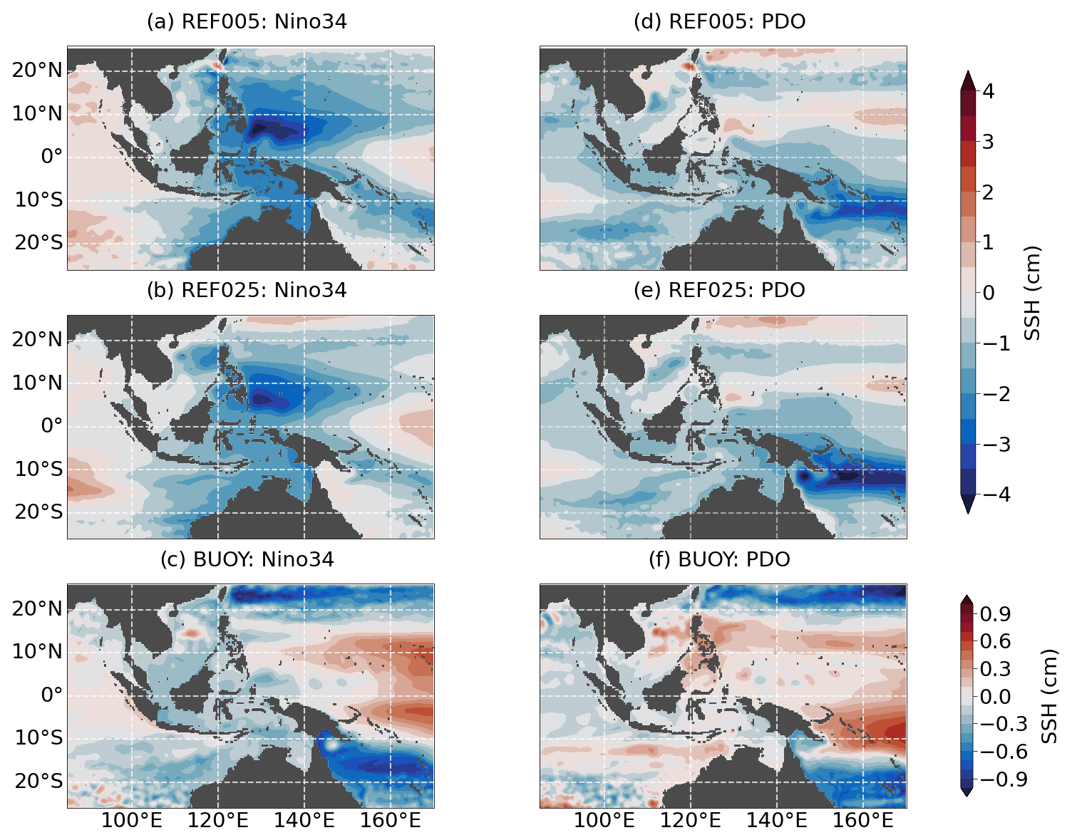
Figure 5Linear regression of SSH with the (a–c) Niño3.4 index and (d–f) PDO index for two hindcast (REF025, REF005) and buoyancy forcing experiments (BUOY). Climate indices are derived from the base model in the case of REF005 and from REF025 for the other two experiments. All data have been filtered with an 8-year low-pass filter. Note the different colour bars.
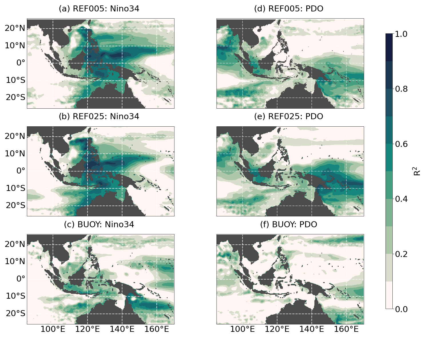
Figure 6Coefficient of determination for the linear regression of SSH with the (a–c) Niño3.4 index and (d–f) PDO index for two hindcast (REF025, REF005) and buoyancy forcing experiments (BUOY). Climate indices are derived from the base model in the case of REF005 and from REF025 for the other two experiments. All data have been filtered with an 8-year low-pass filter.
The linear response to the PDO index shows strong amplitudes of 3 and 4 cm (in REF005 and REF025, respectively; Fig. 5d, e) to the east of Papua New Guinea in the region of the South Pacific Convergence Zone (SPCZ). Anomalies stretch northwestward along the shelf and into the EAS, in particular into the Arafura seas, with values between 1 and 2 cm. Both hindcast experiments also suggest a PDO imprint in the Java seas and the central SCS. Again, the variability is mostly driven by momentum fluxes (Fig. A2). Buoyancy fluxes cannot explain the dominant pattern and tend to dampen the variability regionally, in particular in the SPCZ, but also in the western tropical Pacific north of 10∘ N, in the northern part of the SCS, and in the Sulu Sea. The response in the remaining regions is mostly below 0.1 cm.
In order to determine what fraction of the total variability can be explained by these two climate indices, Fig. 6 displays R2. Both hindcasts (and also the WIND experiment; Fig. A2a) agree that ENSO determines a large fraction of the low-frequency variability in the western tropical Pacific at around 5∘ N, in all deep basins with values of over 80 %, and, to a slightly lesser extent, also in the Timor Sea and along the Australian shelf break. This fraction is reduced to less than 50 % for the buoyancy-flux-related variability (Fig. 6c).
Both hindcast simulations find that over 50 % of the total decadal SSH variability in the SPCZ and the Java Sea and over 30 % in the central SCS can be explained by PDO cycles. Both differ in their estimate of the quantitative importance of the PDO for the remaining region of the EAS, but still find 10 %–20 % of explained variance in the case of REF005 and even more in REF025. Note, however, that REF025 showed temperature and salinity biases in this region that might be the reasons for these discrepancies. The PDO does not drive any buoyancy-flux-driven SSH variability in the AMS (Fig. 6f). The linear combination of the two indices (not shown) gives high scores of over 80 % throughout the domain except in the central and southern part of the SCS where intrinsic variability is relevant.
3.3 Decomposition of SSH variability into thermosteric and halosteric contributions
To further elucidate the mechanisms shaping the sea-level signal, it is useful to analyse the dynamical response and also decompose the sea-level signal into its steric components. We neglect sea-level anomalies due to mass fluctuations because their relative contributions are small everywhere except on shelf regions (not shown; e.g. Forget and Ponte, 2015) where the total variability is weakest.
As expected, the dynamical response to the ENSO cycles (Fig. 7a–c) is governed by anomalies of the North Equatorial Countercurrent at 4∘ N and by thermosteric SSH anomalies of over 4 cm in the western tropical Pacific. The latter change the inter-basin pressure gradient between the Pacific and the Indian Ocean. Specifically, a positive ENSO cycle leads to a reduction in SSH, which causes a decreased pressure gradient across the AMS. Consequently, northward velocity anomalies in the Makassar Strait and Banda Sea indicate a reduction of ITF transport. Steric changes are consistent with this dynamical response of the upper ocean. The reduction of the ITF transport causes a reduction in heat and freshwater transport from the western tropical Pacific through the EAS, which causes negative thermosteric and halosteric SSH anomalies along the ITF pathway. In particular in the Banda Sea and Timor Sea, halosteric anomalies complement the thermosteric signal and make a relevant contribution (∼1 cm) to the total signal of over 2 cm. Note, however, that thermosteric anomalies seem to originate from the warm pool region in the western tropical Pacific, whereas halosteric anomalies are most pronounced in the EAS and the ITF outflow region in the Indian Ocean. This aspect is elaborated further two paragraphs below. Another question concerns the possibility of an asymmetric response to positive and negative ENSO phases. From an analysis of their individual contributions, we find that almost all regions with a non-negligible response to ENSO are characterized by similar amplitudes of SSH variability during both phases. Only the Arafura Sea responds more strongly to the negative cycle (not shown).
PDO-related changes are dominated by anomalies of the South Equatorial Current and the well-known SSH changes in the SPCZ region (Fig. 7d–f). Negative SSH anomalies during a positive PDO cycle are due to thermosteric anomalies, which are partly compensated for by halosteric contributions. Negative anomalies change the pressure gradient along the coast of New Guinea and weaken the equatorward transport of warm and saline South Pacific waters via the New Guinea Coastal Current. This produces unfavourable conditions for South Pacific waters to enter the EAS, where we find negative thermosteric anomalies that are partly compensated for by positive halosteric anomalies, similar to the changes in the SPCZ.
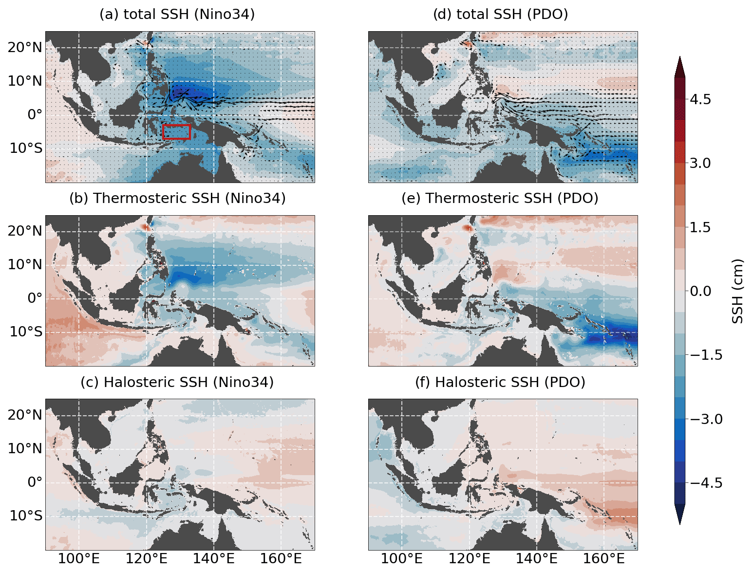
Figure 7Linear regression with the (a–c) Niño3.4 and (d–f) PDO index of upper-ocean currents (arrows; 0–150 m) for total, thermosteric, and halosteric SSH. All data are taken from REF005 and were filtered with an 8-year low-pass filter. Note that the colour shading in panels (a) and (b) is the same as in Fig. 5a and b.
The compensating effect of temperature and salinity changes during PDO cycles also manifests in the vertical profiles of temperature and salinity in the AMS. Figure 8 shows linear regressions of T and S averaged over the Banda Sea (7–3∘ S, 125–133∘ E: see red box in Fig. 7). Both hindcast experiments (Fig. 4a, b) indicate a strong negative subsurface response (hence the density compensation) to positive PDO cycles. The ENSO response is dominated by a subsurface temperature anomaly causing negative SSH values. The subsurface temperature anomalies during both ENSO and PDO cycles are amplified by sea surface salinity (SSS) anomalies. The two sensitivity experiments allow some insight into the origin of these surface signals (Fig. 4a, b). The momentum flux experiment (WIND) reproduces the subsurface signals, highlighting the fact that they are due to wind-stress-driven advection, but shows no surface anomalies associated with ENSO and PDO cycles. These are instead driven by buoyancy fluxes. This fits the ENSO-related halosteric anomalies (Fig. 7c) that do not seem to originate in the western tropical Pacific, but are instead forced by local buoyancy fluxes.
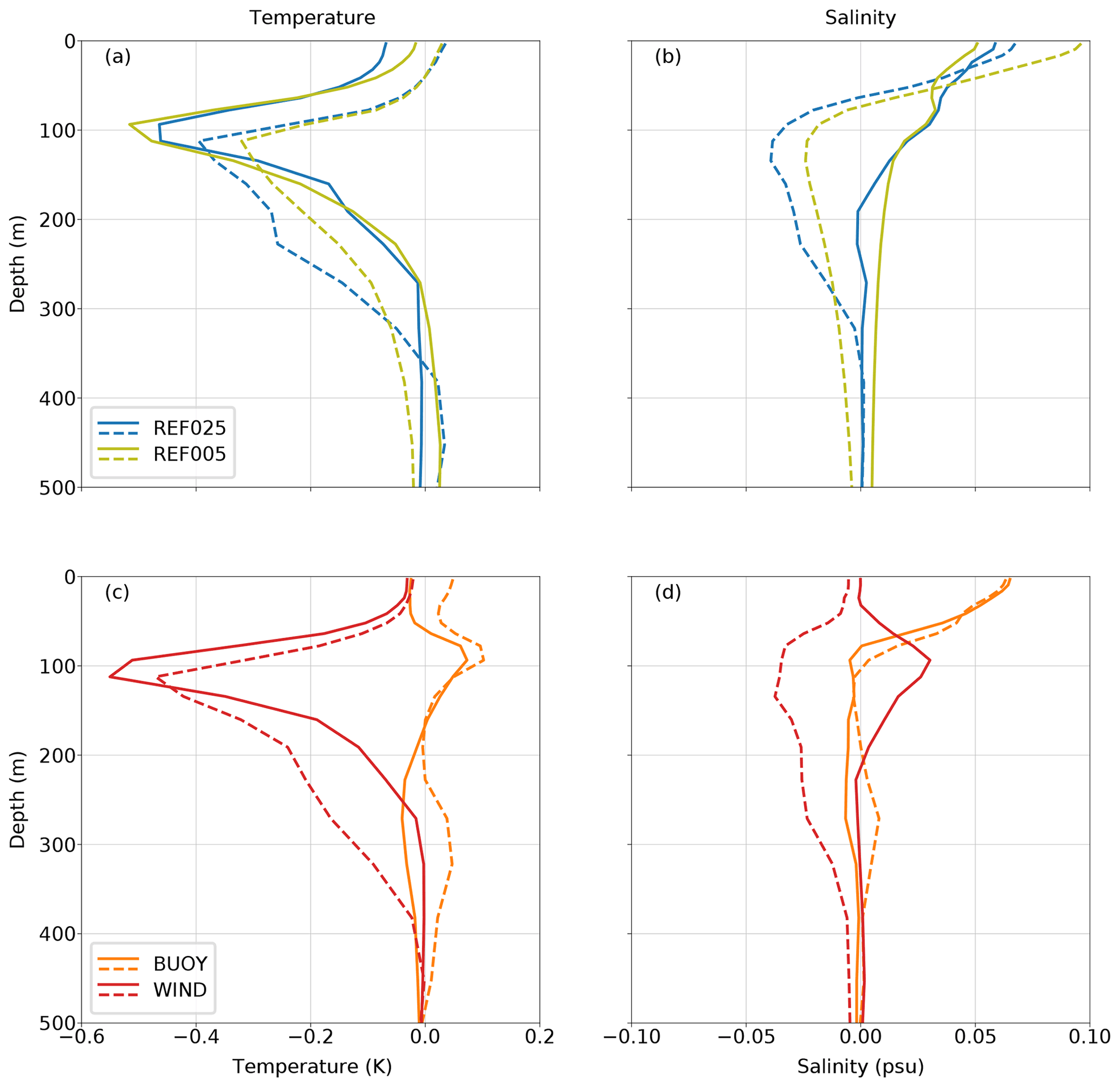
Figure 8Linear regression of temperature and salinity to the Niño3.4 (solid) and PDO index (dashed) from (a, b) reference experiments and (c, d) sensitivity experiments. All data have been filtered with an 8-year low-pass filter.
4.1 Summary
We determine the characteristics of decadal sea-level variability in the Australasian Mediterranean Sea and their relation to large-scale climate modes of ENSO and PDO by using a series of global ocean model experiments. Two reference configurations that resolve the area of interest with and ∘ horizontal resolution are set up and forced with the newly developed JRA-55 do forcing (Tsujino et al., 2018). Both simulations are able to reproduce observed sea-level variability in the western tropical Pacific and the AMS. We find minor resolution-dependent differences between the two simulations in terms of SSH. However, the coarse-resolution configuration suffers from some upper-ocean temperature and salinity biases, in particular in the northern part of the SCS and the Celebes Sea, which are alleviated in the high-resolution experiment.
We assess the regional fingerprints of ENSO and PDO on SSH in the region. Both climate modes produce strong sea-level signals in the western tropical Pacific. The ENSO-related signal is most pronounced just north of the Equator south of 10∘ N, which is in line with previous studies (e.g. Meng et al., 2019; Han et al., 2019). These strong SSH signals cause geostrophic flow anomalies as they change the inter-basin pressure gradient between the Pacific and the Indian Ocean and weaken the ITF (Hu et al., 2015). The imprint of the PDO in the northern part of the warm pool is weak and instead shifted southward. This confirms earlier reports which found the effect of the PDO (on multi-decadal timescales) in the western tropical Pacific to be most pronounced in the region of the SPCZ (Han et al., 2019; Moon et al., 2013; Becker et al., 2012). Our results suggest a partial compensation for thermosteric and halosteric PDO-related SSH anomalies. This is also in accordance with previous studies, which report a cooling and freshening of the southern part of the warm pool in response to a positive PDO cycle (Cravatte et al., 2009).
Within the AMS itself we find that, except for the central and northern SCS, over 80 % of the variability in the deep basins of the AMS is determined by low-frequency fluctuations of ENSO. The imprint of PDO cycles within the AMS is pronounced in the shallow Arafura and Timor seas as well as within the Java Sea, where it explains 20 % and 50 % of the total variability, respectively. Analysing sea-level trends since the early 90s from altimetry, tide gauge observations, and reconstructions, Strassburg et al. (2015) find similar results with respect to the PDO. Furthermore, our results suggest distinctly different patterns of variability related to ENSO and PDO in the SCS, where the ENSO pattern is limited to the northeastern part off the west coast of Luzon, and the PDO causes anomalies in the central SCS. This confirms previous results of idealized model studies (Cheng et al., 2016).
It can be expected that a clarification of the spatial pattern of multi-decadal variability will aid future projections of sea level in the region. With the recent phase shift of the PDO, the affected regions should be primed for a weakening of the recent sea-level rise, as is also observed in the western tropical Pacific (e.g. Hamlington et al., 2016; Piecuch et al., 2019).
In addition to two hindcast simulations, we set up a series of sensitivity experiments that used quasi-climatological forcing (Stewart et al., 2020) to remove interannual variability from the full forcing or only from the momentum or buoyancy fluxes. To our knowledge, the impact of buoyancy fluxes and intrinsic variability on regional sea level in the region has not been described in previous studies. Our results suggest that, even though momentum fluxes are the primary driver of variability, buoyancy fluxes are not negligible. According to our findings, they only contribute around 10 % on average to the total variability. However, this fraction is highly variable and can increase to up to 50 % during ENSO cycles when they amplify the wind-stress-driven sea-level anomalies. Indeed, buoyancy fluxes have been shown to be important for sea-level variability in other regions, including the tropical Pacific (Piecuch and Ponte, 2012; Ponte, 2012; Wagner et al., 2021). Intrinsic variability is relevant in the central SCS, where it accounts for 25 % of the low-frequency variability.
4.2 Discussion
We did not investigate the origin of the high levels of intrinsic variability in the SCS in detail and can only speculate at this point. A connection to mesoscale variability and the eddy-active Kuroshio region, which also shows high levels of intrinsic variability (Fig. 4e), seems likely. Both regions are connected via the Luzon Strait between Taiwan and the Philippines, and both regions show high levels of eddy kinetic energy (EKE; e.g. Scharffenberg and Stammer, 2010). Besides local (Wang et al., 2008) and remote (Chen et al., 2009; Cheng and Qi, 2010) wind forcing, the Luzon Strait transport (LST) has been identified in previous studies as driving interannual EKE variability in the SCS. An increased LST leads to a strengthening of the mean flow in the SCS, which creates favourable conditions for baroclinic instabilities that allow a downscale energy transfer (Sun et al., 2016). The strength of the LST is closely related to the Kuroshio current intrusion into the SCS (Qu et al., 2004; Wang and Fiedler, 2006) and the strength of the Kuroshio current itself. The Kuroshio current flows poleward along the western boundary, at which the Luzon Strait creates a gap through which the current can enter the SCS. The mechanisms that control the pathways and strength of this intrusion are complex and remain controversial (Nan et al., 2015, and references therein), but also include mechanisms by which eddies, generated by intrinsic variability in the Kuroshio region, impact the LST. While eddies are unlikely to cross the Luzon Strait directly, they have been observed to modulate the strength of the Kuroshio current (Jie and De-Hai, 2010), which could be a means by which intrinsic variability from the Kuroshio region is indirectly communicated into the SCS. However, the viability of this hypothesis and the determination of the mechanism involved need to be addressed in future research.
The aim of this study is to identify the deterministic low-frequency pattern of variability associated with large-scale climate modes. Although the separation of climate indices along timescales (ENSO: 8–13 years; PDO: > 13 years) is somewhat arbitrary, the results are not overly sensitive to the choice of the separation frequency. In fact, using only a low-pass-filtered ENSO index (> 8 years) yields results that are similar to the combined effect of bandpass-filtered ENSO and low-pass-filtered PDO we presented here. As already mentioned above, the PDO can be understood as the low-frequency component of ENSO in this context, and separating the timescales allowed us to show that the spatial pattern of SSH variability in the AMS and the mechanisms that drive it differ over these timescales.
An uncertainty of this study is the atmospheric forcing product used to drive the OGCMs. McGregor et al. (2012) demonstrated that most available atmospheric reanalyses, in conjunction with a linear shallow-water model, are able to reproduce the large-scale pattern of SSH variability in the Pacific, and we can confirm this for the dataset used here. However, we find minor biases in both reference configurations that are most likely due to the forcing. Hsu et al. (2021) report a wind stress curl bias in JRA55-do in the Pacific between 4 and 9∘ N that acts to diminish the meridional SSH gradient and flatten the SSH trough at this latitude. This is consistent with the warm bias we found at this latitudinal band. Also, consistent with the results found here, they further report an underestimation of SSH trends between 1993 and 2007 in the western tropical Pacific and relate it to an underestimation of the observed trade wind intensification.
A final point concerns the impact of model resolution in studies of variability patterns in this region. Although in our study we found only minor resolution-dependent differences between the and ∘ configurations with respect to SSH signals, the stronger biases in the temperature and salinity distributions seen in the coarser simulation should be taken as a reminder that a realistic representation of the dynamics of the AMS area, with its complex small-scale bathymetry, can require a very high model resolution. The importance of resolving the narrow straits and bathymetric details for capturing the ocean dynamics in the AMS was recently stressed in the review by Xue et al. (2020) of coupled ocean–atmosphere modelling for this region. In this context, it should be noted that the “coarse” ∘ grid used in this study would be in the higher-resolution category of current climate simulations with coupled ocean–atmosphere models, suggesting that projections of regional trend patterns in this area need to be interpreted with due caution. Downscaled projections (e.g. Sun et al., 2012; Feng et al., 2017), in which an uncoupled high-resolution OGCM is forced with a long-term climate change signal obtained from a climate model, might be a way to address this issue.
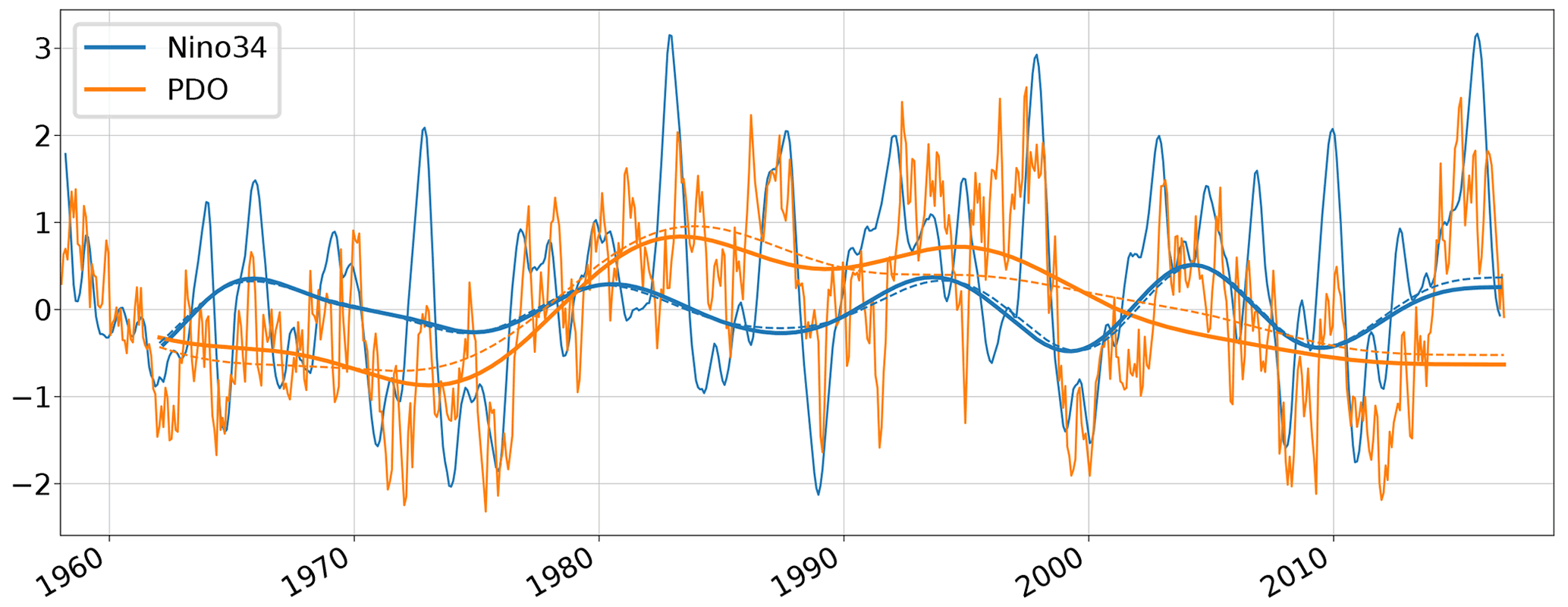
Figure A1Niño3.4 index and PDO index, both calculated from REF025. Smoothed lines are bandpass-filtered with cutoff periods of 8 and 13 years (Niño3.4) and low-pass-filtered with cutoff periods of 13 years (PDO). Dashed lines show observational estimates of the PDO index (http://research.jisao.washington.edu/pdo/PDO.latest, last access: 8 June 2017; Mantua et al., 1997) and the Niño3.4 index (https://psl.noaa.gov/gcos_wgsp/Timeseries/Data/nino34.long.data, last access: 7 June 2017; Rayner et al., 2003).

Figure A2Linear regression of SSH from WIND on the (a) Niño3.4 and (b) PDO index as well as the (c, d) respective coefficients of determination. Both climate indices are derived from REF025. All data were filtered with an 8-year low-pass filter.
Data shown in this paper are available at https://data.geomar.de/downloads/20.500.12085/e300e837-c02e-4939-a9b6-a9be163cbd26/ (Wagner and Böning, 2021).
PW and CWB defined the overall research problem and methodology; PW developed, ran, and validated the OGCM experiments; PW produced all figures; PW prepared the paper with contributions from CWB.
The contact author has declared that neither they nor their co-authors have any competing interests.
Publisher's note: Copernicus Publications remains neutral with regard to jurisdictional claims in published maps and institutional affiliations.
All model simulations have been performed at the North-German Supercomputing Alliance (HLRN). We thank Markus Scheinert for his contribution to the ocean model simulations used in this study. We thank Brett Buzzanga and two anonymous referees for their constructive comments.
This
research has been supported by the Deutsche Forschungsgemeinschaft as part of the Special Priority Programme (SPP) 1889 Regional Sea Level Change and Society (grant no. BO907/5-1).
The article processing charges for this open-access publication were covered by the GEOMAR Helmholtz Centre for Ocean Research Kiel.
This paper was edited by Erik van Sebille and reviewed by Brett Buzzanga and two anonymous referees.
Amante, C. and Eakins, B.: ETOPO1 1 Arc-Minute Global Relief Model: Procedures, Data Sources and Analysis. NOAA Technical Memorandum NESDIS NGDC-24, Tech. rep., National Geophysical Data Center, NOAA, https://doi.org/10.7289/V5C8276M, 2009. a
Barnier, B., Madec, G., Penduff, T., Molines, J. M., Treguier, A. M., Le Sommer, J., Beckmann, A., Biastoch, A., Böning, C., Dengg, J., Derval, C., Durand, E., Gulev, S., Remy, E., Talandier, C., Theetten, S., Maltrud, M., McClean, J., and De Cuevas, B.: Impact of partial steps and momentum advection schemes in a global ocean circulation model at eddy-permitting resolution, Ocean Dynam., 56, 543–567, https://doi.org/10.1007/s10236-006-0082-1, 2006. a
Becker, M., Meyssignac, B., Letetrel, C., Llovel, W., Cazenave, A., and Delcroix, T.: Sea level variations at tropical Pacific islands since 1950, Global Planet. Change, 80–81, 85–98, https://doi.org/10.1016/j.gloplacha.2011.09.004, 2012. a, b
Chen, G., Hou, Y., Chu, X., Qi, P., and Hu, P.: The variability of eddy kinetic energy in the South China Sea deduced from satellite altimeter data, Chin. J. Oceanol. Limn., 27, 943–954, https://doi.org/10.1007/s00343-009-9297-6, 2009. a
Cheng, X. and Qi, Y.: Trends of sea level variations in the South China Sea from merged altimetry data, Global Planet. Change, 57, 371–382, https://doi.org/10.1016/j.gloplacha.2007.01.005, 2007. a, b, c, d
Cheng, X. and Qi, Y.: Variations of eddy kinetic energy in the South China Sea, J. Oceanogr., 66, 85–94, https://doi.org/10.1007/s10872-010-0007-y, 2010. a
Cheng, X., Xie, S. P., Du, Y., Wang, J., Chen, X., and Wang, J.: Interannual-to-decadal variability and trends of sea level in the South China Sea, Clim. Dynam., 46, 3113–3126, https://doi.org/10.1007/s00382-015-2756-1, 2016. a, b, c, d, e
Clarke, A. J. and Liu, X.: Interannual Sea Level in the Northern and Eastern Indian Ocean, J. Phys. Oceanogr., 24, 1224–1235, https://doi.org/10.1175/1520-0485(1994)024<1224:ISLITN>2.0.CO;2, 1994. a
Cravatte, S., Delcroix, T., Zhang, D., McPhaden, M., and Leloup, J.: Observed freshening and warming of the western Pacific Warm Pool, Clim. Dynam., 33, 565–589, https://doi.org/10.1007/s00382-009-0526-7, 2009. a
Debreu, L., Vouland, C., and Blayo, E.: AGRIF: Adaptive grid refinement in Fortran, Comput. Geosci., 34, 8–13, https://doi.org/10.1016/j.cageo.2007.01.009, 2008. a
Fang, G., Chen, H., Wei, Z., Wang, Y., Wang, X., and Li, C.: Trends and interannual variability of the South China Sea surface winds, surface height, and surface temperature in the recent decade, J. Geophys. Res.-Oceans, 111, C11S16, https://doi.org/10.1029/2005JC003276, 2006. a
Feng, M., Li, Y., and Meyers, G.: Multidecadal variations of Fremantle sea level: Footprint of climate variability in the tropical Pacific, Geophys. Res. Lett., 31, L16302, https://doi.org/10.1029/2004GL019947, 2004. a
Feng, M., Böning, C., Biastoch, A., Behrens, E., Weller, E., and Masumoto, Y.: The reversal of the multi-decadal trends of the equatorial Pacific easterly winds, and the Indonesian Throughflow and Leeuwin Current transports, Geophys. Res. Lett., 38, L11604, https://doi.org/10.1029/2011GL047291, 2011. a
Feng, M., Benthuysen, J., Zhang, N., and Slawinski, D.: Freshening anomalies in the Indonesian throughflow and impacts on the Leeuwin Current during 2010–2011, Geophys. Res. Lett., 42, 8555–8562, https://doi.org/10.1002/2015GL065848, 2015. a
Feng, M., Zhang, X., Sloyan, B., and Chamberlain, M.: Contribution of the deep ocean to the centennial changes of the Indonesian Throughflow, Geophys. Res. Lett., 44, 2859–2867, https://doi.org/10.1002/2017GL072577, 2017. a, b
Fichefet, T. and Maqueda, M. A. M.: Sensitivity of a global sea ice model to the treatment of ice thermodynamics and dynamics, J. Geophys. Res.-Oceans, 102, 12609–12646, https://doi.org/10.1029/97JC00480, 1997. a
Forget, G. and Ponte, R. M.: The partition of regional sea level variability, Prog. Oceanogr., 137, 173–195, https://doi.org/10.1016/j.pocean.2015.06.002, 2015. a
Gordon, A. L.: Interocean exchange of thermocline water, J. Geophys. Res., 91, 5037–5046, https://doi.org/10.1029/jc091ic04p05037, 1986. a
Gordon, A. L.: Oceanography of the Indonesian seas and their throughflow, Oceanography, 18, 15–27, https://doi.org/10.5670/oceanog.2005.01, 2005. a
Hamlington, B. D., Cheon, S., Thompson, P. R., Merrifield, M. A., Nerem, R. S., Leben, R. R., and Kim, K.-Y.: An ongoing shift in Pacific Ocean sea level, J. Geophys. Res.-Oceans, 121, 5084–5097, https://doi.org/10.1002/2016JC011815, 2016. a
Han, W., Stammer, D., Thompson, P., Ezer, T., Palanisamy, H., Zhang, X., Domingues, C. M., Zhang, L., and Yuan, D.: Impacts of Basin-Scale Climate Modes on Coastal Sea Level: a Review, Surv. Geophys., 40, 1493–1541, https://doi.org/10.1007/s10712-019-09562-8, 2019. a, b
Hsu, C.-W., Yin, J., Griffies, S. M., and Dussin, R.: A mechanistic analysis of tropical Pacific dynamic sea level in GFDL-OM4 under OMIP-I and OMIP-II forcings, Geosci. Model Dev., 14, 2471–2502, https://doi.org/10.5194/gmd-14-2471-2021, 2021. a
Hu, D., Wu, L., Cai, W., Gupta, A. S., Ganachaud, A., Qiu, B., Gordon, A. L., Lin, X., Chen, Z., Hu, S., Wang, G., Wang, Q., Sprintall, J., Qu, T., Kashino, Y., Wang, F., and Kessler, W. S.: Pacific western boundary currents and their roles in climate, Nature, 522, 299–308, https://doi.org/10.1038/nature14504, 2015. a
International Hydrographic Organization: Limits of oceans and seas, 3rd Edition, Special Publication No. 23, Montecarlo, 1–42, 1953. a
Jie, Z. and De-Hai, L.: Response of the Kuroshio Current to Eddies in the Luzon Strait, Atmos. Ocean. Sci. Lett., 3, 160–164, https://doi.org/10.1080/16742834.2010.11446856, 2010. a
Kleinherenbrink, M., Riva, R., Frederikse, T., Merrifield, M., and Wada, Y.: Trends and interannual variability of mass and steric sea level in the Tropical Asian Seas, J. Geophys. Res.-Oceans, 122, 6254–6276, https://doi.org/10.1002/2017JC012792, 2017. a, b, c
Lee, T. and McPhaden, M. J.: Decadal phase change in large-scale sea level and winds in the Indo-Pacific region at the end of the 20th century, Geophys. Res. Lett., 35, L01605, https://doi.org/10.1029/2007GL032419, 2008. a
Liu, Q., Wang, D., Zhou, W., Xie, Q., and Zhang, Y.: Covariation of the Indonesian Throughflow and South China Sea Throughflow Associated with the 1976/77 Regime Shift, Adv. Atmos. Sci., 27, 87–94, https://doi.org/10.1007/s00376-009-8061-3, 2010. a
Liu, Q., Feng, M., and Wang, D.: ENSO-induced interannual variability in the southeastern South China Sea, J. Phys. Oceanogr., 67, 127–133, https://doi.org/10.1007/s10872-011-0002-y, 2011. a
Liu, Q.-Y., Feng, M., Wang, D., and Wijffels, S.: Interannual variability of the Indonesian Throughflow transport: A revisit based on 30 year expendable bathythermograph data, J. Geophys. Res.-Oceans, 120, 6405–6418, https://doi.org/10.1002/2015JC011351, 2015. a
Locarnini, R. A., Mishonov, A. V., Baranova, O. K., Boyer, T. P., Zweng, M. M., Garcia, H. E., Reagan, J. R., Seidov, D., Weathers, K. W., Paver, C. R., and Smolyar, I. V.: World Ocean Atlas 2018, Volume 1: Temperature, Tech. rep., NOAA, Silver Spring, available at: https://www.ncei.noaa.gov/sites/default/files/2021-03/woa18_vol1.pdf (last access: 18 October 2021), 2019. a
Madec, G. and NEMO-team: NEMO Ocean Engine, Tech. Rep. 27, Institut Pierre-Simon Laplace (IPSL), Paris, https://doi.org/10.5281/zenodo.1464816, 2016. a
Mantua, N. J., Hare, S. R., Zhang, Y., Wallace, J. M., and Francis, R. C.: A Pacific Interdecadal Climate Oscillation with Impacts on Salmon Production, B. Am. Meteorol. Soc., 78, 1069–1079, https://doi.org/10.1175/1520-0477(1997)078<1069:APICOW>2.0.CO;2, 1997. a
McGregor, S., Gupta, A. S., and England, M. H.: Constraining wind stress products with sea surface height observations and implications for Pacific Ocean sea level trend attribution, J. Climate, 25, 8164–9176, https://doi.org/10.1175/JCLI-D-12-00105.1, 2012. a, b
Meng, L., Zhuang, W., Zhang, W., Ditri, A., and Yan, X. H.: Decadal sea level variability in the Pacific Ocean: Origins and climate mode contributions, J. Atmos. Ocean. Tech., 36, 689–698, https://doi.org/10.1175/JTECH-D-18-0159.1, 2019. a
Merrifield, M. A.: A shift in western tropical Pacific sea level trends during the 1990s, J. Climate, 24, 4126–4138, https://doi.org/10.1175/2011JCLI3932.1, 2011. a
Merrifield, M. A. and Maltrud, M. E.: Regional sea level trends due to a Pacific trade wind intensification, Geophys. Res. Lett., 38, L21605, https://doi.org/10.1029/2011GL049576, 2011. a
Merrifield, M. A., Thompson, P. R., and Lander, M.: Multidecadal sea level anomalies and trends in the western tropical Pacific, Geophys. Res. Lett., 39, L3602, https://doi.org/10.1029/2012GL052032, 2012. a, b
Meyers, G.: Variation of Indonesian Throughflow and the El Nino-southern oscillation, J. Geophys. Res., 101, 212–255, 1996. a
Moon, J. H. and Song, Y. T.: Sea level and heat content changes in the western North Pacific, J. Geophys. Res.-Oceans, 118, 2014–2022, https://doi.org/10.1002/jgrc.20096, 2013. a
Moon, J. H., Song, Y. T., Bromirski, P. D., and Miller, A. J.: Multidecadal regional sea level shifts in the Pacific over 1958–2008, J. Geophys. Res.-Oceans, 118, 7024–7035, https://doi.org/10.1002/2013JC009297, 2013. a, b
Nan, F., Xue, H., and Yu, F.: Kuroshio intrusion into the South China Sea: A review, Prog. Oceanogr., 137, 314–333, https://doi.org/10.1016/j.pocean.2014.05.012, 2015. a
Peng, D., Palanisamy, H., Cazenave, A., and Meyssignac, B.: Interannual Sea Level Variations in the South China Sea Over 1950–2009, Mar. Geod., 36, 164–182, https://doi.org/10.1080/01490419.2013.771595, 2013. a
Piecuch, C. G. and Ponte, R. M.: Mechanisms of interannual steric sea level variability, Geophys. Res. Lett., 38, L15605, https://doi.org/10.1029/2011GL048440, 2011. a
Piecuch, C. G. and Ponte, R. M.: Buoyancy-driven interannual sea level changes in the southeast tropical Pacific, Geophys. Res. Lett., 39, 1–5, https://doi.org/10.1029/2012GL051130, 2012. a
Piecuch, C. G., Thompson, P. R., and Hamlington, B. D.: What Caused Recent Shifts in Tropical Pacific Decadal Sea-Level Trends?, J. Geophys. Res.-Oceans, 124, 7575–7590, https://doi.org/10.1029/2019JC015339, 2019. a, b
Ponte, R. M.: An assessment of deep steric height variability over the global ocean, Geophys. Res. Lett., 39, L04601, https://doi.org/10.1029/2011GL050681, 2012. a
Qiu, B. and Chen, S.: Multidecadal Sea Level and Gyre Circulation Variability in the Northwestern Tropical Pacific Ocean, J. Phys. Oceanogr., 42, 193–206, https://doi.org/10.1175/JPO-D-11-061.1, 2012. a
Qu, T., Kim, Y. Y., Yaremchuk, M., Tuzuka, T., Ishida, A., and Yamagata, T.: Can Luzon Strait transport play a role in conveying the impact of ENSO to the South China Sea?, J. Climate, 17, 3644–3657, https://doi.org/10.1175/1520-0442(2004)017<3644:CLSTPA>2.0.CO;2, 2004. a
Rayner, N. A., Parker, D. E., Horton, E. B., Folland, C. K., Alexander, L. V., Rowell, D. P., Kent, E. C., and Kaplan, A.: Global analyses of sea surface temperature, sea ice, and night marine air temperature since the late nineteenth century, J. Geophys. Res.-Atmos., 108, 4407, https://doi.org/10.1029/2002jd002670, 2003. a
Rong, Z., Liu, Y., Zong, H., and Cheng, Y.: Interannual sea level variability in the South China Sea and its response to ENSO, Global Planet. Change, 55, 257–272, https://doi.org/10.1016/j.gloplacha.2006.08.001, 2007. a, b, c
Ryan, S., Ummenhofer, C. C., Gawarkiewicz, G., Wagner, P., Scheinert, M., Biastoch, A., and Böning, C. W.: Depth structure of Ningaloo Niño/Niña events and associated drivers, J. Climate, 34, 1767–1788, https://doi.org/10.1175/jcli-d-19-1020.1, 2021. a
Saji, N. H., Goswami, B. N., Vinayachandran, P. N., and Yamagata, T.: A dipole mode in the tropical Indian Ocean, Nature, 401, 360–363, https://doi.org/10.1038/43854, 1999. a, b
Scharffenberg, M. G. and Stammer, D.: Seasonal variations of the large-scale geostrophic flow field and eddy kinetic energy inferred from the TOPEX/Poseidon and Jason-1 tandem mission data, J. Geophys. Res.-Oceans, 115, C02008, https://doi.org/10.1029/2008JC005242, 2010. a
Schwarzkopf, F. U., Biastoch, A., Böning, C. W., Chanut, J., Durgadoo, J. V., Getzlaff, K., Harlaß, J., Rieck, J. K., Roth, C., Scheinert, M. M., and Schubert, R.: The INALT family – a set of high-resolution nests for the Agulhas Current system within global NEMO ocean/sea-ice configurations, Geosci. Model Dev., 12, 3329–3355, https://doi.org/10.5194/gmd-12-3329-2019, 2019. a
Sprintall, J., Gordon, A. L., Koch-Larrouy, A., Lee, T., Potemra, J. T., Pujiana, K., Wijffels, S. E., and Wij, S. E.: The Indonesian seas and their role in the coupled ocean–climate system, Nat. Geosci., 7, 487–492, https://doi.org/10.1038/ngeo2188, 2014. a
Stewart, K. D., Kim, W. M., Urakawa, S., Hogg, A. M. C., Yeager, S., Tsujino, H., Nakano, H., Kiss, A. E., and Danabasoglu, G.: JRA55-do-based repeat year forcing datasets for driving ocean–sea-ice models, Ocean Model., 147, 1–27, https://doi.org/10.1016/j.ocemod.2019.101557, 2020. a, b
Strassburg, M. W., Hamlington, B. D., Leben, R. R., Manurung, P., Lumban Gaol, J., Nababan, B., Vignudelli, S., and Kim, K.-Y.: Sea level trends in Southeast Asian seas, Clim. Past, 11, 743–750, https://doi.org/10.5194/cp-11-743-2015, 2015. a, b, c, d
Sun, C., Feng, M., Matear, R. J., Chamberlain, M. A., Craig, P., Ridgway, K. R., and Schiller, A.: Marine downscaling of a future climate scenario for Australian boundary currents, J. Climate, 25, 2947–2962, https://doi.org/10.1175/JCLI-D-11-00159.1, 2012. a
Sun, Z., Zhang, Z., Zhao, W., and Tian, J.: Interannual modulation of eddy kinetic energy in the northeastern South China Sea as revealed by an eddy-resolving OGCM, J. Geophys. Res.-Oceans, 121, 3190–3201, https://doi.org/10.1002/2015JC011497, 2016. a
Thomson, R. and Emery, W.: Data Analysis Methods in Physical Oceanography, Elsevier Science, 3 edn., Amsterdam, 2014. a
Timmermann, A., McGregor, S., and Jin, F. F.: Wind effects on past and future regional sea level trends in the southern Indo-Pacific, J. Climate, 23, 4429–4437, https://doi.org/10.1175/2010JCLI3519.1, 2010. a
Tomczak, M. and Godfrey, J. S.: Regional Oceanography: an Introduction, Daya Publishing House, Delhi, 2 edn., 2003. a
Tsujino, H., Urakawa, S., Nakano, H., Small, R. J., Kim, W. M., Yeager, S. G., Danabasoglu, G., Suzuki, T., Bamber, J. L., Bentsen, M., Böning, C. W., Bozec, A., Chassignet, E. P., Curchitser, E., Boeira Dias, F., Durack, P. J., Griffies, S. M., Harada, Y., Ilicak, M., Josey, S. A., Kobayashi, C., Kobayashi, S., Komuro, Y., Large, W. G., Le Sommer, J., Marsland, S. J., Masina, S., Scheinert, M., Tomita, H., Valdivieso, M., and Yamazaki, D.: JRA-55 based surface dataset for driving ocean–sea-ice models (JRA55-do), Ocean Model., 130, 79–139, https://doi.org/10.1016/j.ocemod.2018.07.002, 2018. a, b
Ummenhofer, C. C., Ryan, S., England, M. H., Scheinert, M., Wagner, P., Biastoch, A., and Böning, C. W.: Late 20th Century Indian Ocean Heat Content Gain Masked by Wind Forcing, Geophys. Res. Lett., 47, e2020GL088692, https://doi.org/10.1029/2020GL088692, 2020. a
Wagner, P. and Böning, C. W.: Supplementary Data to “Decadal sea-level variability in the Australasian Mediterranean Sea”, GEOMAR [supplementary data set], available at: https://data.geomar.de/downloads/20.500.12085/e300e837-c02e-4939-a9b6-a9be163cbd26/, last access: 18 October 2021. a
Wagner, P., Scheinert, M., and Böning, C. W.: Contribution of buoyancy fluxes to tropical Pacific sea level variability, Ocean Sci., 17, 1103–1113, https://doi.org/10.5194/os-17-1103-2021, 2021. a, b, c
Wainwright, L., Meyers, G., Wijffels, S., and Pigot, L.: Change in the Indonesian Throughflow with the climatic shift of 1976/77, Geophys. Res. Lett., 35, L03604, https://doi.org/10.1029/2007GL031911, 2008. a
Wang, C. and Fiedler, P. C.: ENSO variability and the eastern tropical Pacific: A review, Prog. Oceanogr., 69, 239–266, https://doi.org/10.1016/j.pocean.2006.03.004, 2006. a
Wang, G., Chen, D., and Su, J.: Winter eddy genesis in the eastern South China Sea due to orographic wind jets, J. Phys. Oceanogr., 38, 726–732, https://doi.org/10.1175/2007JPO3868.1, 2008. a
Wijffels, S. and Meyers, G.: An Intersection of Oceanic Waveguides: Variability in the Indonesian Throughflow Region, J. Phys. Oceanogr., 34, 1232–1253, https://doi.org/10.1175/1520-0485(2004)034<1232:AIOOWV>2.0.CO;2, 2004. a, b
Wu, C. R. and Chang, C. W.: Interannual variability of the South China Sea in a data assimilation model, Geophys. Res. Lett., 32, L17611, https://doi.org/10.1029/2005GL023798, 2005. a
Xue, P., Malanotte-Rizzoli, P., Wei, J., and Eltahir, E. A.: Coupled Ocean-Atmosphere Modeling Over the Maritime Continent: A Review, J. Geophys. Res.-Oceans, 125, e2019JC014978, https://doi.org/10.1029/2019JC014978, 2020. a
Zhuang, W., Qiu, B., and Du, Y.: Low-frequency western Pacific Ocean sea level and circulation changes due to the connectivity of the Philippine archipelago, J. Geophys. Res.-Oceans, 118, 6759–6773, https://doi.org/10.1002/2013JC009376, 2013. a, b
Zweng, M. M., Reagan, J. R., Seidov, D., Boyer, T. P., Antonov, J. I., Locarnini, R. A., Garcia, H. E., Mishonov, A. V., Baranova, O. K., Weathers, K. W., Paver, C. R., and Smolyar, I. V.: World Ocean Atlas 2018, Volume 2: Salinity, Tech. Rep. 82, NOAA, Silver Spring, 2019. a
We will refer to the sea-level estimate of the OGCMs, which gives height above the geoid, as SSH.
The Niño3.4 index is defined as the area-averaged sea surface temperature (SST) anomaly in the Niño3.4 region (5∘ N–5∘ S, 170–120∘ W) with respect to the monthly climatology normalized by its SD.
The PDO index is obtained via an empirical orthogonal function of monthly SST anomalies in the Pacific north of 20∘ N and defined as the leading mode of variability. The climatological annual cycle is subtracted to remove long-term trends.