the Creative Commons Attribution 4.0 License.
the Creative Commons Attribution 4.0 License.
 | 19 Jan 2021
Accuracy assessment of global internal-tide models using satellite altimetry
Loren Carrere
Brian K. Arbic
Brian Dushaw
Gary Egbert
Svetlana Erofeeva
Florent Lyard
Richard D. Ray
Clément Ubelmann
Edward Zaron
Zhongxiang Zhao
Jay F. Shriver
Maarten Cornelis Buijsman
Nicolas Picot
Altimeter measurements are corrected for several geophysical parameters in order to access ocean signals of interest, like mesoscale or sub-mesoscale variability. The ocean tide is one of the most critical corrections due to the amplitude of the tidal elevations and to the aliasing phenomena of high-frequency signals into the lower-frequency band, but the internal-tide signatures at the ocean surface are not yet corrected globally.
Internal tides can have a signature of several centimeters at the surface with wavelengths of about 50–250 km for the first mode and even smaller scales for higher-order modes. The goals of the upcoming Surface Water Ocean Topography (SWOT) mission and other high-resolution ocean measurements make the correction of these small-scale signals a challenge, as the correction of all tidal variability becomes mandatory to access accurate measurements of other oceanic signals.
In this context, several scientific teams are working on the development of new internal-tide models, taking advantage of the very long altimeter time series now available, which represent an unprecedented and valuable global ocean database. The internal-tide models presented here focus on the coherent internal-tide signal and they are of three types: empirical models based upon analysis of existing altimeter missions, an assimilative model and a three-dimensional hydrodynamic model.
A detailed comparison and validation of these internal-tide models is proposed using existing satellite altimeter databases. The analysis focuses on the four main tidal constituents: M2, K1, O1 and S2. The validation process is based on a statistical analysis of multi-mission altimetry including Jason-2 and Cryosphere Satellite-2 data. The results show a significant altimeter variance reduction when using internal-tide corrections in all ocean regions where internal tides are generating or propagating. A complementary spectral analysis also gives some estimation of the performance of each model as a function of wavelength and some insight into the residual non-stationary part of internal tides in the different regions of interest. This work led to the implementation of a new internal-tide correction (ZARON'one) in the next geophysical data records version-F (GDR-F) standards.
- Article
(31237 KB) - Full-text XML
-
Supplement
(1195 KB) - BibTeX
- EndNote


Since the early 1990s, several altimeter missions have been monitoring sea level at a global scale, nowadays offering a long and very accurate time series of measurements. This altimetry database is nearly homogeneous over the entire ocean, allowing the sampling of many regions that were poorly sampled or not sampled at all before the satellite era. Thanks to its current accuracy and maturity, altimetry is now regarded as a fully operational observing system dedicated to ocean and climate applications (Escudier et al., 2017).
The main difficulty encountered when using altimeter datasets for ocean studies is related to the long revisit time of the satellites, which results in the aliasing of high-frequency ocean signals into a much lower-frequency band. Concerning tidal frequencies, the 9.9156 d cycle of TOPEX/Poseidon and Jason altimeter series induces the aliasing of the semidiurnal M2 lunar tide into a 62 d period, and the diurnal K1 tide is aliased into a 173 d period, the latter of which is very close to the semiannual frequency and raises complex separation problems. The long duration of the global ocean altimeter database available has allowed the community to overcome this separation problem, and new global ocean barotropic tidal solutions (Stammer et al., 2014) have been produced taking advantage of altimeter data: among them the last Goddard/Grenoble Ocean Tide model (denoted GOT: Ray, 2013) and the last finite-element solution for ocean tide (denoted FES2014: Carrere et al., 2016a; Lyard et al., 2020), which are commonly used as reference for the barotropic tide correction in actual altimeter geophysical data records (denoted GDRs). Moreover this altimeter database has been used in numerous studies to validate new instrumental and geophysical corrections used in altimetry, thanks to the analysis of their impact on the sea level estimation at climate scales, as well as at lower temporal scales like mesoscale signals; in particular, it has proven its efficiency for validating global ocean models (Shum 1997; Stammer et al., 2014; Carrere et al., 2016b; Quartly et al., 2017).
The upcoming Surface Water Ocean Topography (SWOT) mission, led by NASA, CNES, and the UK and Canadian space agencies, is planned for 2021 and will measure sea surface height with a spatial resolution never proposed before, thus raising the importance of the correction of the internal-tide surface signature. Internal tides (denoted ITs) are generated by an incoming barotropic tidal flow on a bathymetric pattern within a stratified ocean and can have amplitudes of several tens of meters at the thermocline level and a signature of several centimeters at the surface, with wavelengths ranging approximately between 30 and 250 km for the lowest three modes of variability (Chelton et al., 1998). From the perspective of the SWOT mission and of high-resolution ocean measurements in general, removing these small-scale surface signals is a challenge because we need to be able to separate all tidal signals to access other oceanic variability of interest such as mesoscale, sub-mesoscale or climate signals.
A large part of the internal-tide signal remains coherent over long times, with large stable propagation patterns across ocean basins, such as the North Pacific and many other regions (Dushaw et al., 2011). The amplitude of the coherent signal appears to be greatly diminished in the equatorial regions, which may be caused by the direct disrupting effect of the rapid equatorial wave variations (Buijsman et al., 2017) or merely masked by the background noise. The seasonal variability of the ocean medium and the interaction with mesoscale eddies and currents may also disrupt the coherence of the internal tide in many other areas, which makes the non-coherent internal tides' variability more complex to observe and model (Shriver et al., 2014).
In this context, and since conventional satellite altimetry has already shown its ability to detect small-scale internal-tide surface signatures (Ray and Mitchum, 1997; Dushaw 2002; Carrere et al., 2004), several scientific teams have developed new internal-tide models, taking advantage of the very long altimeter time series now available. These internal-tide models are of three types: empirical models based upon analysis of existing altimeter missions, usually more than one; assimilative models based upon assimilating altimeter data into a reduced-gravity model; and three-dimensional hydrodynamic models, which embed internal tides into an eddying general circulation model. In the present paper, the analysis is focused on seven models that yield a coherent internal-tide solution: Dushaw (2015), Egbert and Erofeeva (2014), Ray and Zaron (2016), Shriver et al. (2014), Clément Ubelmann (personal communication, 2017), Zaron (2019), and Zhao et al. (2016, 2019a).
The objective of this paper is to present a detailed comparison and a validation assessment of these internal-tide models using satellite altimetry. The present analysis focuses on the coherent internal-tide signal for the main tidal constituents: M2, S2, K1 and O1. The validation process is based on a statistical analysis and on a comparison to multi-mission altimetry including Jason-2 (denoted J2 hereafter) and Cryosphere Satellite-2 (also named CryoSat-2 or C2 hereafter) LRM data (low-resolution mode). For the sake of clarity, only results for the main tidal components M2 and K1 are presented in the core of this paper, and O1 and S2 validation results are gathered in the Appendix.
After a brief description of the participating models (Sect. 2), an analysis of the differences between internal-tide models is presented in Sect. 3. Section 4 describes the altimeter dataset used, the method of comparison and the validation strategy. The validation results of the different internal-tide corrections versus altimetry databases are described in Sects. 5 and 6. Finally, a discussion and concluding remarks are gathered in Sect. 7.
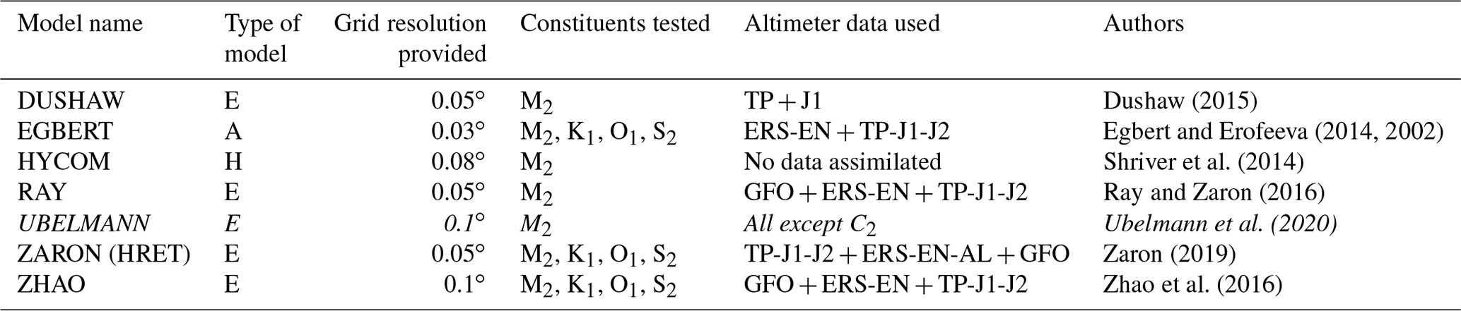
This section gives a brief overview of the internal-tide models evaluated in this study. We considered five purely empirical models involving data merging, one data assimilative model and also one pure hydrodynamic model simulating tides and internal tides using the gravitational forcing and a high spatial resolution but without any internal-tide data constraint. The list of participating IT models is given in Table 1.
Table 1List of the participating IT models. Most of the models are global models except one that is currently available in only two areas (Hawaii and Azores, noted in italic). E – empirical model; A – assimilative model; H – hydrodynamic model. Abbreviations used for altimeter missions: TP – TOPEX/Poseidon; J1 – Jason-1; J2 – Jason-2; EN – Envisat; GFO – GEOSAT Follow-On; C2 – CryoSat-2; AL – AltiKa.
2.1 Empirical models
The purely empirical models are based upon the analysis of existing conventional altimeter missions, usually more than one. The five empirical models used in the present study are briefly described below.
DUSHAW
This global model was computed using a frequency–wavenumber tidal analysis (Dushaw et al., 2011; Dushaw, 2015). The internal tides were assumed to be composed of narrow-band spectra of traveling waves, and these waves are fitted to the altimeter data in both time and position. A tidal analysis of a time series allows extracting accurate tidal estimates from noisy or irregular data under the assumptions that the signal is temporally coherent and described by a few known frequencies. The frequency–wavenumber analysis generalizes such an analysis to include the spatial dimension, making the strong assumptions that both time and spatial wave variations are coherent. In addition to the known tidal constituent frequencies, the solution also requires accurate values for the local intrinsic wavelengths of low-mode internal waves. Internal-tide properties, which depend on inertial frequency, stratification and depth, were derived using the 2009 World Ocean Atlas (Antonov et al., 2010; Locarnini et al., 2010) and Smith and Sandwell global seafloor topography (Smith and Sandwell, 1997). The solution is a spectral model with no inherent grid resolution; tidal quantities of interest derived from the solution are both inherently consistent with the data employed and influenced by non-local data.
The fit used M2, S2, N2, K2, O1 and K1 constituents, with spectral bands for barotropic, mode-1 and mode-2 wavenumbers. Data from the TOPEX/Poseidon (TP) and Jason-1 altimetry programs were employed. These data had the barotropic tides removed, but the fit allowed for residual barotropic variations. Employing all constituents and wavelengths simultaneously in a single fit minimized the chance that the solution for a particular constituent was influenced by noise from nearby tidal constituents. To account for regional variations in the internal-tide characteristics (and reduce computational cost) independent fits were made in 11∘ × 11∘ overlapping regions. The global solution was obtained by merging the regional solutions together using a cosine taper over a 1∘ interval; the solution is therefore sometimes discontinuous within these overlapping zones. For this study, global maps of the harmonic constants for the two first baroclinic modes of the largest semidiurnal tidal constituent M2 were computed on a regular 1∕20∘ grid (Dushaw, 2015; the complete solution is available from http://www.apl.washington.edu/project/project.php?id=tm_1-15, last access: 17 December 2020). This global M2 solution was tested against pointwise, along-track estimates for the internal tide, with satisfactory comparisons in the Atlantic and Pacific oceans. Comparisons were also made to in situ measurements by ocean acoustic tomography in the Pacific and Atlantic, showing a good predictability in both amplitude and phase. By comparisons to the tomography data, internal tides within the Philippine Sea (Dushaw, 2015) or Canary Basin (Dushaw et al., 2017) were less predictable. Some of these comparisons found good agreement between hindcasts and time series recorded in the western North Atlantic about a decade before the altimetry data were available, which is consistent with the extraordinary temporal coherence of this IT signal in many regions of the world's oceans.
RAY
The RAY model provides a global chart of surface elevations associated with the stationary M2 internal-tide signal. This map is empirically constructed from multi-mission satellite altimeter data, including GFO (GEOSAT Follow-On), ERS (European Remote Sensing satellite), Envisat, TOPEX/Poseidon, and the J1 and J2 missions. Although the present-day altimeter coverage is not entirely adequate to support a direct mapping of very short-wavelength features such as surface internal-tide signatures, using an empirical mapping approach produces a model that is independent of any assumption about ocean wave dynamics. The along-track data from each satellite mission were subjected to tidal analysis, and the M2 fields were high-pass-filtered to remove residual noise from barotropic and other long-wavelength modeling errors. Filtered data from all mission tracks were then interpolated to a regular grid. The complete description of the methodology is described in Ray and Zaron (2016, Sect. 3). Validation using some independent data from CryoSat-2 showed a positive variance reduction in most areas except in regions of large mesoscale variability, due to some contamination from non-tidal ocean variability in these last regions (Ray and Zaron, 2016). In the model version used in the present study, those regions have been masked with a taper to give zero elevation. The model grid has a 1∕20∘ resolution and it is defined over the 50∘ S–60∘ N latitude band.
UBELMANN
The internal-tide solution is obtained from all altimetry satellites in the period 1990–2013, except for the CryoSat-2 mission. The method relies on a simultaneous estimation of the mesoscales and coherent M2 internal tides. Indeed, the mesoscale signal is known to introduce errors in the tidal estimation (non-zero harmonics in a finite time window). To mitigate that issue, most existing methods subtract the low-frequency altimetry field from AVISO (Archiving, Validation and Interpretation of Satellite Oceanographic data) as a proxy for mesoscales (e.g., Ray and Zaron, 2016). However, the estimate of the mesoscale is itself contaminated by internal tides (e.g., Zaron and Ray, 2018) aliased into a low frequency, which also introduces errors. For these reasons, Clément Ubelmann (personnal communication, 2017) proposed here a simultaneous estimation, accounting for the covariances of mesoscales and internal tides in a single inversion. In practice, these covariances are expressed as a reduced wavelet basis (local in time and space) for mesoscales and as a plane wave basis (local in space only) for internal tides. The plane wave wavelength and phase speed rely on the first and second Rossby radii of deformation climatology by Chelton et al. (1998). Although the inversion cannot be done explicitly (because of the long time window extending the basis size for the mesoscale), a variational minimization allows for a converged solution after about 100 iterations (typical degree of freedom for the problem). For this study, only the M2 internal-tide solution (for mode 1 and mode 2) is considered, but the mesoscale solution is also of interest because the internal-tide contamination should be minimized compared to the standard AVISO processing.
The method is further described in Ubelmann et al. (2020). Further improvements are expected after introducing additional tide components in the same inversion and after considering slow (or seasonal) variation in the phases.
ZARON
The High Resolution Empirical Tide (HRET) model provides an empirical estimate for the baroclinic tides at the M2, S2, K1 and O1 frequencies, as well as the annual modulations of M2, denoted MA2 and MB2. The development of HRET begins with assembling time series of essentially all the exact-repeat mission altimetry along the reference and interleaved orbit ground tracks of the TOPEX/Poseidon–Jason missions, the ERS–Envisat–AltiKa missions and the GEOSAT Follow-On mission (Zaron, 2019). Standard atmospheric path delay and environmental corrections are applied to the data, including the removal of the barotropic tide using the GOT4.10c model and the removal of an estimate for the mesoscale sea level anomaly using a purpose-filtered version of the Ssalto/Duacs multi-mission L4 sea level anomaly product (Zaron and Ray, 2018). Conventional harmonic analysis is then used to compute harmonic constants at each point along the nominal 1 Hz ground tracks (Carrere et al., 2004), and these data are used as inputs for subsequent steps.
HRET was initially developed to evaluate plausible spatial models for the baroclinic tides, seeking ways to improve on some previous models (Zhao et al., 2012; Ray and Zaron, 2016). It uses a local representation of the wave field as a sum of waves modulated by an amplitude envelope consisting of a second-order polynomial, thus generalizing the spatial signal model used in previous plane wave fitting (Ray and Mitchum, 1997; Zhao et al., 2016). The details of the implementation in HRET differ in additional ways from previous approaches. Specifically, the wavenumber modulus and direction of each wave component are determined by local two-dimensional Fourier analysis of the along-track data, and the coefficients in the spatial model are determined by weighted least-squares fitting to along-track slope data – the latter removes the need for rather arbitrary along-track high-pass filtering used in other estimates. Hence, the model is fully empirical in the sense that it does not use an a priori wavenumber dispersion relation.
The above-described approach to building local models for the baroclinic waves is applied to overlapping patches of the ocean, which are then blended and smoothly interpolated on a uniform latitude–longitude grid. Using the standard error estimates from the original harmonic analysis and goodness-of-fit information from the spatial models, a mask is prepared which smoothly damps the model fields to zero in regions where the estimate is believed to be too noisy to be useful. These are generally regions near the coastline where the number of data used are reduced or regions in western boundary currents or the Southern Ocean where the baroclinic tides cannot be distinguished from the continuum of energetic mesoscale variability. HRET version 7.0 was provided for the present validation analysis. Note that the model is still being refined and version 8.1 is available at present: it has improved O1 relative to the results shown here and made minor changes to the other constituents.
ZHAO
This model is constructed by a two-dimensional plane wave fit method (Zhao et al., 2016). In this method, internal tidal waves are extracted by fitting plane waves using SSH (sea surface height) measurements in individual fitting windows (160 km by 160 km for M2). Prerequisite wavenumbers are calculated using climatological ocean stratification profiles. For each window, the amplitude and phase of one plane wave in each compass direction (angular increment 1∘) are determined by the least-squares fit. When the fitted amplitudes are plotted as a function of direction in polar coordinates, an internal tidal wave appears to be a lobe. The largest lobe gives the amplitude and direction of one internal tidal wave. The signal of the determined wave is predicted and removed from the initial SSH measurements. This procedure can be repeated to extract an arbitrary number of waves (three waves here). Four tidal constituents M2, S2, O1 and K1 are mapped separately using their respective parameters and are used in the present paper (model version Zhao16). This mapping technique dynamically interpolates internal tidal waves at off-track sites using neighboring on-track measurements, overcoming the difficulty posed by widely spaced ground tracks. There are a large number of independent SSH measurements in each fitting window, compared to a single time series of SSH measurements used by pointwise harmonic analysis. As a result, non-tidal noise caused by tidal aliasing can be efficiently suppressed. This technique resolves multiple waves of different propagation directions; therefore, the decomposed internal-tide fields may provide more information on generation and propagation.
2.2 Assimilative model
Gary D. Egbert and Svetlana Y. Erofeeva have developed a reduced-gravity (RG) data assimilation scheme for mapping low-mode coherent internal tides (Egbert and Erofeeva, 2014) and applied this to a multi-mission dataset to produce global first mode M2 and K1 solutions. This scheme is based on the Boussinesq linear equations for flow over arbitrary topography with a free surface and horizontally uniform stratification. As in Tailleux and McWilliams (2001) and Griffiths and Grimshaw (2007), vertical dependence of the flow variables are described using flat-bottom modes (which depend on the local depth H(x,y)), yielding a coupled system of (two-dimensional) partial differential equations (PDEs) for the modal coefficients for surface elevation and horizontal velocity. Equations for each mode are coupled through interaction coefficients, which can be given in terms of the vertical-mode eigenvalues following the approach of Griffiths and Grimshaw (2007). Modes are decoupled wherever bathymetric gradients are zero, and for a flat bottom the system reduces to the usual single-mode RG shallow-water equations.
Within the RG scheme used, the vertical-mode coupling terms are dropped to obtain independent equations for the propagation of each mode with spatially variable reduced water depth, which are determined from local bathymetry and stratification. These simplified equations are identical to the linear shallow-water equations used in the OSU Tidal Inversion Software (OTIS, https://www.tpxo.net/otis, last access: 17 December 2020; Egbert and Erofeeva, 2002), thus allowing the use of the assimilation system to map internal tides by simply modifying depth and fitting along-track harmonic constants as a sum over a small number of modes. With some extensions to OTIS, coupling terms for the first few modes can be included in the dynamics.
This OTIS-RG assimilation scheme has been applied to construct global maps of first mode temporally coherent internal-tide elevations. Available exact repeat mission data, except GFO, were assimilated (TP-Jason, ERS/Envisat), with the AVISO weekly gridded SSH product used to reduce mesoscale variations before harmonic analysis. Solutions are computed in overlapping patches (∼ 20∘ × 30∘) and then merged (via weighted average on overlaps) into a global solution. It may be noted that adjacent solutions almost always match quite well even without this explicit tapering.
2.3 Hydrodynamic model
The hydrodynamic internal-tide solution is provided by the three-dimensional ocean model HYCOM (HYbrid Coordinate Ocean Model), which embeds tides and internal tides into an eddying general circulation model (Shriver et al., 2014). A free simulation, i.e., without any data assimilation, is used for the present study; this run used an augmented state ensemble Kalman filter (ASEnKF) to correct the forcing and reduce the M2 barotropic tidal error to about 2.6 cm (Ngodock et al., 2016). The value of such a simulation is to provide some information about the interaction of internal tides with mesoscales and other oceanic signals in addition to the internal-tide signal itself, which means that it can give access to the non-coherent internal-tide signal too. For the present study, a 1-year simulation (simulation no. 102 on year 2014) has been run and a harmonic analysis of the steric 1 h SSH allowed the extraction of the M2 internal-tide signal which remains coherent in this period. The non-assimilative quality of the simulation makes it entirely independent from the altimeter database used for the validation. The spatial resolution of the native grid is 1∕24∘, but data have been interpolated on a 1∕12.5∘ grid to provide the tidal atlas for the present analysis.
3.1 Qualitative comparison of IT elevations
A first analysis of the model differences consists in visualizing the patterns of IT models' amplitude in the regions of interest defined in Fig. 1. These seven regions are characterized by a well-known and nearly permanent internal-tide signal, already pointed out by previous studies (Egbert et al., 2000; Carrere et al., 2004; Nugroho, 2017). From the seven regions of interest, the North Pacific area (NPAC) and Luzon regions were selected for the comparison hereafter because they are more energetic regions; moreover, all tested models are available in the NPAC region and the Luzon area is characterized by strong semidiurnal and diurnal baroclinic tides.
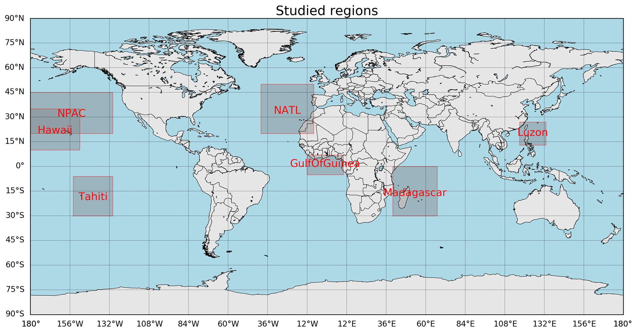
Figure 1Localization of the internal-tide regions studied in the present paper.
Figure 2 shows the M2 IT amplitude of each model in the NPAC located around the Hawaiian islands. In this region, all models have similar amplitudes and similar beam patterns demonstrating northeastward propagation with one clear northward beam; amplitudes are often greater than 2 cm. The amplitude's pattern varies along IT beams with short spatial scales, indicating that most of the models capture a part of the higher-order IT modes: typical 70 km patterns are visible corresponding to the second M2 IT mode wavelength in this region. The ZHAO solution shows cleaner and smoother patterns likely due to the theoretical plane wave approximation used for the estimation. RAY, ZHAO and EGBERT propagate until 150∘ W, while ZARON propagates farther to the east and EGBERT has the most attenuated amplitudes in the region. The UBELMANN and DUSHAW models show similar patterns but both maps are noisier compared to other solutions. HYCOM also shows similar beams but with clearly stronger amplitudes, and some noise is also noticeable in the maps.
M2 IT amplitudes in the Luzon region are plotted in Fig. 3. Only six models are plotted as UBELMANN is not defined for this area. The models have an M2 amplitude greater than 2 cm in the Luzon region, and HYCOM has stronger amplitudes than the other models. The IT propagation pattern also shows small spatial scales (of the order of 100 km eastward of the strait) indicating that higher IT modes are also enhanced at the semidiurnal frequency, but the models do not agree on a clear common pattern: DUSHAW has a rather noisy structure and a discontinuity appears along longitude 125∘ E due to the effect of the different computational patches used to estimate the global solution. All other models show a strong M2 amplitude across the Luzon Strait; on the east side of the strait, two beams northward and southward along Taiwan and the Philippines, respectively, are visible, and a wide eastward beam is visible in the ZARON, ZHAO and HYCOM maps. The patterns are noisier for the EGBERT and RAY solutions. The ZARON and HYCOM solutions are close to zero in shallow waters, while RAY, ZHAO and EGBERT are not defined; DUSHAW is defined in shallow waters showing some propagation patterns, but one must be careful as an empirical model might have difficulties separating IT surface signatures from small scales of barotropic tides occurring in these areas. At the strait itself the main wave propagation is expected to be predominantly in the west and/or east directions, which is challenging for empirical techniques to recover owing to the primarily north–south altimeter track orientations. The problem was discussed in some detail by Ray and Zaron (2016), and their model does indeed have very little eastward-propagating energy from the strait (see also Zhao, 2019a). Plots of the M2 IT for other regions defined in Fig. 1 are provided as a Supplement.
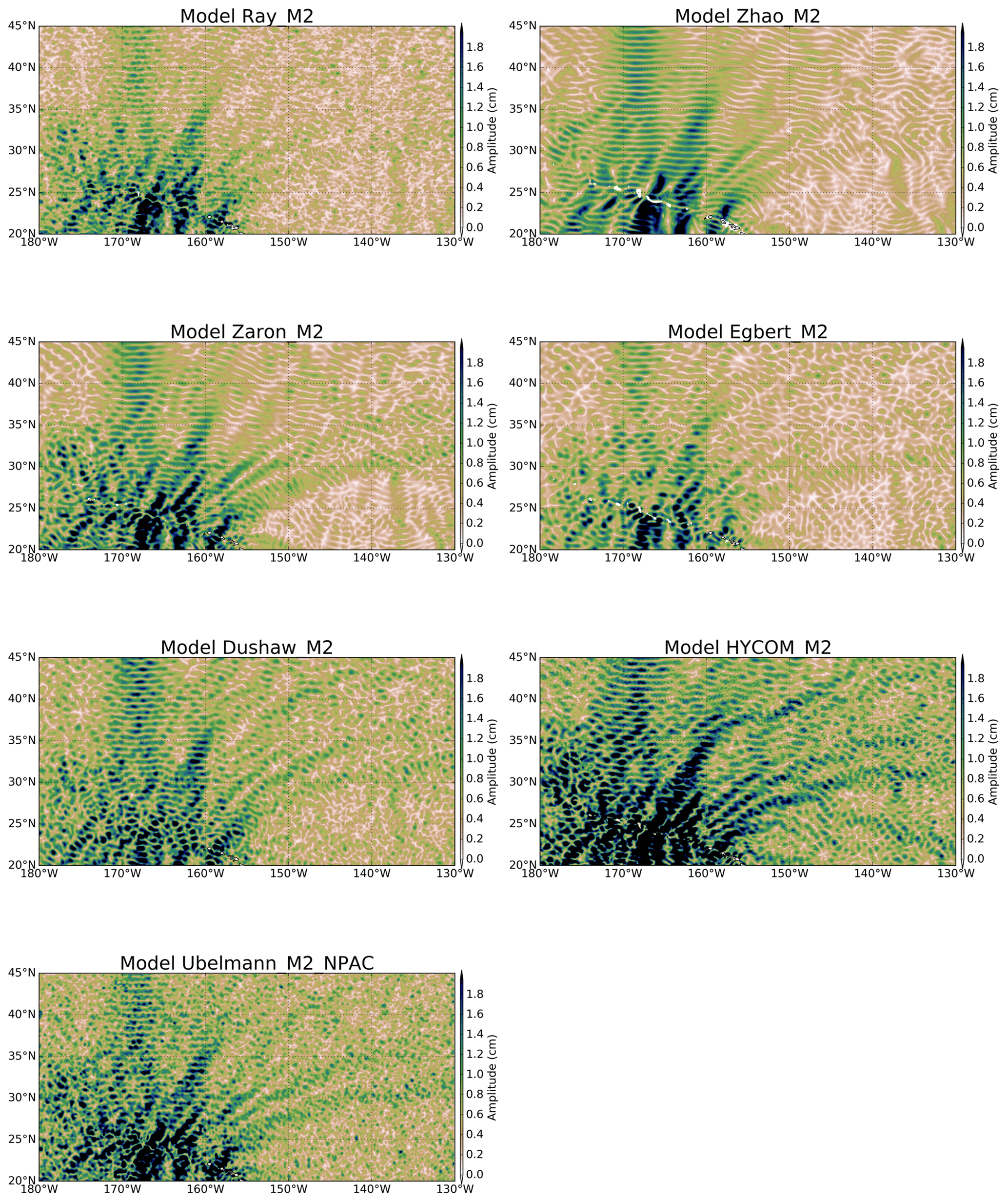
Figure 2Amplitude of the IT models for the M2 tide component in the NPAC region (north Hawaii).
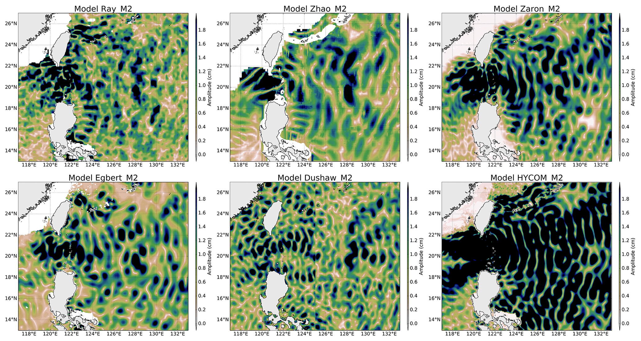
Figure 3Amplitude of the IT models for the M2 tide component in the Luzon area.
Figure 4 shows the amplitude of the three IT solutions available for the K1 wave in the Luzon region, where amplitudes of the diurnal IT are the most important. Models show large-scale (about 200 km or more) patterns on both sides of the Luzon Strait. The K1 scales are greater than the M2 scales as expected from theoretical wavelengths. The K1 amplitude reaches 2 cm on the west side, while patterns and amplitudes of the models differ on the east side of the strait: ZHAO has weaker amplitudes and some different spatial patterns, while ZARON and EGBERT have the solutions that lie closest to one to each other. For these three models, the amplitude of K1 becomes zero at about 24∘ N when getting close to the K1 critical latitude.
Concerning diurnal tides in the global ocean, the ZARON solution is not defined over large regions of the world ocean, including latitudes poleward of the diurnal-tide critical latitude and regions where the IT amplitude is negligible and/or not separable from background ocean variability. The ZHAO solution stops at the diurnal critical latitude, while the EGBERT solution is defined over a wider range of latitudes (until 60∘).
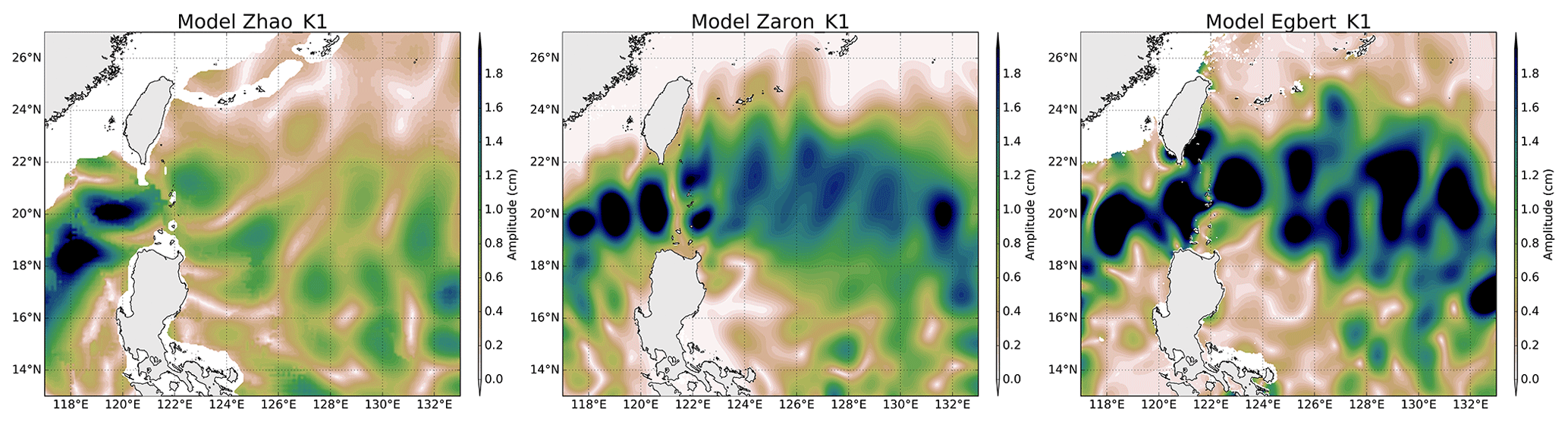
Figure 4Amplitude of the IT models for the K1 tide component, in the Luzon area.
3.2 Quantitative comparison of IT models
Following Stammer et al. (2014), the standard deviation (SD) of all the IT models listed in Table 1 was computed for each tidal constituent with respect to elevation , where ξj is the time-independent amplitude of a tide component at a wet grid point j, σ is tidal frequency and . First, the mean elevation of each tidal constituent across models taken into account (N) is computed at every grid point according to
where with Hj the amplitude and Gj the Greenwich phase lag of the tide considered. Then the SD between all involved models (N) can be computed for each constituent at each grid point according to
where Hn and Gn are the amplitude and the Greenwich phase lag of a constituent given by each model, respectively, and Hmean and Gmean are the mean amplitude and Greenwich phase lag computed from all models from Eq. (1).
The computation of the SDtide was performed for the four tidal constituents M2, S2, K1 and O1, after re-gridding bilinearly the models to a common 1∕20∘ grid. The maps of SD are computed over the global ocean. Note that the DUSHAW model was not included in this SD calculation, as it increases too much the SD value over the global ocean due to noisier patterns in wide regions and makes the results difficult to analyze.
Global maps shown in Figs. 5 and 6 illustrate the mean amplitude and the standard deviation of the M2 and K1 IT models, respectively. Near-coastal regions, shallow-water regions and regions of low signal to noise are masked-out in the maps as they are not defined in most of the studied models. The mean M2 amplitudes reach more than 2 cm in all the known generation sites – in the Pacific, the Indian Ocean around Madagascar, the Indonesian Seas and in the Atlantic offshore of Amazonia. K1 has a significant mean amplitude above 1.5 cm in the Luzon Strait region, in the Philippine Sea and east of Palau and about 0.5–0.7 cm in some regions of the Indian and Pacific oceans.
The map of M2 SD shows small values, generally below 1 cm for M2, indicating good agreement of the IT models in all IT regions defined in Fig. 1 for the M2 wave; the ratio SD ∕ mean amplitude for the M2 wave reaches only 0.2–0.3 around IT generation regions with some clear beam patterns indicating that models agree with each other in those areas. Some larger SD values are found around Luzon Strait, above Madagascar and in the Indonesian seas. For the diurnal wave K1, IT models provide coherent information in the Luzon region, in Tahiti and Hawaii and in the Madagascar region.
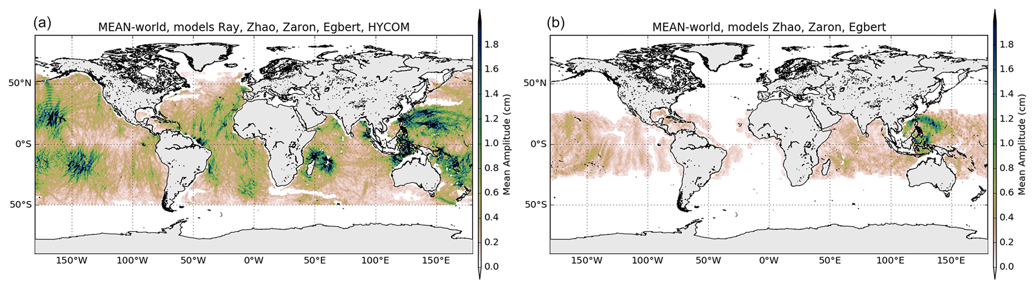
Figure 5Global maps of mean amplitude of the M2 (a) and K1 (b) IT models (cm).
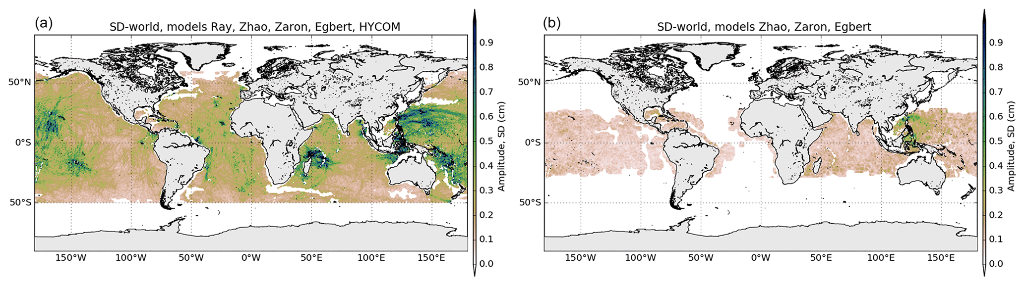
Figure 6Global maps of standard deviation of the M2 (a) and K1 (b) IT models (cm).
The mean standard deviation value is computed over the different regions studied. In order to eliminate any residual barotropic variability likely existing in the empirical IT models in shallow waters, only data located in the deep ocean are used to compute the standard deviation; values are gathered in Table 2. Over all regions, the standard deviation is stronger for M2, consistent with the fact that M2 is the most important IT component in the global ocean. The standard deviation is largest in the Luzon and Madagascar regions, where models give rather different solutions as already seen in the previous section.
The diurnal K1 tide takes on the largest standard deviation value, of 0.25 cm, in the Luzon region, where this diurnal component has the most significant amplitudes.
4.1 The altimeter database
The altimeter measurements used correspond to the level-2 altimeter product L2P, with 1 Hz along-track resolution (LRM), produced and distributed by Aviso+ (https://www.aviso.altimetry.fr/en/data/, last access: 17 December 2020 AVISO), as part of the Ssalto ground processing segment. The version of the products considered is nearly homogeneous with the DT-2014 standards described in Pujol et al. (2016), except for the tide correction as described below.
The altimeter period from 1993 onwards is sampled by 12 altimeter missions available on different ground tracks (https://www.aviso.altimetry.fr/en/missions.html, last access: 17 December 2020). For the purpose of the present study, we use the databases for two different missions:
-
Jason-2 (denoted J2 in the text and figures) is a reference mission flying in the reference TP track with a 10 d cycle and sampling latitudes between ± 66∘; the entire mission time span in the reference track can be used for the study which represents nearly 8 years of data;
-
CryoSat-2 (denoted C2 hereafter) is characterized by a drifting polar orbit sampling all polar seas and it has a nearly repetitive sub-cycle of about 29 d.
The mission's time series and the number of cycles used for the present study are listed in Table 3. It is worth pointing out that much of the T/P and Jason data have been used in most of the IT empirical solutions tested (see Table 1), but all models are independent of CryoSat-2 mission data.
Due to sub-optimal time sampling, altimeters alias the tidal signal to much longer periods than the actual tidal period. The aliased frequencies of the four main tidal waves studied are listed in Table 3 for the two orbits used. It is noticeable that the diurnal tide K1 is the most difficult to observe with satellite altimetry as it is aliased to the semiannual period by the J2 orbit and to a nearly 4-year period by the C2 satellite orbits. C2 aliasing periods are very long compared to Jason's ones.
Table 2Spatial-mean SD (cm) of the M2 and K1 IT models for each studied region.
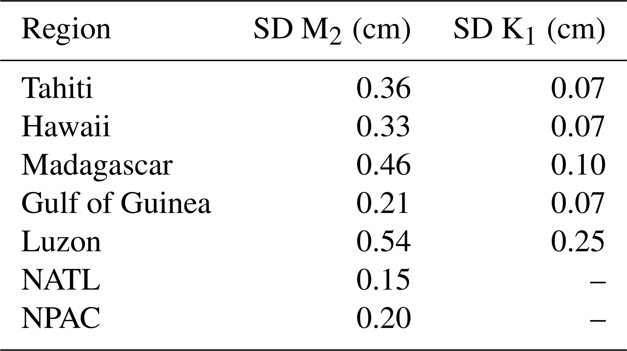
Table 3Description of the altimeter database for the validation study, along with the associated aliasing periods for the main tidal components.
The altimeter sea surface height (SSH) is defined as the difference between orbit and range, corrected from several instrumental and geophysical corrections as expressed below:
where
-
tide includes the geocentric barotropic tide, the solid Earth tide and the pole tide corrections. The geocentric barotropic tide correction was updated compared to the altimetry standards listed in Pujol et al. (2016) and comes from the FES2014b tidal model (https://www.aviso.altimetry.fr/en/data/, last access: 17 December 2020; Carrere et al., 2016a; Lyard et al., 2020);
-
IT is the internal-tide correction, taken one by one from each model studied in this paper;
-
other_corr includes the dynamic atmospheric correction, the wet tropospheric correction, the dry tropospheric correction, the ionospheric correction, the sea state bias correction and complementary instrumental corrections when needed, as described in Pujol et al. (2016).
The sea level anomaly (SLA) is defined by the difference between the SSH and a mean profile (MP) for repetitive orbits or a mean sea surface (MSS) for drifting orbits. Mean profiles computed for TOPEX or the Jason orbit for the reference period of 20 years (1993–2012), have been used within the present study for the J2 mission (Pujol et al., 2016), and the MSS_CNES_CLS_11 also referenced on the same 20 years period was used for the C2 drifting orbit mission (https://www.aviso.altimetry.fr/en/data/products/auxiliary-products/mss.html, last access: 17 December 2020; Schaeffer et al., 2012; Pujol et al., 2016; Appendix A).
4.2 Method of comparison
Satellite altimetry databases can be used to evaluate many geophysical corrections and particularly global barotropic tidal models as already examined by other authors (Stammer et al., 2014; Carrere et al., 2016a, b; Lyard et al., 2006; Carrere, 2003). We propose using a similar approach to validate the concurrent IT models listed in Table 1.
First, we generate the corresponding IT correction for each along-track altimeter measurement, computed from the interpolation of each IT atlas onto the satellites' ground tracks and the use of a tidal prediction algorithm. Each tidal component is considered separately for the clarity of the analysis, keeping in mind that the various IT models do not all contain the same waves.
Second, the altimeter SSH using IT corrections from each model tested can then be computed, and the differences in the sea level contents are analyzed for different time and spatial scales. In particular, considering several altimeters allows the study of different temporal periods. As the missions considered, J2 and C2, have different ground tracks and different orbit (cycle) characteristics, several aliasing characteristics are tested.
Third, the impact of each IT model on SSH can be estimated for short temporal scales (time lags lower than 10 d), which are the main concern here as we consider the main high-frequency tidal components M2, K1, O1 and S2. Moreover, these short temporal scales also impact climate studies since high temporal-frequency errors increase the formal estimation error of long-timescale signals (Ablain et al., 2016; Carrere et al., 2016b). The impact of using each of the studied corrections on the SSH performances is estimated by computing the SSH differences between ascending and descending tracks at crossovers of each altimeter. Crossover points with time lags shorter than 10 d within one cycle are selected in order to minimize the contribution of the ocean variability at each crossover location. For the purpose here, we avoid all strong assumptions about internal tide and assume coherent internal tides have short autocorrelation scales.
Fourth, the variance of SSH differences at crossover points is computed on boxes of 4∘ × 4∘ holding all measurements within the time span of the mission considered according to
where ΔSSHITzero is the SSH differences at crossovers using a zero IT correction within a 4∘ × 4∘ box for the period considered and ΔSSHITi is the SSH differences at crossovers using one of the IT models listed in Table 1 within the same box and period. The resulting maps give information on the spatiotemporal variance of the SSH differences within each box. As SSH differences are considered, this variance estimation is twice the variance difference of SLA. A reduction in this diagnostic indicates an internal consistency of sea level between ascending and descending passes within a 10 d window and thus characterizes a more accurate estimate of SSH for high frequencies. However, the spatial resolution of this diagnostic is limited due to the localization of crossovers and the 4∘ resolution of the grid. Particularly for C2, the mission ground tracks' pattern induces a non-homogeneous spread of crossovers over the global ocean, with no crossovers around latitudes 0∘ and ± 50∘. For J2, all latitudes are covered with crossovers but the number of points is not homogeneous over the ocean: it is limited at the Equator and increases towards the poles.
Fifth, along-track SLA statistics can be calculated from 1 Hz altimetric measurements and allow for a higher spatial resolution in the analysis. The maps of the variance difference of SLA using either the IT correction tested or the reference ZERO correction are computed on boxes of 2∘ × 2∘ according to
where SLAITi (or SLAITzero) are the SLA computed using one of the IT corrections listed in Table 1 (or using the zero IT correction) in the period considered and within one 2∘ × 2∘ box. Although high-frequency signals are aliased in the lower-frequency band following the application of the Nyquist theory to each altimeter sampling, SLA time series contain the entire ocean variability spectrum. The SLA variance reduction diagnostic shows an improvement of the studied IT correction, on the condition that the correction is decorrelated from the sea level.
Sixth, the mean of these variance reduction estimations at crossovers and for along-track SLA is computed for each studied region, which allows an easier analysis and comparison of the performances of the IT model tested.
Finally, in order to quantify the impact of each IT model on the SLA variance reduction in terms of spatial scales, a spectral analysis of J2 SLA is performed in the different regions of interest, and details are given in Sect. 6.
This section gathers the validation results of each IT model using the satellite altimetry databases described previously. For the clarity of the analysis, each IT correction is compared to a reference correction using a ZERO correction. For the ZERO correction, no IT correction is applied, as in the actual altimeter geophysical data records version-D and version-E (GDR-D and GDR-E) processing (Pujol et al., 2016; Taburet et al., 2019). The complete diagnostics and analysis are presented hereafter for the largest semidiurnal (M2) and diurnal (K1) components; results for the second-largest semidiurnal (S2) and diurnal (O1) IT are gathered in the Appendix of the paper.
5.1 M2 component
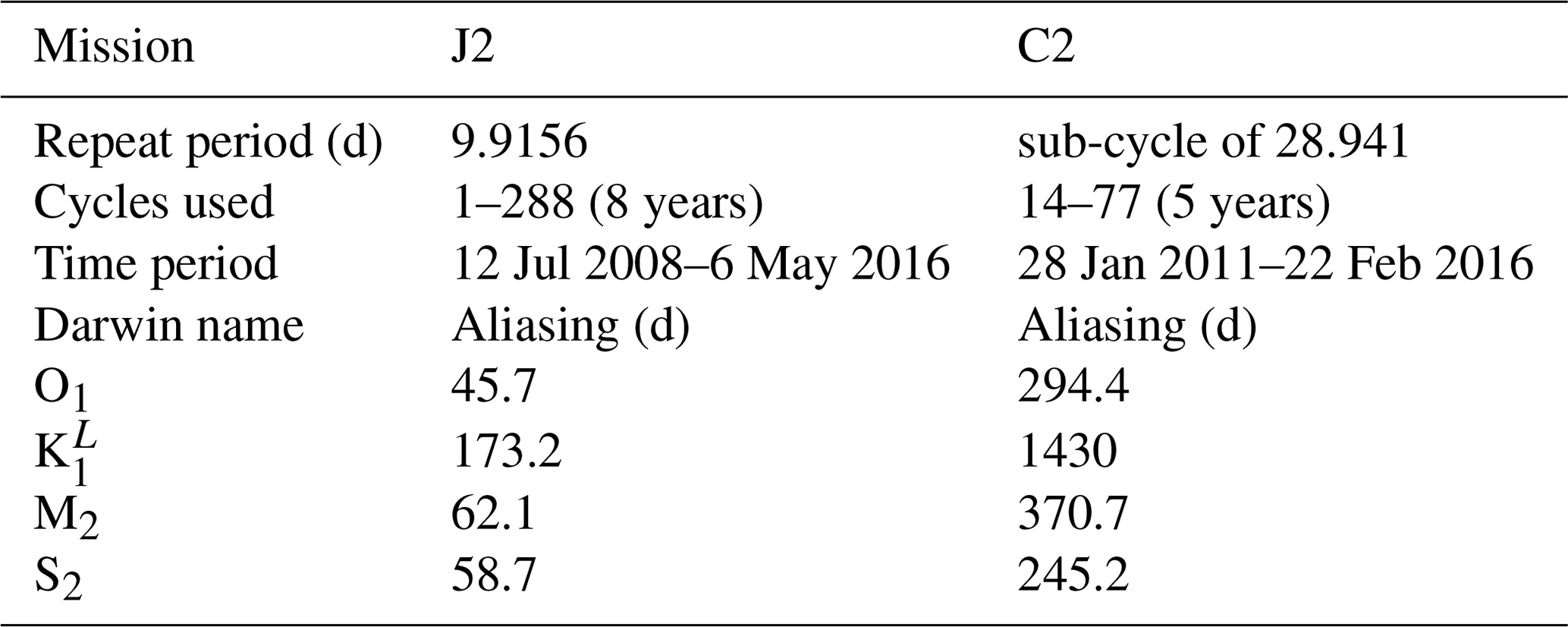
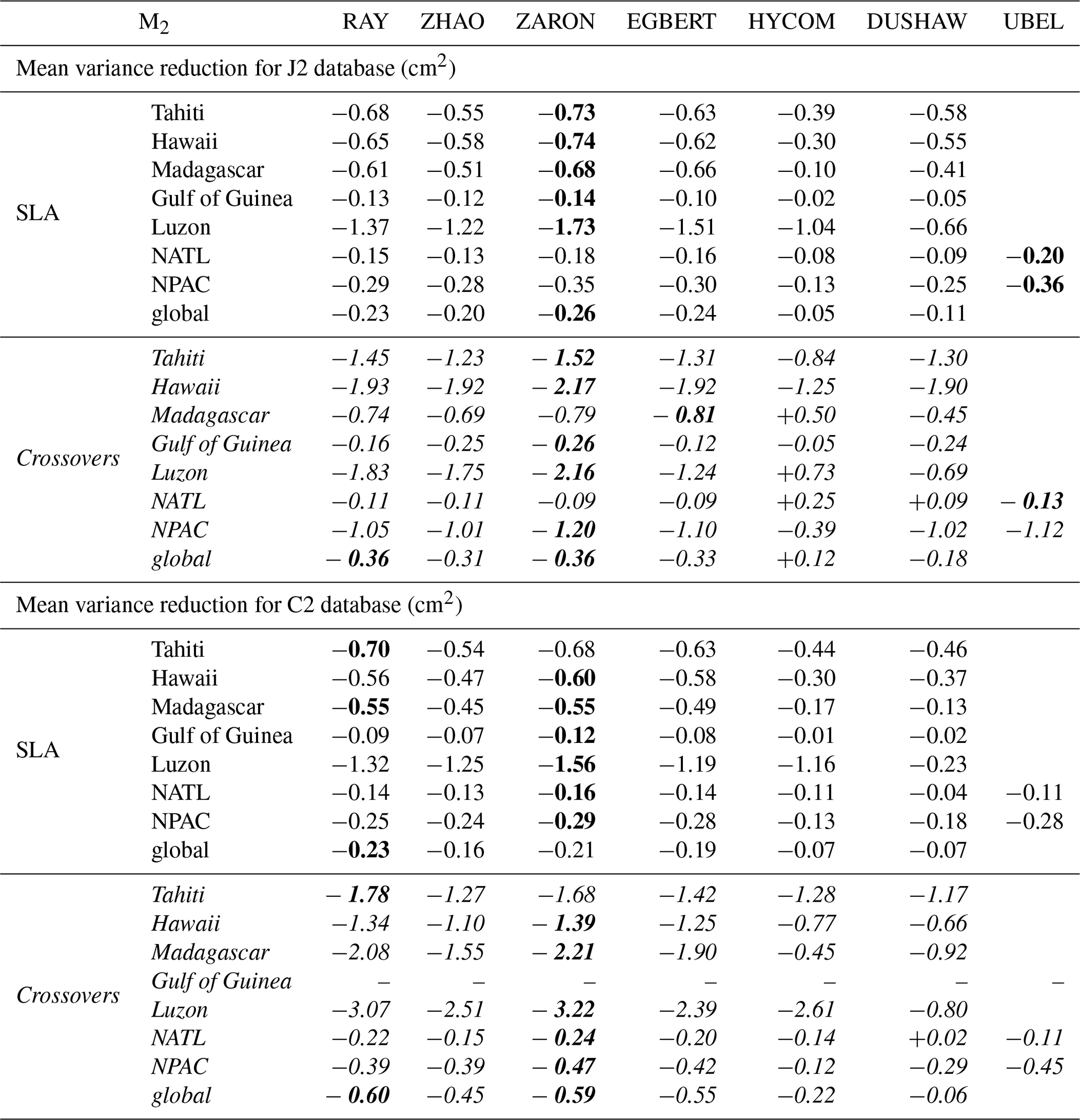
To investigate and quantify the regional impact of the M2 IT corrections, the maps of SSH variance difference at crossovers using either IT correction from each model or a ZERO reference correction, are plotted for the J2 mission in Fig. 7. Note that the quantification and the regional analysis of the M2 IT correction can be performed for the seven IT models participating in the present study. Most of the IT models reduce the altimeter SSH variance in all IT regions. The RAY and ZARON models are the most efficient, with a variance reduction reaching more than 5 cm2 in many areas. The HYCOM and DUSHAW models reduce SSH variance in some locations but also raise the variance locally: mostly in large deep ocean regions where IT signal can be weak in other models for HYCOM, while the DUSHAW model raises variance mostly in areas of strong currents. Mean values, averaged over the strong IT regions shown in Fig. 1, are listed in Table 4: the more energetic areas for the M2 IT seem to be the Luzon Strait and Hawaii regions with a mean SSH variance reduction greater than 2 cm2 for the ZARON model. The ZARON model is the most efficient in all areas except in the North Atlantic (NATL) region where the UBELMANN model reduces slightly more variance. Over the global ocean, the EGBERT, ZARON, ZHAO and RAY models have similar mean performances, but RAY reduces a bit more the J2 variance globally (0.34 cm2).
Figure 8 displays the maps of along-track J2 SLA variance differences using the M2 IT correction from each model and a ZERO reference correction. Spatial patterns are similar to those in Fig. 7. However, using the along-track SLA allows for a better spatial resolution in the output variance maps. In addition, regions of strong IT and regions of strong ocean currents are more clearly identified. The DUSHAW model raises SLA variance in several mesoscale regions (Gulf Stream, Agulhas current, Argentine basin and Kuroshio currents), likely indicating that the model does not properly separate IT and other oceanic signals in these strong-current areas; the ZHAO model also raises the variance in those regions slightly, while EGBERT reduces the SLA variance in the Gulf Stream and Agulhas regions. HYCOM raises the variance over wider regions in the three oceans than the empirical and assimilative models do: this is likely due to its intrinsic characteristic of the free hydrodynamic model which may induce more phase errors compared to constrained or empirical models and also due to the short HYCOM time series duration used to extract the IT atlas, which induces stronger IT amplitudes (see Ansong et al., 2015; Buijsman et al., 2020). These maps also indicate that the four models RAY, EGBERT, ZARON and ZHAO, reduce the SLA variance in some additional IT areas which are not specifically investigated in the present study: the Indonesia seas and south of Java, north of Sumatra, between the Solomon Islands and New Zealand in Pacific, off the Amazonian shelf, and in many regions of the Atlantic Ocean. Mean values, averaged over the strong IT regions identified in Fig. 1, are given in Table 4: mean J2 SLA variance reductions are weaker than the crossover difference variances by construction, but they indicate similar conclusions as for J2 crossover differences: the ZARON model is the most efficient to reduce the SLA variance in all IT regions, except in NPAC and NATL, where the UBELMANN model is slightly more efficient. Mean values over the global ocean are close for the four models EGBERT, ZHAO, ZARON and RAY, with the two last ones showing a slightly better performance than others.
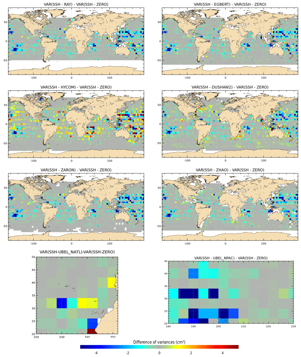
Figure 7Maps of SSH variance differences at crossovers using either the M2 IT correction from each model or a ZERO reference correction in the SSH calculation for the J2 mission (cm2). J2 cycles 1–288 have been used.
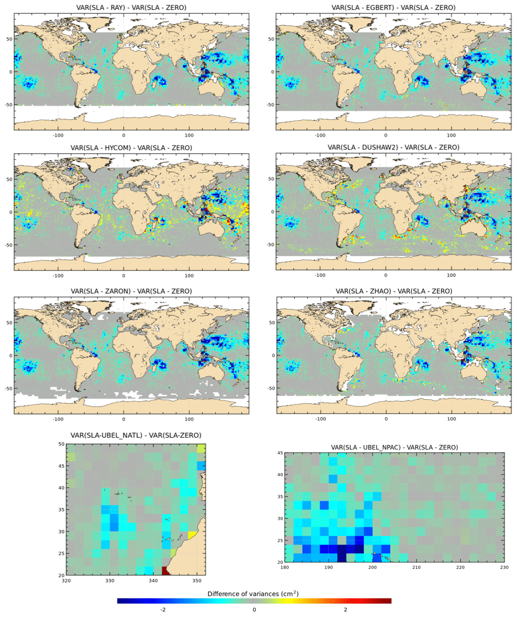
Figure 8Maps of SLA variance differences using either the M2 IT correction from each model or a ZERO reference correction in the SLA calculation for the J2 mission (cm2). J2 cycles 1–288 have been used.
One should note that those J2 results might be biased in favor of the empirical models, as J2 data are used in all of them except for the DUSHAW model (see Table 1). To check these results, similar diagnostics are computed using the C2 altimeter database, as described in Sect. 4.1, which is an independent database for all models. Validation results are given in Figs. 9 and 10 for C2 SSH crossover differences and C2 SLA, respectively.
Validations with the C2 database show similar results as for J2, with a significant variance reduction in the C2 SSH differences and SLA for most models in all IT regions; variance gain patterns are generally similar but more widely spread and stronger in C2 SSH maps compared to J2 particularly in the Atlantic Ocean and in the west Pacific. The pattern is different for the UBELMANN model in the NATL region, likely due to some inclusion of J2 errors or signal or larger-scale signals in the model (see Sect. 6). The ground track pattern of the C2 orbit explains the lack of crossover data at 0∘ and ± 50∘ latitudes bands. C2 SLA variance maps have similar patterns compared to J2, and some additional IT regions are pointed out, which corroborates the quality of the different IT models tested. Over both C2 SSH and SLA, the HYCOM and DUSHAW models show a significant addition of variance in some regions, similarly as for J2 results.
Figure 9Maps of SSH variance differences at crossovers using either the M2 IT correction from each model or a ZERO reference correction in the SSH calculation for the C2 mission (cm2). C2 cycles 14–77 have been used.
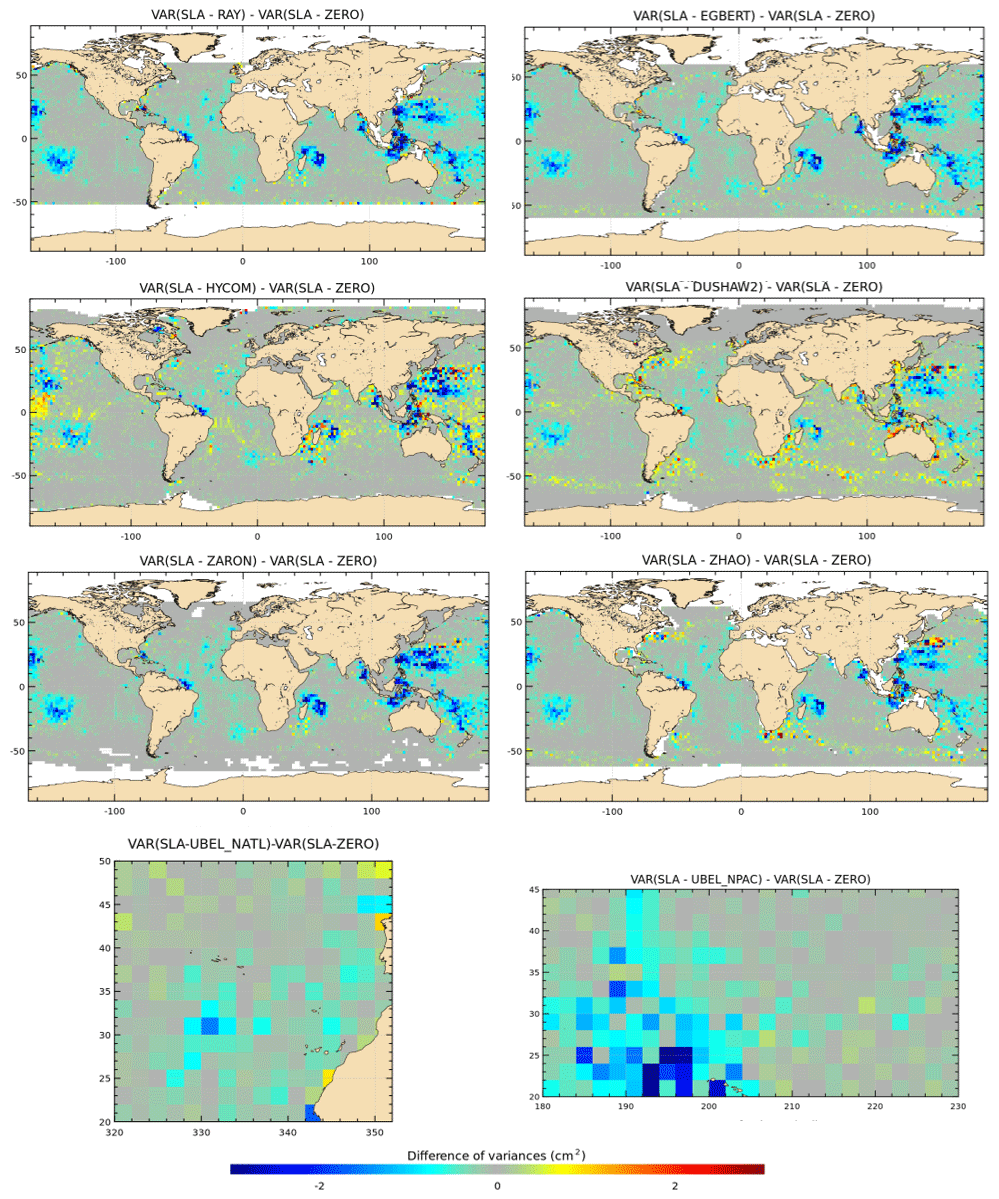
Figure 10Maps of SLA variance differences using either the M2 IT correction from each model or a ZERO reference correction in the SLA calculation for the C2 mission (cm2). C2 cycles 14–77 have been used.
Mean values for C2 data, averaged over the strong IT regions, are also given in Table 4. Mean C2 SLA variance gains are comparable to J2 mission on all IT regions. C2 validation results for the M2 IT component show that the ZARON model performs better than other models in most IT regions studied, with a maximum reduction in SSH difference variance of 3.2 cm2 in Luzon and 2.2 cm2 in the Madagascar area. RAY reduces variance a bit more in the Tahiti region; on average over the global ocean, the ZARON and RAY models are the most efficient.
Table 4Mean variance reduction for the J2 and C2 altimeter databases, within each IT region, when using the different M2 internal-tide models and compared to the ZERO correction case; variance reduction in altimeter SLA (white lines) and for altimeters crossover differences (italic lines) for each mission, in square centimeters. For each IT region, the maximum variance reduction across the different models is in bold.
5.2 K1 component
The maps of K1 SSH variance difference at crossovers using the K1 IT correction from EGBERT, ZARON and ZHAO models are plotted in Fig. 11 for the J2 and C2 missions. Note that unlike the M2 wave analysis, the quantification and the regional analysis of the K1 IT correction can be performed for only three IT models participating in the present study that provide a K1 solution, as the diurnal tides are more difficult to detect and sort out by altimetry. The K1 IT solutions are compared to a ZERO reference correction. The three models have different approaches to take into account the diurnal tides' critical latitude and regions where amplitude of K1 IT is negligible and/or not separable from background ocean variability (cf Sects. 2 and 3.1), which explains the large non-defined regions in ZARON and ZHAO maps compared to EGBERT. Results show that the three IT models all reduce the J2 SSH variance strongly in the west Pacific or Luzon and Indonesian regions (more than 2 cm2), while a weaker variance reduction is visible in the central Indian and central Pacific areas (0.5–1 cm2). The reduction is also important for C2 SSH in the east Pacific or Luzon area and south of Java, and results are noisier in the other oceans where diurnal IT is weak, but C2 data are likely less efficient for testing the K1 tide due its very long alias compared to M2 tide (see Table 3). The ZARON model reduces slightly more C2 variance in the southern part of the Indian Ocean.
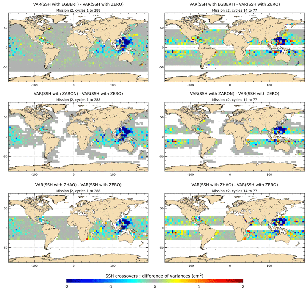
Figure 11Maps of SSH variance differences at crossovers using either the K1 IT correction from each model or a reference ZERO correction in the SSH calculation for the J2 and C2 missions (cm2). J2 cycles 1–288 have been used; C2 cycles 14–77 have been used.
The maps of SLA variance differences using the EGBERT, ZARON and ZHAO K1 IT models are plotted in Fig. 12 for the J2 and C2 missions. Spatial SLA patterns are consistent with the SSH maps of Fig. 11 and allow a better spatial resolution compared to SSH maps as also noted for M2 results: using the EGBERT model allows a significant reduction in the J2 SLA variance mostly in the Luzon Strait or west Pacific region and the northern Indonesian seas, where the amplitude of the K1 IT is the most important; a weak variance gain is also visible in the IT regions around Tahiti, Hawaii and north of Madagascar but also in some large ocean current regions, in the central Indian Ocean and east of Australia. The other maps indicate that ZHAO is less efficient than the two others in the Luzon region, while ZARON reduces slightly more variance for the C2 mission in the west Pacific area.
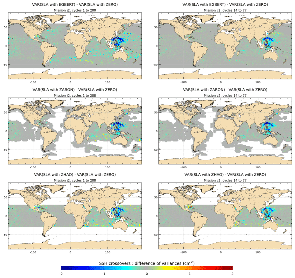
Figure 12Maps of SLA variance differences using either the K1 IT correction from each model or a reference ZERO correction in the SLA calculation for the J2 and C2 missions (cm2). J2 cycles 1–288 have been used; C2 cycles 14–77 have been used.
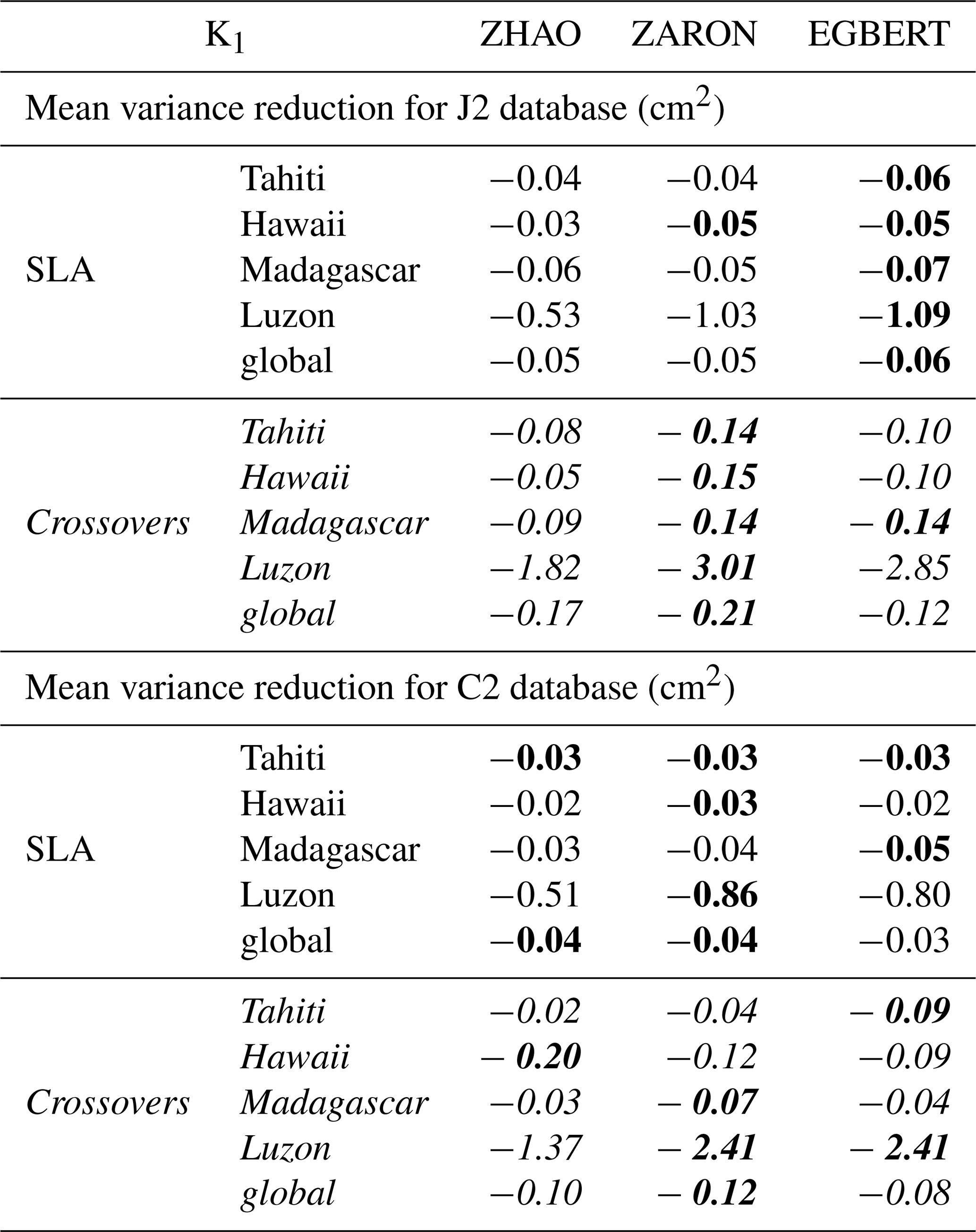
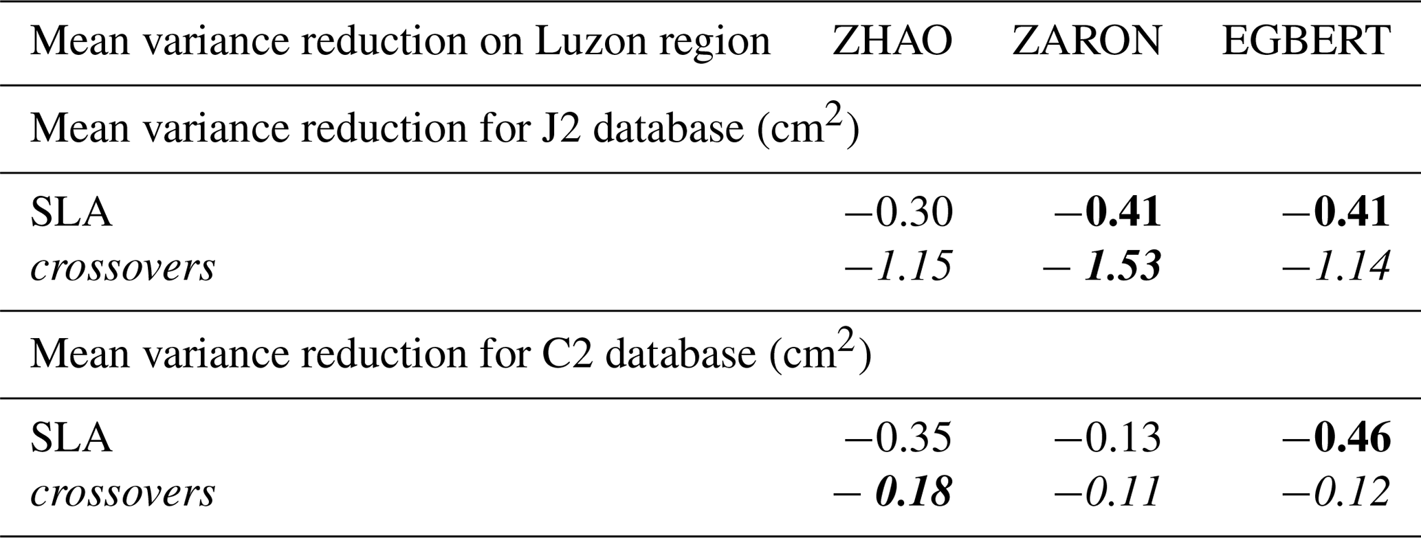
The mean statistics of altimeter variance reduction, over the regions defined in Fig. 1, are given in Table 5 for the SLA and the SSH differences of J2 and C2 missions and for the different regions studied; note that we focus on Luzon, Tahiti, Hawaii, Madagascar and global areas because mean K1 statistics are not significant in the other regions of large semidiurnal tides defined in Fig. 1. The values in Table 5 indicate a significant variance reduction mainly in the Luzon region as expected from the analysis of global maps. The ZARON and EGBERT models are the most efficient IT solutions in the Luzon region, with similar variance gains for both models at C2 crossovers. ZARON shows a significant variance gain compared to the ZERO correction for both missions tested, reaching 3 and 2.4 cm2, respectively, for J2 crossovers and C2 crossovers.
Table 5Mean variance reduction for J2 and C2 altimeter databases, within each IT region, when using the different K1 internal-tide models and compared to the ZERO correction case; variance reduction in altimeter SLA (white lines) and for altimeter crossover differences (italic lines) for each mission, in square centimeters. For each IT region, the maximum variance reduction across the different models is highlighted in bold.
In order to quantify the impact of each IT model on the altimeter SLA variance reduction as a function of spatial scales, a spectral analysis of J2 along-track SLA is performed. This analysis is not conducted for other missions because the duration of the C2 mission time series used is too short to allow a proper spectral estimation at the aliasing frequency of M2 (cycle duration is 370 d for C2). Moreover, this diagnostic only focuses on the main M2 IT because the K1 aliasing frequency by J2 sampling is 173 d (see Table 2), which makes it barely separable from the semiannual ocean signal.
The J2 SLA spectral analysis is performed for each of the IT regions described in Fig. 1. For each area, a frequency–wavenumber spectrum is computed for the along-track SLA and for the SLA corrected from each IT solution; the spectral density at a 62 d frequency, which is the aliasing frequency band of the M2 tidal component by Jason's orbit, is extracted in both cases and then the normalized difference of the spectral density is computed and plotted as a function of wavelength. This computation gives an estimation of the percentage of energy removed at the M2 frequency thanks to each IT model correction, as a function of wavelength and for the different regions studied.
Results for the different regions are gathered in Fig. 13 and show that all empirical models generally manage to remove an important amount of coherent IT energy for the first mode (wavelengths of about 150 km): the reduction in energy reaches about 50 %–80 % depending on the area. Some empirical models also perform well for shorter scales. The DUSHAW model is generally less efficient in the different regions except in the Gulf of Guinea where it is as efficient as others for the first mode. In the Tahiti, Luzon, Gulf of Guinea and NATL regions, ZARON is the most efficient model with a very significant reduction in the energy for the first and the second IT modes: the ZARON model removes 80 % of the energy at the M2 frequency for the first internal-tide mode and 70 % for the second mode in the Tahiti region. With respect to the first mode, the ZARON model removes nearly 80 % of the energy in the Gulf of Guinea, 60 % in the Luzon, Madagascar and NPAC regions, and 50 % in the NATL region. We speculate that the regions for which ZARON removes less variance may be regions with stronger IT non-stationarity (Zaron, 2017). In the Madagascar region, ZARON, EGBERT, RAY and ZHAO perform similarly for the first mode. Only a few models manage to reduce the IT energy for the second and the third modes: RAY and ZARON reduce more than 60 % of the second mode energy around Tahiti and up to 30 % in other regions except in NATL where they only reduce about 15 % of the second mode energy. Aside from the fact that models are not perfect, these results corroborate the fact that the non-stationary IT part is even more significant for higher IT modes (Shriver et al., 2014; Rainville and Pinkel, 2006). Around Tahiti, the curves indicate that the RAY model also reduces the SLA energy for a third mode of IT (∼ 20 %). The ZHAO model also removes some energy at short scales in the Madagascar and Luzon regions.

Figure 13Normalized difference of the power spectral density of J2 SLA as a function of wavelength and for each IT region studied. Blue line – DUSHAW model; green – EGBERT model; red – HYCOM model; light blue – RAY model; purple – ZARON model; light green – ZHAO model; black – UBELMANN model.
The black curves show the performances of the UBELMANN model in the NATL and NPAC regions: it is very efficient in NPAC with a similar energy reduction as the ZARON model for the first and second modes, and it also removes some signal at shorter scales. In the NATL area, the UBELMANN model seems to be more efficient than all other models for all wavelengths and also for large scales, which likely indicates that the model also includes some large-scale signals which are not internal tides but rather some residual barotropic tide signals or even some non-tidal ocean signal aliasing.
The assimilative model, EGBERT, has performances comparable to the purely empirical models for the first mode, but it does not have enough energy for the shorter IT modes except for two regions: for the Madagascar region the EGBERT model reduces the SLA energy for scales of 60–70 km, and for the Gulf of Guinea region it reduces energy in shorter modes compared to other models (scales shorter than 60 km).
It is also interesting to point out that the pure hydrodynamic model, HYCOM, removes energy for the three first IT modes in some of the regions studied: although weaker than for the empirical models, the HYCOM gain reaches 55 % for the first mode, 40 % for the second mode and 15 % for the third mode in the Tahiti area. The gain is weak but noticeable in the NATL, NPAC, Luzon and Madagascar regions, but the local rise of energy in some regions also indicates that the hydrodynamic model still has some uncertainties, particularly in the Gulf of Guinea region and for short IT scales in the Madagascar region.
Seven models of the coherent IT surface signature have been extensively compared within the present study: Dushaw (2015), Egbert and Erofeeva (2014), Ray and Zaron (2016), Shriver et al. (2014), Clément Ubelmann, personal communication, Zaron (2019), and Zhao et al. (2016). They are of three types: empirical models based upon analysis of existing altimeter missions, an assimilative model and a three-dimensional hydrodynamic model.
Recently updated Jason-2 and CryoSat-2 altimeter databases have been used to validate these new models of coherent internal tides over the global ocean, focusing on the four main IT frequencies: M2, K1, O1 and S2. First, the analysis shows clearly the value of using such a complete altimeter database to validate IT models. The great quality of the database allows the investigation of small-amplitude signals over the entire ocean, and the different sampling characteristics of the various missions complement each other well. The results point to a significant altimeter variance reduction when using the new IT correction models over all ocean regions where internal tides are generated and propagating. Moreover, the spectral approach quantifies the efficiency of the variance reduction potential of each model as a function of horizontal wavelengths – the latter is particularly valuable information for the SWOT mission, which will focus as never before on short wavelength phenomena.
All empirical models display generally good performance for M2, K1, O1 and S2, but the DUSHAW solution performs slightly less well. The ZARON and RAY models have similar results for the first three IT modes, but the ZARON model removes more variability than all other models over most of the strong IT regions analyzed. It is also noticeable that some models (DUSHAW and ZHAO) still remove some variability in areas of strong currents, likely due to some residual leakage of the mesoscale variability. The UBELMANN solution appears to also remove some large-scale, likely residual barotropic tide signal in the northeast of the Azores area.
The assimilative model (EGBERT) has performances comparable to the empirical models, but it also removes some variability in regions of strong currents, likely due to some remaining mesoscale variability in the assimilated data.
The hydrodynamic solution, computed from a HYCOM simulation, is also able to reduce some of the internal-tide variability in most of the IT regions studied, which is a very encouraging result. However, the analysis indicates that it is not yet mature enough to be compared to empirical models. The HYCOM solution has stronger amplitudes compared to the other models, which is likely due to the effects of the relatively short HYCOM time series duration (1 year) on the IT estimation (see Ansong et al., 2015). Indeed, some tests showed that using a reduction coefficient (Buijsman et al., 2020) that accounts for the short duration of the time series used in the analysis slightly improves the performance of the HYCOM hydrodynamic solution. Ongoing work is testing whether operational HYCOM simulations, which assimilate altimeter measurements of mesoscale eddies and improve the underlying stratification relative to observations (e.g., Luecke et al., 2017), will yield improvements in the skill of the predicted internal tides in HYCOM.
The results described here and for which we provide a scientific justification, have been also presented at the last OSTST (Ocean Surface Topography Science Team) meetings of Ponta Delgada Miguel (2018; program available at https://meetings.aviso.altimetry.fr/programs/2018-ostst-complete-program.html, last access: 18 January 2021) and Chicago (2019; program available at https://meetings.aviso.altimetry.fr/programs/2019-ostst-complete-program.html, last access: 18 January 2021): in the light of these findings, the recommendation came to use an internal-tide model for the correction of all along-track nadir altimeter databases as well as the upcoming high-resolution SWOT wide-swath altimeter mission. Consequently, the ZARON model is being implemented in the next version of the altimeter GDRs (GDR-F-standard: https://www.aviso.altimetry.fr/en/data/, last access: 17 December 2020), which will be available on AVISO.
In addition, the impact of using the ZARON IT correction has also been estimated for the level-4 (L4) altimeter products, which are global gridded data. A significant improvement was detected in all the regions of interest, and it was demonstrated that this new correction reduces the remaining IT signal in the L4 AVISO/CMEMS (Copernicus Marine Environment Monitoring Service) products (Faugère et al., 2019; Zaron and Ray, 2018). Accordingly, this IT correction will be used to compute the SLA for the next Duacs reprocessing product Duacs-2021, which is currently being undertaken. Moreover, the implementation of this new IT correction is planned in the future CMEMS L3 and L4 altimeter product version coming in 2021.
The present study indicates that the use of the altimetry database is a valuable tool to validate models of IT surface signature in the global ocean. It particularly complements the in situ validation processes which are generally more localized in space or time due to the availability of in situ datasets (Dushaw et al., 1995, 2017; Dushaw, 2006, 2015; Zaron and Ray, 2018).
Within the SWOT mission preparation, several teams pursue ongoing efforts concerning the better understanding and modeling of IT in the global ocean, and the work presented here could help validate the new model solutions produced. The perspectives of improvement of IT models concern the coherent internal tides through the inclusion of higher IT modes and more tidal frequencies. Many initiatives are also being conducted to try to better understand and model the non-stationary component of the internal tides. Work is progressing on the modeling of the seasonal and interannual internal-tide variability: Zhao (2019b), Zaron (2019), Richard D. Ray (personal communication, 2019) and Clément Ubelmann (personal communication, 2020). And within the SWOT Science Team and other projects, several teams are also working on 3D simulations using different general circulation models such as HYCOM, MITgcm, NEMO (CMEMS–Mercator–Ocean, project in progress) or even a specific spectral approach (Barbot et al., 2020).
Amplitudes of O1 and S2 tide components for each IT model are plotted in Figs. A1 and A2, respectively, in the Luzon area. Concerning the O1 tide, ZHAO and ZARON show a similar south-west pattern on the west side of the Luzon Strait, with an amplitude reaching more than 2 cm for ZARON and only the half for ZHAO's solution. On the east side of the strait, the three models are quite different: ZHAO has the weaker amplitudes, ZARON has strong large-scale patterns propagating far eastward (1.5 cm amplitude with 200 km wide features) and decaying to zero above 22∘ N; and EGBERT shows a third very different pattern with zero amplitude along latitudes 15 and 21∘ N and also east of the Philippines and amplitudes reaching about 1 cm at 22–23∘ N.
In this region, the S2 IT amplitude shows smaller spatial scales than O1 and close to the M2 ones as expected. The EGBERT S2 solution is very different from others and mostly shows a noisy pattern in this Luzon area. ZHAO and ZARON show similar features of about 1 cm amplitude and with a clear eastward propagation in the Pacific Ocean and a northwestward direction west of the strait; ZARON has stronger amplitudes.
Global maps shown in Figs. A3 and A4 illustrate the mean IT amplitude and the standard deviation of the IT models for the O1 and S2 tidal component, respectively. S2 mean amplitudes show similar patterns as M2 with weaker amplitudes as expected (below 1 cm); the main S2 generation sites are visible around Hawaii in the Pacific Ocean, off Amazonia, around Madagascar, north of Sumatra, south of Lombok, in the Banda and Celeb seas, around the Solomon Islands, in the Luzon area, and on the Saipan ridge. O1 IT has similar patterns as K1 but with weaker mean amplitudes.
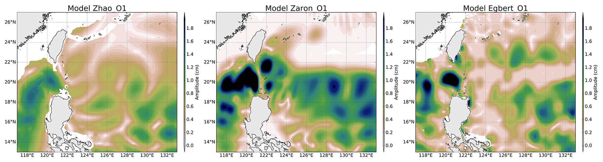
Figure A1Amplitude of the IT models for the O1 tide component in the Luzon area.
Table A1Spatial-mean SD of models for S2 and O1 tide components for each studied region (in centimeters).
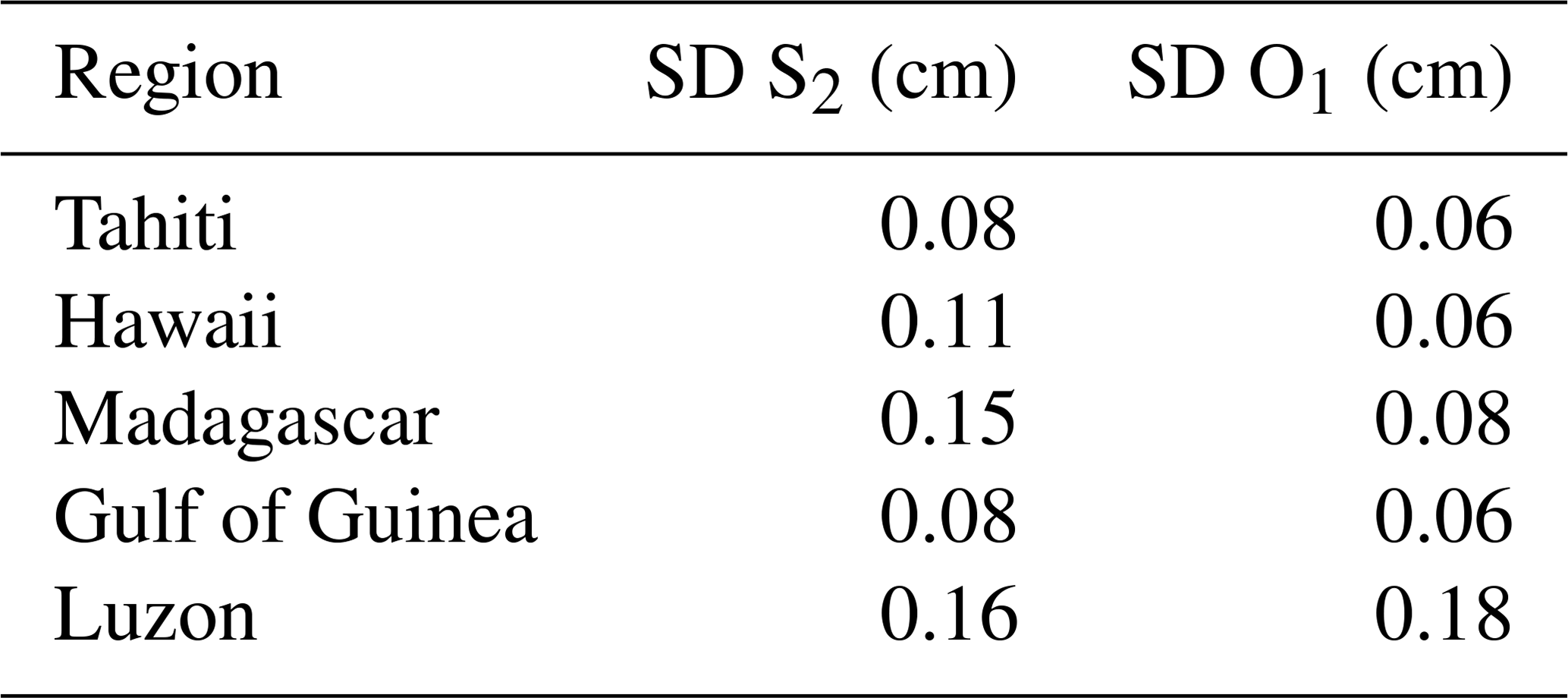
For O1, the Luzon Strait region mainly stands out with stronger standard deviation values in the Luzon Strait and eastwards in the Philippine Sea (values around 0.4 cm). The S2 standard deviation reaches 0.1–0.5 cm in the Hawaii, Madagascar and Luzon regions, where the amplitude of the S2 IT signal is more important. The mean standard deviation is computed in the different regions studied, using only data located in the deep ocean, and values are gathered in Table A1. The S2 mean standard deviation is at least 3 times smaller compared to M2, which is coherent with the fact that S2 IT has a smaller amplitude than M2; stronger values occur in the Luzon and Madagascar regions, where mean S2 IT amplitude is maximal. O1 IT has the strongest standard deviation (0.18 cm) in the same Luzon area as K1, where diurnal internal tides have the most significant amplitudes in the ocean, which indicates that O1 IT models have some uncertainties in this region.
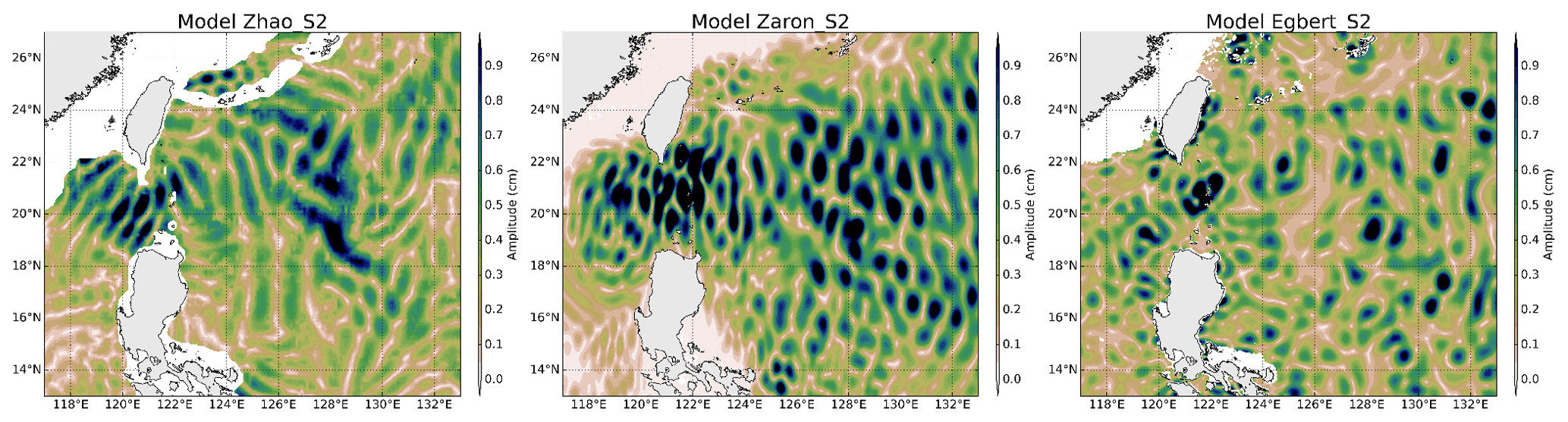
Figure A2Amplitude of the IT models for the S2 tide component in the Luzon area.

Figure A3Global maps of mean amplitude of the O1 (a) and S2 (b) IT models (cm).
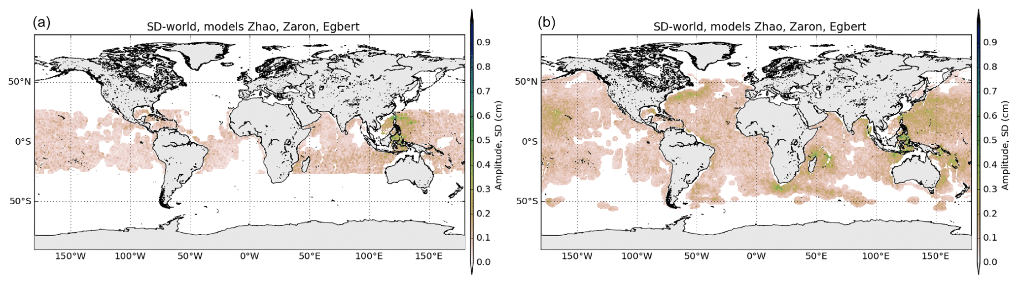
Figure A4Global maps of standard deviation of the O1 (a) and S2 (b) IT models (cm).
The maps of SLA and crossover variance differences using each of the three different O1 IT models are plotted in Figs. B1 and B2, respectively, for both J2 and C2 missions; the O1 IT solutions are compared to a ZERO reference correction. First, it is noticeable that as for K1, the ZARON O1 solution is not defined in large ocean regions, mostly taking into account the diurnal critical latitude and regions where the O1 IT amplitude is negligible and/or not separable from background ocean variability. The ZHAO O1 solution is not defined beyond the diurnal-tide critical latitude, while the EGBERT solution is defined on a wider range of latitudes.
The three models remove a significant amount of J2 SLA variance mostly in the Luzon Strait or west Pacific region where the amplitude of the O1 IT is the most important in the ocean; the variance reduction reaches 1–2 cm2 in this area. The EGBERT model removes some C2 variability (0.5 cm2 on C2 SLA) in the middle of the Indian Ocean around latitude 20∘ S, but maps are noisier for the two other models in this region; some C2 SLA variance reduction occurs west of Luzon Strait and north of the Indonesians seas, but in the Philippine Sea the three models both reduce and raise the C2 SLA variance in the 10–25∘ N latitude band with a zonal band pattern; the variance raise is minimal with the EGBERT model. This zonal effect, only visible in C2 SLA data, might be explained by some residual TP-Jason errors or even oceanic variability in the O1 IT models in this area. The maps of the variance differences at crossovers are consistent with SLA results for both missions, and they indicate a significant J2 variance reduction in the Indonesian and Philippine areas; the C2 crossover maps indicate a weaker and noisier impact compared to J2 data.
Table B1Mean variance reduction for J2 and C2 altimeter databases, in the Luzon region, when using the different O1 internal-tide models and compared to the ZERO correction case; variance reduction in altimeter SLA (white lines) and for altimeters crossover differences (italic lines) for each mission, in square centimeters. The maximum variance reduction across the different models is highlighted in bold.
The mean statistics of altimeter variance reduction for O1 IT are given in Table B1 for the SLA and the SSH crossover differences of J2 and C2 missions; notice that only the Luzon region is presented because the O1 amplitude is not significant elsewhere. The figures show that the ZARON O1 model reduces J2 variance more than other models (1.5 cm2 of SSH crossover variance in the area), but the EGBERT and ZHAO solutions are a bit more efficient when considering mean C2 SLA values. Mean C2 crossover variance differences are very weak, reflecting the noisy corresponding variance maps in the region as seen in Figs. B1 and figure B2. These weaker or noisier results noted with C2 crossovers for O1 frequencies can likely be explained by the fact that the C2 temporal series are shorter than J2 ones, which make the analysis noisier particularly for such a small-amplitude signal, in addition to the fact that crossovers statistics are smoothed in larger boxes compared to SLAs.
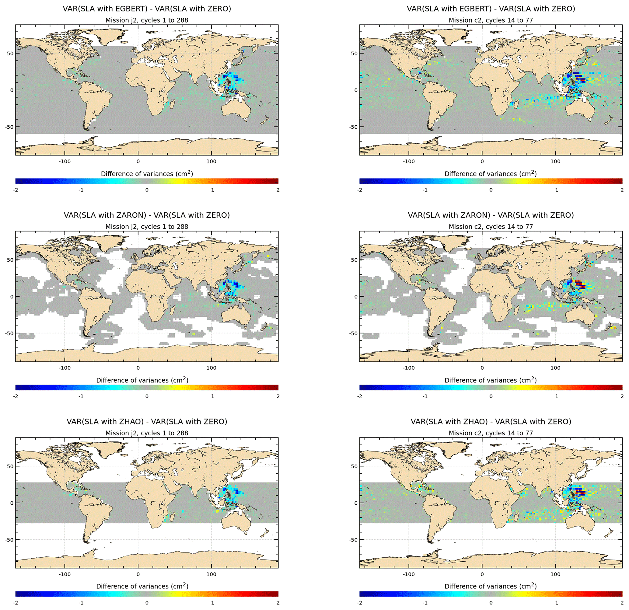
Figure B1Maps of SLA variance differences using either the O1 IT correction from each model or a reference ZERO correction in the SLA calculation for the J2 and C2 missions (cm2). J2 cycles 1–288 have been used; C2 cycles 14–77 have been used.
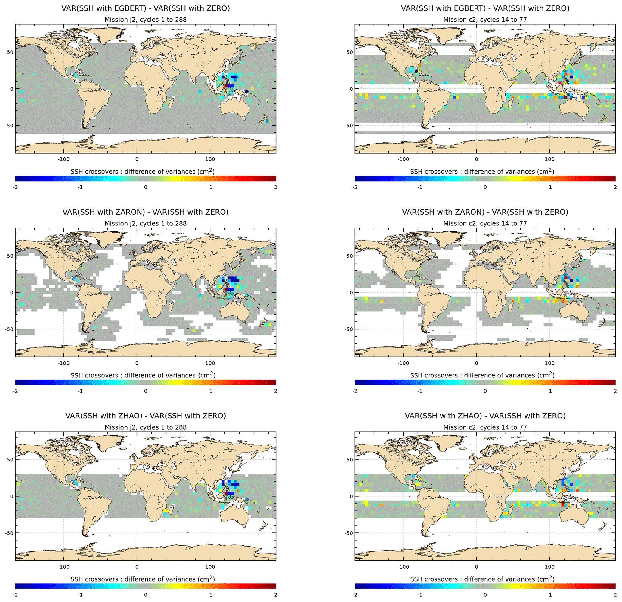
Figure B2Maps of SSH variance differences at crossovers using either the O1 IT correction from each model or a reference ZERO correction in the SSH calculation for the J2 and C2 missions (cm2). J2 cycles 1–288 have been used; C2 cycles 14–77 have been used.
The maps of SLA and crossover variance differences using each of the three different S2 IT models are plotted in Figs. C1 and C2, respectively, for both J2 and C2 missions; the S2 IT solutions are compared to a ZERO reference correction. The ZARON S2 solution is not defined in large deep-ocean regions (white areas in the maps) where the S2 IT amplitude is negligible and/or not separable from background ocean variability.
Using the three models for S2 IT correction allows a small but well-detected reduction in the J2 and C2 SLA variances in the same regions of the ocean as for the main semidiurnal IT (see Figs. 7–10 for M2 IT): variance reduction is maximal (about 0.5–1 cm2) west of the Hawaii region, north of Madagascar, in the Luzon Strait or west Pacific region and also in the Indonesian islands, north of Sumatra, and between the Solomon Islands and New Zealand. The C2 maps show similar reduction patterns, but the variance gain is weaker than for J2. Both the EGBERT and ZHAO models remove some variance south of Africa in the Agulhas currents, while ZARON does not; the ZHAO model clearly impacts the altimeter variance in most of the great ocean currents areas, which likely indicates that the model might contain some residual oceanic signal and/or some J2 error and not only IT. The patterns of the crossover variance differences are consistent for J2 missions but with weaker values than for the SLA; for the C2 mission, the crossover maps indicate a weaker and noisier impact than for SLA as already noted for the O1 frequency.
The mean statistics of the altimeter variance reduction are gathered in table C3 for the SLA and the SSH differences of the J2 and C2 missions and for the different regions studied; the analysis focuses on Tahiti, Hawaii, NPAC, Madagascar and the Luzon areas because mean S2 statistics are not significant elsewhere. The figures show weak SLA variance reductions with stronger values in the Luzon, Madagascar and Hawaii regions, where the amplitude of the S2 IT is the most important: if looking at J2 SLA, the three models are equivalent in Hawaii and Madagascar, but EGBERT and ZARON are more efficient at reducing variance in the Luzon area (0.28 and 0.25 cm2, respectively). Looking at C2 SLA, the three models give similar results in Madagascar, EGBERT and ZHAO reduce more variance in the Luzon region, and EGBERT is more efficient in the Hawaii region. Unlike the results obtained for the M2 and K1 waves and described in previous sections, the variance reduction for crossover differences is weaker than for the SLA for the S2 wave and mean values are hardly useful; this is likely explained by the weak S2 IT signal in the ocean in addition to the fact that crossover statistics are performed in large boxes, which tends to smooth them even more. This analysis results suggest that the EGBERT and ZARON S2 IT solutions are the most efficient in the different regions of interest.
Table C1Mean variance reduction for J2 and C2 altimeter databases, within each IT region, when using the different S2 internal-tide models and compared to the ZERO correction case; variance reduction in altimeter SLA (white lines) and for altimeter crossover differences (italic lines) for each mission, in square centimeters (0 is for < 0.005 cm2). For each IT region, the maximum variance reduction across the different models is highlighted in bold.

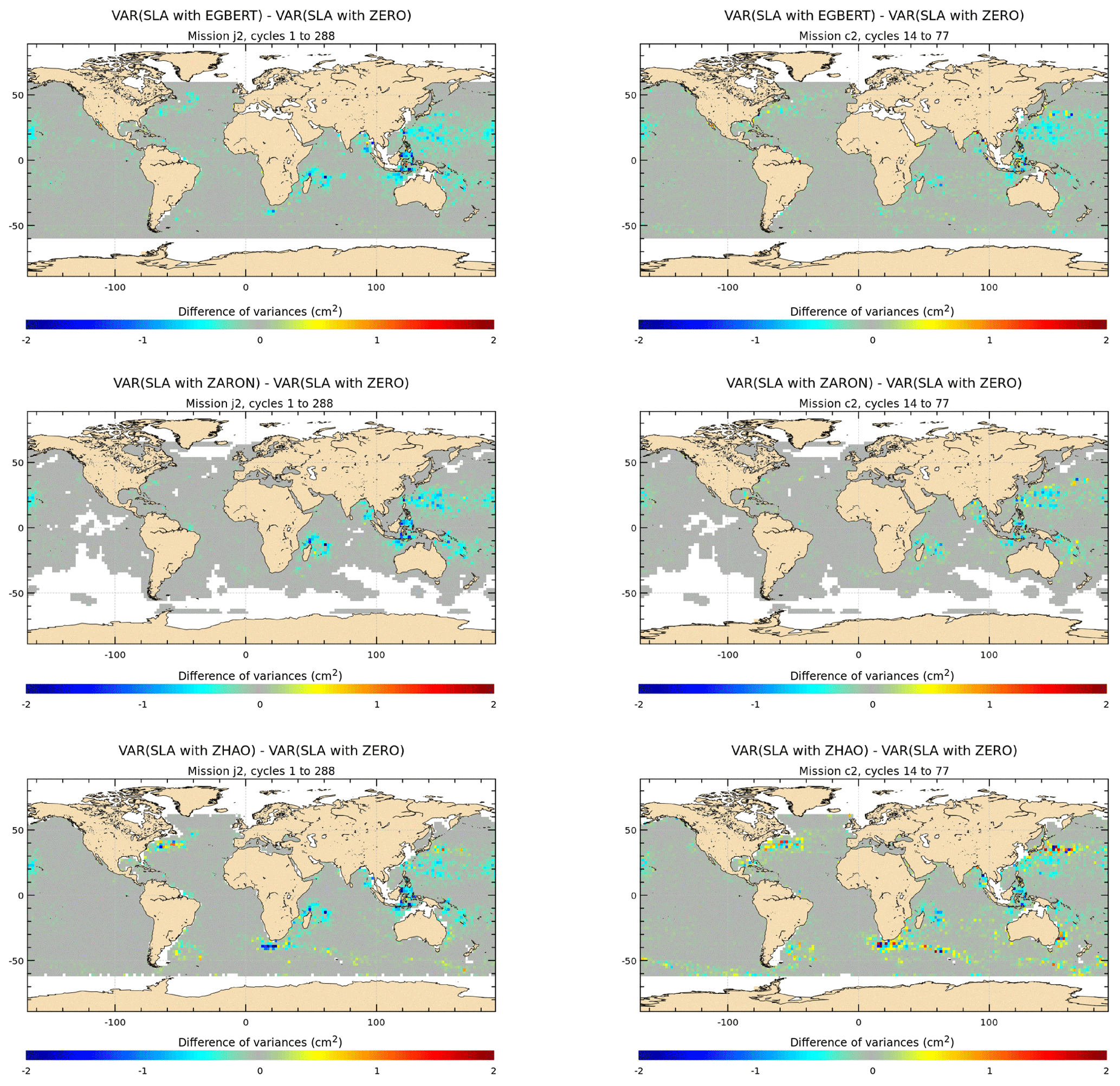
Figure C1Maps of SLA variance differences using either the S2 IT correction from each model or a reference ZERO correction in the SLA calculation for the J2 and C2 missions (cm2). J2 cycles 1–288 have been used; C2 cycles 14–77 have been used.
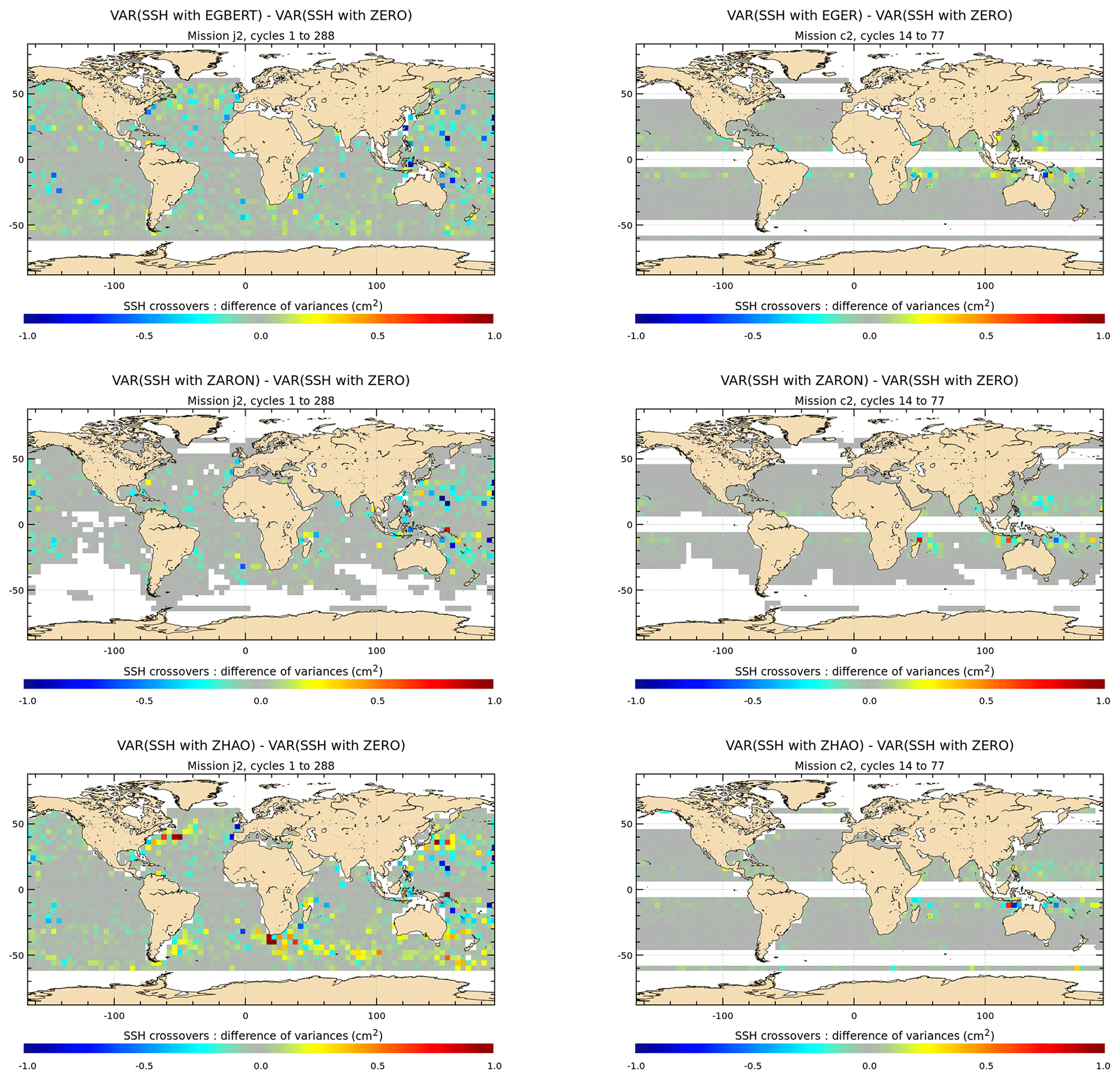
Figure C2Maps of SSH variance differences at crossovers using either the S2 IT correction from each model or a reference ZERO correction in the SSH calculation for the J2 and C2 missions (cm2). J2 cycles 1–288 have been used; C2 cycles 14–77 have been used.
Level 2P (L2P) altimetry products, with 1 Hz along-track resolution (LRM), are produced and distributed by Aviso+, as part of the Ssalto ground processing segment (https://www.aviso.altimetry.fr/en/data/, last access: 8 January 2021). The version of the L2P products used in the present study corresponds to the DT-2014 standards described in Pujol et al. (2016), except for the tide correction. The FES2014b global tidal atlas is available at the Aviso+ web page (https://www.aviso.altimetry.fr/en/data/products/auxiliary-products/global-tide-fes.html, last access: 8 January 2021). MSS_CNES_CLS_11 referenced on the 20-year altimetric period is also available at the Aviso+ web page (https://www.aviso.altimetry.fr/en/data/products/auxiliary-products/mss.html, last access: 8 January 2021). Brian Dushaw's baroclinic tide model can be downloaded at https://apl.uw.edu/project/project.php?id=tm_1-15 (last access: 8 January 2021). The latest version of Edward Zaron's baroclinic tide model can be downloaded at https://ezaron.hopto.org/~ezaron/downloads.html (last access: 8 January 2021); HRET version 7.0 was used for the present study. Other baroclinic tide models have been provided specifically by the authors for the present study and are not publicly available, but they might be provided by their respective authors on demand.
The supplement related to this article is available online at: https://doi.org/10.5194/os-17-147-2021-supplement.
BKA, BD, GE, SE, RDR, CU, EZ, ZZ, JFS and MCB provided the different IT models that have been used for the study. LC designed the experiments and carried them out with the help of the CLS team. LC analyzed the results with contributions from all co-authors. LC prepared the paper with contributions from all co-authors.
The authors declare that they have no conflict of interest.
This article is part of the special issue “Developments in the science and history of tides (OS/ACP/HGSS/NPG/SE inter-journal SI)”. It is not associated with a conference.
This work has been performed within the framework of the SWOT-ADT (Algorithm Definition Team) and funded by CNES. We thank Romain Baghi for his help in the processing.
This paper was edited by Mattias Green and reviewed by C. K. Shum and one anonymous referee.
Ablain M., Legeais, J. F., Prandi, P., Fenoglio-Marc, L., Marcos, M., Benveniste, J., and Cazenave, A.: Altimetry-based sea level, global and regional, Surv. Geophys., 38, 7–31, https://doi.org/10.1007/s10712-016-9389-8, 2016.
Ansong, J. K., Arbic, B. K., Buijsman, M. C., Richman, J. G., Shriver, J. F., and Wallcraft, A. J.: Indirect evidence for substantial damping of low-mode internal tides in the open ocean, J. Geophys. Res.-Oceans, 120, 6057–6071, https://doi.org/10.1002/2015JC010998, 2015.
Antonov, J. I., Seidov, D., Boyer, T. P., Locarnini, R. A., Mishonov, A. V., Garcia, H. E., Baranova, O. K., Zweng, M. M., and Johnson, D. R.: World Ocean Atlas 2009, Vol. 2, Salinity, edited by: Levitus, S., NOAA Atlas NESDIS 69, U.S. Government Printing Office, Washington, DC, 184 pp., 2010.
AVISO: Archiving Validation and Interpretation of Satellite Oceanographic data, available at: https://www.aviso.altimetry.fr/en/data/products/sea-surface-height-products/global/along-track-sea-level-anomalies-l2p.html, last access: 17 December 2020.
Barbot, S., Lyard, F., Tchilibou, M., and Carrere, L.: The dependency of internal tidal waves on stratification temporal variability, in preparation, 2020.
Buijsman, M. C., Arbic, B. K., Richman, J. G., Shriver, J. F., Wallcraft, A. J., and Zamudio, L.: Semidiurnal internal tide incoherence in the equatorial Pacific, J. Geophys. Res.-Oceans, 122, 5286–5305, https://doi.org/10.1002/2016JC012590, 2017.
Buijsman, M. C., Stephenson, G. R., Ansong, J. K., Arbic, B. K., Green, J. A. M.,Richman, J. G., Shriver, J. F., Vic, C., Wallcraft, A. J., and Zhao, Z.: On the interplay between horizontal resolution and wave drag and their effect on tidal baroclinic mode waves in realistic global ocean simulations, Ocean Model., 152, https://doi.org/10.1016/j.ocemod.2020.101656, 2020.
Carrere, L. and Lyard, F.: Modeling the barotropic response of the global ocean to atmospheric wind and pressure forcing-comparisons with observations, Geophys. Res. Lett., 6, 8-1–8-4, 2003.
Carrere, L., Le Provost, C., and Lyard, F.: On the statistical stability of the M2 barotropic and baroclinic tidal characteristics from along-track TOPEX/Poseidon satellite altimetry analysis, J. Geophys. Res.-Oceans, 109, C03033, https://doi.org/10.1029/2003JC001873, 2004.
Carrere, L., Lyard, F., Cancet, M., Guillot, A., and Picot, N.: FES 2014, a new tidal model – Validation results and perspectives for improvements, ESA Living Planet Conference, Prague, Czech Republic, 2016a.
Carrere, L., Faugère, Y., and Ablain, M.: Major improvement of altimetry sea level estimations using pressure-derived corrections based on ERA-Interim atmospheric reanalysis, Ocean Sci., 12, 825–842, https://doi.org/10.5194/os-12-825-2016, 2016b.
Chelton, D. B., Deszoeke, R. A., Schlax, M. G., El Naggar, K., and Siwertz, N.: Geographical variability of the first baroclinic Rossby radius of deformation, J. Phys. Oceanogr., 28, 433–460, 1998.
Dushaw, B. D.: Mapping low-mode internal tides near Hawaii using TOPEX/POSEIDON altimeter data, Geophys. Res. Lett., 29, 911–914. https://doi.org/10.1029/2001GL013944, 2002.
Dushaw, B. D.: Mode-1 internal tides in the western North Atlantic, Deep-Sea Res., 53, 449–473, https://doi.org/10.1016/j.dsr.2005.12.009, 2006.
Dushaw, B. D.: An Empirical Model for Mode-1 Internal Tides Derived from Satellite Altimetry: Computing Accurate Tidal Predictions at Arbitrary Points over the World Oceans, Technical Memorandum APL-UW TM, available at: http://www.apl.washington.edu/project/projects/tm_1-15/pdfs/tm_1_15.pdf (last access: 17 December 2020), 2015.
Dushaw, B. D., Worcester, P. F., Cornuelle, B. D., Howe, B. M., and Luther, D. S.: Baroclinic and barotropic tides in the central North Pacific Ocean determined from long-range reciprocal acoustic transmissions, J. Phys. Oceanogr., 25, 631–647, 1995.
Dushaw, B. D., Worcester, P. F., and Dzieciuch, M. A.: On the predictability of mode-1 internal tides, Deep-Sea Res., 58, 677–698, https://doi.org/10.1016/j.dsr.2011.04.002, 2011.
Dushaw, B. D., Gaillard, F., and Terre, T.: Acoustic tomography in the Canary Basin: Meddies and tides, J. Geophys. Res.-Oceans, 122, 8983–9003, https://doi.org/10.1002/2017JC013356, 2017.
Egbert, G. D. and Erofeeva, S. Y.: Efficient inverse modeling of barotropic ocean tides, J. Atmos. Oceanic Technol., 19, 183–204, 2002.
Egbert, G. D. and Erofeeva, S. Y.: Mapping M2 Internal Tides Using a Data-Assimilative Reduced Gravity Mode, AGU Fall Meeting, 2014AGUFMOS43F..01E, 2014.
Egbert, G. D. and Ray, R. D.: Significant dissipation of tidal energy in the deep ocean inferred from satellite altimeter data, Nature, 15, 6788, https://doi.org/10.1038/35015531, 2000.
Escudier, P., Couhert, A., Mercier, F., Mallet, A., Thibaut, P., Tran, N., Amarouche, L., Picard, B., Carrere, L., Dibarboure, G., Ablain, M., Richard, J., Steunou, N., Dubois, P., Rio, M.-H., and Dorandeu, J.: Satellite Radar Altimetry – Principle, Accuracy, and Precision, in: Satellite Altimetry Over Oceans and Land Surfaces, edited by: Stammer, D. and Cazenave, A., 1st Edn., CRC Press, Boca Raton, 643 pp., https://doi.org/10.1201/9781315151779, 2017.
Faugère, Y., Durand, C., Carrere, L., Ubelmann, C., Ballarotta, M., and Dibarboure, G.: Impact of internal tide correction on the DUACS maps accuracy, available at: https://meetings.aviso.altimetry.fr/fileadmin/user_upload/2019/TID_01_DUACS_IT_Impact-Faugere.pdf (last access: 17 December 2020), 2019.
Griffiths, S. D. and Grimshaw, R. H. J.: Internal Tide Generation at the Continental Shelf Modeled Using a Modal Decomposition: Two-Dimensional Results, J. Phys. Oceanogr., 37, 428–451, https://doi.org/10.1175/JPO3068.1, 2007.
Locarnini, R. A., Mishonov, A. V., Antonov, J. I., Boyer, T. P., Garcia, H. E., Baranova, O. K., Zweng, M. M, and Johnson, D. R.: World Ocean Atlas 2009, Vol. 1, Temperature, in: NOAA Atlas NESDIS 68, edited by: Levitus, S., U.S. Government Printing Office, Washington, D.C., USA, 184 pp., 2010.
Luecke, C.A., Arbic, B. K., Bassette, S. L., Richman, J.,G., Shriver, J. F., Alford, M. H., Smedstad, O. M., Timko, P. G., Trossman, D. S., and Wallcraft, A. J.: The global mesoscale eddy available potential energy field in models and observations, J. Geophys. Res.-Oceans, 122, 9126–9143, https://doi.org/10.1002/2017JC013136, 2017.
Lyard, F., Lefevre, F., Letellier, T., and Francis, O.: Modelling the global ocean tides: Modern insights from FES2004, Ocean Dyn., 56, 394–415, 2006.
Lyard, F. H., Allain, D. J., Cancet, M., Carrere, L., and Picot, N.: FES2014 global ocean tides atlas: design and performances, Ocean Sciences Discussions, 1–40, https://doi.org/10.5194/os-2020-96, 2020.
Ngodock, H. E., Souopgui, I., Wallcraft, A. J., Richman, J. G., Shriver, J. F., and Arbic, B. K.: On improving the accuracy of the M2 barotropic tides embedded in a high-resolution global ocean circulation model, Ocean Model., 97, 16–26, https://doi.org/10.1016/j.ocemod.2015.10.011, 2016.
Nugroho D.: the tides in a general circulation model in the Indonesian Seas, PhD thesis, Uuniversité de Toulouse, UT3 Paul Sabatier, France, 226 pp., 2017.
Pujol, M.-I., Faugère, Y., Taburet, G., Dupuy, S., Pelloquin, C., Ablain, M., and Picot, N.: DUACS DT2014: the new multi-mission altimeter data set reprocessed over 20 years, Ocean Sci., 12, 1067–1090, https://doi.org/10.5194/os-12-1067-2016, 2016.
Quartly, G. D., Legeais, J.-F., Ablain, M., Zawadzki, L., Fernandes, M. J., Rudenko, S., Carrère, L., García, P. N., Cipollini, P., Andersen, O. B., Poisson, J.-C., Mbajon Njiche, S., Cazenave, A., and Benveniste, J.: A new phase in the production of quality-controlled sea level data, Earth Syst. Sci. Data, 9, 557–572, https://doi.org/10.5194/essd-9-557-2017, 2017.
Rainville, L. and Pinkel, R.: Propagation of Low-Mode Internal Waves through the Ocean, J. Phys. Oceanogr., 36, 1220–1236, https://doi.org/10.1175/JPO2889.1, 2006.
Ray, R. D.: Precise comparisons of bottom-pressure and altimetric ocean tides, J. Geophys. Res.-Oceans, 118, 4570–4584, https://doi.org/10.1002/jgrc.20336, 2013.
Ray, R. D., and Mitchum, G. T.: Surface manifestation of internal tides in the deep ocean: Observations from altimetry and island gauges, Prog. Oceanogr., 40, 135–162, 1997.
Ray, R. D. and Zaron, E. D.: M2 Internal Tides and Their Observed Wavenumber Spectra from Satellite Altimetry, J. Phys. Oc., 46, 3–22, https://doi.org/10.1175/JPO-D-15-0065.1, 2016.
Schaeffer P., Faugere, Y., Legeais, J.F., Picot, N., and Bronner, E.: The CNES_tCLS11 Global Mean Sea Surface computed from 16 years of satellite altimeter data, Mar. Geod., 35, 3–19, https://doi.org/10.1080/01490419.2012.718231, 2012.
Shriver, J. F., Richman, J. G., and Arbic, B. K.: How stationary are the internal tides in a high-resolution global ocean circulation model?, J. Geophys. Res.-Oceans, 119, 2769–2787, https://doi.org/10.1002/2013JC009423, 2014.
Shum C. K., Woodworth, P. L., Andersen, O. B., Egbert, G. D., Francis, O., King, C., Klosko, S. M., Le Provost, C., Li, X., Molines, J.-M., Parke. M. E., Ray, R. D., Schlax, M. G., Stammer, D., Tiemey, C. C., Vincent, P., and Wunsch, C. I.: Accuracy assessment of recent ocean tide models, JGR Oceans, 102194, https://doi.org/10.1029/97JC00445, 1997.
Smith, W. H. F. and Sandwell, D. T.: Global seafloor topographyfrom satellite altimetry and 313 ship depth soundings, Science, 277, 1957–1962, 1997.
Stammer, D., Ray, R. D., Andersen, O. B., Arbic, B. K., Bosch, W., Carrere, L., Cheng, Y., Chinn, D. S., Dushaw, B. D., Egbert, G. D., Erofeeva, S. Y., Fok, H. S., Green, J. A. M., Griffiths, S., King, M. A., Lapin, V., Lemoine, F. G., Luthcke, S. B., Lyard, F., Morison, J., Müller, M., Padman, L., Richman, J. G., Shriver, J. F., Shum, C. K., Taguchi, E., and Yi, Y.: Accuracy assessment of global barotropic ocean tide models, Rev. Geophys., 52, 243–282, https://doi.org/10.1002/2014RG000450, 2014.
Taburet, G., Sanchez-Roman, A., Ballarotta, M., Pujol, M.-I., Legeais, J.-F., Fournier, F., Faugere, Y., and Dibarboure, G.: DUACS DT2018: 25 years of reprocessed sea level altimetry products, Ocean Sci., 15, 1207–1224, https://doi.org/10.5194/os-15-1207-2019, 2019.
Tailleux, R. and McWilliams, J. C.: The effect of bottom pressure decoupling on the speed of extratropical, baroclinic Rossby waves, J. Phys. Oceanogr., 31, 1461–1476, 2001.
Zaron, E. D.: Mapping the nonstationary internal tide with satellite altimetry, J. Geophys. Res.-Oceans, 122, 539–554, https://doi.org/10.1002/2016JC012487, 2017.
Zaron, E. D.: Baroclinic Tidal Sea Level from Exact-Repeat Mission Altimetry, J. Phys. Oceanogr., 49, 193–210, https://doi.org/10.1175/JPO-D-18-0127.1, 2019.
Zaron, E. D. and Ray, R. D.: Aliased Tidal Variability in Mesoscale Sea Level Anomaly Maps, J. Atmos. Oceanic Technol., 35, 2421–2435, https://doi.org/10.1175/JTECH-D-18-0089.1, 2018.
Zhao, Z.: Mapping Internal Tides From Satellite Altimetry Without Blind Directions, J. Geophys. Res.-Oceans, 124, 8605–8625, https://doi.org/10.1029/2019JC015507, 2019a.
Zhao, Z.: Temporal variability of the mode-1 M2 internal tide, Chicago OSTST meeting, available at: https://meetings.aviso.altimetry.fr/programs/2019-ostst-complete-program.html (last access: 21–25 October 2020), 2019b.
Zhao, Z., Alford, M. H., and Girton, J. B.: Mapping low-mode internal tides from multisatellite altimetry, Oceanography, 25, 42–51, 2012.
- Abstract
- Introduction
- Presentation of participating internal-tide models
- Comparison of internal-tide models
- Presentation of the altimeter database and the method of comparison
- Variance reduction analysis using satellite altimeter data
- Wavelength analysis for the M2 wave
- Discussion
- Appendix A: Comparing internal-tide models for O1 and S2 waves
- Appendix B: Validation results for O1 IT models
- Appendix C: Validation results for S2 IT models
- Data availability
- Author contributions
- Competing interests
- Special issue statement
- Acknowledgements
- Review statement
- References
- Supplement