Evaluating high-frequency radar data assimilation impact in coastal ocean operational modelling

The impact of the assimilation of HFR (high-frequency radar) observations in a high-resolution regional model is evaluated, focusing on the improvement of the mesoscale dynamics. The study area is the Ibiza Channel, located in the western Mediterranean Sea. The resulting fields are tested against trajectories from 13 drifters. Six different assimilation experiments are compared to a control run (no assimilation). The experiments consist of assimilating (i) sea surface temperature, sea level anomaly, and Argo profiles (generic observation dataset); the generic observation dataset plus (ii) HFR total velocities and (iii) HFR radial velocities. Moreover, for each dataset, two different initialization methods are assessed: (a) restarting directly from the analysis after the assimilation or (b) using an intermediate initialization step applying a strong nudging towards the analysis fields. The experiments assimilating generic observations plus HFR total velocities with the direct restart provide the best results, reducing by 53 % the average separation distance between drifters and virtual particles after the first 48 h of simulation in comparison to the control run. When using the nudging initialization step, the best results are found when assimilating HFR radial velocities with a reduction of the mean separation distance by around 48 %. Results show that the integration of HFR observations in the data assimilation system enhances the prediction of surface currents inside the area covered by both antennas, while not degrading the correction achieved thanks to the assimilation of generic data sources beyond it. The assimilation of radial observations benefits from the smoothing effect associated with the application of the intermediate nudging step.

1 Introduction

High-frequency radar (HFR) is a fast-growing technology, playing an important role in coastal observing systems around the world (Roarty et al., 2019; Rubio et al., 2017). It allows real-time measurements providing a new, detailed, and quantitative description of physical processes at the marine surface (Paduan and Washburn, 2013). Its capacity to measure currents at high spatial and temporal resolution over relatively large coastal areas makes it a convenient system for operational purposes. It can be used to validate numerical models (Aguiar et al., 2019; Mourre et al., 2018; Lorente et al., 2021), analyse Lagrangian dynamics (Hernández-Carrasco et al., 2018), or constrain numerical models via data assimilation (DA) (Vandenbulcke et al., 2017; Iermano et al., 2016; Janeković et al., 2020).

HFR is a cost-effective shore-based remote-sensed technology exploiting the Bragg resonance phenomenon (Crombie, 1955) to map ocean surface currents, wave fields, and increasingly winds in coastal areas. It complements satellite altimeter observations, which are limited to larger scales and suffer limitations when approaching the coast (Vignudelli et al., 2019; Pascual et al., 2013). The capability of HFR to give realistic observations of surface currents has been widely validated (Chapman et al., 1997; Emery et al., 2004; Paduan et al., 2006). Furthermore it has been used to validate geostrophic currents computed from along-track altimetry (Pascual et al., 2015) and to correct sea surface height (SSH) altimeter fields (Roesler et al., 2013).

Regional ocean models are invaluable tools for operational oceanography (Wilkin and Hunter, 2013; Onken et al., 2008; De Mey-Frémaux et al., 2019). However, they are inevitably affected by errors from multiple sources, especially in highly dynamic coastal areas where conditions tend to change rapidly. In such places, the assimilation of observations such as the ones provided by HFR can help to constrain the model solution and improve the forecast. Assimilation of HFR data has been successfully applied in different regions around the globe, starting from the pioneer study conducted by Breivik (2001) using an optimal interpolation (OI) scheme. Since then, many different studies have explored the performance of HFR for data assimilation in ocean circulation models using different assimilation schemes, data types, and techniques. Authors have employed high-frequency (hourly) or filtered data depending on the focus of the study and the dynamical processes of interest. The use of radial or total observations has also been the subject of study and debate. While radial velocities theoretically provide a larger amount of information without any data processing, they are prone to present higher spatial gradients than reconstructed total observations, which incorporate some spatial smoothing. In addition, radials have a wider coverage, providing data in areas only covered by one antenna and can be used even in the case of failure of the other antennas. Theoretically, under the assumptions of linearity and normal distribution of errors in the state dynamics and measurements, as well as in the transformation from radials to totals, the assimilation of radial currents should outperform the assimilation of total currents, since all the information of the totals is included in the radials and the latter contain additional information that is not included in the totals. However, in real-world experiments, these major assumptions are not verified. In particular, the model is non-linear, observation error covariances are not Gaussian and certainly not perfectly known, and the transformation from radials to totals also involves non-linearities. In the literature, both kinds of observations have been assimilated with satisfactory results. To our knowledge, Shulman and Paduan (2009) is the only work evaluating the contribution of both radial and total velocities in the same experiment. Their results show the capacity of the system to improve surface currents and circulation down to 120 m depth in areas covered by two or more antennas for both kinds of data. Depending on the position of the mooring with respect to the coverage of the antennas, their validation showed a varying complex correlation against mooring observations when using radial or total observations. Using observations from only one antenna, Shulman and Paduan (2009) found that results were extremely variable and highly dependent on the direction of the bearing with respect to the dominant flow.

Oke et al. (2002) used an OI scheme to assimilate low-pass filtered surface total velocity measurements from an HFR array to correct model circulation. They used a so-called TDAP (time-distributed averaging procedure) initialization method after analysis, which progressively applies data assimilation increments to preserve appropriate dynamical balances. This data assimilation approach resulted in an increase of the correlation between model and observations from 0.42 to 0.78.

More recently, hourly reconstructed total currents have also been employed using both sequential (Ren et al., 2016; Paduan and Shulman, 2004) and variational data assimilation schemes such as 4D-Var (Zhang et al., 2010; Wilkin and Hunter, 2013; Yu et al., 2016). However, depending on the model setup and the oceanic processes of interest, the use of hourly data may not be the most appropriate, as for instance in Kerry et al. (2016), where radial speeds and angles are spatially averaged onto the model grid and a 24 h boxcar-averaging filter is used to remove tides and inertial oscillations that are not resolved by the model. Kerry et al. (2018) show that among all the assimilated observations, HFR were the ones that had the larger impact on the currents and the transport in the Eastern Australian Current.

The use of hourly data in sequential data assimilation schemes is not straightforward, due to the analysis frequency, which is generally larger than 1 h. An option is to use an extended state vector as in Barth et al. (2008), who employed an ensemble based Kalman filter (KF) method using hourly radial observations in the West Florida Shelf. For the initialization, Barth et al. (2008) implemented a spatial filter and averaged the ensemble fields in an attempt to remove spurious variability before it is introduced into the model. Barth et al. (2011) and Marmain et al. (2014) employed a similar approach, using all radial hourly observations available during the assimilation window and an extended state vector to correct the wind forcing fields and boundary conditions, respectively, in a similar way to variational methods. While Barth et al. (2011) showed that the correction had a positive impact on the reconstructed winds and the sea surface temperature (SST) in the German Bight, Marmain et al. (2014) found an improvement in surface currents in the north-western Mediterranean Sea, although with some degradation on the density fields and under surface currents. Stanev et al. (2015) also used hourly radial observations to correct tidal currents in the German Bight. In an operational context and based on a spatio-temporal optimal interpolation (STIO), Stanev et al. (2016) demonstrated that their system had a good skill to correct currents even beyond the HFR covered area.

A comparison of the impact of both time-filtered and unfiltered HFR currents (with respect to a model with and without tides) was done in Shulman and Paduan (2009), showing that the sub-tidal period velocity simulations were similarly improved through the assimilation of either low-pass-filtered surface currents or instantaneous (hourly) surface currents. More recently, Vandenbulcke et al. (2017), using different KF schemes with an extended state vector, assimilated hourly radial velocities to correct inertial oscillations in a regional model of the Ligurian Sea. They showed an important effect on the correction of inertial oscillations during the first 12 h when considering all hourly observations in a 48 h time window instead of using only those corresponding to one single hour.

In the present study, we aim to evaluate the impact on coastal ocean operational modelling of the assimilation of both HFR total and radial velocities, and also to exploit different initialization methods after analysis. Our focus is on the correction of mesoscale structures and larger scale circulation, rather than inertial oscillations or tidal currents.

The study area is the Ibiza Channel (IC; Fig. 1), which is the passage between the oriental coast of Spain's mainland and the island of Ibiza. It is a crucial area for understanding mixing and transport processes in the north-western Mediterranean Sea. Two different water masses interact in the IC: (i) relatively salty water that has already recirculated in the western Mediterranean flowing southward along the shelf as the Northern Current and (ii) a branch of the Modified Atlantic Water transporting fresher waters originally entering through the Strait of Gibraltar and flowing northward (Pinot et al., 1994, 1995) on its easternmost part. The dynamics and the ecological and economical importance of the area have raised a specific interest in understanding the relevant ocean processes (Heslop et al., 2012; Balbín et al., 2014; Pinot et al., 2002; Hernández-Carrasco et al., 2018; Vargas-Yáñez et al., 2021). The analysis of repeated observations along a glider endurance line in the Ibiza Channel has revealed a high variability of meridional transports over timescales of days to weeks (Heslop et al., 2012). This high variability due to the interaction of multiple processes with different water masses over a complex topography make the operational forecasting particularly challenging. The anthropogenic pressure in the region makes it necessary to develop accurate tools for search and rescue, oil spill forecasting, or larval dispersion to efficiently respond to emergencies and protect ecosystems.

Since 2012, the Balearic Island Coastal Observing and forecasting System (SOCIB; Tintoré et al., 2013) has operated a CODAR HFR system that monitors the IC with two antennas measuring hourly surface currents (Tintoré et al., 2020). This infrastructure is part of the Joint European Research Infrastructure of coastal observatories (JERICO; https://www.jerico-ri.eu, last access: 12 August 2021). Lana et al. (2016) validated the IC HFR observations against a current meter, acoustic doppler current profiler (ADCP), and surface Lagrangian drifters, showing a good agreement and the absence of significant mean error (hereafter referred to as bias). A joint analysis of HFR observations and surface winds in terms of empirical orthogonal functions (EOFs) demonstrated that the surface current variability was mainly driven by local winds and mesoscale circulation.

The present research on Ibiza Channel HFR data assimilation was carried out within the Joint Research Action on coastal forecasting of the European Horizon 2020 JERICO-NEXT project. Seven 1 month simulations have been generated to investigate the data assimilation performance of HFR raw radial observations compared to reconstructed total currents. We have employed three different datasets and for each of them two different initialization methods after analysis. Additionally, a free-run simulation without assimilation was used as a control run. An exhaustive assessment was performed following both Eulerian and Lagrangian approaches, including an independent set of 13 drifters deployed in the area.

The paper is structured as follows: Sect. 2 describes the data and methods employed, including the DA system and the description of the experiments. The results are presented in Sect. 3. Finally, the discussion of the results and the conclusions are presented in Sects. 4 and 5.

2 Data and methods

2.1 High-frequency radar

The SOCIB HFR system consists of two CODAR SeaSonde stations on the islands of Ibiza and Formentera (named GALF and FORM, respectively), covering the eastern side of the IC. It has operated since June 2012, providing real-time high-resolution observations of surface currents (Tintoré et al., 2020; Lana et al., 2015, 2016). Each HFR station emits at a central frequency of 13.5 MHz and a bandwidth of 90 kHz, reaching ranges up to 85 km. Emitted electromagnetic waves are backscattered by surface waves of exactly half the HFR wavelength. Radial velocities (velocities toward or away from the antenna) are derived from the Doppler shift due to the difference between ideal and measured Bragg frequency (Barrick, 2008). At the specified operating frequency, measurement depth is approximately 0.9 m (Stewart and Joy, 1974). Radial observations provide the velocity along a bearing calculated from radio signals backscattered from the ocean surface. Hourly radial velocity maps from both stations are systematically quality controlled and the total velocity vectors are reconstructed by combining the radial velocities with overlapping coverage on a regular 3×3 km grid. Each grid point observation is computed using a unweighted least square fitting (UWLS) (Lipa and Barrick, 1983) considering all radial observations within a 6 km radius. Total reconstructed observations have a range up to 65 km off the antenna, compared to the 85 km that radials can reach.

In our experiments, we used daily mean HFR observations (Fig. 1) to filter the high-frequency signals (i.e. tidal and inertial motions) and focus on correcting the sub-tidal processes. Notice that tides in this area have very low amplitudes on the order of only a few centimetres. Daily means of radial and total currents are computed independently for each data type from the hourly observations. For the total currents, the daily mean is only considered at grid points where, during each day, at least 50 % of hourly measurements are both available and flagged as good, as was also used by Lorente et al. (2015). In the case of the radials, we considered a threshold of 25 % for computing the daily mean.

As stated above, at each grid point, the hourly total currents are calculated using all available radial observations within a radius of 6 km. Consequently, some total observations could be computed using different radial grid points within this radius for each hour that individually do not satisfy the threshold of 50 % imposed for the total velocities. Therefore, using the same threshold to calculate the daily means of both observations could lead to patches with available reconstructed daily mean total currents but no daily mean radials available. This is why we decided to use a less restrictive threshold for radials to have better spatial coverage, consistent with that of the total observations in the area covered by both antennas.

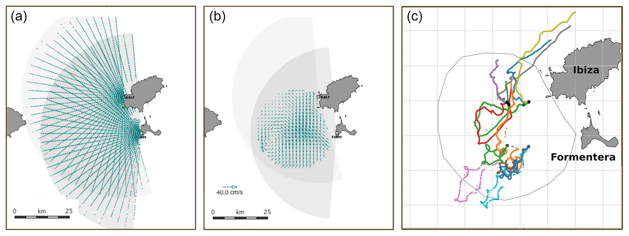
Figure 1 Map of the Ibiza Channel showing the HFR coverage area for radial (a) and total (b) currents, together with the position of the two antennas (GALF and FORM). Panel (c) shows the 13 drifters used for validation and their trajectories within the first 6 d after deployment. Each drifter has a randomly assigned colour. Dots indicate start locations of the trajectories.

2.2 Regional model configuration

The Western Mediterranean OPerational system (WMOP; Juza et al., 2016; Mourre et al., 2018) is a high-resolution regional configuration of the ROMS (Regional Ocean Modelling System) model (Shchepetkin and McWilliams, 2005) for the western Mediterranean Sea. The spatial coverage spans from the Strait of Gibraltar on the west to the Sardinia Channel on the east (6^∘ W–9^∘ E, 35–44.5^∘ N; see Fig. 1) with a horizontal resolution around 2 km and 32 vertical sigma levels (resulting in a vertical resolution between 1 and 2 m at the surface). The WMOP system is used to produce daily forecasts of the regional ocean circulation, which is used for a wide range of applications including search and rescue and analysis of plastic, parasite, or larval dispersion (Calò et al., 2018; Ruiz-Orejón et al., 2019; Cabanellas-Reboredo et al., 2019; Compa et al., 2020; Torrado et al., 2021; Kersting et al., 2020; Révelard et al., 2021).

The vertical mixing coefficients are set using the generic length scale (GLS) turbulence closure scheme (Umlauf and Burchard (2003); with parameters p=2.0, m=1.0, and $n=-\mathrm{0.67}$ as in line 1 of their Table 7). The bathymetry is derived from a 1^′ database (Smith and Sandwell, 1997). The simulation used in this study is initialized from and nested within the larger scale Copernicus Forecasting System (CMEMS MED-MFC) with a $\mathrm{1}/\mathrm{16}{}^{\circ }$ horizontal resolution (Simoncelli et al., 2017). The atmospheric forcing is provided every 3 h at $\mathrm{1}/\mathrm{20}{}^{\circ }$ resolution by the Spanish Meteorological Agency (AEMET) through the HIRLAM model (Undén et al., 2002). These fields are used to compute surface turbulent and momentum fluxes through bulk formulae. Atmospheric pressure forcing is neglected to avoid SSH high-frequency variability issues. Inflows from the six major rivers in the region are considered point sources using daily climatological values. Tides are not considered in the model.

A multi-year free-run hindcast spanning the period from 2009 to 2018 (Mourre et al., 2018; Aguiar et al., 2019) was used as a control simulation. This simulation also provides the initial state for the data assimilative simulations starting on 20 September 2014. Figure 2 shows the mean surface field of the control run during the simulation period (20 September to 20 October 2014) together with the mean surface currents measured by the HFR for the same period. The HFR observations depict an average southward current west of 0.8^∘ E. This current is deviated towards the south-east of 38.7^∘ N, and the flow is directed northward in the eastern side of the coverage area, close to the Ibiza and Formentera coast. The control run represents this overall pattern but with a significant overestimation of the mean velocities and a spatial mismatch of the eastward deviation of the flow (this deviation occurs too much to the east in the model).

2.3 Data assimilation system

The assimilation scheme employed here is the local multi-model Ensemble Optimal Interpolation (EnOI) employed in Hernández-Lasheras and Mourre (2018). It is a form of the EnOI that has been a widely used scheme since it represents a cost-effective alternative compared with more complex methods as the ensemble Kalman filter or the 4D-Var (Oke et al., 2002; Evensen, 2003; Counillon and Bertino, 2009). EnOI is a three-dimensional sequential assimilation method that allows the use of a large ensemble size together with localization. A stationary ensemble of model simulations is used to estimate background error covariances. The WMOP-DA system consists of a sequence of analyses (model updates given a set of observations) and model forward simulations.

For each analysis, the state vector $\mathit{x}=({\mathit{T}}_{i,j,k},{\mathit{S}}_{i,j,k},{\mathit{u}}_{i,j,k},{\mathit{v}}_{i,j,k},\mathit{S}\mathit{S}{\mathit{H}}_{i,j}{)}^T$ contains the model trajectory, i.e. the prognostic model variables at all wet grid points i, j, and k. During the analysis step, the state vector x^a is updated according to Eq. (1), where x^f is the background model state vector, H is the linear observation operator projecting the model state onto the observation space, and $\stackrel{\mathrm{̃}}{\mathbf{K}}$ is the Kalman gain estimated from the sample covariances (Eq. 2). y is the vector of observations. Matrices ${\stackrel{\mathrm{̃}}{\mathbf{P}}}^f$ and R are the error covariance matrices of the model and the observations, respectively.

$$\begin{array}{}\text{(1)}& {\displaystyle }{\mathit{x}}^a={\mathit{x}}^f+\stackrel{\mathrm{̃}}{\mathbf{K}}\left(\mathit{y}-\mathbf{H}{\mathit{x}}^f\right)\text{(2)}& {\displaystyle }\stackrel{\mathrm{̃}}{\mathbf{K}}={\stackrel{\mathrm{̃}}{\mathbf{P}}}^f{\mathbf{H}}^T{\left(\mathbf{H}{\stackrel{\mathrm{̃}}{\mathbf{P}}}^f{\mathbf{H}}^T+\mathbf{R}\right)}^{-\mathrm{1}}\end{array}$$

${\stackrel{\mathrm{̃}}{\mathbf{P}}}^f$ contains the background error covariances (BECs). In our approach, we estimated the BECs by sampling three long-run simulations of the WMOP with different initial and boundary forcings provided by the CMEMS MED-MFC (Simoncelli et al., 2017) and CMEMS GLO-MFC (Lellouche et al., 2018) forecasting systems and varying momentum and diffusion parameters. An ensemble of 80 realizations is considered in each analysis. Each ensemble member is randomly extracted from the three different long-run simulations within a temporal window of 90 d centred on the day of the analysis for the different years covered by the three long-run simulations. The seasonal cycle is removed from the multivariate fields before computing the ensemble anomalies to limit the effects of large-scale correlations, mainly in terms of surface temperature. This way, we obtain multivariate, inhomogeneous, and anisotropic three-dimensional model BECs characteristic of the mesoscale variability. We used a domain localization of 200 km corresponding to the average distance between two Argo profiles in the western Mediterranean Sea. An independent analysis is performed for each water column of the model domain considering only the observations within the localization radius.

We used a diagonal observation covariance error matrix R. The observation error for all HFR observations was considered the same, with a value of 0.1 m s⁻¹ (accounting for instrumental and representativity errors). This value is consistent with local comparisons against surface current measurements from a point-wise current meter (1.5 m depth) and a downward-looking ADCP (first bin at 5 m depth) carried out by Lana et al. (2016), which reported a RMSD between 0.07 and 0.12 m s⁻¹. This value of 0.1 m s⁻¹ was fixed in our experiments as it yielded a proper correction of surface currents without degrading the vertical structure. Once the observation error was set for HFR total observations, we performed new experiments to evaluate the potential differences between the total and radial observations. Total observations were interpolated and projected to generate synthetic radial observations containing the exact same information as the totals but with a radial-like pattern in the area covered by both antennas. The assimilation of these total and synthetic radial observations using the same observation error led to almost identical results in surface fields and vertical structure, with complex correlation of 0.92 and a RMSD of 0.02 m s⁻¹ obtained between both analysis fields in the HFR grid points. Based on these results, we decided to use the same observation error for both types of observations.

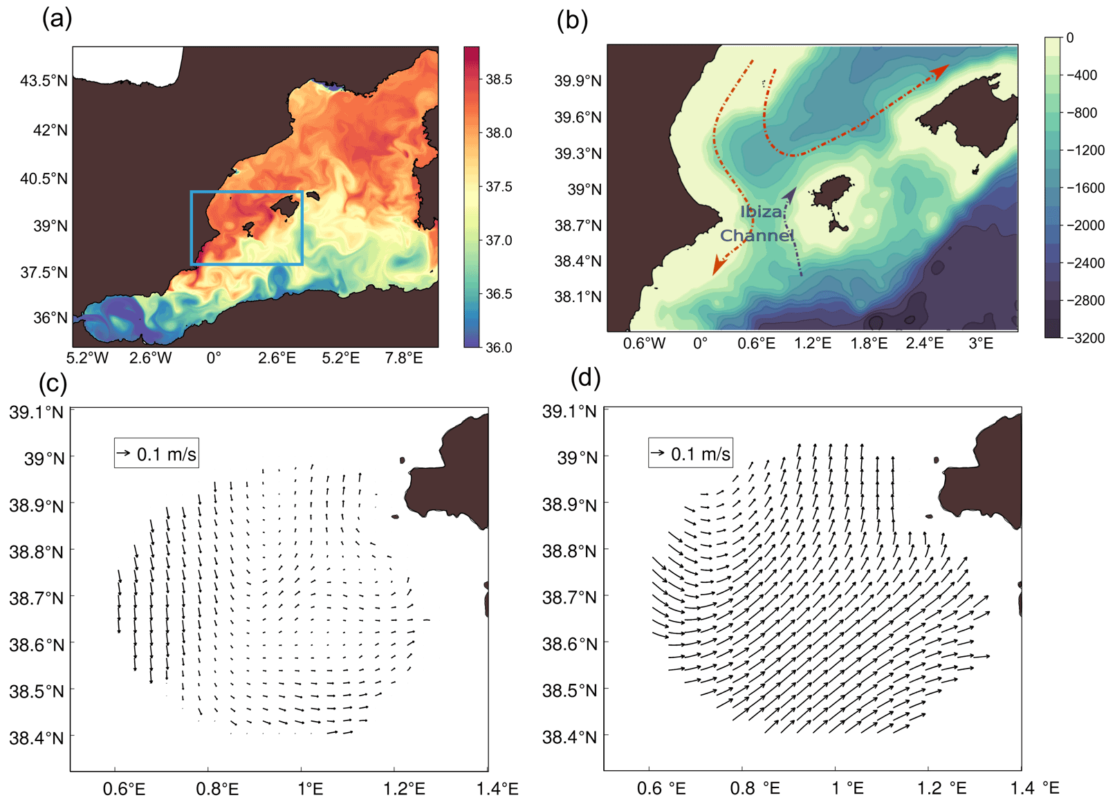
Figure 2 Illustration of the modelling domain and study area. (a) WMOP sea surface salinity (6 October 2014). The Ibiza and Mallorca Channel area is delimited by the blue rectangle. (b) Bathymetry (m) and main circulation features in the Ibiza Channel. (c) Mean HFR surface currents over the whole simulation period (20 September to 20 October 2014). (d) Mean surface currents over the whole simulation period computed from the model.

The state vector equivalents of HFR radials are obtained using the following equation:

$$\begin{array}{}\text{(3)}& \mathbf{H}{\mathit{x}}^f={\mathit{u}}_x\cos \mathit{\alpha }+{\mathit{u}}_y\sin \mathit{\alpha },\end{array}$$

where u_x and u_y are the model surface velocity components interpolated at the observation point and α denotes the angle (anti-clockwise towards the east) pointing from an antenna station to a certain location.

A 3 d assimilation cycle is applied with different time windows for each source of observation as explained in the following section. In each analysis (day n), the daily average field is employed as background and two different initialization approaches (Fig. 3) have been applied to restart the model after the analysis. Sequential assimilation methods are affected by initialization issues, as primitive equation models are sensitive to discontinuous changes in their model fields (Oke et al., 2002). These discontinuities may introduce artificial waves or structures in the model that affect the quality of predictions. Different strategies have been proposed to address this problem (Sandery et al., 2011; Yan et al., 2014).

In the first approach, the simulation for day n+1 restarts directly from the results of the analysis. The second approach, which will be referred to as nudging, consists of running again the day n applying a very strong nudging (timescale of one day) towards the temperature, salinity, and SSH fields provided by the analysis. Notice that the nudging is not applied to the velocity fields. These are adjusted by the model itself according to its dynamics. This procedure reduces the model corrections but guarantees updated multivariate fields closer to model equation balances, which limits instabilities. This setup is very similar to the one employed by Oke et al. (2007) in the Bluelink system.

Figure 3 Data assimilation procedure illustrating the two initialization methods and the 3 d cycles. The diagram in (a) describes the direct initialization strategy from the analysis. The diagram in (b) describes the nudging strategy for initialization. Orange rectangles represent each 1 d run of WMOP. Grey rectangles represent the 1 d run of WMOP in which a strong nudging towards the results of the analysis is applied.

2.4 Simulations

Seven simulations of WMOP are used to investigate the impact of both HFR observations and initialization methods (Table 1). The period selected for the simulation experiments covers 1 month, from 20 September to 20 October 2014, assimilating different sets of observations every 3 d. During this period, a total of 13 satellite-tracked surface drifters (Tintoré et al., 2014) were deployed in the area covered by the HFR and used as independent data for validating the numerical experiments (Fig. 1). We adopted the operational prediction setup of WMOP, considering only observations before the analysis date. Notice that a “retrospective analysis” framework considering a time window centred on the analysis date could slightly improve the results presented in this paper. However, since our objective is to implement this method for daily predictions, the operational setup has been selected. Satellite SLA (sea level anomalies), SST (sea surface temperature), and T–S (temperature and salinity) Argo profiles, defined as the generic observing sources (GO), are assimilated in all these simulations. The SLA consists of along-track L3 multi-satellite reprocessed observations provided by CMEMS. We consider a 3 d window for SLA observations. The SST comes from a L4-GHRSST foundation SST product distributed by JPL-MUR (NASA/JPL, 2015). The foundation SST is the temperature free of diurnal temperature variability, corresponding to the temperature of the surface just before the daily heating by the sun. Since the model daily average contains the signature of the diurnal cycle, this effect needs to be accounted for in the representativity error. This is approximated by computing the variance of the difference between the model SST field at 08:00 and the daily average field used as background for each of the grid points. The ultra-high 1 km resolution gridded fields have been smoothed and interpolated to a 10 km grid to limit the number of observations, while still representing the effective scale that this SST product can resolve (Chin et al., 2017). For the T–S Argo profiles we have considered a 5 d time window, which corresponds to the nominal time of Mediterranean Argo floats cycles. For each profile, values are binned vertically to obtain a single value for each model grid cell. The variance of the data within a bin is used as the vertical representation error, which is added to the horizontal one, assumed to be 0.25 ^∘C² and 0.05² for temperature and salinity measurements, respectively.

A control run (CR) without data assimilation was used as benchmark to assess the performance of the different assimilation experiments. We called GNR the simulation in which we only assimilated GO. Additionally, four other simulations assimilating HFR data together with GO have been generated. In all four cases we assimilate daily averages to remove the impact of inertial oscillations and tides, which are not the focus of this study. Daily averaged fields from the model are used as background for the analysis. TOT simulation employs HFR totals, computed as described before. We called RAD the simulation assimilating all possible daily mean radial observations.

Data assimilation experiments have been repeated using both types of initialization for every dataset. Our analysis will first evaluate the impact and trade-offs of the different kind of HFR observations when using the direct restart from the analysis procedure. Then, the impact of the nudging initialization method will be specifically discussed.

Table 1 Basic description of the experiments, indicating the dataset used in the simulations.

3 Results

3.1 Assessment of the impact of DA on SST, SLA, and T–S profiles over the whole domain

To evaluate the general performance of the DA, all 1 month experiments are first compared against SLA, SST, and Argo T–S profiles over the whole modelling domain. For each experiment, the WMOP fields are interpolated onto the observation points. Each day, the model SLA was assessed against along-track daily multi-satellite altimetry observations provided by CMEMS. Model daily mean fields at the observation points are considered. The satellite SST product is compared to the model SST at 08:00. to reduce the potential impact of the diurnal cycle. For the comparison of the model and the Argo T–S profiles, the available daily observations are compared against model daily mean fields. The closest grid point of the model was considered. Due to the backward-in-time assimilation window, the observations used for the validation have not been previously assimilated. However, they can not be considered as fully independent since the data employed for the validation come from the same platforms that provide the assimilated measurements.

Taylor diagrams (Taylor, 2001) are presented here for the evaluation of the simulations. They illustrate the correspondence between model and observations in terms of correlation coefficient, centred root mean square difference (CRMSD), and standard deviation. However, note that the diagram does not represent the mean error between the observations and the model, which was examined separately. The magnitude of the SST mean error decreases from −0.29 to −0.14 ^∘C, representing in all simulations less than 14 % of the total RMSD.¹ The mean error between the CR and the Argo profiles is 0.4 and −0.13 ^∘C for temperature and salinity, respectively, representing less than 8 % of the RMSD in both cases.

The use of DA results in a significant improvement of both the SLA and SST fields, as shown in Fig. 4. For both data sources, the symbols corresponding to each data assimilation simulation overlap. This means that the validation metrics are very similar for all of them. For the SLA, it leads to a significant increase in the correlation, with values from 0.42 to around 0.70 and a 30 % reduction in the CRMSD for all the experiments with DA. Notice that the model SLA presents a relatively large mean error, with a value of around −0.07 m. Discrepancies are common when comparing models to altimetry due to differences in the mean sea level. This mean error, which persists after DA, accounts for the difference between the mean dynamic topography of the model and observations. This way, the reduction in the RMSD is mostly due to reductions of the CRMSD, which can be observed in the diagrams. Concerning the SST, we obtain a similar error reduction in terms of centred RMSD on the order of 30 % closer to observations when using DA. An increase in correlation is also obtained from 0.82 to around 0.92 when compared with the CR. We do not observe a significant difference between the simulations using different datasets.

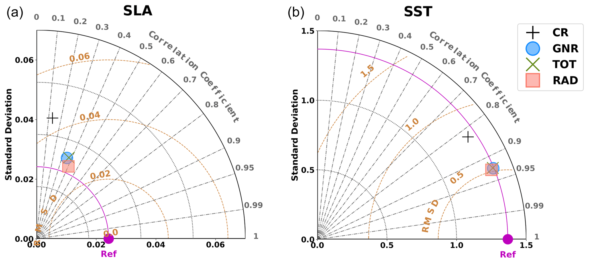
Figure 4 Taylor diagrams comparing models and observations in terms of SLA (a) and SST (b) over the whole modelling domain. The X and Y axes represent the standard deviations of the data. The distance from the reference point located on the X axis (noted as Ref in magenta) represents the centred root mean square deviation (CRMSD). Correlation between observations and the model increases clockwise. Symbols represent the different simulations, as specified in the legend

Similar conclusions are obtained when examining the Taylor diagrams focusing on Argo temperature and salinity profiles (Fig. 5). Although the CR simulation shows a very high correlation with observations (0.88 and 0.95 for temperature and salinity, respectively), this correlation is further increased for the experiments with DA. A CRMSD reduction of more than 35 % is obtained for both salinity and temperature observations in all data assimilative experiments. The diagram for the salinity shows a decrease in the standard deviation with DA and slight differences between RAD and the other two simulations.

The impact of the assimilation on the different fields was also evaluated considering only observations surrounding the IC area, leading to similar results.

Figure 5 Same as Fig. 4 for the Argo salinity (a) and temperature (b) profiles.

3.2 Eulerian assessment of the impact of DA on surface currents

To evaluate the DA capabilities to improve the representation of surface currents, we performed an Eulerian analysis in the HFR coverage area. WMOP surface daily mean velocities are compared against HFR total daily mean fields. The total observations are derived from the radial data, as described in Sect. 2.1. We compute the daily mean field only at those points that provide more than 50 % of hourly data and then interpolate the model to HFR observation grid points. As for the SLA, SST, and Argo T–S profiles, the validation can not be considered fully independent since we use the same observing platform. However, the data used for validation at a given time have not yet been assimilated in the model.

We first analyse the performance in terms of surface currents by using the Taylor diagrams for the velocity components (Fig. 6). The zonal velocity component experiences a strong correction with the assimilation of GO. Specifically, the CRMSD is reduced by 28 % while the correlation increases from 0.28 to 0.44. This performance is further improved by the two experiments using HFR data, with more than a 40 % reduction in CRMSD. While the TOT experiment exhibits the largest error reduction, RAD provides the best correlation with observations (0.7), compared to 0.63 obtained by TOT.

Considering the meridional velocity component, GNR has a lower correlation and higher CRMSD than the CR. Here, the use of HFR observations is necessary to reduce the difference between model and observations. The correlation slightly increases with the assimilation of HFR, with the best results obtained for TOT (0.47). Moreover, the standard deviation and CRMSD displays a significant reduction (27 % for TOT and 19 % for RAD).

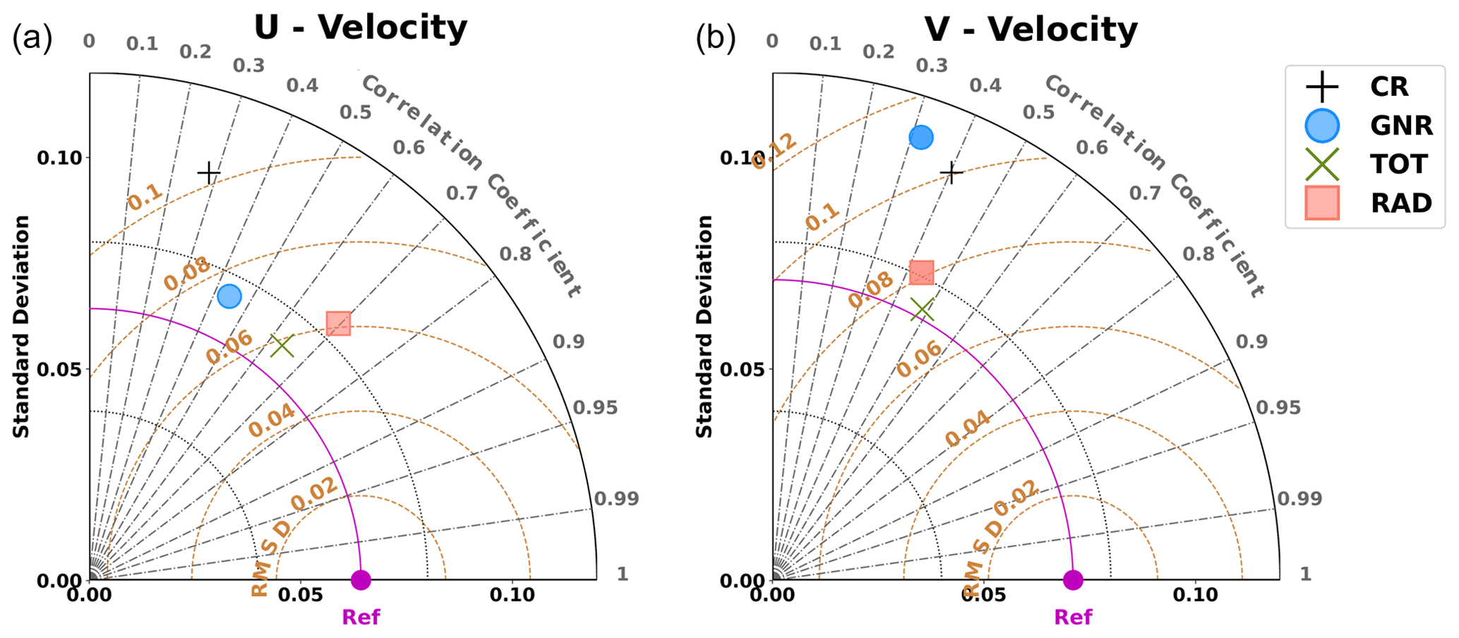
Figure 6 Taylor diagrams for WMOP simulations compared to HFR surface currents observations. Separate diagrams for each velocity component: U (a) and V (b). The symbols represent the different simulations, as specified in the legend.

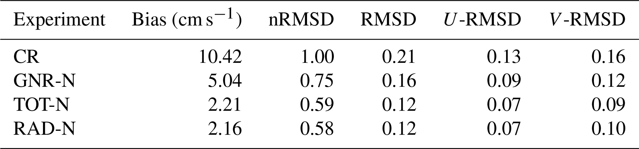
Figure 7 shows the spatial distribution of the surface current speed mean error (bias), defined as the difference between the HFR and the model in terms of the module of the velocities, at each grid point. Positive error reflects that observation mean values are larger than model estimates. The control run, CR, overestimates the currents in most of the domain with the exception of a small area on the western side. The mean bias over the whole HFR domain is 10.4 cm⁻¹ s⁻¹ (see Table 2). DA corrects the bias in all three experiments. The assimilation of GO leads to a reduction of the error over the whole domain, with a mean value of 5.4 cm⁻¹ s⁻¹. A further reduction is achieved when assimilating HFR velocities. RAD has a mean bias of 2.6 cm⁻¹ s⁻¹, which is particularly higher near the Ibiza antenna, while TOT has the lowest bias, with a mean value of 1.2 cm⁻¹ s⁻¹.

Table 2 Bias, normalized RMSD, and total RMSD between the model and HFR surface currents speed. The two columns on the right correspond to the RMSD for the zonal and meridional components.

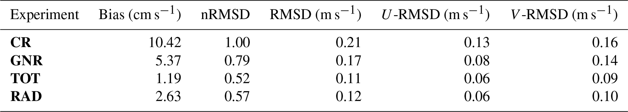
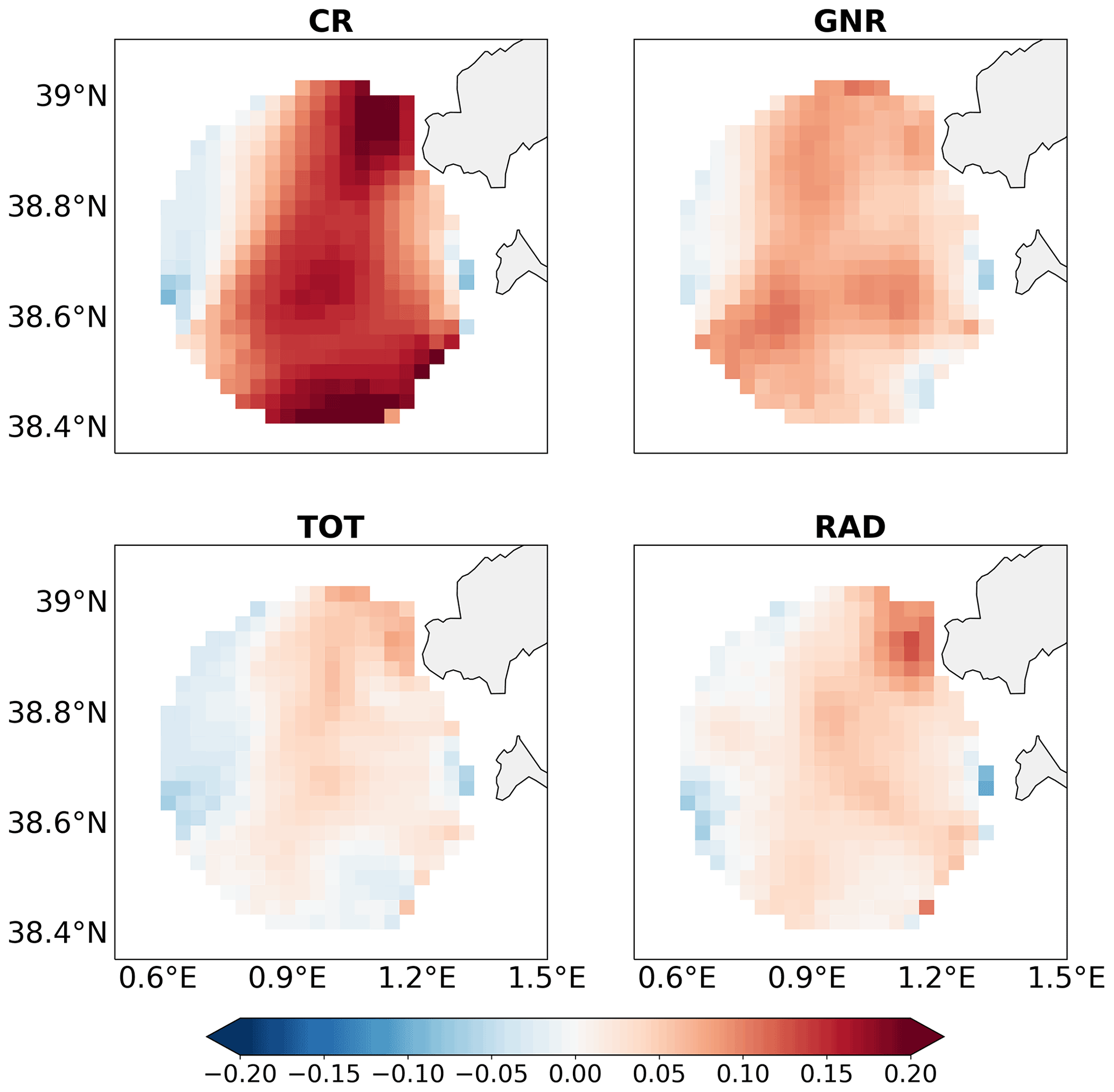
Figure 7 Mean total current speed error (bias, m s⁻¹). The mean model speed is subtracted from observations at each grid point. Positive values indicate that the model overestimates the observations on average.

3.3 Lagrangian assessment of the impact of DA on surface currents

As previously stated, 13 surface drifters were deployed in the HFR coverage area during the simulated period, as described in Lana et al. (2016). Three different kinds of surface drifters (ODi, MDOi, and CODEi) were employed, all drifting at a depth between the surface and 1 m. No significant wind drag is expected for these drifters (more details can be found in Révelard et al., 2021 or Barth et al., 2021a). Virtual particle drifts were then computed using model surface currents. For each experiment, and for eight consecutive days (from 1 to 8 October), 1000 neutrally buoyant particles were launched at each of the positions of the 13 drifters at 00:00 each day. Lagrangian tracks were simulated using OceanParcels (Lange and Van Sebille, 2017) and a 5 d period for WMOP velocity fields (at 3 h resolution). Additionally, we included a diffusion term using a Brownian motion scheme with the objective of representing the impact of the subgrid processes not resolved by the model. After each advection step the diffusion is imposed using a random distribution with a diffusion coefficient of 50 m² s⁻¹, in line with recent Lagrangian studies using the WMOP model (Cabanellas-Reboredo et al., 2019; Compa et al., 2020; Kersting et al., 2020; Torrado et al., 2021). We have verified that our results are not significantly affected by this value of the diffusion coefficient, which has a significant impact on the spread of the trajectories but not on the path of the mean trajectory.

The distance between real drifters and the centre of mass of each set of the 1000 Lagrangian particles is computed at each time step and a skill score (SS, Eqs. 4 and 5) is given for each drifter every day following the description made by Liu and Weisberg (2011). A non-dimensional index s is calculated based on the normalized cumulative Lagrangian separation distance, from purely Lagrangian parameters (Eq. 4), where d_i is the separation distance between the modelled and observed endpoints of the Lagrangian trajectory at time step i after initialization, l_oi is the length of the observed trajectory, and N is the total number of time steps.

$$\begin{array}{}\text{(4)}& {\displaystyle }s=\sum _{i=\mathrm{1}}^N{d}_i/\sum _{i=\mathrm{1}}^N{l}_{oi}\text{(5)}& {\displaystyle }\mathrm{SS}=\mathrm{1}-s\end{array}$$

Trajectories are also simulated using the hourly DIVAnd reconstructed velocity fields presented in Barth et al. (2021a). DIVAnd is a n-dimensional variational analysis method that is used here to reconstruct hourly two-dimensional vectorial fields from radial observations. It was shown to improve the reconstruction compared to the open-boundary modal analysis (Kaplan and Lekien, 2007). Figure 8 provides a few examples illustrating the Lagrangian prediction capacity for the different simulations. Each panel shows the trajectories of the drifter and the centre of mass of the virtual particles for each experiment for 48 h of simulation. These plots illustrate the diversity of situations associated with the spatio-temporal variability of the surface ocean velocities. Particularly for Panels (b), (c), (d), and (e), TOT displays very good agreement with the observations, resulting in the best performance over all the simulations. However, it is worth noting that this behaviour is not systematic and the simulations assimilating HFR sometimes fail in providing the best trajectories (Panels a and f).

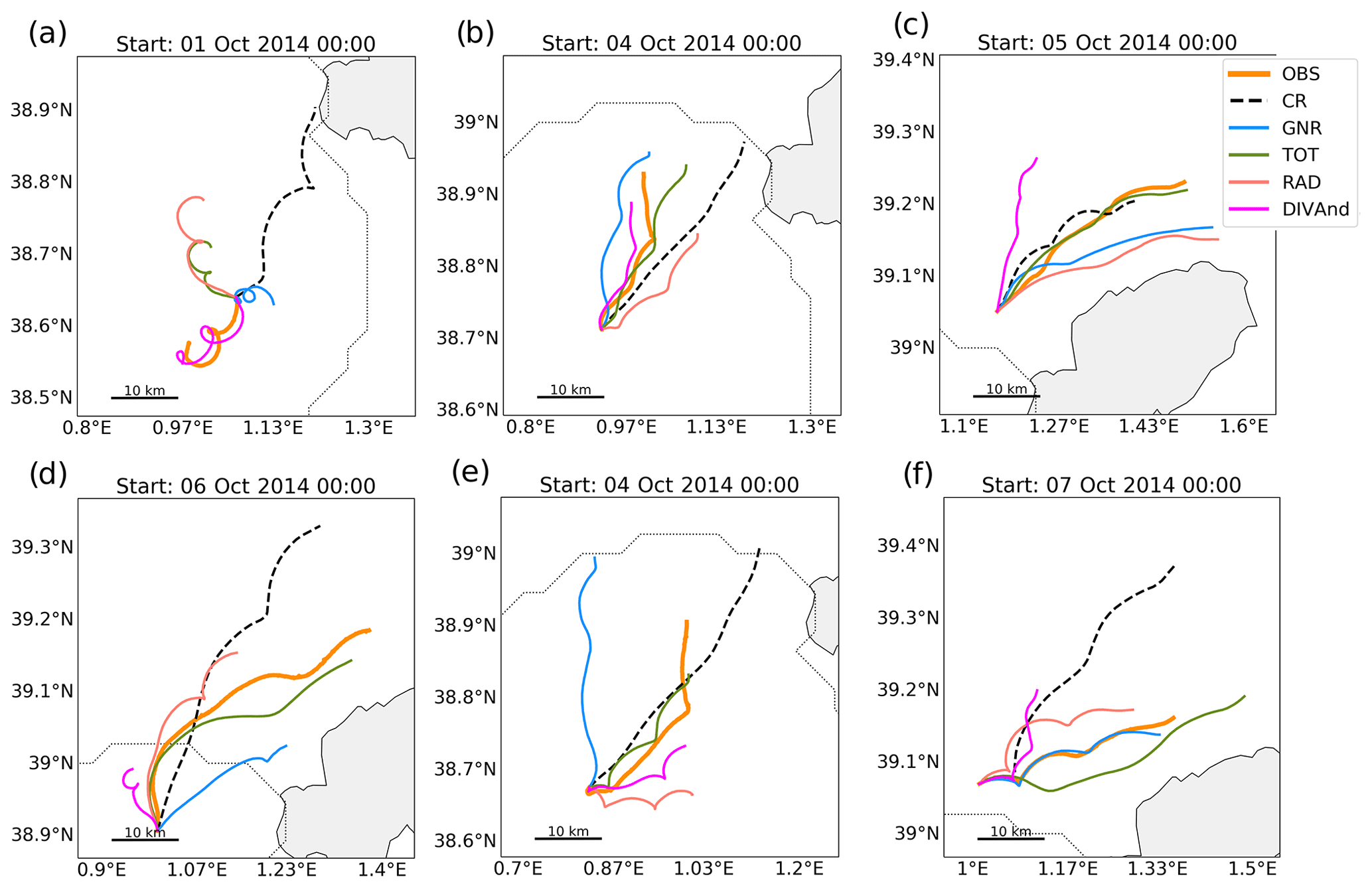
Figure 8 Map showing two-day satellite-tracked drifters and model trajectories derived from different DA experiments for different dates. Model trajectories represent the trajectories of the centre of mass of the 1000 particles launched at the drifter position at 00:00 of the indicated starting day.

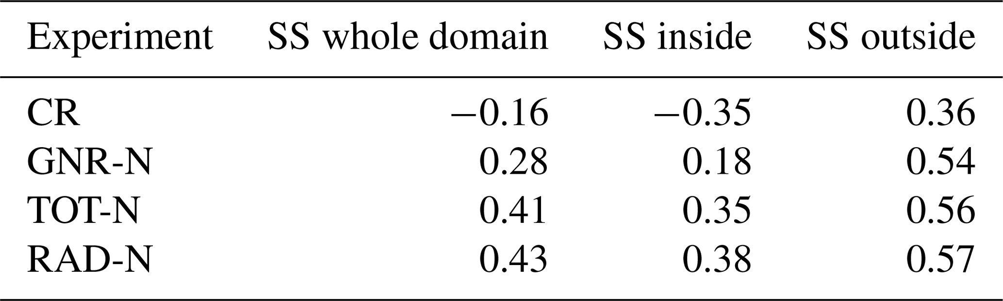
Figure 9 shows the skill score for all experiments (four model simulations + DIVAnd fields) for a forecast horizon of 48 h. Each point is located at the initial position of the particles at the beginning of the Lagrangian simulations and represents the value of the skill score of the centre of mass of the cloud of virtual particles. For trajectories with a cumulative separation distance larger than the cumulative distance travelled by the particles, the model has a negative skill score. On the other hand, values close to 1 indicate a nearly perfect match between the drifter and virtual trajectories. Values of the mean skill score are given in Table 3, where the mean skill score is computed separately for (i) all trajectories, (ii) the trajectories starting inside the HFR coverage area, and (iii) trajectories whose initial position is outside the HFR area. The top left panel of Fig. 9 shows the spatial distribution of the SS for the CR.

Inside the HFR coverage area the model has no skill for multiple trajectories (SS<0) according to Liu and Weisberg (2011), resulting in a negative mean value (−0.35). Outside there are several trajectories for which the model has some skill (SS over 0.5) and a mean value of 0.36. All experiments present a larger SS outside the HFR coverage area. This in mainly due to the characteristics of the trajectories north of the island of Ibiza, where the circulation is dominated by the Balearic current with a more steady north-eastward flow generally better reproduced in the model, as previously described by Révelard et al. (2021).

Table 3 Average skill score for the different experiments, over the whole domain, and inside and outside the HFR coverage area.

In general, all experiments with DA improve the trajectories. In particular, GNR increases the skill score compared to CR with values increasing from −0.16 to 0.19 over the whole domain. Note, however, that inside the coverage area not all trajectories are properly represented by the model (Fig. 9). The assimilation of HFR data along with GO further increases the skill score. The improvement is particularly significant inside the HFR domain, where most of the trajectories have positive SS. TOT has the best results among the model experiments, with a mean value of 0.41 inside the coverage area, which is better than RAD (0.36). Outside the coverage area all data assimilative simulations lead to a similar performance (SS around 0.58), representing an improvement with respect to CR (SS =0.36). Assimilating HFR data does not lead to any significant improvement nor degradation of the model performance outside this coverage area with respect to GNR.

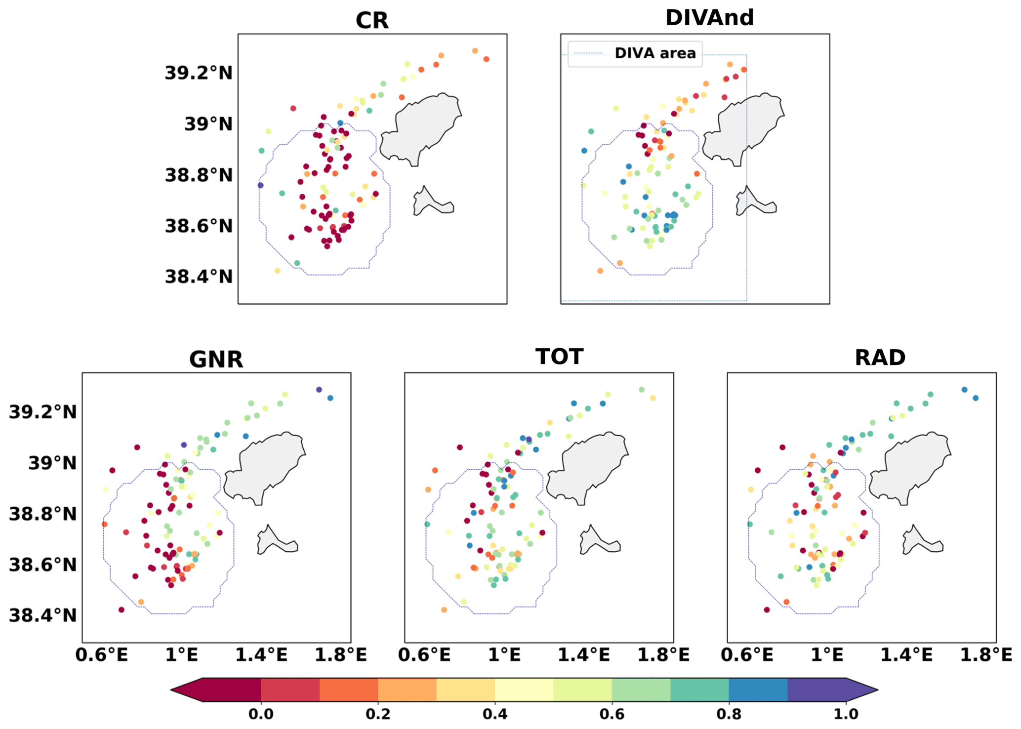
Figure 9 Scattered dots represent the skill score (Liu and Weisberg, 2011) of each simulation to represent a drifter trajectory. The dot position is the starting point of each Lagrangian simulation. Values lower than 0 mean the simulation has no skill at representing that specific drifter trajectory according to the metric used, while values close to 1 mean a perfect performance of the model. Skill score was calculated for 48 h.

The average separation distance is computed according to Eq. (6), where n_drif=13 is the number of drifters, n_part=1000 is the number of particles, and x^d and x^v are the positions of the real drifter and the corresponding virtual particle, respectively (Fig. 10). For each 5 d trajectory, the mean separation distance is first computed averaging over the number of drifters, providing a single distance as a function of time d(t) for the 13 drifters (Eq. 6). Then, the four values of d(t), one for each of the four simulations starting in consecutive days are averaged.

$$\begin{array}{}\text{(6)}& \mathrm{d}\left(t\right)={\displaystyle \frac{\mathrm{1}}{n_{\mathrm{drif}}}}\sum _{i=\mathrm{1}}^{n_{\mathrm{drif}}}\left(\left|x{{}_i}^{\mathrm{d}}\left(t\right)-{\displaystyle \frac{\mathrm{1}}{n_{\mathrm{part}}}}\sum _{j=\mathrm{1}}^{n_{\mathrm{part}}}x{{}_{ij}}^{\mathrm{v}}\left(t\right)\right|\right)\end{array}$$

The mean distance between virtual and real drifters is significantly reduced when DA is applied. The assimilation of GO efficiently helps to reduce the mean separation distance, with a reduction of 31 % after 48 h compared to CR (18.9 versus 27.2 km). Consistent with the previous analysis, the assimilation of HFR total observations along with the GO further increases the performance, leading to the lowest mean separation distance (12.8 km) with a 53 % reduction compared to the CR. The use of radial observations also leads to a high reduction of the mean separation distance (48 %), which is reduced to 14.3 km after 48 h.

DIVAnd simulations present a mean distance of 8.4 and 17.3 km after 24 and 48 h, respectively, affected by a significant number of trajectories outside of the HFR coverage area and so not properly constrained by the reconstruction algorithm.

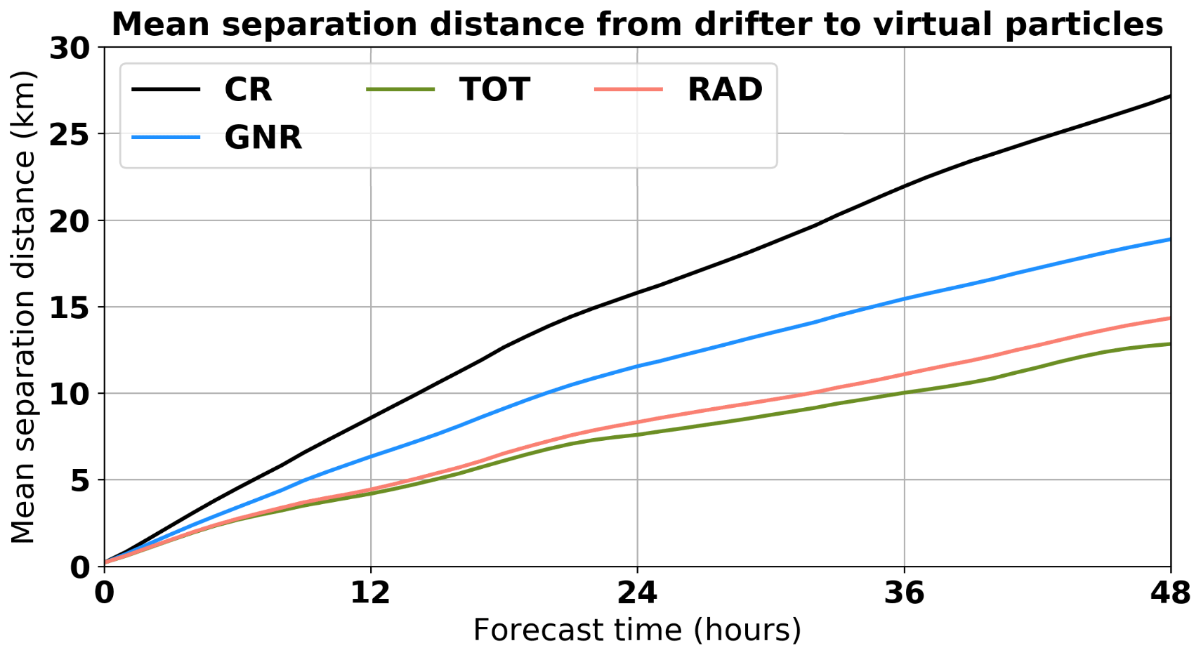
Figure 10 Mean separation distance between drifter and the centre of mass of virtual particles using the direct restart from analysis.

3.4 Impact of the nudging restart strategy

Overall, the results in the whole domain compared to satellite and Argo observations are similar to those obtained for the simulations restarting directly from the analysis. The improvement is slightly lower due to the nudging step but all data assimilative simulations provide comparable metrics. The reduction of the RMSD compared to the CR is around 8 % for the SLA, while for the SST it is reduced around 30 %. Considering Argo profiles, the reduction of the RMSD is 35 % for all simulations, both for temperature and salinity.

Table 4 presents the bias and RMSD for the model surface current speed and the zonal and meridional components. This has to be compared with Table 2, which shows the results for the simulations restarting from the analysis. We can observe a slight improvement for the GNR-N simulation when using the nudging initialization in comparison with restarting directly from the analysis, with a reduction of both the bias and the RMSD. While this initialization method also helps to reduce the bias compared to direct restart from the analysis for RAD, this is not the case when using total observations.

Table 4 Same as Table 2 for the simulations applying a nudging towards the analysis.

The Lagrangian assessment confirms these results, reflecting the usefulness of HFR data to correct surface currents using this initialization method even when the nudging is only performed towards the SSH and T–S fields. The SS for the GNR-N simulation (Table 5) increases significantly inside the coverage area while decreasing outside, with an average value of 0.39, which is larger than the value of 0.34 obtained with the other approach. The correction obtained using HFR total velocities together with GO is slightly degraded using the nudging approach both inside and outside the coverage area, with an average SS of 0.41 compared to 0.45 with the direct restart from analysis. On the other hand, RAD has a better SS when using the nudging approach. The average SS inside the radar domain increases from 0.36 to 0.38, while outside the domain it slightly decreases from 0.59 to 0.57.

Table 5 Same as Table 3 for the simulations applying a nudging towards the analysis.

The mean separation distance after 48 h when assimilating GO is also reduced from 18.9 to 16.7 km when using the nudging initialization. Although the assimilation of total HFR velocities further decreases the mean separation distance, results are slightly degraded when using the nudging compared to restarting directly from the analysis, with a mean distance of 14.0 km after 48 h. On the contrary, the assimilation of HFR radials benefits from the nudging approach, reducing the mean separation distance from 14.3 to 13.4 km after the first two days compared to the direct restart from analysis (which represents a 51 % reduction in comparison to CR) and giving the best results among all simulations using this initialization method.

4 Discussion

The assimilation of high-resolution HFR surface current observations in a reduced part of the modelling domain could have a negative effect on the rest of the variables under the effect of spurious model error correlations. While in Stanev et al. (2015, 2016) the positive outcome of the data assimilation extends beyond the HFR covered area, Zhang et al. (2010) showed that the assimilation of HFR led to an improvement of surface currents in their experiments but with a degradation of the sub-surface temperature forecasts. Sperrevik and Christensen (2015) evidenced that using T–S profiles along with HFR observations led to better results, as they control the density fields while adding a constraint on the circulation. Here we show that the assimilation of local HFR (both totals and radials) observations along with the generic ones does not degrade the improvement on the SLA, SST fields, and Argo T–S profiles achieved over the whole domain when assimilating only the generic observations. The results obtained for all experiments with DA show similar performance in this sense. Differences mostly depend on the type of initialization employed. Nevertheless, this work is mainly focused on the study of surface currents and thus the impact on sub-surface fields has not been deeply analysed. CTD casts or glider data in the region should help to complete the assessment in future studies.

We have used DIVAnd reconstructed fields as a benchmark for our Lagrangian validation. These hourly fields properly represent the inertial oscillations compared to other gap-filling techniques (Barth et al., 2021a), and we consider it as the best possible high resolution representation of the surface currents in the area, which allows the simulation of Lagrangian trajectories. It is very positive that the skill scores obtained for the HFR DA experiments are very close to that obtained by DIVAnd. While DIVAnd outperforms the capabilities of the WMOP DA system inside the coverage of both HFR antennas, it is the opposite outside this region, which demonstrates the capacity of the model to improve the representation of the currents beyond the HFR coverage area. The assimilation of GO, in particular SLA, constrains the geostrophic circulation, leading to a better representation of the Balearic current and an increase of the SS in that area. The importance of this constraint is highlighted when comparing it to DIVAnd-derived trajectories, which do not properly represent these features. While the mean SS for the DIVAnd-derived trajectories inside the area is 0.53, it drops to 0.29 outside of it, being significantly lower than all model-derived trajectories. This behaviour is consistent with the results of Barth et al. (2021a), which show that the DIVAnd reconstructed fields outside the area covered by both HFR antennas are much less reliable. Our results demonstrate the utility of dynamical models assimilating high-resolution observations as good alternatives to data-driven short-term forecasting methods, due to their capacity to extend the correction beyond the observation coverage area. They also show the importance of combining HFR and altimeter observations, which help to constrain the geostrophic circulation over a wider area.

Two different initialization strategies have been evaluated. While restarting directly from the analysis may introduce some high-frequency and spurious waves or instabilities in the system due to inconsistencies between the corrected fields and the model equations, it considers an initial state that is closer to observations. On the other hand, the nudging strategy provides a more conservative framework in which the model dynamics are better respected but with the drawback that some of the correction achieved with the observations may be lost. Overall, both approaches show similar results leading to a reduction of the RMSD over the whole domain. As in the case of the direct restart from the analysis, the use of the “nudging” strategy also leads to an improvement of the predictions of surface currents when assimilating HFR observations compared to the simulation that only uses generic data sources. It is important to point out that, in our case, nudging is only applied towards the temperature, salinity, and sea surface height fields, but not towards the velocity fields, to avoid model instabilities. Therefore, the assimilation of the surface currents enables us to correct the density fields, which in turn improves the surface velocities due to the model initial adjustments.

The nudging strategy limits the possible shocks and anomalous gradients that may be generated in the analysis so that the solution remains closer to the physical balances. We found that it was not optimal for surface currents prediction when using HFR total velocities but a better choice for radial data. This is probably due to the fact that reconstructed total velocities are already smoothed out through a pre-processing step contrarily to the case of radial data, which are more noisy and directly benefit from the smoothing effect of the nudging approach. The nudging strategy appears to be a good solution for operational purposes when the occurrence of noisy data tends to be more frequent. It may also be a good choice for systems depending on operational data sources for which HFR antennas, for instance, may not work during certain periods or satellite and Argo data may not be available on time. It could also be less sensitive to potential errors in data in cases where near real-time observations could be affected by significant errors.

The observation error was considered the same for total and radial currents in this study, as explained in Sect. 2.3, without considering any spatial variability. Some authors used spatially variable observation errors depending on whether the area is covered by a single antenna or more than one (Vandenbulcke et al., 2017). Here we have considered the same error for all HFR radial observations so as to also exploit the potential benefit of observations in areas covered by only one antenna, as discussed in Shulman and Paduan (2009); Stanev et al. (2015). However, the evaluation of the effect of penalizing observations with larger errors in areas covered by a single antenna or affected by geometry dilution of precision (GDOP) effects is relevant and would need further research. The observation error should also ideally include correlated observation errors, even if our knowledge of these errors is still somehow limited. This is another interesting aspect that should be evaluated in future studies.

5 Conclusions

In this work, we have integrated different multivariate ocean observations with numerical modelling to improve the dynamical knowledge of ocean currents in line with the actual concerns in operational oceanography (De Mey-Frémaux et al., 2019; Kourafalou et al., 2015a, b; Schiller et al., 2015). This work has benefitted from the collaborative framework of the JERICO-NEXT European research infrastructure initiative (Farcy et al., 2019), which aims at fostering cooperation to build a sustained coastal observing network. We combined high-resolution modelling with satellite and in situ observing sources and HFR surface currents measurements to discuss the contribution that the developing HFR networks could provide to regional and coastal operational modelling. The impact of HFR-DA was evaluated using both radial and total observations along with generic data sources as SLA, SST, and Argo T–S profiles. The system showed its ability to improve the representation of ocean fields by assimilating different types of observations from a variety of sources observing a wide range of spatio-temporal scales.

The assimilation of generic observation sources helps to correct surface currents in the IC as revealed by both the Eulerian and Lagrangian validations. The employment of HFR observations further improves the forecasting of surface currents in the IC. While GNR simulations reduce the RMSD and the mean error, the assimilation of HFR leads to an increase in the correlation between model and observations for both components of the velocity. The Lagrangian validation reveals the capacity of HFR data assimilation to improve the prediction of surface currents inside the area covered by both antennas, while not degrading the representation of the more steady currents found outside of it. The experiment assimilating HFR total velocities is the one that best fits the observations. In addition, it provides the best average skill score for Lagrangian prediction and the lowest mean separation distance between drifters and virtual particles. The use of radial observations benefits from the use of an intermediate nudging initialization approach after the analysis. The results presented in this study confirm the usefulness of HFR systems to improve regional operational ocean forecasting models, even when providing limited coverage with respect to the model domain extension.