the Creative Commons Attribution 4.0 License.
the Creative Commons Attribution 4.0 License.
 | 12 Nov 2020
Extreme waves and climatic patterns of variability in the eastern North Atlantic and Mediterranean basins
Verónica Morales-Márquez
Alejandro Orfila
Gonzalo Simarro
Marta Marcos
The spatial and temporal variability of extreme wave climate in the North Atlantic Ocean and the Mediterranean Sea is assessed using a 31-year wave model hindcast. Seasonality accounts for 50 % of the extreme wave height variability in the North Atlantic Ocean and up to 70 % in some areas of the Mediterranean Sea. Once seasonality is filtered out, the North Atlantic Oscillation and the Scandinavian index are the dominant large-scale atmospheric patterns that control the interannual variability of extreme waves during winters in the North Atlantic Ocean; to a lesser extent, the East Atlantic Oscillation also modulates extreme waves in the central part of the basin. In the Mediterranean Sea, the dominant modes are the East Atlantic and East Atlantic–Western Russia modes, which act strongly during their negative phases. A new methodology for analyzing the atmospheric signature associated with extreme waves is proposed. The method obtains the composites of significant wave height (SWH), mean sea level pressure (MSLP), and 10 m height wind velocity (U10) using the instant when specific climatic indices have a stronger correlation with extreme waves.
- Article
(31075 KB) - Full-text XML
- BibTeX
- EndNote


The accurate assessment of extreme wind-wave conditions is essential for human activities, e.g., maritime traffic and wave energy generation, and is a major source of coastal hazards. Extreme waves influence the upper ocean by enhancing vertical mixing through the Stokes layer (Polton et al., 2005). Extreme waves reaching port areas also determine the design and operation of coastal and offshore infrastructures; they are also responsible for coastal flooding at intra-annual scales (Orejarena-Rondón et al., 2019). Waves are the ocean surface response to the wind stress acting over it, and therefore there is a direct connection between surface atmospheric circulation and waves (Lin et al., 2019).
The study of extreme waves at different temporal scales has been extensively addressed in several works (Wang and Swail, 2001, 2002; Caires et al., 2006; Méndez et al., 2006; Menéndez et al., 2008, 2009; Izaguirre et al., 2010, 2012; Young et al., 2012; Weiss et al., 2014; Sartini et al., 2017). Most of these studies focused on the spatiotemporal distribution of extreme waves rather than on the atmospheric conditions producing them.
Over the North Atlantic Ocean and the Mediterranean Sea, atmospheric circulation is driven by the temperature gradient between the North Pole and the Equator that organizes a three-cell system associated with the equatorial low, the subtropical Azores High, the Icelandic Low, and the North Pole high-pressure center (Martínez-Asensio et al., 2016). Atmospheric circulation can be characterized by specific modes of variability with defined characteristics that may also have effects over a region or remote area through atmospheric teleconnections (Wallace and Gutzler, 1981). The main patterns of atmospheric variability in the North Atlantic and Europe are the North Atlantic Oscillation (NAO), the East Atlantic (EA) pattern, the Scandinavian pattern (SCAND), and the East Atlantic–Western Russia (EA/WR) pattern (Barnston and Livezey, 1987). NAO is the leading mode of variability in the North Atlantic and is often defined as the sea level pressure difference between the Icelandic Low and the Azores High (Hurrell et al., 2003). NAO controls the strength and direction of westerly winds reaching European coasts and the location of the storm tracks across the North Atlantic (Marshall et al., 2001). The EA is the second predominant mode of low-frequency variability in the North Atlantic area. It consists of a north-south dipole of anomaly over the North Atlantic, with a strong multidecadal variability. The SCAND pattern consists of a primary circulation center over Scandinavia, with weaker centers of opposite sign over western Europe. The EA/WR pattern consists of four main anomaly centers; its positive phase is associated with positive wave height anomalies located over Europe and negative wave height anomalies over the central North Atlantic (https://www.cpc.ncep.noaa.gov/data/teledoc/telecontents.shtml, last access: 27 February 2020).
There have been a number of studies that have tried to unravel the relation between wave climate and large-scale atmospheric patterns. Woolf et al. (2002) found a strong connection between interannual wave climate variability in the North Atlantic Ocean and the NAO, as well as with the EA index to a lesser degree. Castelle et al. (2018) examined the relation between winter mean wave height, detailing a high correlation with the NAO index and with the Western Europe Pressure Anomaly (WEPA) index; this is a new definition of a climatic pattern based on the sea level pressure gradient between the stations Valentia (Ireland) and Santa Cruz de Tenerife (Canary Islands). Izaguirre et al. (2010) detected a relation between the NAO and EA indices with the extreme wave climate in the northeast Atlantic Ocean. Izaguirre et al. (2012) evaluated the synoptic atmospheric patterns associated with the extreme significant wave height (SWH), finding a higher interannual variability of the extreme SWH in the northern part of the Atlantic Ocean. In the Mediterranean Sea, clear relations between extreme waves and the negative phases of EA and the EA/WR indices have been also reported (Izaguirre et al., 2010).
In this paper, we extend earlier studies by analyzing the short- and long-term variability of extreme waves in the North Atlantic Ocean and in the Mediterranean Sea, not only for diagnostic purposes but also to be able to provide statistical prognostics of extremes waves associated with the most important climatic indices. The paper is structured as follows. In Sect. 2, the data used and the description of the extreme waves are presented. In Sect. 3, we present the spatial and temporal distribution of the extreme waves and the relation between the four patterns of climatic variability and the spatial distribution of extreme waves during winter. Finally, Sect. 4 concludes the work.
2.1 Waves and atmospheric data
Wave data are obtained from a high-resolution global hindcast from the National Center for Environmental Prediction (NCEP) with a temporal sampling of 1 h and different spatial resolutions. This dataset (i.e., WAVEWATCH III 30-year Hindcast Phase 2, Chawla et al., 2012) has been generated by forcing the “state-of-the-art” wave model WAVEWATCH III (Tolman, 2009) with 10 m height high-resolution wind fields from the NCEP Climate Forecast System Reanalysis and Reforecast (CFSRR), a 30-year homogeneous dataset of hourly 1∕2∘ spatial resolution winds.
The wave model consists of global and regional nested grids, developed by the presence of currents and bathymetry (Amante and Eakins, 2009), taking into account the conservation of action density (Janssen, 2008). In addition, the dissipation and physical term parameterization formulated in Ardhuin et al. (2010) is used in this work.
The hindcast has been validated using the National Data Buoy Center (NOAA NDBC) and with the altimeter database provided by the Institut Français de Recherche pour l’Exploitation de la Mer (IFREMER) (Chawla et al., 2011, 2012, 2013).
The simulation spans a time period of 31 years from 1979 to 2009 with hourly outputs, although since we assume that wave climate is constant for 3 h, we only use one data point for this period with a spatial resolution varying according to the study area. In all the grids, the full-resolution ETOPO1 bathymetry is used in regular spherical grids. The North Atlantic domain spans from 20 to 70∘ N in latitude and 60∘ W to 10∘ E in longitude at 0.5∘ resolution (Fig. 1a). The Mediterranean Sea covers 30 to 48∘ N in latitude and 7∘ W to 43∘ E in longitude with a spatial resolution of 0.167∘ (see Fig. 1b). Sea level pressure and wind velocity at 10 m of height are provided by the NCEP CFSRR forcing with a resolution of 0.5∘ for the same period (Saha, 2009).
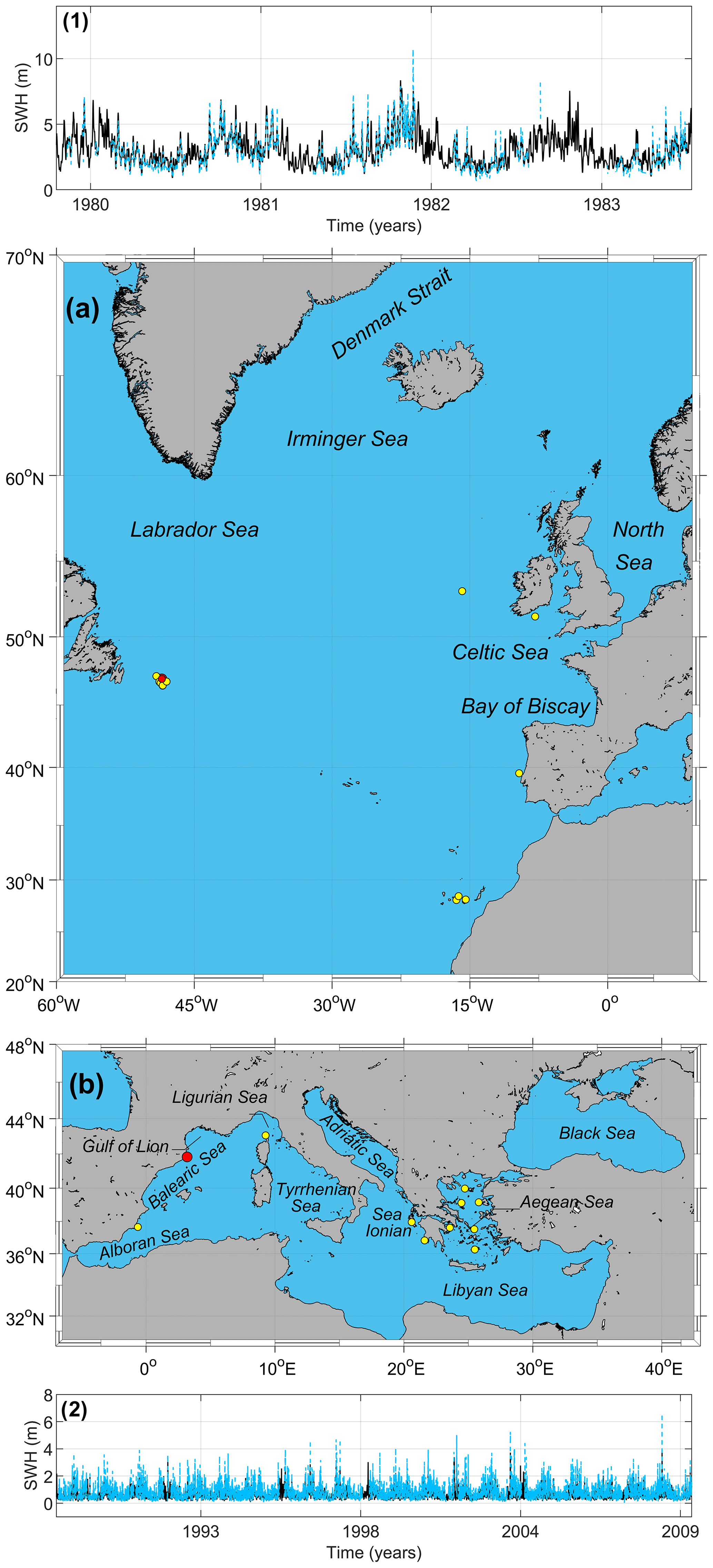
Figure 1Location of the study zones. (a) Eastern North Atlantic Ocean. (b) Mediterranean Sea. The yellow points are the locations of the buoys used in the comparison with the modeled data by WAVEWATCH III 30-year Hindcast Phase 2. Panels 1 and 2: SWH series of hindcast (black line) and a representative buoy (dashed blue line) for the North Atlantic Ocean and Mediterranean Sea, respectively. The red points are the locations of the representative buoys.
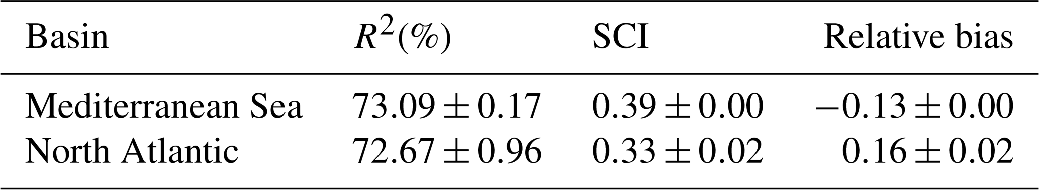
The hindcast is validated at the two basins with available buoys following the methodology described in Morales Márquez et al. (2018). For 13 buoys in the Atlantic and 11 in the Mediterranean Sea, we compute the correlation coefficient (R2), scatter index (SCI), and relative bias (RB) as
with m representing the modeled dataset by WAVEWATCH III 30-year Hindcast Phase 2 and b the in situ buoy dataset.
Table 1 shows the comparison between the WAVEWATCH III 30-year Hindcast Phase 2 and the buoys from the Copernicus Marine Environment Monitoring Service (CMEMS, https://marine.copernicus.eu/, last access: 2 July 2020). See Fig. 1 for buoy locations.
Table 1Statistical comparison between the WAVEWATCH III 30-year Hindcast Phase 2 and CMEMS buoys.
Leading climatic modes of variability, namely NAO, EA, EA/WR, and SCAND (see the Introduction for a description of these modes), have been downloaded from the NOAA Climate Prediction Center. Indices are constructed through a rotated principal component analysis of the monthly mean standardized 500 mb height anomalies in the Northern Hemisphere, ensuring independence between modes at a monthly scale due to orthogonality (Barnston and Livezey, 1987).
2.2 Extreme wave climate
Extreme wave climate is defined here in terms of the monthly 99th percentile of SWH (hereinafter SWH99). Over the North Atlantic, maximum values of SWH99 during the whole period of time analyzed (1979–2009) are observed at middle to high latitudes with values reaching 13 m (see Fig. 2a). This situation is very similar to results obtained in Vinoth and Young (2011), wherein there are higher values of SWH in the northern part of the study area. These maximum values occur predominantly during winter (DJFM), with an 81.2 % occurrence (Fig. 2c). Over the Mediterranean Sea, maximum values of SWH99 are at most 8 m (Fig. 2b), with a 91.06 % occurrence during winter (DJFM) (Fig. 2d).
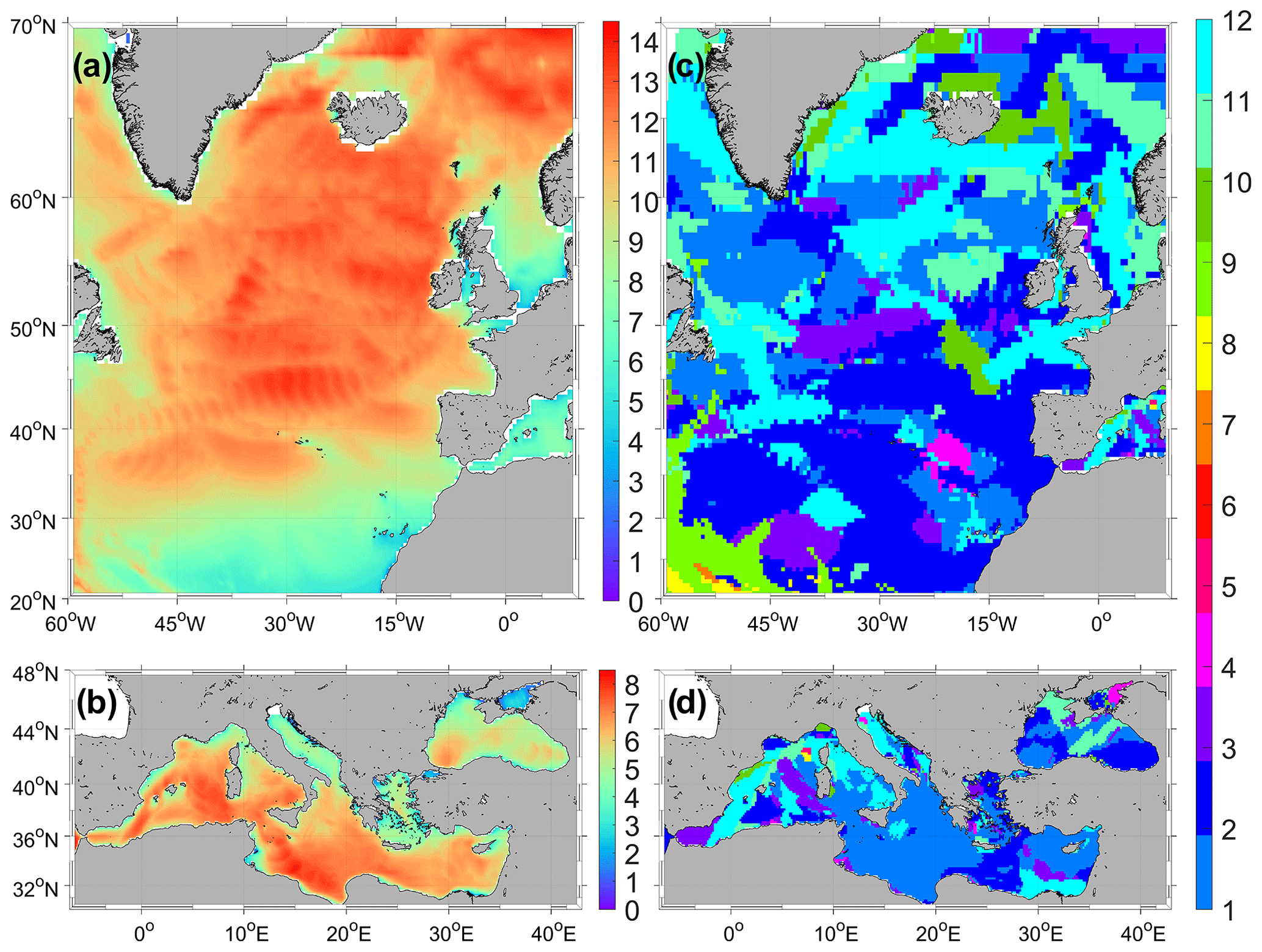
Figure 2Maximum value of monthly 99th percentile SWH in meters for (a) the North Atlantic Ocean and (b) Mediterranean Sea, as well as the month of the year (from January to December; 1: January, 2: February, and so on) when there is a maximum value of the 99th percentile SWH for (c) the North Atlantic Ocean and (d) Mediterranean Sea.
Seasonality is assessed by fitting a cosine function to the monthly SWH99 series through a least-squares adjustment (Menéndez et al., 2009):
where represents the annual and semiannual cycle, Ai the amplitude, ϕi the phase, and 182.63, and t time in days. The monthly SWH99 for the location with the largest variance reduction in the North Atlantic (point 1, Fig. 3a) is shown in black in the top panel of Fig. 3 (the same for the Mediterranean Sea, point 2 in Fig. 3b), while the time series after removing seasonality by fitting Eq. (4) are shown in blue. Seasonality in the North Atlantic accounts on average for 50 % of the variance in the signal (Fig. 3a). It means that half of the extreme wave signal is explained by the annual and semiannual cycle. In the Mediterranean Sea, there are two different areas in terms of seasonality. One is located in the central basin where seasonality explains up to 70 % of extreme waves, and the other is located in the Gulf of Genoa and the Alboran Sea, where seasonality explains less than 10 % of the signal (Fig. 3b). These areas are very active in terms of cyclogenetic activity (Trigo et al., 2002), and thus the seasonal signal is relatively less important here.

Figure 3Variance reduction in percentage if the seasonality is removed from the monthly 99th percentile SWH series for the (a) North Atlantic Ocean and (a) Mediterranean Sea. Panels 1 and 2: monthly 99th percentile SWH series (black line) and monthly 99th percentile SWH series without seasonality (blue line) for a point in the North Atlantic Ocean and Mediterranean Sea, respectively.
To analyze the long-term trend of SWH99 during winter months (DJFM) when most extreme waves occur, the temporal series is fitted by a linear regression in time at the 90 % confidence level at each spatial point (see Fig. 4). Locations where the trend is not significant are represented with a dot. The 31-year trend in the North Atlantic (Fig. 4a) displays an area with significant positive values (up to 2.5 cm yr−1) from the Portuguese coast to Canada. The rest of the basin presents a negative value tendency, with maximum values around 3.5 cm yr−1 in the Bay of Biscay, Labrador Sea, and between the United Kingdom and Iceland. This aligns with the obtained results in Gallagher et al. (2016), wherein the future projections of mean surface wind show an average decrease over the North Atlantic Ocean for winter, so the extreme waves likely continue with the same pattern in terms of long-term variability. In the Mediterranean Sea, the values of SWH99 tendency during winter months (DJFM) are substantially smaller (see Fig. 4b). Only the center part, north of Cyprus (with negative values up to 2.4 and 1 cm yr−1, respectively) and the Aegean Sea (with positive values for the trend of around 1 cm yr−1), presents a trend that is statistically significant. These calculations are restricted to the time period corresponding to the atmospheric forcing of the WAVEWATCH III 30-year Hindcast Phase 2, and different patterns could be obtained for different periods.
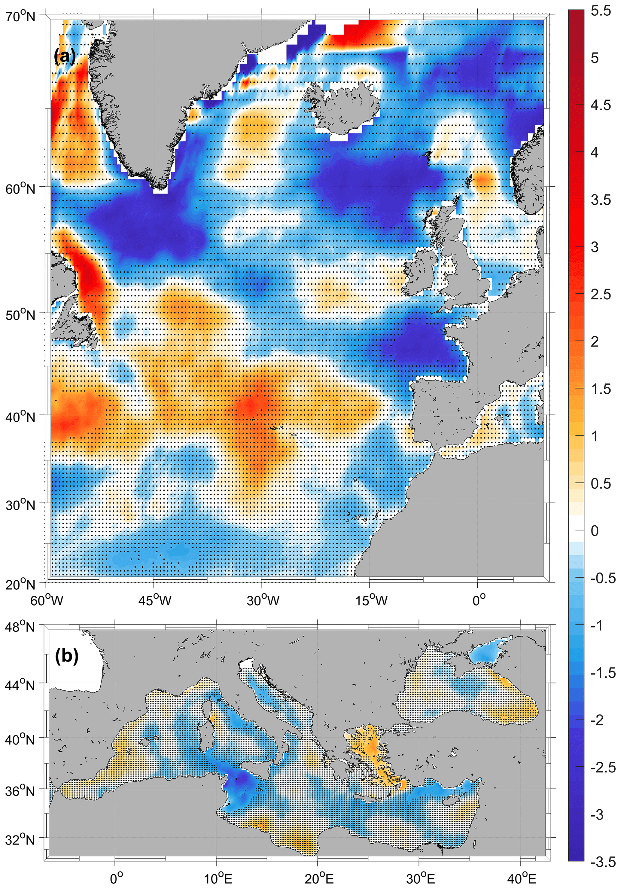
Figure 4Trend of the monthly 99th percentile SWH during winters (DJFM) in centimeters per year. Dotting indicates no significant values at the 90 % confidence interval.
These results differ from the trend calculated in Young et al. (2011), since in that study they considered all the months of the year in order to calculate the monthly SWH99 trend, and in this work, we analyze the tendency of the monthly SWH99 only during winter (DJFM). We have verified that there is a positive trend of SWH99 during the summer season (it is not shown in this study); however, the values in this season are considerably lower than those found during winters.
In this paper the winter extreme wave climate is studied in order to remove the seasonality because maximum values of SWH99 take place during the winter season.
The spatiotemporal variability of SWH99 is assessed by computing empirical orthogonal functions (EOFs) of the winter (DJFM) fields. Prior to the computation of the EOFs, the spatial mean winter SWH99 was removed and the analyses were performed on anomalies with respect to the mean values (Ponce de León et al., 2016). Mean fields are mapped in Figs. 5a and 6a.
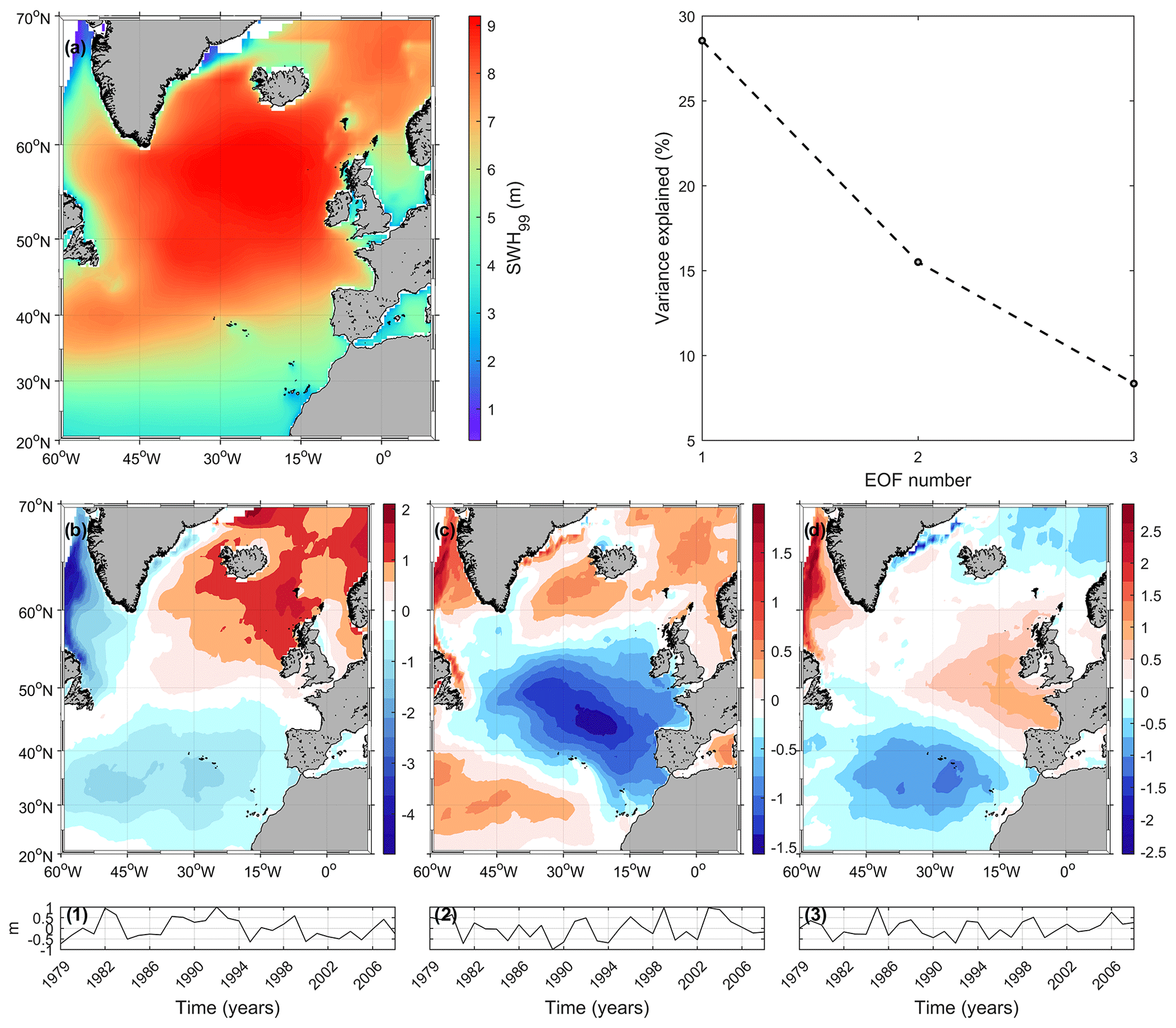
Figure 5(a) Mean field of winter SWH 99th percentile over the North Atlantic. EOF analysis of SWH99 anomalies, showing the explained variance of the first three EOFs, (b–d) spatial patterns of EOFs 1–3, and (1–3) principal components of the EOFs above.
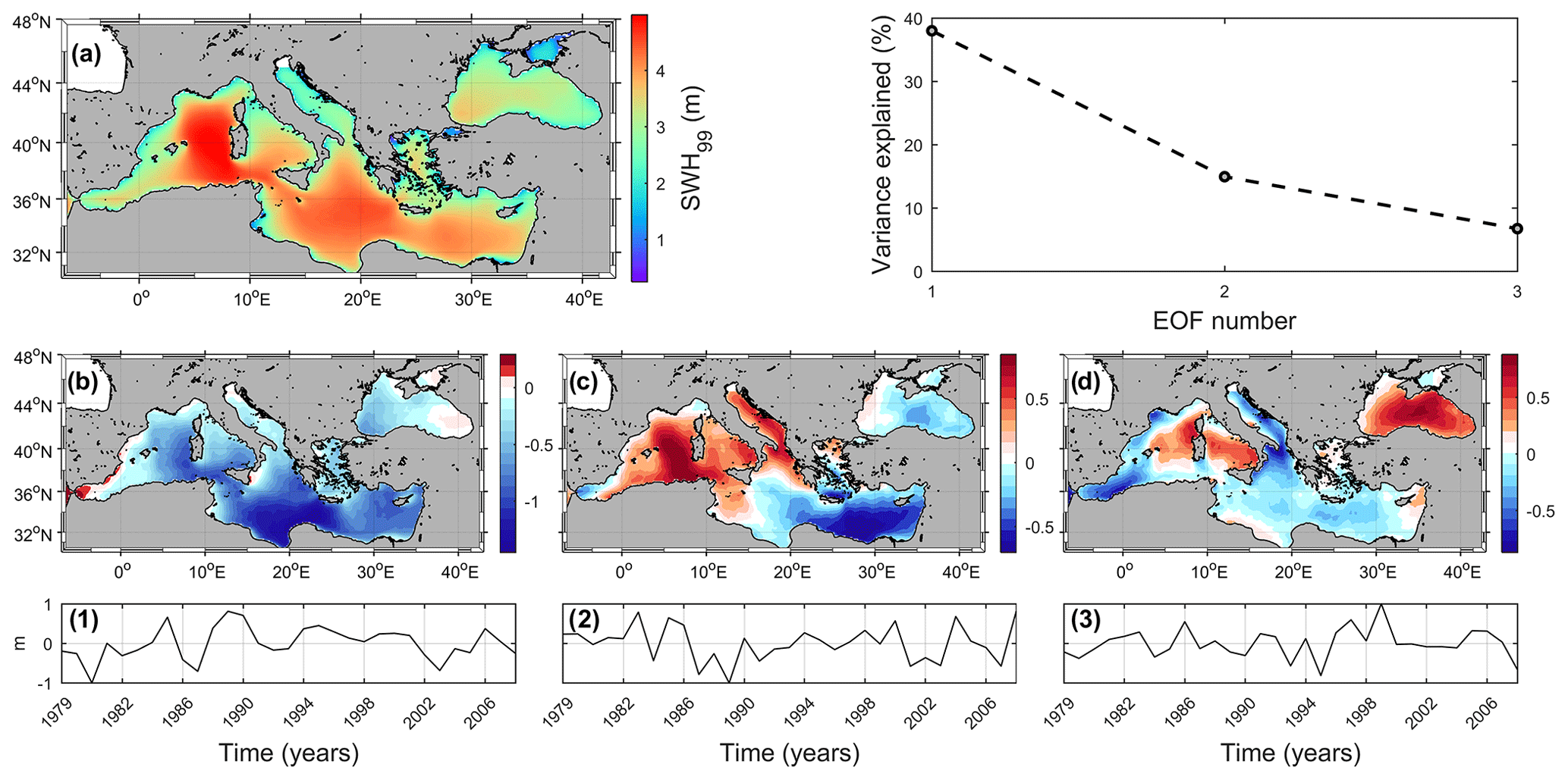
Figure 6(a) Mean field of winter SWH 99th percentile over the Mediterranean Sea. EOF analysis of SWH99 anomalies, showing the explained variance of the first three EOFs, (b–d) spatial patterns of EOFs 1–3, and (1–3) principal components of the EOFs above.
The first three EOFs for the North Atlantic are shown in Fig. 5b–d and their principal components (PCs) together with their explained variance in Fig. 5 (1, 2, and 3). The first EOF, which explains 28.5 % of the winter SWH99, presents a periodicity in its PC of around 5 years (calculated through a fast Fourier transform analysis in Fig. 5, panel 1). This first mode shows a spatial dipole with opposite values in the north and south of the basin. The second mode, which explains 15.5 % of the winter variability, shows an area in the central basin separating two zones at the north and south with different sign (Fig. 5c). Values for the central part are 3 times larger than the ones obtained for the northern and southern sides, indicating that the contribution of this EOF is to increase (decrease) the winter extremes in the central Atlantic when its PC is negative (positive). The third EOF, which explains 8.3 % of the winter variability, also displays three different zones with a central area shifted to the east-west direction extending from the Bay of Biscay to the Celtic Sea and at the north and south zones displaying an opposite sign during winter (Fig. 5d).
For the Mediterranean Sea, the first three EOF modes for winter are shown in Fig. 6b–d and their PCs in Fig. 6 (1, 2, and 3). The first EOF, explaining 38.0 % of the total variance, represents a spatially coherent increase (decrease) in SWH99 over the entire basin. The second EOF, explaining 15.1 % of the variance, shows differences between the eastern and western basins. The contribution of this mode is to increase (decrease) SWH99 in the western Mediterranean with a simultaneous decrease (increase) in the eastern Mediterranean according to the amplitude of the PC. Finally, the third EOF, explaining 7.3 % of the variance, displays two zones: the Tyrrhenian Sea and the southern part of the Gulf of Lion with the same sign and the rest of the basin with opposite behavior.
The relationship between extreme waves and the climatic modes of variability in the North Atlantic Ocean and Mediterranean Sea is explored and quantified as follows. Winter averages of climate indices are first correlated with the corresponding PCs described above for each basin. The significance level is set at 90 % with a t-value analysis adjusted as
where c the correlation coefficient and N the length of the time series. If t is equal to or higher than the t-value statistics of a Student's t distribution of N−2 degrees of freedom, then the correlation is assumed to be statistically significant at the predefined 90 % confidence level. These significance values are particular for this study since they depend on the data used and the analyzed time period.
3.1 Correlations between winter extreme waves and climatic modes of variability
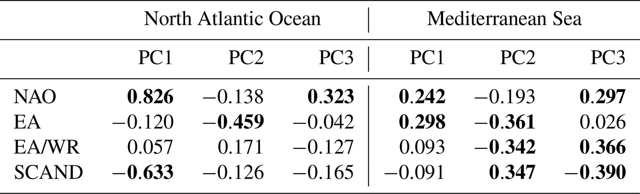
The correlation between the four climate indices and the first three SWH99 PCs are shown in Table 2 where (and hereinafter) bold indicates statistically significant correlations at the 90 % confidence level. The major correlation in the North Atlantic is obtained with the NAO and the SCAND through PC1 (correlation of 82.6 % and −63.3 %, respectively). This is not surprising, as winter NAO and SCAND indices are correlated themselves (note that, although monthly indices are orthogonal, this does not necessarily hold for seasonal or yearly averages). The NAO teleconnection not only dominates the extreme values of SWH during winter, but also the mean SWH, wave period, and peak wave direction magnitudes for wintertime in this region (Gallagher et al., 2014). To a lesser extent, EA is correlated with the second PC (explaining around 16 % of the winter variability). These results are in accordance with those obtained by Izaguirre et al. (2010) and Gleeson et al. (2019), who show that extreme waves in the North Atlantic are related to the positive phase of NAO and the negative of EA and SCAND. For the Mediterranean Sea, both the NAO and the EA are correlated with the winter SWH99 through the first PC, and some of the variability is correlated with the negative phases of EA and EA/WR through the second PC. However, the values of the correlations in the Mediterranean Sea are significantly lower than those in the North Atlantic because the main climatic patterns consist of some strong poles located in the Atlantic Ocean, which drive zonal flows toward Europe. These climatic situations generate a weak circulation into the Mediterranean Sea, which is not as related to the higher values of waves. In addition, wave climate depends on wind regimes and on land-sea distribution. In other words, waves need fetch to develop, and in the Mediterranean Sea, the available distance is more restricted (Lionello and Sanna, 2005).
Table 2Correlation between main climate indices and the amplitudes of the first three modes of the average monthly SWH99 series for the North Atlantic Ocean and Mediterranean Sea in winter.
3.1.1 Atlantic Ocean
Correlation maps for winter SWH99 in the North Atlantic and the four climate indices are displayed in Fig. 7. Some of these spatial correlations present similarities to the EOF patterns shown in Fig. 5. In particular, the correlation map between NAO and SWH99 (Fig. 7a) mimics the first SWH99 EOF for winter (Fig. 5b), with correlation values consistent with the one obtained using PC1 (see Table 2). The correlation between EA and SWH99 (Fig. 7b) shows large similarities to the second SWH99 EOF for winter extreme waves (see Fig. 5c) but with the opposite sign. Finally, the correlation between SCAND and SWH99 (Fig. 7d) shows similarities to the first SWH99 EOF (Fig. 5b). During winter, the northern part of the North Atlantic Ocean has a positive correlation with the NAO and a negative correlation at the south with maximum values close to 0.8 (Fig. 7a). The correlation map for the EA index shows positive correlations with maximum values close to 0.75 in the central part of the basin and a negative correlation at the north and south, with maximum values of 0.47 (Fig. 7b). The correlation map for the EA/WR displays an area of negative correlation extending from the Bay of Biscay to Greenland and also near the west coast of Africa. At the northern and central basin there appear to be two zones with a positive correlation, with maximum values around 0.55 (Fig. 7c). Finally, the correlation map between SCAND and SWH99 shows negative correlations in the central Atlantic, with maximum values of 0.74, and positive correlations in the central Atlantic with a maximum value of 0.60 (Fig. 7d).
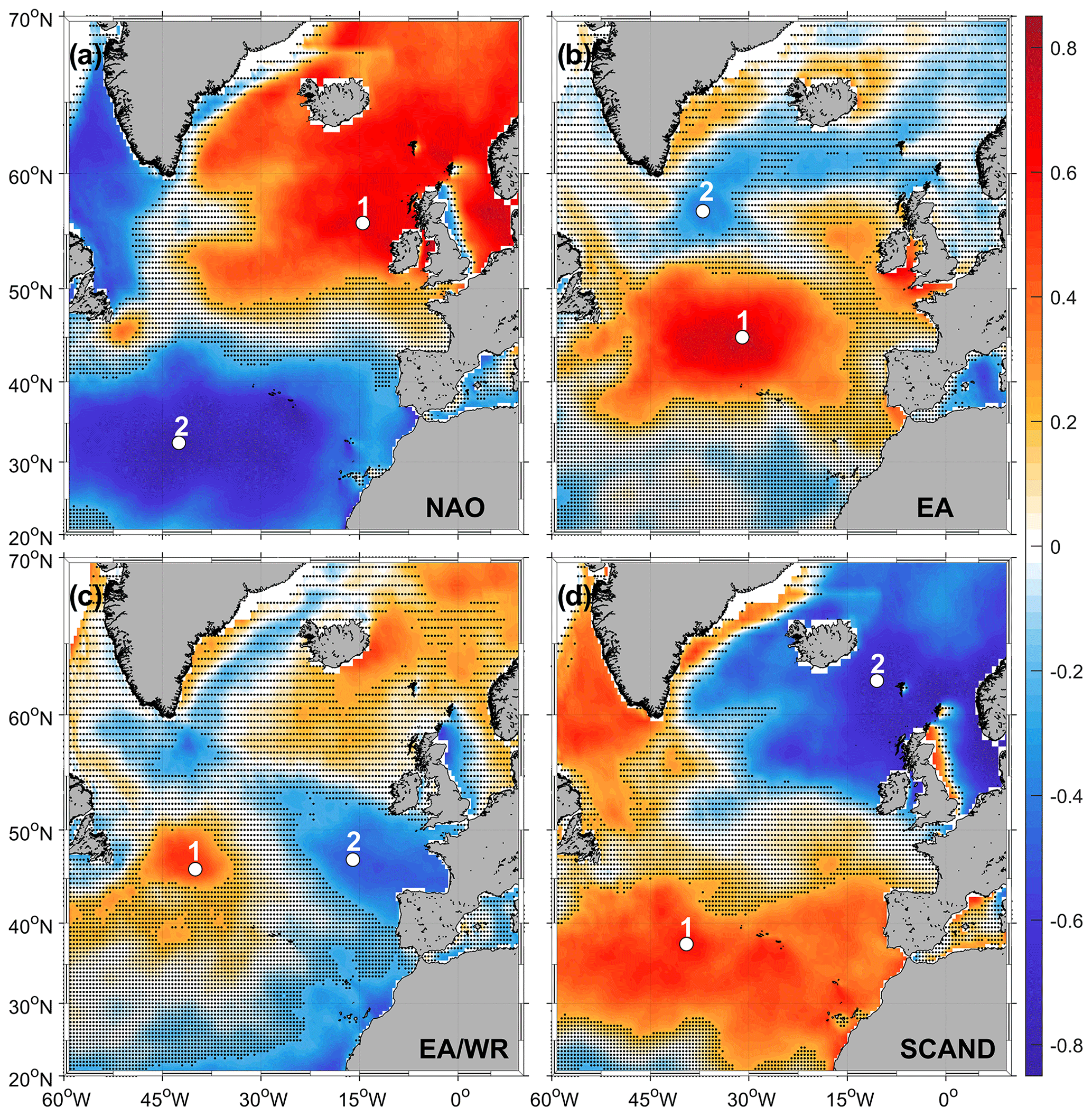
Figure 7Pearson correlation coefficient of winter mean 99th percentile SWH North Atlantic series and (a) NAO, (b) EA, (c) EA/WR, and (d) SCAND winter mean indices. Dotting indicates no significant values at the 90 % confidence interval. The white points show (1) the maximum positive and (2) the maximum negative value of the correlation coefficient.
3.1.2 Mediterranean Sea
Correlation maps between winter SWH99 in the Mediterranean Sea and the four climatic indices are shown in Fig. 8. Contrary to what is found in the North Atlantic, maps of correlations between extreme waves and climate modes are not clearly linked with the EOF patterns of the wave field. The NAO index presents a negative correlation in the whole Mediterranean basin (Fig. 8a). The eastern side of the domain, the Adriatic and Aegean Sea, presents maximum correlations with values around 0.50. The correlation is positive only in the Ligurian Sea, with a value around 0.30. The EA index also displays a negative correlation in the whole domain (Fig. 8b), with larger values over the west with a correlation around 0.60. The correlation map between EA/WR and SWH99 shows negative correlations in the Tyrrhenian Sea, the Adriatic Sea, and the Ionian Sea with a maximum correlation of 0.40 (Fig. 8c). A positive correlation is obtained in the Aegean Sea with maximum values around 0.60. Finally, the correlation map between SCAND and SWH99 shows large positive correlations in the Gulf of Lion, in the southern and central Mediterranean Sea, and in the Adriatic Sea with values of around 0.50.
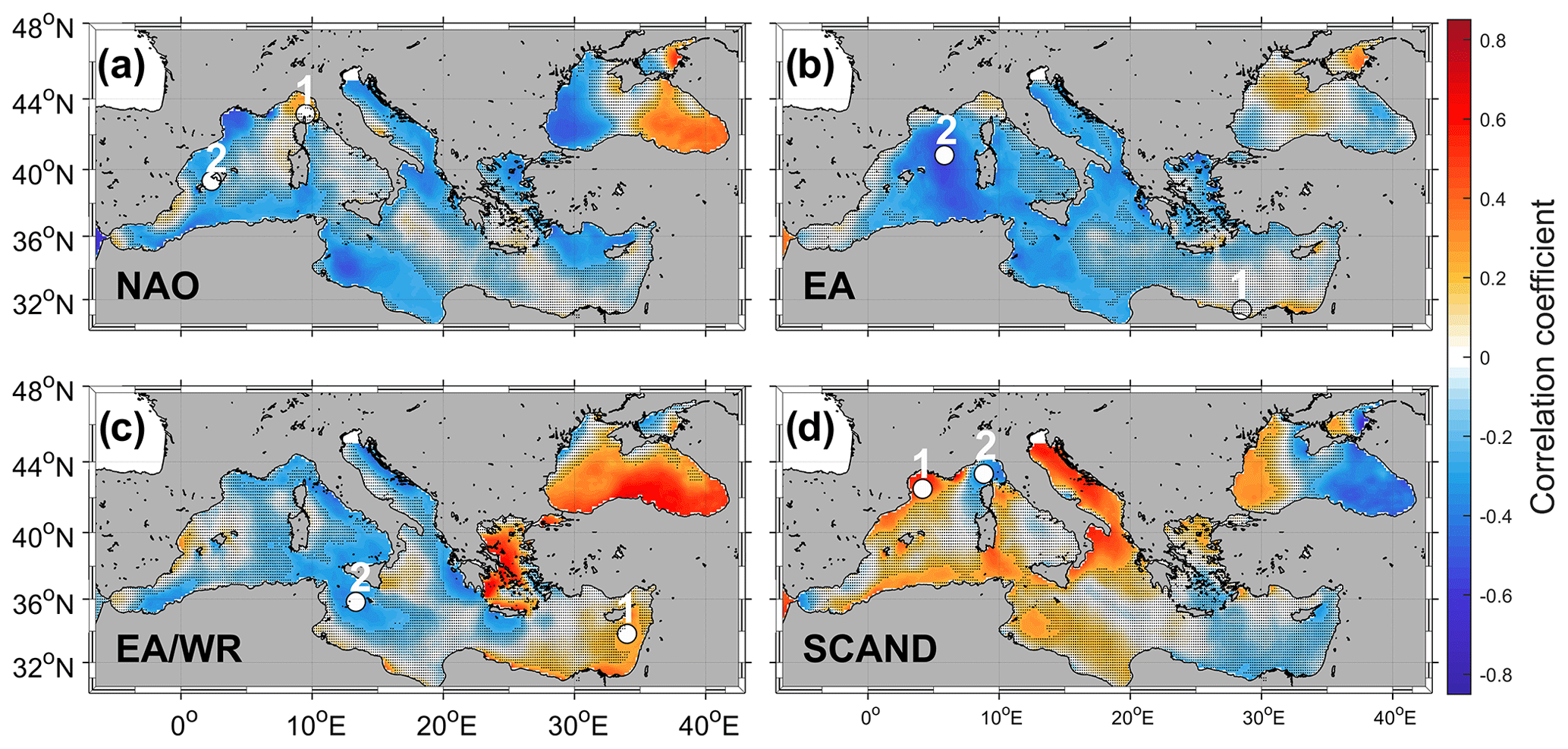
Figure 8Pearson correlation coefficient of winter mean 99th percentile SWH Mediterranean Sea series and (a) NAO, (b) EA, (c) EA/WR, and (d) SCAND winter mean indices. Dotting indicates no significant values at the 90 % confidence interval. The white points show (1) the maximum positive and (2) the maximum negative value of the correlation coefficient.
3.2 Synoptic atmospheric composites associated with extreme wave patterns
The analysis of the atmospheric signature associated with extreme SWH is performed by computing the composites of extreme SWH, atmospheric mean sea level pressure (MSLP), and 10 m wind velocity (U10). The objective is to find the atmospheric pattern that is associated with extreme winter waves. The procedure to build the composites is as follows.
-
First, we select the locations with the highest correlations between SWH99 and each of the atmospheric indices (points labeled no. 1 for maximum positive correlation and no. 2 for maximum negative correlation in Fig. 7 and Fig. 8 for the North Atlantic and Mediterranean Sea, respectively).
-
We select the time steps for which the original 3-hourly SWH time series at points no. 1 and no. 2 exceed SWH99 (two values each month are selected because the monthly number of data points is 224–248 depending on the month of the year).
-
Finally, we compute the composites for SWH, U10, and MSLP over the whole domain for all selected dates.
Note that the locations labeled no. 1 and no. 2 in each map represent the largest positive and negative correlations with the corresponding index. The composite maps are thus interpreted as the synoptic patterns associated with positive and negative phases (respectively) of the climate index leading to extreme waves.
3.2.1 Atlantic Ocean
The composite for U10 and MSLP built using location no. 1 (positive correlation between SWH99 and NAO) (Fig. 9a) shows the typical configuration associated with the positive NAO phase that is characterized by low pressures across high latitudes in the North Atlantic and high pressures over the central North Atlantic, the eastern United States, and western Europe. This composite is characterized by a strong westerly wind stream crossing the central North Atlantic whose fetch generates large waves at the western part of the British Islands and south of Iceland (SWH > 9 m). A similar relationship was demonstrated dynamically by Wolf and Woolf (2006). By contrast, in the south of the North Atlantic Ocean in the Azores region, a positive NAO phase results in low SWH99 values (SWH≈4 m). This pattern corresponds to the first EOF (Fig. 5a and Fig. 5, point 1, for the spatial mode and its amplitude, respectively) when, for positive values of the PC, positive anomalies are presented in the north part of the basin and negative anomalies in the central part (the opposite for negative values of the PC). The composite for the positive phase of EA shows a similar structure as the one obtained for the positive phase of NAO, but with the North Atlantic cyclone shifted southwards and with the high pressures covering the entire Atlantic at 30∘ N (Fig. 9b). Maximum waves associated with the EA are obtained in the central Atlantic as a result of the southward winds blowing from Greenland. This pattern corresponds to the second EOF (Fig. 5c and Fig. 5, point 2). The composite for the EA/WR positive phase shows a low-pressure system at 40∘ W, with the maximum extreme waves located to the east of Newfoundland (Fig. 9c). Finally, the atmospheric composite for the positive SCAND phase shows a cyclone (at 40∘ N) generating extreme waves smaller than obtained with the previous three composites, with values of SWH below 7 m (Fig. 9d). This pattern is associated with the first EOF when its amplitude takes negative values (see Fig. 5b and Fig. 5, point 1), also corresponding to the atmospheric situation related to the negative phase of NAO (see Fig. 10a). For the negative EA phase, the cyclone is located between Greenland and Iceland, generating a strong wind jet from the coast of Canada to Ireland (Fig. 10b). At this point, we want to remark that since we are analyzing the negative correlations, the values displayed in Table 2 have to be changed in sign. The second EOF (Fig. 5c) according to Table 2 is related to the composite built for the maximum negative correlation between SWH99 and the EA index (Fig. 10b). Composites for the negative phase of EA/WR are characterized by a western shift of the Icelandic Low that generates strong zonal winds between 50 and 60∘ N with maximum extreme waves located between the south of Ireland and north of Spain (Fig. 10c). The Icelandic Low for the negative SCAND phase is shifted northeast of Iceland with winds blowing southwestwards and extreme waves located between Iceland and Great Britain (Fig. 10d). This composite is associated with the first EOF (Fig. 5b), thus having a correlation with the positive NAO phase (see also Fig. 9a for comparison).
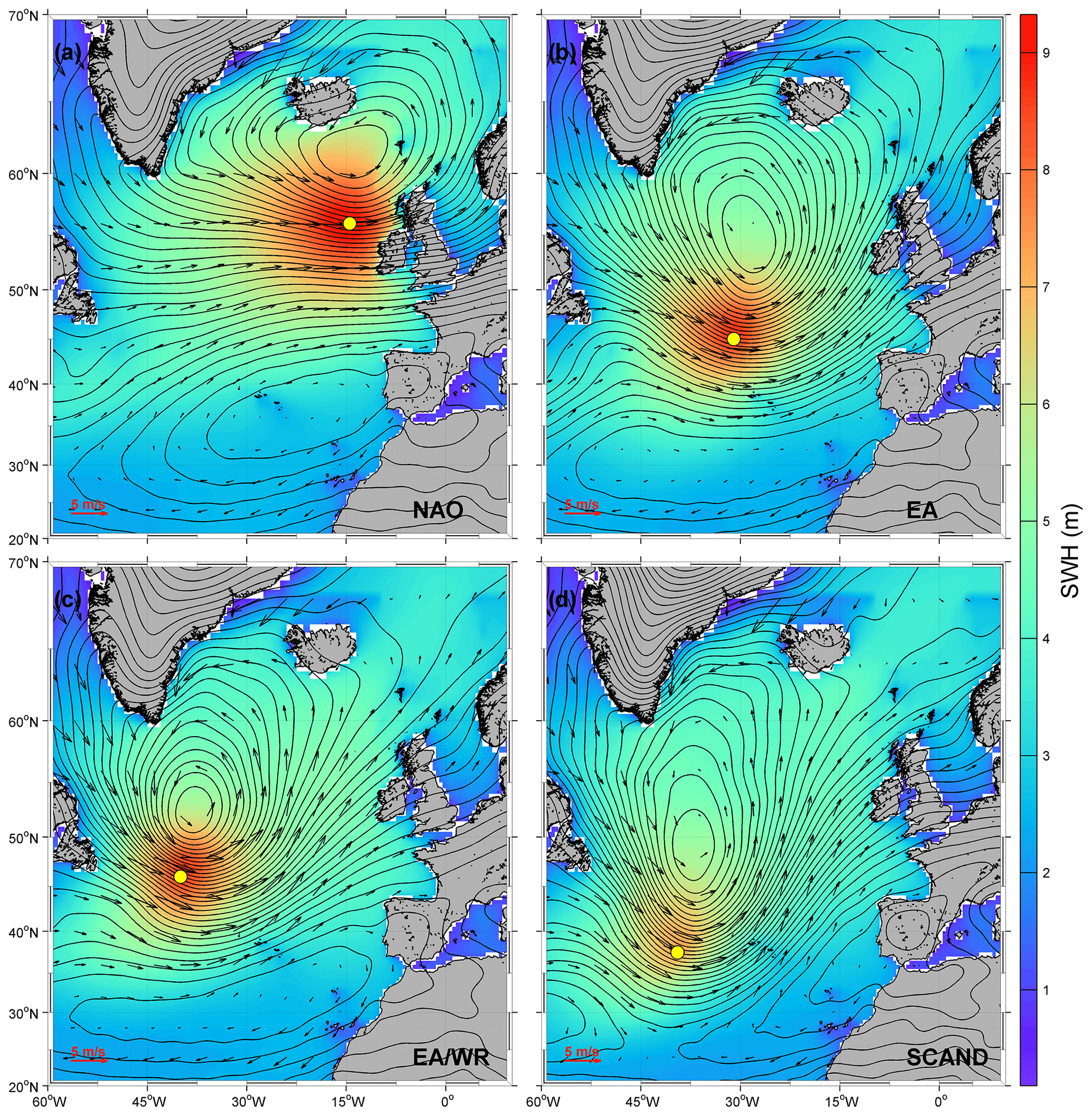
Figure 9Winter atmospheric situations for the positive phase of (a) NAO, (b) EA, (c) EA/WR, and (d) SCAND indices in the North Atlantic Ocean. The vectors represent the 10 m wind speed in meters per second; the contours represent the sea level pressure (Pa), and the color range is the mean value of SWH in meters. The red left bottom arrow represents the wind scale.
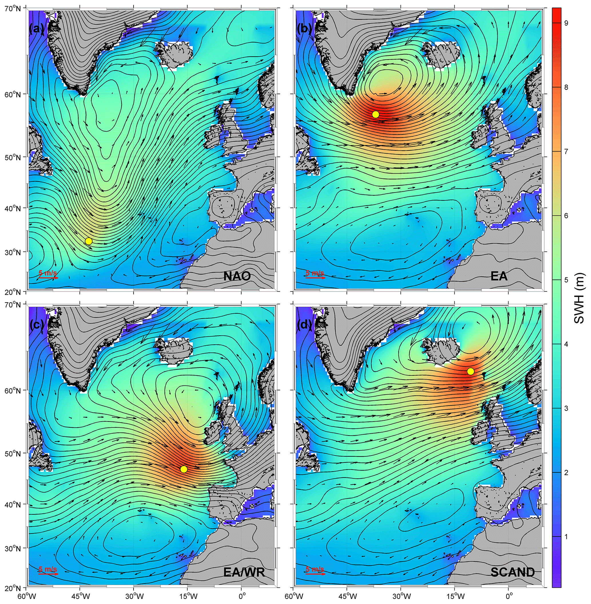
Figure 10Winter atmospheric situations for the negative phase of (a) NAO, (b) EA, (c) EA/WR, and (d) SCAND indices in the North Atlantic Ocean. The vectors represent the 10 m wind speed in meters per second; the contours represent the sea level pressure (Pa), and the color range is the mean value of SWH in meters. The red left bottom arrow represents the wind scale.
3.2.2 Mediterranean Sea
In the Mediterranean Sea, for the positive correlations between indices and extreme waves, we choose locations near the coast since negative correlations dominate the entire basin (Fig. 8). The atmospheric composite for the positive NAO phase displays a low-pressure system in the north of Italy with associated eastward winds in the western and central basins (Fig. 11a). These conditions are strongly associated with the atmospheric situations discussed in Trigo et al. (1999) for the cyclogenetic activity during winters. This composite is related to the distribution of extreme waves shown by the third EOF (Fig. 6d). Note that the amplitude of this mode is positively correlated with NAO according to Table 2. The composite for the positive EA phase shows intense cyclogenetic activity in the eastern Mediterranean Sea with its center of action over Cyprus, which generates strong winds and waves north of Egypt (Fig. 11b). This index, as shown in Table 2, is negatively correlated with the amplitude of the second EOF whose pattern presents large values for the extreme wave anomalies over the eastern Mediterranean Sea (Fig. 6c); in other words, a positive EA results in larger SWH99 in the eastern basin, as displayed in Fig. 11b. Regarding the positive EA/WR phase, the resulting composite presents a very similar pattern for surface pressure, winds, and waves as the one obtained for the positive EA phase (see Fig. 11b and c). The EA/WR index is also negatively correlated with the amplitude of the second EOF (Table 2), resulting in the same distribution of extreme waves as previously explained regarding the EA. Finally, the composite for the positive SCAND index displays a cyclonic structure in the northwestern part of the Mediterranean Sea – between Corsica and Sardinia – with winds blowing southwards at the Gulf of Lion (Fig. 11d). The SCAND index is positively correlated with the amplitude of the second EOF (Table 2), indicating larger (smaller) SWH99 in the western (eastern) Mediterranean during its positive phase.
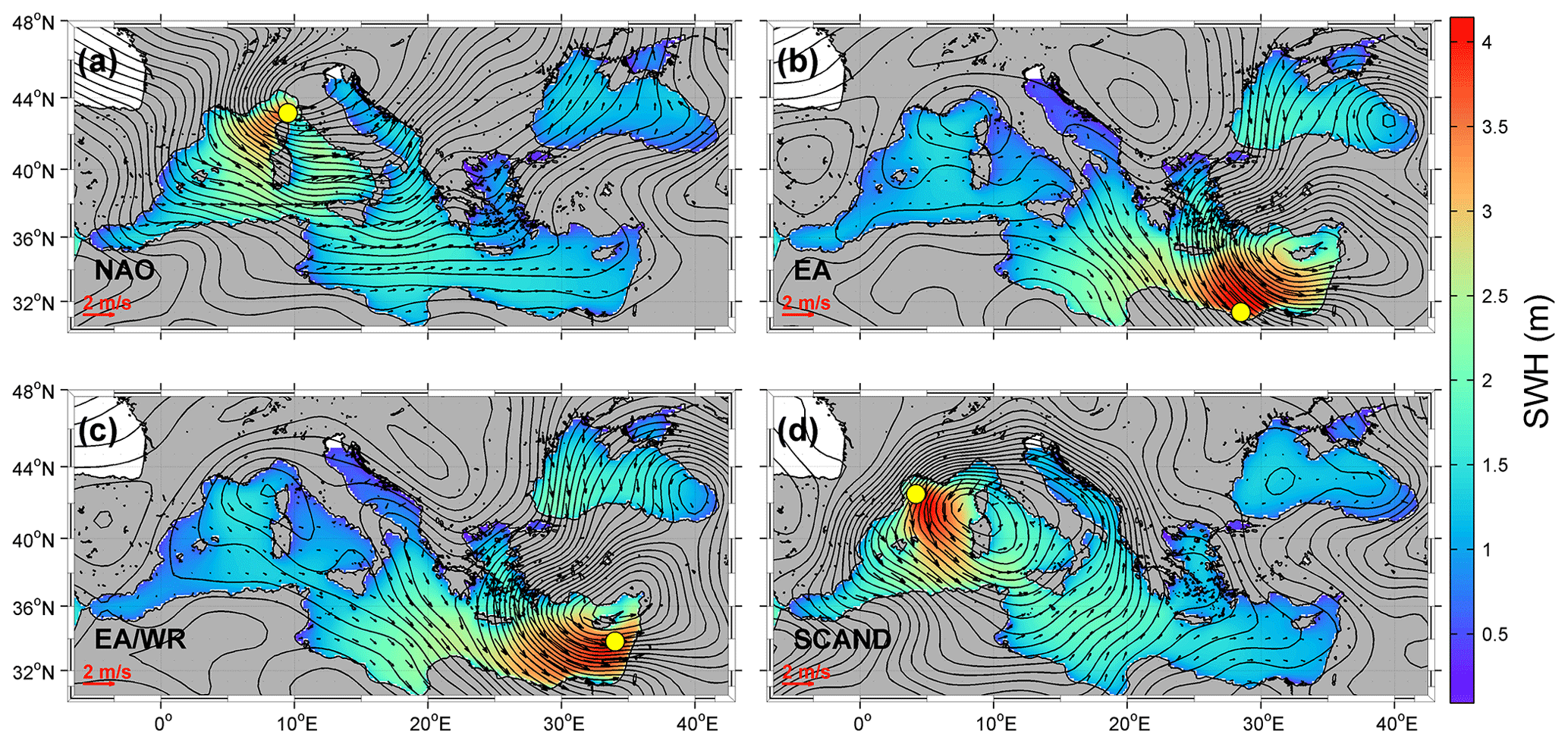
Figure 11Winter atmospheric situations for the positive phase of (a) NAO, (b) EA, (c) EA/WR, and (d) SCAND indices in the Mediterranean Sea. The vectors represent the 10 m wind speed in meters per second; the contours represent the sea level pressure (Pa), and the color range is the mean value of SWH in meters. The red left bottom arrow represents the wind scale.
For the negative phases during winters, the composite for the NAO displays a weak cyclone over the Ligurian Sea (Fig. 12a). In this situation, however, the pressure gradient is weaker, and due to the small fetch the resulting extreme waves are small (below 3.5 m in SWH). Regarding the negative phase of the EA index, the composite shows a strong cyclone centered over Italy with a large pressure gradient over the northwestern Mediterranean Sea. This situation generates strong winds between the Balearic Islands and Corsica and Sardinia, generating large waves in this area. The EA index is negatively correlated with the amplitude of the second EOF (see Fig. 6c). For the negative phase of EA/WR, the composite shows a low-pressure system over the Ionian Sea with a strong pressure gradient between Sicily and Tunisia, resulting in large extreme waves in this passage (Fig. 12c). This index is negatively correlated with the amplitude of the second EOF (Table 2), suggesting that for positive anomalies of SWH99 (see Fig. 6c) a negative phase of the EA/WR index results in an increase in extreme waves. Finally, the composite for the negative phase of the SCAND index displays a low-pressure system over the north of Italy. Although the pressure gradient associated with this low system is intense north of Corsica, the small fetch encourages the formation of extreme waves (Fig. 12d).
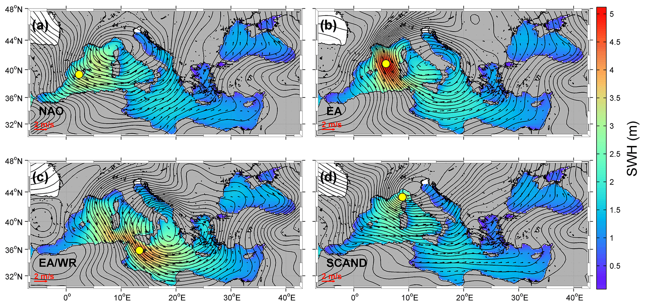
Figure 12Winter atmospheric situations for the negative phase of (a) NAO, (b) EA, (c) EA/WR, and (d) SCAND indices in the Mediterranean Sea. The vectors represent the 10 m wind speed in meters per second; the contours represent the sea level pressure (Pa), and the color range is the mean value of SWH in meters. The red left bottom arrow represents the wind scale.
This work presents a new methodology to study extreme wave climate and the atmospheric synoptic conditions responsible for extreme waves. Winds and pressure are obtained by computing the composites corresponding to the monthly values of the 99th percentile of the significant wave height. As a result, it is possible to infer changes in the location and intensity of extreme waves through an understanding of the variability of climatic patterns (widely studied). This approach could be of interest for all activities related to the prognosis of extreme waves, such as the design of offshore structures, among others.
The study is focused on the North Atlantic Ocean and the Mediterranean Sea, although the methodology can be extrapolated to any region in order to get a deeper insight into the seasonal and interannual variability of extreme wave climate. In the present work, interannual variability has been analyzed using empirical orthogonal functions, which have been correlated against the four main climate indices of variability in the area, i.e., NAO, EA, EA/WR, and SCAND. Finally, the most reliable atmospheric situation associated with each climatic pattern is discussed using the described methodology.
The extreme waves climate has a large seasonal signal in both the North Atlantic Ocean and the Mediterranean Sea. Our results also indicate a large intra-annual variability in the central part of the Mediterranean Sea and lower variability in the Alboran and Ligurian sub-basins, in agreement with Sartini et al. (2017) wherein they exhibited different degrees of seasonality depending on the main mesoscale meteorological features of the locations analyzed. Concerning the long-term trend of extreme waves, it is predominantly negative, although there are some areas, such as in the center of the North Atlantic Ocean and in the Aegean Sea, where the value of the tendency is positive. These results are not in line with the studies of Young et al. (2011) and Young and Ribal (2019) because here we assess only the extreme wave values during the winter season when most of the maximum SWHs occur.
Regarding climatic modes of variability, we found that the NAO and the SCAND indices are the leading modes of climatic variability affecting extreme waves in the North Atlantic Ocean during winters. The positive NAO phase increases extreme waves in the northern North Atlantic, while the negative NAO phase results in an increase in extreme waves in the southern North Atlantic, in accordance with Hurrell et al. (2003). By contrast, a positive SCAND index increases extreme waves in the southern North Atlantic, while a negative SCAND index increases extreme waves in the north part of the North Atlantic Ocean, as Martínez-Asensio et al. (2016) also pointed out. To a lesser extent, the EA also influences extreme waves in the North Atlantic Ocean, as Izaguirre et al. (2010) also concluded. While the positive EA phase drives extreme wave climate in the central North Atlantic, the negative phase controls extreme wave climate at higher and lower latitudes (see Fig. 7b). For future studies, a wavelet coherence analysis (Torrence and Compo, 1998) between the main climatic indices and extreme waves will provide additional information on the dominant modes of variability and how they vary in time.
The interannual variability of extreme waves during winters in the Mediterranean Sea is dominated, to a large extent, by the negative phase of EA, with a larger effect in the western basin. A positive NAO phase also has an influence on extreme waves, although they are smaller in the whole Mediterranean Sea.
Caires et al. (2006) reported that the wave climate is expected to change by a small amount in response to climate change (below 5 % between 1990 and 2080). The results presented here could be used to project climate and to develop appropriate studies for coastal protection, improving numerical models and defining long-term wave energy conversion strategies; the climatic patterns of the NAO will dominate the extreme wave climate in the North Atlantic Ocean to a larger extent in future scenarios according to Gleeson et al. (2017).
All data are accessible at https://polar.ncep.noaa.gov/waves/hindcasts/nopp-phase2.php (WAVEWATCH III, 2018) and https://www.cpc.ncep.noaa.gov/data/teledoc/telecontents.shtml (NWS2020).
AO conceived the idea of the study with the support of VMM, GS, and MM. AO and VMM developed the methodology with the support of MM and GS. VMM produced the results with the support of AO and MM. MM and GS analyzed the results with the support of AO and VMM. All authors contributed to writing the paper.
Alejandro Orfila is a member of the editorial board of Ocean Dynamics and Frontiers in Marine Sciences. Marta Marcos is a member of the editorial board of Frontiers in Marine Sciences.
The authors acknowledge financial support from MINECO/FEDER through project MORFINTRA/MUSA (grant no. CTM2015-66225-C2-2-P) and from the Ministerio de Ciencia, Innovación y Universidades through the MOCCA project (grant no. RTI2018-095441-B-C21). In addition, the authors thank NCEP and NOAA CPC for the freely available data that have been used in this article. Verónica Morales-Márquez is supported by an FPI grant from the Ministerio de Ciencia, Innovación y Universidades. In addition, Verónica Morales-Márquez acknowledges the 2019 EGU OSPP award for this work. This work was partially performed while Alejandro Orfila was a visiting scientist in the Earth, Environmental and Planetary Sciences Department at Brown University through a Ministerio de Ciencia, Innovación y Universidades fellowship (grant no. PRX18/00218). We are deeply grateful for comments from David Woolf and one anonymous referee.
This research has been supported by the Ministerio de Ciencia e Innovación (grant nos. FPI2016, CTM2015-66225-C2-2-P, RTI2018-095441-B-C21, and PRX18/00218) and the European Geosciences Union (EGU OSPP 2019 grant).
This paper was edited by Judith Wolf and reviewed by David Woolf and one anonymous referee.
Amante, C. and Eakins, B. W.: ETOPO1 Arc-Minute Global Relief Model: procedures, data sources and analysis, free access report from National Geophysical Data Center, Marine Geology and Geophysics Division Boulder, Colorado, NOAA Technical Memorandum (NESDIS NGDC-24), 2009. a
Ardhuin, F., Rogers, E., Babanin, A. V., Filipot, J.-F., Magne, R., Roland, A., van der Westhuysen, A., Queffeulou, P., Lefevre, J.-M., Aouf, L., and Collard, F.: Semiempirical dissipation source functions for ocean waves. Part I: Definition, calibration, and validation, J. Phys. Oceanogr., 40, 1917–1941, 2010. a
Barnston, A. G. and Livezey, R. E.: Classification, seasonality and persistence of low-frequency atmospheric circulation patterns, Month. Weather Rev., 115, 1083–1126, 1987. a, b
Caires, S., Swail, V. R., and Wang, X. L.: Projection and analysis of extreme wave climate, J. Climate, 19, 5581–5605, 2006. a, b
Castelle, B., Dodet, G., Masselink, G., and Scott, T.: Increased winter-mean wave height, variability, and periodicity in the Northeast Atlantic over 1949–2017, Geophy. Res. Lett., 45, 3586–3596, 2018. a
Chawla, A., Spindler, D., and Tolman, H. L.: A thirty year wave hindcast using the latest NCEP Climate Forecast System Reanalysis winds, in: Proc. 12th Int. Workshop on Wave Hindcasting and Forecasting, MMAB Contribution, Kohala Coast, Hawaii, HI, 296, 2011. a
Chawla, A., Spindler, D., and Tolman, H.: 30 Year Wave Hindcasts using WAVEWATCH III with CFSR winds-Phase I. MMAB Contribution No. 302: NCEP/NOAA, 12p., College Park, MD, United States of America, https://doi.org/10.1016/j.ocemod.2012.07.005, 2012. a, b
Chawla, A., Spindler, D. M., and Tolman, H. L.: Validation of a thirty year wave hindcast using the Climate Forecast System Reanalysis winds, Ocean Model., 70, 189–206, 2013. a
Environmental Modeling Center, NOAA NWS National Centers for Environmental Prediction: WAVEWATCH III 30-year Hindcast Phase 2, https://polar.ncep.noaa.gov/waves/hindcasts/nopp-phase2.php, last acces: 25 February 2018. a
Gallagher, S., Tiron, R., and Dias, F.: A long-term nearshore wave hindcast for Ireland: Atlantic and Irish Sea coasts (1979–2012), Ocean Dynam., 64, 1163–1180, 2014. a
Gallagher, S., Gleeson, E., Tiron, R., McGrath, R., and Dias, F.: Twenty-first century wave climate projections for Ireland and surface winds in the North Atlantic Ocean, Adv. Sci. Res., 13, 75–80, 2016. a
Gleeson, E., Gallagher, S., Clancy, C., and Dias, F.: NAO and extreme ocean states in the Northeast Atlantic Ocean, Adv. Sci. Res., 14, 23–33, 2017. a
Gleeson, E., Clancy, C., Zubiate, L., Janjić, J., Gallagher, S., and Dias, F.: Teleconnections and Extreme Ocean States in the Northeast Atlantic Ocean, Adv. Sci. Res., 16, 11–29, 2019. a
Hurrell, J. W., Kushnir, Y., Ottersen, G., and Visbeck, M.: An overview of the North Atlantic oscillation, The North Atlantic Oscillation: climatic significance and environmental impact, Geoph. Monog.-Am. Geophys. Union, 1–35, 2003. a, b
Izaguirre, C., Mendez, F. J., Menendez, M., Luceño, A., and Losada, I. J.: Extreme wave climate variability in southern Europe using satellite data, J. Geophys. Res.-Oceans, 115, C04009, https://doi.org/10.1029/2009JC005802, 2010. a, b, c, d, e
Izaguirre, C., Menéndez, M., Camus, P., Méndez, F. J., Mínguez, R., and Losada, I. J.: Exploring the interannual variability of extreme wave climate in the Northeast Atlantic Ocean, Ocean Model., 59, 31–40, 2012. a, b
Janssen, P. A.: Progress in ocean wave forecasting, J. Comput. Phys., 227, 3572–3594, 2008. a
Lin, Y., Oey, L.-Y., and Orfila, A.: Two `faces' of ENSO-induced surface waves during the tropical cyclone season, Prog. Oceanogr., 175, 40–54, https://doi.org/10.1016/j.pocean.2019.03.004, 2019. a
Lionello, P. and Sanna, A.: Mediterranean wave climate variability and its links with NAO and Indian Monsoon, Climate Dynam., 25, 611–623, 2005. a
Marshall, J., Kushnir, Y., Battisti, D., Chang, P., Czaja, A., Dickson, R., Hurrell, J., McCartney, M., Saravanan, R., and Visbeck, M.: North Atlantic climate variability: phenomena, impacts and mechanisms, Int. J. Climatol., 21, 1863–1898, 2001. a
Martínez-Asensio, A., Tsimplis, M. N., Marcos, M., Feng, X., Gomis, D., Jordà, G., and Josey, S. A.: Response of the North Atlantic wave climate to atmospheric modes of variability, Int. J. Climatol., 36, 1210–1225, 2016. a, b
Méndez, F. J., Menéndez, M., Luceño, A., and Losada, I. J.: Estimation of the long-term variability of extreme significant wave height using a time-dependent peak over threshold (pot) model, J. Geophys. Res.-Oceans, 111, C07024, https://doi.org/10.1029/2005JC003344, 2006. a
Menéndez, M., Méndez, F. J., Losada, I. J., and Graham, N. E.: Variability of extreme wave heights in the northeast Pacific Ocean based on buoy measurements, Geophys. Res. Lett., 35, L22607, https://doi.org/10.1029/2008GL035394, 2008. a
Menéndez, M., Méndez, F. J., Izaguirre, C., Luceño, A., and Losada, I. J.: The influence of seasonality on estimating return values of significant wave height, Coast. Eng., 56, 211–219, 2009. a, b
Morales-Márquez, V., Orfila, A., Simarro, G., Gómez-Pujol, L., Álvarez-Ellacuría, A., Conti, D., Galán, Á., Osorio, A. F., and Marcos, M.: Numerical and remote techniques for operational beach management under storm group forcing, Nat. Hazards Earth Syst. Sci., 18, 3211–3223, https://doi.org/10.5194/nhess-18-3211-2018, 2018. a
National Weather Service, Climate Prediction Center: Northern Hemisphere teleconnection patterns, https://www.cpc.ncep.noaa.gov/data/teledoc/telecontents.shtml, last acces: 27 February 2020.
Orejarena-Rondón, A. F., Sayol, J. M., Marcos, M., Otero, L., Restrepo, J. C., Hernández-Carrasco, I., and Orfila, A.: Coastal impacts driven by sea-level rise in Cartagena de Indias, Front. Mar. Sci., 6, 614, https://doi.org/10.3389/fmars.2019.00614, 2019. a
Polton, J. A., Lewis, D. M., and Belcher, S. E.: The role of wave-induced Coriolis-Stokes forcing on the wind-driven mixed layer, J. Phys. Oceanogr., 35, 444–457, 2005. a
Ponce de León, S., Orfila, A., and Simarro, G.: Wave energy in the Balearic Sea, Evolution from a 29 year spectral wave hindcast, Renew. Energ., 85, 1192–1200, 2016. a
Saha, S.: Documentation of the Hourly Time Series from the NCEP Climate Forecast System Reanalysis (1979–2009), free access report from EMC/NCEP/NOAA, 2009. a
Sartini, L., Besio, G., and Cassola, F.: Spatio-temporal modelling of extreme wave heights in the Mediterranean Sea, Ocean Model., 117, 52–69, 2017. a, b
Tolman, H. L.: User manual and system documentation of WAVEWATCH III TM version 3.14, MMAB Contribution, College Park, MD, U.S.A., p.220, 2009. a
Torrence, C. and Compo, G. P.: A practical guide to wavelet analysis, B. Am. Meteorol. Soc., 79, 61–78, 1998. a
Trigo, I. F., Davies, T. D., and Bigg, G. R.: Objective climatology of cyclones in the Mediterranean region, J. Climate, 12, 1685–1696, 1999. a
Trigo, I. F., Bigg, G. R., and Davies, T. D.: Climatology of cyclogenesis mechanisms in the Mediterranean, Mon. Weather Rev., 130, 549–569, 2002. a
Vinoth, J. and Young, I.: Global estimates of extreme wind speed and wave height, J. Climate, 24, 1647–1665, 2011. a
Wallace, J. M. and Gutzler, D. S.: Teleconnections in the Geopotential Height Field during the Northern Hemisphere Winter, Mon. Weather Rev., 109, 784–812, https://doi.org/10.1175/1520-0493(1981)109<0784:TITGHF>2.0.CO;2, 1981. a
Wang, X. L. and Swail, V. R.: Changes of extreme wave heights in Northern Hemisphere oceans and related atmospheric circulation regimes, J. Climate, 14, 2204–2221, 2001. a
Wang, X. L. and Swail, V. R.: Trends of Atlantic wave extremes as simulated in a 40-year wave hindcast using kinematically reanalyzed wind fields, J. Climate, 15, 1020–1035, 2002. a
Weiss, J., Bernardara, P., and Benoit, M.: Formation of homogeneous regions for regional frequency analysis of extreme significant wave heights, J. Geophys. Res.-Oceans, 119, 2906–2922, 2014. a
Wolf, J. and Woolf, D. K.: Waves and climate change in the north-east Atlantic, Geophys. Res. Lett., 33, L06604, https://doi.org/10.1029/2005GL025113, 2006. a
Woolf, D. K., Challenor, P., and Cotton, P.: Variability and predictability of the North Atlantic wave climate, J. Geophys. Res.-Oceans, 107, 3145, https://doi.org/10.1029/2001JC001124, 2002. a
Young, I., Zieger, S., and Babanin, A. V.: Global trends in wind speed and wave height, Science, 332, 451–455, 2011. a, b
Young, I., Vinoth, J., Zieger, S., and Babanin, A. V.: Investigation of trends in extreme value wave height and wind speed, J. Geophys. Res.-Oceans, 117, C00J06, https://doi.org/10.1029/2011JC007753, 2012. a
Young, I. R. and Ribal, A.: Multiplatform evaluation of global trends in wind speed and wave height, Science, 364, 548–552, 2019. a