the Creative Commons Attribution 3.0 License.
the Creative Commons Attribution 3.0 License.
Observations of brine plumes below melting Arctic sea ice
In sea ice, interconnected pockets and channels of brine are surrounded by fresh ice. Over time, brine is lost by gravity drainage and flushing. The timing of salt release and its interaction with the underlying water can impact subsequent sea ice melt. Turbulence measurements 1 m below melting sea ice north of Svalbard reveal anticorrelated heat and salt fluxes. From the observations, 131 salty plumes descending from the warm sea ice are identified, confirming previous observations from a Svalbard fjord. The plumes are likely triggered by oceanic heat through bottom melt. Calculated over a composite plume, oceanic heat and salt fluxes during the plumes account for 6 and 9 % of the total fluxes, respectively, while only lasting in total 0.5 % of the time. The observed salt flux accumulates to 7.6 kg m−2, indicating nearly full desalination of the ice. Bulk salinity reduction between two nearby ice cores agrees with accumulated salt fluxes to within a factor of 2. The increasing fraction of younger, more saline ice in the Arctic suggests an increase in desalination processes with the transition to the “new Arctic”.
- Article
(6015 KB) - Full-text XML
- BibTeX
- EndNote


In the Arctic Ocean, sea ice is an effective barrier for exchange between the ocean and atmosphere. The presence of sea ice, however, depends on a delicate balance between the atmospheric and oceanic heat fluxes. The inflowing Atlantic water contains enough heat to melt the Arctic sea ice in a few years (Turner, 2010), and a small change in oceanic heat flux can have huge implications for the heat balance at the interface. Understanding the processes that control vertical heat fluxes under the sea ice is important to understand the response of sea ice to a changing climate (Carmack et al., 2015). The interplay between heat and salt exchange at the ice–ocean interface can work to enhance or reduce sea ice melt in the Arctic Ocean (Sirevaag, 2009).
While sea ice in bulk is a source of fresh water to the upper ocean, the sea ice consists of fresh ice surrounding pockets of liquid brine connected through a network of channels and capillaries (Petrich and Eicken, 2010). The brine remains at its salinity-determined freezing point in thermal equilibrium with the surrounding ice, and brine salinity and volume adjust to temperature changes by growing or melting fresh ice.
Over time, salt is lost from the sea ice. The timing of the salt release and how the salt is distributed in the water column is important in the evolution of the Arctic mixed layer. The main desalination processes of sea ice are gravity drainage and flushing of surface meltwater and melt ponds (Notz and Worster, 2009). While melt ponds are present only in advanced stages of melt, gravity drainage occurs throughout the seasons. Ice permeability is a controlling factor for gravity drainage, increasing with temperature as the ice warms (Golden et al., 1998). When sea ice warms to within a certain critical temperature range, full-depth brine convection and desalination can occur, even before the onset of melt (Jardon et al., 2013). Furthermore, gravity drainage has been successfully modeled using a 1-D sea ice model and can be triggered both by atmospheric heat and bottom melt from oceanic heat (Griewank and Notz, 2013).
Despite the theoretical understanding and successful modeling of spring-time brine convection, observations are sparse. Brine drainage in response to atmospheric warming may have been the cause of observed salinity anomalies below sea ice in Storfjorden (Jardon et al., 2013). Still, the main evidence so far has been observations of saline plumes descending from warming landfast sea ice in a Svalbard fjord (Widell et al., 2006). It has been hypothesized that this form of desalination can occur on drifting Arctic sea ice, but so far this has remained unverified. The existence of such plumes can be important to the desalination of sea ice and the subsequent distribution of salinity in the upper water column, and they could thus affect the otherwise strong surface stratification typical below melting ice.
The first observations of brine plumes released from drifting sea ice in the Arctic Ocean are presented here. The observations were collected in June 2015 in the marginal ice zone (MIZ) north of Svalbard (Fig. 1). The data are a subset of a previously reported under-ice turbulence data set (Peterson et al., 2016, 2017) and part of the Norwegian Young Sea Ice Cruise (Granskog et al., 2016).
2.1 Turbulence instrument cluster
Under-ice turbulence measurements were made using a turbulence instrument cluster (TIC) deployed 1 m below the ice undersurface, relying on eddy covariance to calculate turbulent fluxes of momentum and scalars from point measurements of temperature, salinity, and currents. The cluster is fixed on a mast deployed through a hole in the sea ice and suspended on a wire, which allows for the adjustment of the instrument depth. The concept is well proven, and processing follows previous studies (McPhee, 2002; McPhee et al., 2008). A detailed description of the setup is given in Peterson et al. (2017) and briefly summarized below. Horizontal and vertical currents are rotated into the mean current direction (u) such that the cross-stream (v) and vertical (w) current averages zero for a given 15 min segment. The data gaps visible in Fig. 2 are due to two corrupt data files.
Heat flux is calculated from the covariance of temperature and vertical velocity,
where ρw is the water density and cp is the specific heat capacity of the water; angled brackets indicate a temporal mean, and primes indicate detrended values (fluctuations about a 15 min mean value). The heat flux is positive when warmer water is brought upward, and cold downward. Similarly, salinity flux is calculated as
where FS is positive when more saline water is brought upward, and fresher water moves down. Accumulated salt flux (units kg m−2) is calculated by adding up 15 min salt fluxes (m s−1) multiplied by the segment's duration (s) using salinity in kg m−3.

Figure 1Overview of the study region north of Svalbard, showing the drift track of the ice camp studied here, with its starting point marked by a cross. The positions of the Van Mijenfjorden study (Widell et al., 2006) and Whaler's Bay (Sirevaag, 2009) are shown for reference.
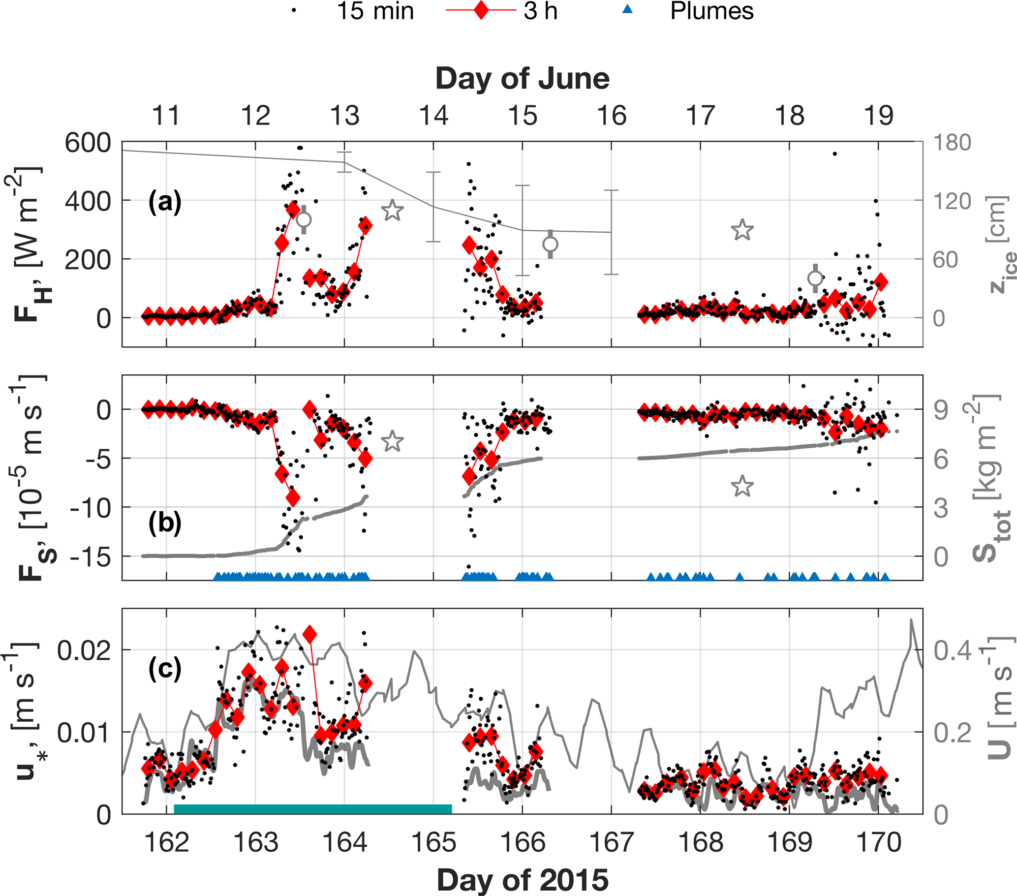
Figure 2Turbulent fluxes of (a) heat and (b) salt and (c) friction velocity are shown as 15 min data points (dots) and 3 h bin averages (diamonds). In (a), sea ice thickness is shown from manual measurements in the TIC hole (circles), hot wires (line), and two ice cores (stars). (b) Total salt content of the ice cores (stars) and measured cumulative salt flux, Stot, is given in kg m−2 (gray). Identified plumes are indicated by blue triangles. In (c), the sea ice drift speed (thin) and along-stream current (TIC, thick) are shown (gray), and the timing of a passing storm is indicated by the green line (Cohen et al., 2017).
The covariance of horizontal to vertical velocity gives the components of Reynold's stress, presented here as friction velocity,
where τ is the kinematic Reynolds stress magnitude.
The TIC data and the derived fluxes have been subjected to an extensive quality control, which is described in full in Peterson et al. (2017). The systematic approach is taken to ensure the validity of Taylor's hypothesis, which is crucial to the turbulent flux calculations. Taylor's hypothesis assumes that an eddy is essentially unchanged as it passes the measurement volume, allowing temporal measurements to be translated into spatial measurements. Each 15 min segment is split in 1 min half-overlapping subsegments, for which mean and root mean square values are calculated. This is compared to artificial Gaussian data and used to identify variability in the flow that violates Taylor's hypothesis, such as trends, rapid change in current direction, and swell. Segments that do not meet the criteria indicate unsteady flow and are excluded from the analysis. For the data presented here, 85 out of 612 segments (14 %) were rejected in quality control. Additional details on processing and data considerations are discussed in Sect. 6.
2.2 Auxiliary data
The TIC data are supplemented by atmospheric data from a 10 m tall weather mast (Cohen et al., 2017; Hudson et al., 2015) and navigational data from the research vessel Lance, which was anchored to the same ice floe during the drifts approximately 300–400 m away.
Environmental data from the upper ocean are obtained from profiles of temperature and salinity made using a microstructure sonde (Meyer et al., 2017a). The profiles were typically collected in sets of three casts repeated three times daily. Casts were made through a hydrohole about 50 m from the TIC site. Data were validated against the shipborne CTD (conductivity, temperature, depth) and corrected for sensor drift. The data were analyzed using the Thermodynamic Equation of Seawater 2010 (McDougall and Barker, 2011), and conservative temperature (Θ) and absolute salinity (SA) are used throughout.
Ice cores were sampled throughout the campaign for different ice types and sampling variables (Granskog et al., 2017). Two colocated ice cores with both temperature and salinity measurements were collected on the same ice floe as the flux measurements and are used in this study. Brine volume is calculated as Φ = Sbu∕Sbr, where Sbu is the bulk salinity, and brine salinity is calculated using the linear relation Sbr = 0.05411, which is adequate for warm ice (Notz et al., 2005).
In addition to the total height of the two ice cores, sea ice thickness is measured manually in the TIC hydrohole and in a grid of hot wires (Fig. 2). The manual measurements were read from a ruler (Amelie Meyer, personal communication, January 2017). Due to large but unknown uncertainty, the measurements in Fig. 2a are arbitrarily assigned ±15 cm error bars. A set of four hot wires were set up in an area of deformed sea ice, initially nearly 2 m thick (Rösel et al., 2016). The error bars in Fig. 2a are the standard deviation of the wires. Because of the spatial variability and uncertainties of the different measurements, all ice thickness data should be interpreted with care.
Observations were made from a drifting ice floe in the MIZ between 10 and 19 June (Figs. 1 and 3). The drift took place over the Yermak Plateau, where a branch of the warm West Spitsbergen Current flows across the plateau (Meyer et al., 2017b). Over 9 days, the floe drifted 185 km, with an average drift speed of 23 cm s−1, while water depths shoaled from about 2000 m to less than 1000 m over the Yermak Plateau. The floe had an approximate diameter of 1200 m and likely consisted of only first-year ice (Granskog et al., 2017). The TIC mast was deployed approximately 250 m from the floe edge. The ice drift was mostly parallel to the ice edge (Fig. 3).
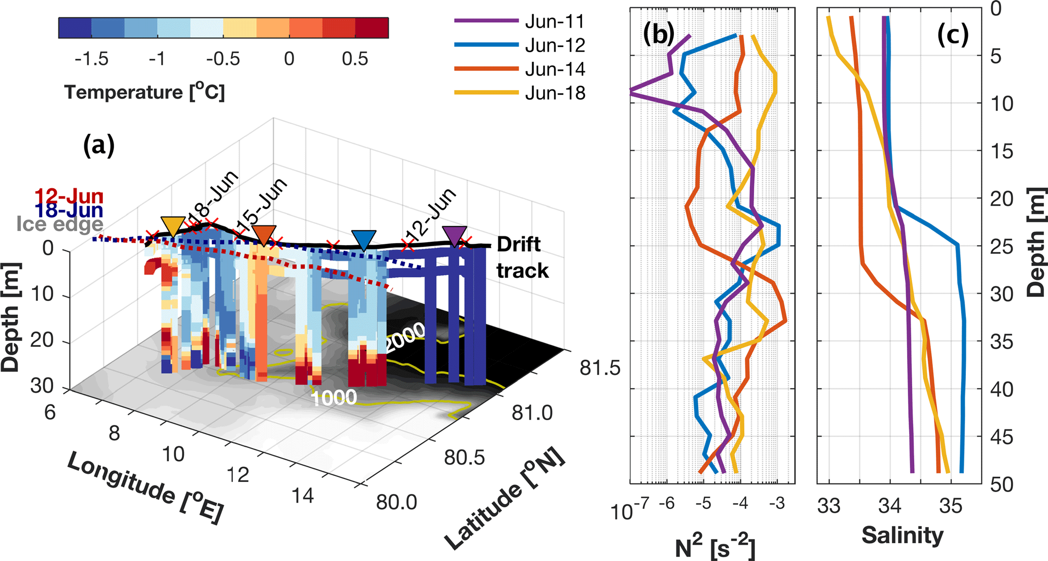
Figure 3Ocean and sea ice conditions over the course of the drift. (a) Drift track between 10 and 19 June (black) with daily ticks (crosses). Conservative temperature (colors) data are derived from a combination of vertical MSS profiles in the upper 30 m and TIC time series measurements from 1 and 5 m. The ice edge (50 % concentration) is shown for 12 and 18 June. Water depth is indicated in shading, with yellow isolines at 1000 and 2000 m. Triangles mark the location of (b) four profiles of stratification (N2) in the upper 50 m.
Temperature at 1 m below the ice averaged ΔT = 0.6 ∘C above freezing and was lowest on 11 June (ΔT = 0.1 ∘C) and highest (1.6 ∘C) during the storm on 13 June. Atlantic water flows along the topographic slope (Meyer et al., 2017b) and is often found at depths shallower than 30 m (defined as T > 0 ∘C, Fig. 3). Toward the end of the drift a warm intrusion is also observed at 5 to 10 m depth.
Stratification (Fig. 3b) in the upper 35 m varies significantly over the drift in and out of warmer waters. The mixed layer depth gradually changes from quite deep (> 30 m) in the beginning of the drift to non-existent at the end, varying with drift to and from areas where warm Atlantic water flows closer to the surface. First, there is a transition from waters of weak stratification (11 June) to gradually stronger surface stratification. On 12 June, the top of the pycnocline is about 20 m, reaching 27 m on 14 June. Towards the end of the drift, there is strong stratification continuously up to the surface, and there is no mixed layer present on 18 June.
Although sea ice thickness measurements are coarse, significant melt is evident over the drift (Fig. 2a). The measurements in the TIC hydrohole indicate a reduction from ∼ 100 to ∼ 40 cm between 12 and 18 June. Less melt was seen from the ice cores, with a reduction from 109 to 89 cm between 13 and 17 June. Hot wires measured a decrease from 174 to 87 cm over the measurements, although with a very large difference between sensors (variance of up to 46 cm). The ice around the hydrohole is likely melting faster compared to some distance away, and a representative sea ice reduction is likely somewhere between hydrohole and ice core values. Still, by the end of the measurements on 19 June, the ice was only a few decimeters thick, and the floe was disintegrating.

Figure 4Vertical profiles of sea ice (a) temperature, (b) bulk salinity, and (c) brine volume fraction. The ice cores are sampled about 100 m from the measurement site on 13 and 17 June. Average temperatures are −1.9 and −1.4 ∘C, and bulk salinities are 6.4 and 4.8 for 13 and 17 June, respectively. The typical 5 % threshold required for gravity drainage (Cox and Weeks, 1975) is indicated (c, dotted line).
From an ice coring site located approximately 100 m from the measurement site (Granskog et al., 2016) but on the same ice floe, two ice cores sampled on 13 and 17 June give some insight (Fig. 4). The ice core on 13 June shows 109 cm thick ice, with a 30 cm snow layer on top. The ice is rather warm, with a minimum temperature of −2.5 ∘C in the interior of the ice, increasing towards the surface (−1.3 ∘C) and the ice–ocean interface (−1.7 ∘C). The C-shaped temperature profile is indicative of a gradual warming from above. This is confirmed by atmospheric measurements reporting temperate conditions throughout the measurements on the floe, with temperatures ranging from −2 to +2 ∘C at 10 m of height between 7 and 20 June (Cohen et al., 2017). The snow layer was thick (∼ 30 cm), slowing heat exchange with the ice (Granskog et al., 2017). Comparison of the two ice cores reveals a decrease in bulk salinity from 6.4 to 4.8 in 4 days and a decrease in thickness of 20 cm, together causing a decrease in salt content of 2.8 kg m−2 (calculated by multiplying bulk salinity with ice thickness).
Eddy covariance measurements from 1 m below the ice undersurface reveal anticorrelated turbulent heat and salt fluxes (Fig. 2, r = −0.94) at a time of rapid bottom melt. Oceanic heat fluxes are directed towards the ice and reach several hundred W m−2 in response to a passing storm. Salt fluxes are directed down from the ice, exceeding −10−4 m s−1. The downward flux of salt is typical of freezing conditions, such as that observed in refreezing leads in the pack ice north of Alaska (McPhee and Stanton, 1996). During melting conditions, heat and salt fluxes are more typically both positive, as fresh meltwater is fluxed downward and is replaced by warmer water from below.
At the surface we generally find cooler, fresher water than below (Fig. 3), which is consistent with observed melting at the surface. The negative salt flux can thus not be caused by the entrainment of saline water from below. The observed heat and salt fluxes implies relatively cool, saline water above warmer, fresher water, which is an inherently unstable configuration that cannot be sustained over time. Unstable conditions can occur during a frontal passage, during which the observation point (ice floe) drifts from cool and saline water into an area of warmer, fresher water (McPhee et al., 1987; Sirevaag, 2009). When the floe drifts into recently ice-free waters, freshened from sea ice melt and warmed by the sun, cool water moving with the ice floe could be dragged over warm water, setting up an instability with appropriate gradients. The floe drifts over recently ice-free waters on two occasions, and for shorter periods such overturning might be expected, most notably in the last hours on 12 June concurrent with the decreasing flux magnitudes. However, the negative relationship between heat and salt fluxes is sustained over several days, during both increasing and decreasing temperatures, signaling a process that is continually feeding the instability. Negative correlation between the fluxes is consistent throughout the measurements. The turbulent heat flux is a likely forcing agent, as both fluxes increase with drift speed (Fig. 2c) and upper ocean temperature (Fig. 3a).
Brine released from warm sea ice is a possible explanation, as a source of cold, salty water sinking from the ice into the first meter of the ocean is consistent with negative salt flux and positive heat flux. Resemblance to the observations in the fjord study by Widell et al. (2006) inspired the search for an inferred mean plume structure. Events are identified in a similar manner, requiring at least five consecutive points at which w′ < 0, S′ > 1 × 10⁻⁵ and the salt flux magnitude, , exceeds 10−4 m s−1 or at least 5 times the root mean square value over the 15 min segment. A 60 s window centered on the peak value is used to construct a mean plume ensemble. For each iteration, the 15 min window is moved 5 min in order to also detect plumes otherwise falling on the edge of a window. Duplicate events are removed, leaving 131 identified plumes for the ensemble average, as shown in Fig. 5. Averaging is done using a bootstrap calculation (Emery and Thomson, 2001), which resamples the data 1000 times to obtain an estimate of the average value occurring by chance. The mean plume and its 95 % confidence interval from bootstrap calculations are shown in Fig. 5. The shading represents percentiles of the data as a display of the variability between plumes.
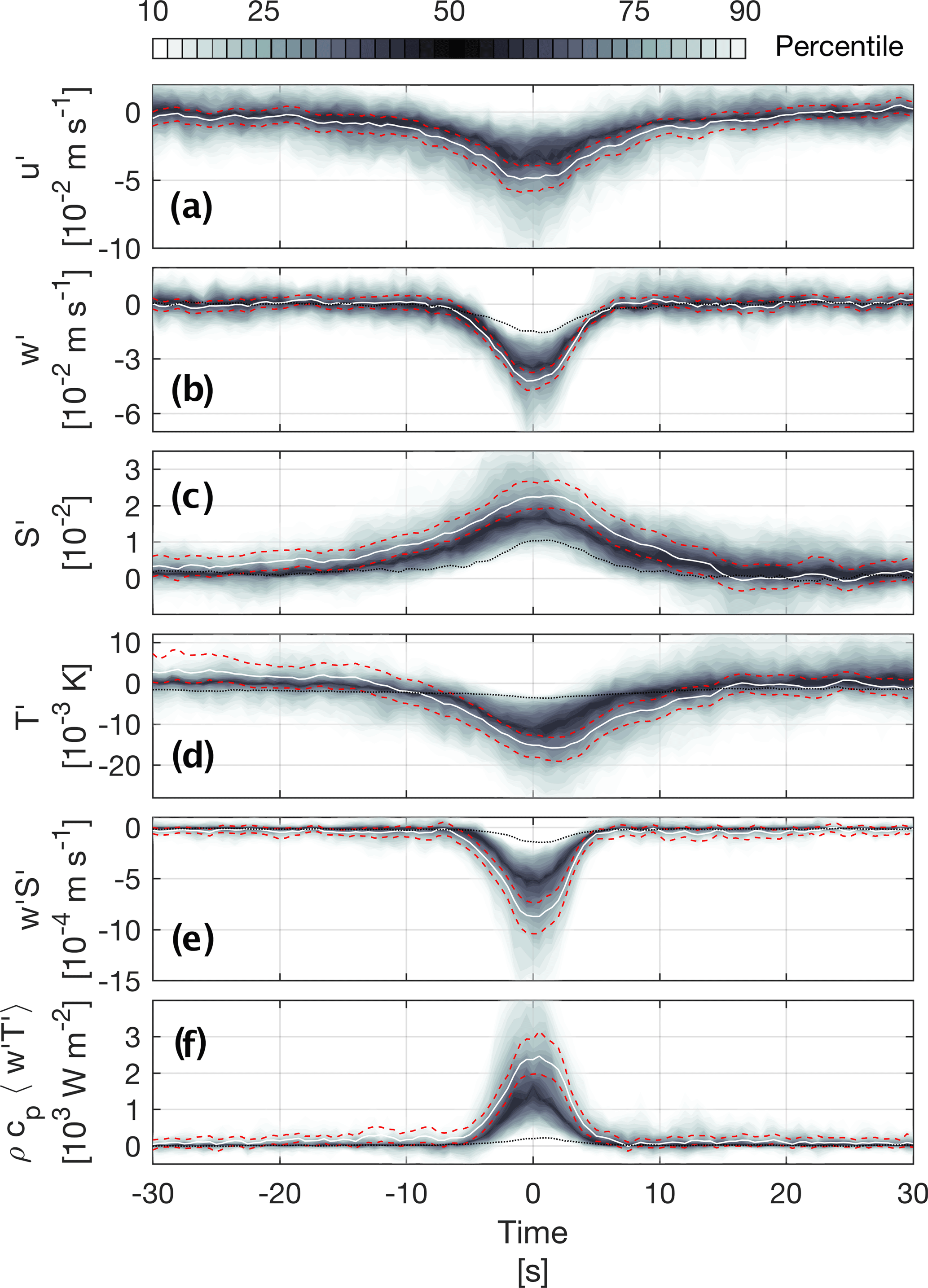
Figure 5Composite of 131 plumes identified using the peak in and presented in a 60 s window. Spread in the data is shown as percentiles (shading) overlain by the mean (white) and its 95 % confidence interval from bootstrap calculations (dashed red). Variables are fluctuations of (a) horizontal and (b) vertical velocity, (c) salinity, (d) temperature, and turbulent fluxes of (e) salt and (f) heat. The results from Widell et al. (2006) are shown for reference (black dotted lines).
The inferred plume is approximately symmetric in time about its peak. Anomalies in temperature and salinity gradually increase toward their peak values over about 10–15 s before they decrease again at the same pace. Vertical velocity perturbations, and thus also the fluxes, increase more abruptly, reaching a peak of 2–6 cm s−1 in about 7 s before returning to near zero. Horizontal velocity typically retards by around 5 cm s−1 during the plumes. Temperature and salinity anomalies deviate somewhat from symmetry, averaging positive (2.1 × 10⁻³ ∘C and 4.0 × 10⁻³) before the plume and approaching zero after. There is, however, considerable variation between individual events, and these are just characteristics of the mean structure. Individual plumes typically have sharper interfaces, and the smooth transitions in Fig. 5 are partly due to averaging. Salt and heat fluxes averaged over the 14 s surrounding the inferred plume peak are FS = −3.7 × 10⁻⁴ m s−1 and FH = 1058 W m−2, respectively. The values observed here are up to 1 order of magnitude greater than those found by Widell et al. (2006) (see Table 1).
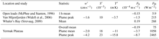
(McPhee and Stanton, 1996)(Widell et al., 2006)(Sirevaag, 2009)Table 1Statistics of fluctuations and turbulent fluxes in the present study over the Yermak Plateau in comparison with other Arctic studies of turbulent heat and salt fluxes.
The impact of drift velocity on the plume observations is investigated in Fig. 6. Drift speed does not relate linearly with the maximal heat flux in the plumes. In fact, many of the most intense plumes observed (highest FH) are during weak or moderate current speed. The peak in vertical velocity increases with increasing current speed (Fig. 6b). This does not imply that plumes are stronger during fast drift, but rather that wmax is dominated by increasingly large turbulent eddies. Stronger turbulence causes more efficient entrainment of ambient water into the plumes, leading to a lower peak in turbulent heat flux. Drift speed also relates to the deviation in temperature from freezing, ΔT = T − Tf, calculated from mean SA and Φ over the 14 s surrounding the peak in vertical velocity. For low drift speed, many of the plume observations carry water that is supercooled relative to the ambient. The supercooling is caused by the lower salinity-determined equilibrium temperature of the brine within the sea ice. Supercooling decreases with drift speed and is not observed for plumes in which the mean current exceeds ∼ 25 cm s−1, which is consistent with stronger mixing of the plumes during high drift speed. Plumes associated with high maximum heat fluxes are more often supercooled than not.
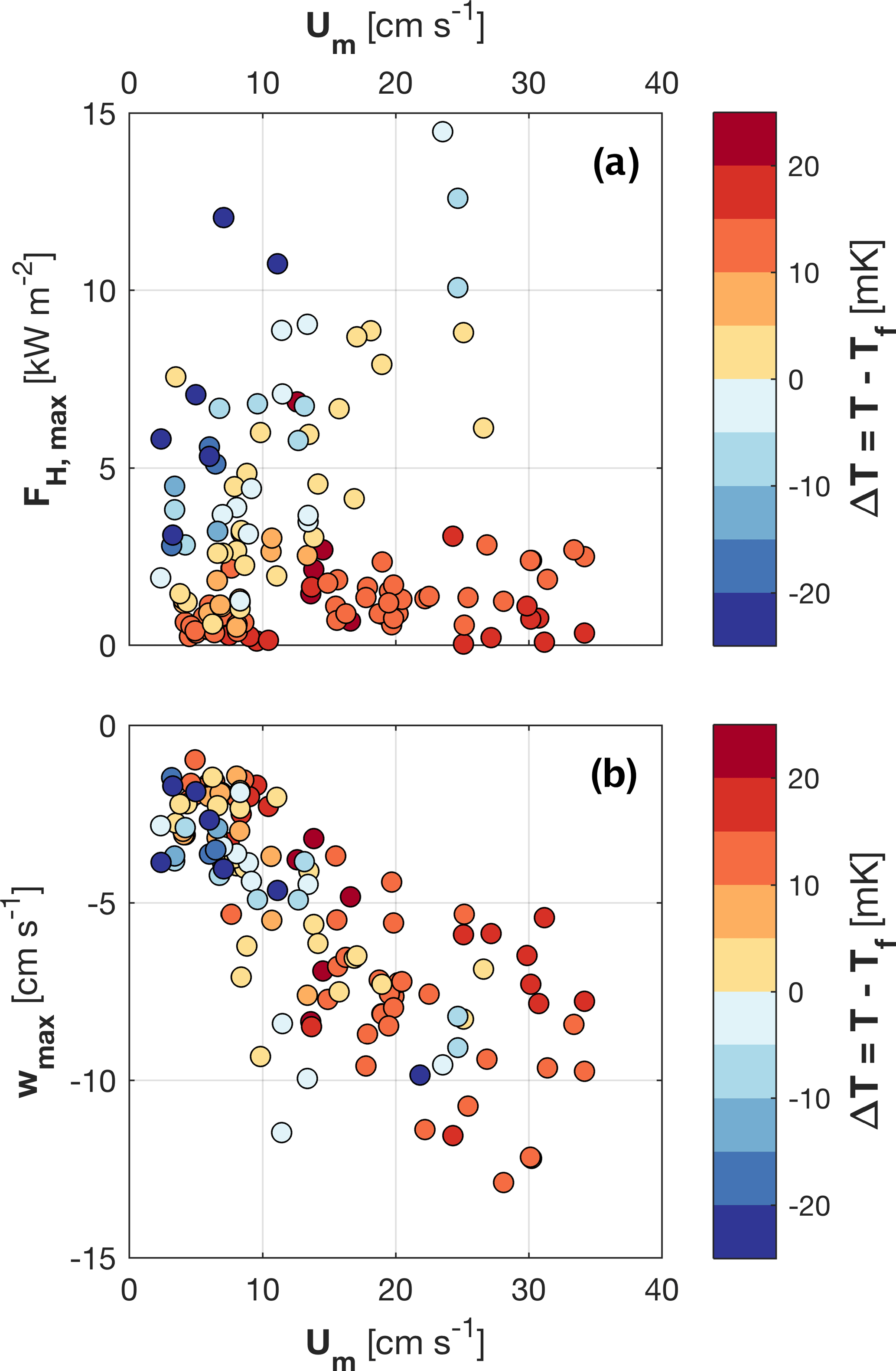
Figure 6Mean horizontal current (Um) vs. instantaneous (a) maximum heat flux and (b) minimum vertical current speed. Circles are color coded for temperature above freezing (ΔT = T − Tf), calculated using mean absolute salinity and conservative temperature (McDougall and Barker, 2011). Mean values are calculated over the 14 s surrounding the peak vertical current speed of each identified plume.
The accumulated salt release during the flux observations was 7.6 kg m−2 summed over available measurements between 11 and 19 June (Fig. 2b). This is equivalent to a salinity decrease of 5 for 1.5 m thick ice. The salt flux observed here is approximately equivalent to the total salt content of the 13 June ice core. About half of the salt flux was observed before the ice core was sampled, so desalination had already taken place before coring. The salt flux observed after the time of coring accounts for 57 % of the total salt content of the ice core on 13 June. The salt flux measured between the time of the two cores is 2.8 kg m−2, the same amount as the change in salt content of the two ice cores. However, gaps in the time series point to a discrepancy between ice cores and observed salt flux. Assuming the salt flux during the measurement gaps was equal to the mean of available measurements, the accumulated salt flux between the two ice cores is approximately twice the observed reduction in the ice cores. The discrepancy might be linked to spatial inhomogeneity in ice composition and melt rates, variability between individual ice cores, or measurement errors (Sect. 6). Agreement between measured fluxes and salinity in ice cores within a factor of 2 supports the fact that the salt flux can originate in brine release from the sea ice.
Calculated over the 14 s surrounding the peak salinity flux in the mean plume structure, the 131 identified events account for 0.7 m s−1, or 9 %, of the observed total salt release within a duration of 31 min (0.5 % of the time), illustrating the intensity of the events. The heat flux averaged over the composite plume is 1058 W m−2, and the plumes account for 6 % (4.7 W m−2) of the average observed heat flux between noon on 11 June and the end of measurements on 19 June. However, the plumes can additionally cause mixing of the surface layers, which could counteract the stabilizing effects of bottom melt. The overall effect of the plumes on heat fluxes is thus difficult to quantify. Upper ocean hydrography profiles (Meyer et al., 2016) do not provide conclusive evidence, as advection and mixed layer deepening from wind forcing obscures any effect from the plumes.
Percolation or flushing of melt ponds could influence the measurements. Although the first melt pond was noted on 9 June, they remained at a very early stage throughout the measurement period reported here. The pond fraction reached an estimated 10 % coverage. Mostly, ponds had formed at deformation areas where freeboard was negative and were thus flooded with seawater rather than actual being melt ponds (A. Rösel, personal communication, 14 January 2017). Salinity measurements from three melt ponds revealed an absolute salinity of 20–29 g kg−1 (Shestov, 2017). The ice core from 13 June (Fig. 4) had a 2 cm negative freeboard, and the deepest snow layer had a salinity of 4.3. Based on this and noting the high permeability of the ice (high liquid fraction; Fig. 4c), percolation may have played a role in the desalination process, but is not pursued further here.
The combined heat flux from above and below finally melted the sea ice. Substantial melt is also evident from the different ice thickness measurements (Fig. 2a). At the end of the flux measurements there were only a few decimeters of ice left, and the floe disintegrated as the instruments were recovered on 19 June. Over the course of the measurements, bottom melt caused an overall reduction in salinity measured at 1 m by approximately 1.
The observations of saline plumes presented here extend the findings of Widell et al. (2006) and are the first observations of such plumes from drifting Arctic sea ice. While the structure is similar to the observations from Van Mijenfjorden (Widell et al., 2006), which were made with the same instrumentation on landfast ice, the magnitudes observed here are much greater, with peak values of salt and heat fluxes in the average plume of FS = −8.7 × 10⁻⁴ m s−1 and FH = 2465 W m−2 (see Table 1). While the measurements by Widell et al. (2006) were made during little (or no) ice melt, the present observations were made during severe melting, which may be the primary difference between the two studies. The fjord study concluded that oceanic heat from the tidal inflow likely triggered brine release from the temperate ice (Widell et al., 2006).
During melting conditions, desalination can happen by gravity drainage or flushing (Notz and Worster, 2009). Flushing can occur when there is an overhead pressure from meltwater at the surface. The negative freeboard in the ice core and saline melt ponds indicate that there was in fact overhead seawater at the surface, which may have caused or at least increased desalination.
Gravity drainage occurs when the buoyancy of the brine exceeds the dissipative effects of thermal diffusion and viscosity within the sea ice. Atmospheric cooling in winter causes higher brine salinity and thus density in the upper part of the ice column. This makes the brine unstable, and convection within the ice takes place when the ice is sufficiently permeable (Notz and Worster, 2009). As the ice warms in spring, permeability increases as illustrated in Fig. 7. The brine fraction in the ice cores exceeds 10 % throughout the ice (Fig. 4c), both well above the typical 5 % threshold required for gravity drainage (Cox and Weeks, 1975). The instability needed for full-depth brine convection in the ice can be triggered by atmospheric or oceanic heat or a combination of the two (Griewank and Notz, 2013). The temperature at the ice–ocean interface is always at its salinity-determined freezing point, and warming from below can only be caused by freshening at the interface by ice melt.
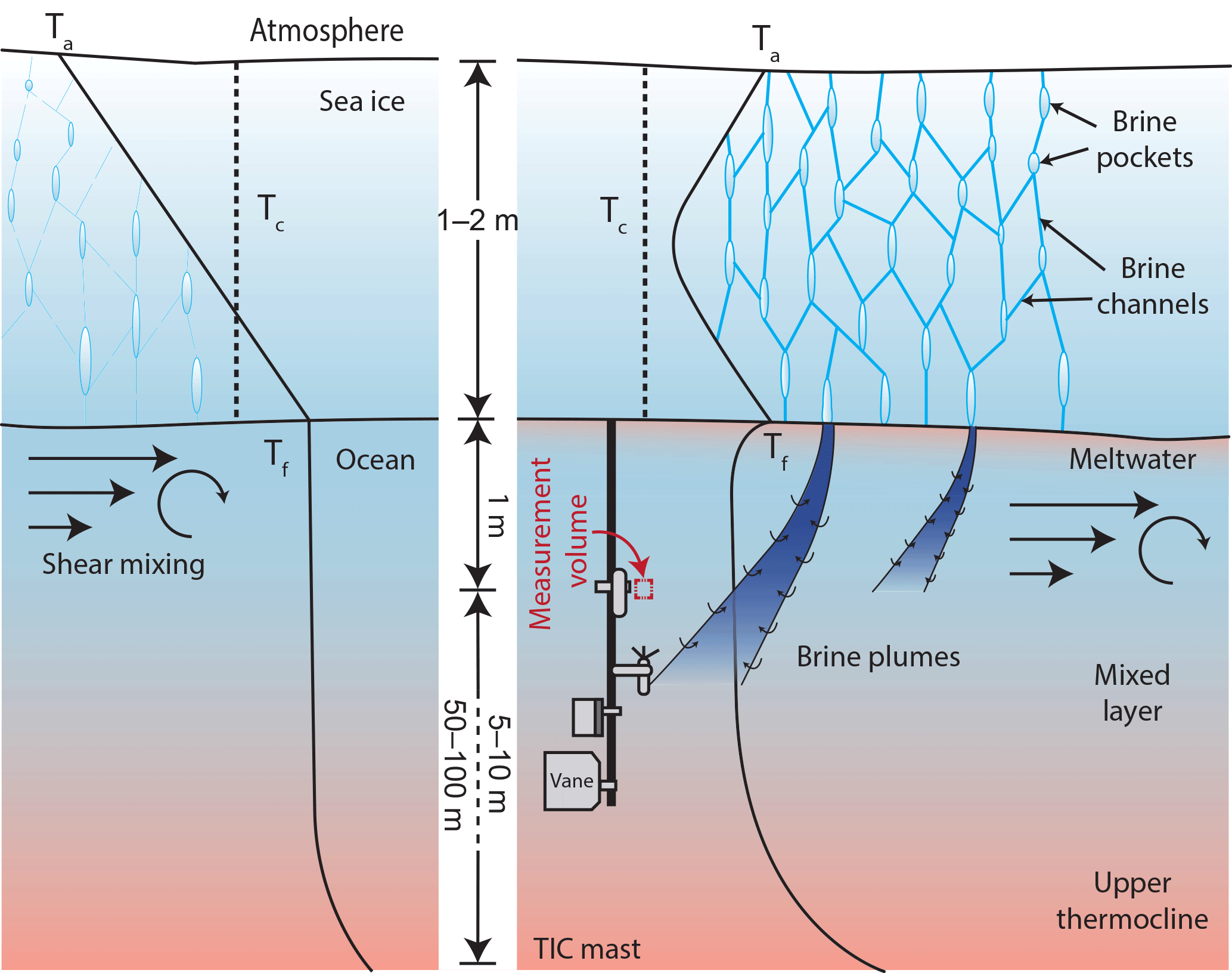
Figure 7To the left is an early spring situation in which the upper ocean is near freezing, and temperature in the ice is still below the critical temperature Tc, which must be exceeded for gravity drainage to occur. When the atmosphere warms the ice, permeability of the sea ice increases, and gravity drainage can occur. The brine plumes are triggered by meltwater below the ice, by directly exposing brine pockets, or by elevating the freezing point temperature Tf at the interface. The TIC mast is shown for reference, with measurement volume at 1 m below the ice.
Ice melts at the ocean interface when the heat supplied by the ocean exceeds the conductive heat flux in the ice. The high oceanic heat fluxes are caused by a combination of the passing storm, the presence of warm Atlantic water near the surface, and the high mobility of the sea ice driving mixing (Meyer et al., 2017b; Peterson et al., 2017); this accounts for much of the observed melt. As the interface freshens, the interface's salinity-determined temperature Tf(S) increases (Fig. 7). Tf remains high as long as the fresh water is allowed to remain at the interface, or enough new meltwater is supplied. Additionally, fresh water supplied by melting at the ice–ocean boundary increases the density deficit between the lower part of the ice and of the brine, which may increase the potential for gravity drainage.
The various ice thickness data (Fig. 2a) show that significant melt was indeed occurring, up to as much as 25 cm day−1 during the observation period. Furthermore, the present observations show positive temperature anomalies prior to the plume events (Fig. 5c). The positive temperature anomaly before the plumes, the sustained positive heat fluxes (Fig. 2a), and the rapid melt suggest that oceanic heat plays a key role through ice melt, as required for triggering repeated convection events.
The difference in salt content between the two ice cores is mostly (∼ 75 %) due to a reduction in ice thickness. The rapid ice melt is thus the cause of most of the salt release and likely the reason for the large difference between values observed here and those of Widell et al. (2006), in which little or no ice melt took place. In addition to gravity drainage or flushing of brine, the brine pockets become directly exposed as melt progresses and sink past the measurement volume. Considering that most of the ice volume is lost during the measurements, it is not surprising if most of the original brine content in the ice is lost. It is, however, surprising that measurements at 1 m below the ice are of the same order of magnitude as the total desalination, which calls for an investigation of possible measurement errors or biases (Sect. 6).
When sea ice melts, it contributes to a net freshening of the upper ocean, since the bulk salinity is about 5 (Fig. 4). Over the course of the drift, a freshening of the surface layer is observed, while the turbulence measurements at 1 m show negative salt flux. This paradox warrants some consideration of the structure of sea ice. Sea ice consists of freshwater ice surrounding pockets of liquid high-salinity brine. When the sea ice melts, the brine sinks through the surface layer due to its high density, while the fresh meltwater stays at the surface. The fresh surface water is gradually entrained into the mixed layer, but since the salt flux is nearly always negative, this freshwater flux likely occurs on timescales longer than the 15 min segments used here. Why fresh water at the surface is not immediately mixed down, even during quite strong mixing events, is not entirely clear. The ice floe consists of first-year ice (Granskog et al., 2017), but the floe was deformed through several storms. This is evident, for example, from the hot wire measurements, which were made in an area of deformed ice. A rough undersurface of the sea ice leads to a thicker layer in which molecular viscosity and diffusivity are important. This “transitional sublayer” is usually taken as 1∕30 of the scale of the roughness elements and is on the scale of a few centimeters (McPhee, 2017).
Since the salt flux observed within the 131 identified plumes only accounts for 9 % of the total salt flux, most of the salt flux takes place outside these plumes. Many more plumes are likely present nearby, but do not reach or cross the measurement volume. Such plumes would bring higher-salinity water somewhere above the TIC, rather than being immediately mixed in with the fresh water at the ice–ocean interface. Subsequent mixing would be observed as a negative salt flux, although not identified as a plume. This may be the reason why salt fluxes are consistently negative, even though direct plume observations are more sporadic.
Brine released from sea ice would initially be at its salinity-determined freezing point in balance with the surrounding ice. As the brine descends from the ice, it may thus be supercooled relative to its surroundings. When the horizontal velocity (and u*) is greater, shear mixes and dilutes the released salt plumes more than during calm conditions. This is consistent with the observation of less supercooling with higher mean current, as seen in Fig. 6. Maximum vertical velocity in the plumes coincided with higher drift speed, which is likely caused by stronger turbulent eddies. The individual plumes do not grow more intense with stronger turbulence, but are more efficiently mixed into the surroundings.
The observations of brine plumes raise interesting questions concerning the conditions in which they occur and, importantly, why they have not been observed before. Few studies have reported measurements of turbulent salt fluxes in the Arctic Ocean, and the season of the observations may be of the essence. In the preceding ice camp (Floe 3) in the N-ICE campaign, the salt fluxes were below the sensor accuracy level and could not be analyzed for correlation with heat flux. The study by Sirevaag (2009) is relevant for comparison because it was set in roughly the same place, Whaler's Bay, in April 2003. The differences between this study and Sirevaag (2009) may give some clues to the matter. They deployed the TIC in a refrozen lead surrounded by ridged multi-year sea ice. An ice core revealed a linear temperature gradient of −21.7 K m−1, meaning that the ice was not above the critical 5 % threshold for gravity drainage. The cold ice column may explain why brine was prevented from leaving the sea ice in plumes, despite rapid melt. When brine is released slowly as melt progresses, it is more likely to be mixed in with meltwater than to descend in plumes.
Salinity is calculated from a Sea-Bird Electronics SBE 4 conductivity cell. The dependence of salinity on both conductivity and temperature can introduce spurious salt fluxes because of a difference in response time between the temperature sensor and the conductivity cell. The standard SBE 4 was chosen for flux calculations rather than the SBE 7 micro-conductivity sensor because the SBE 7 reported suspicious values for part of the record. McPhee and Stanton (1996) made a comparison of a ducted conductivity cell (SBE 4) with a fast-response micro-conductivity sensor (SBE 7) and showed that most of the covariance occurred at lower frequencies. About 75 % of the salinity flux was resolved by the SBE 4. The present observations are obtained during moderate to strong forcing (5–35 cm s−1 drift speed), which improves the response time of the conductivity cell. It is advisable to interpret the observed fluxes with this uncertainty in mind, but note that the fluxes from the ducted conductivity are more likely an underestimate than an overestimate.
Considering the possibility of a baroclinic signal from the edge of the ice floe contaminating the measurements, the vertical modal structure is calculated from the profiles of buoyancy frequency shown in Fig. 3b. The phase velocity of the first baroclinic vertical mode is 0.25–0.43 m s−1 for the four profiles. Taking the closest distance to the floe edge of ∼ 200 m, this implies a timescale for a signal originating at the floe edge of around 10 min. This is comparable to the segment length used for flux calculations (15 min), which could violate the validity of Taylor's hypothesis here. However, the systematic quality control described in Sect. 2 was designed to identify any violation of Taylor's hypothesis and would thus have been excluded from the analysis.
Increased buoyancy frequency during the summer drift could affect the flux measurements. While the typical buoyancy period was about 1 h for the most of the drift (January through May), periods around 10 min or less were seen in June. Oscillations with periods on the order of the 15 min segment length could affect turbulent fluxes. However, recalculating the data set using 5 min segments revealed no significant differences, and Peterson et al. (2017) concluded that the systematic quality control had already flagged any contaminated segments.
The hydrohole, through which the turbulence mast is deployed, can be suspected to affect measurements, and lateral heating may have caused faster melt in some radius around the hole. Still, the horizontal component of the flow is larger than the vertical, and observations made at the TIC represent conditions at the ice interface some distance away. Taking a vertical velocity anomaly of 2–5 cm s−1 and the mean horizontal component of ΔU ∼ 10 cm s−1 (difference between drift velocity and current measured at 1 m; Fig. 2), a plume signal moves 2–5 m in the horizontal over the 1 m vertical distance from the ice–ocean interface. The swiftest vertical speeds are also typically associated with large horizontal speed (Fig. 6). This indicates that even for the large vertical speed seen in the plumes, influence from processes around the hydrohole is typically not expected.
The exact distance between the TIC measurement volume and the ice undersurface may be important for the absolute values observed, as one would expect plumes to gradually expand in size but weaken in terms of buoyancy anomaly with distance from the ice. The manual measurements of ice thickness are accompanied by adjustments of the instrument depth. After each ice thickness measurement, the instrument was elevated to account for the ice melt. Interpreted from notes on these adjustments, the measurement volume was always at the correct depth within the range of the measurement uncertainty. In Fig. 2a, the uncertainty is arbitrarily set to ±15 cm.
Overall, salinity decreases by about 1 over the course of the drift, as measured by the instrument at 1 m. At the same time, the accumulated salt flux accounts for an increase in salinity of 1.7 if distributed over the 4.7 m average mixed layer depth (Meyer et al., 2017b). The apparent inconsistency is caused by the separation in timescales. Over longer timescales, fresh water from ice melt is fluxed downwards, but is not apparent in the turbulence record because each 15 min segment is detrended before fluxes are calculated. The comparison between accumulated salt flux and the salt contents of the ice core indicates that most of the brine in the ice convects down past the surface layer, rather than blending in with the fresh meltwater at the interface. Thus, it appears that brine plumes as observed here affect the timing of the salt release, alter how the salt from sea ice is distributed in the water column, and can be an important factor influencing mixing during sea ice melt.
This study reports observations of inversely correlated heat and salt fluxes below melting sea ice north of Svalbard. The evidence suggests that the fluxes are caused by brine release from the sea ice as it melts, and a significant fraction of the salt fluxes are seen descending past the measurement volume in plumes. Desalination of sea ice similar to that observed here likely occurs in the MIZ in spring in general, when enough heat is present to trigger such events. The present desalination appears to be forced by a combination of flushing, gravity drainage, and direct release of salt through rapid melt caused by oceanic heat flux. Triggering by ocean heat flux is less likely in the Arctic interior, both because there is typically less heat available to be mixed up (e.g., less open water to be warmed by insolation) and less mixing due to internal forces in the pack ice. In the interior Arctic Ocean, sea ice is typically second- or multi-year ice, which is thicker and less saline than first-year ice. Brine release in the quantities reported here are thus more likely a MIZ phenomenon. With the transition towards a more seasonal ice cover in the Arctic, the fraction of first-year ice is increasing (Meier et al., 2014). First-year ice is more saline (Petrich and Eicken, 2010), with an equivalently greater potential for brine drainage. While this could indicate that saline first-year ice can melt faster than fresher multi-year ice in otherwise similar conditions, the transition to more FYI comes with increased freshwater runoff and increased upper ocean stratification (Nummelin et al., 2016). Desalination appears to be a significant process in sea ice melt, although small in comparison to frontal processes and solar heating. Understanding desalination processes may still be increasingly more important in the “new Arctic” and requires more targeted field campaigns.
The following data sets are used in this study and are publicly available at the Norwegian Polar Data Centre: turbulence instrument cluster data (Peterson et al., 2016), microstructure sonde (MSS) profiles (Meyer et al., 2016), meteorological data (Hudson et al., 2015), ice thickness from hot wires (Rösel et al., 2016), and ice core data (Gerland et al., 2017).
The author declares no conflict of interest.
The fieldwork has been supported by the Norwegian Polar Institute's Centre
for Ice, Climate and Ecosystems (ICE) through the N-ICE project. The author
would like to thank everyone involved in the fieldwork, and Amelie Meyer in
particular, for keeping the instruments going until the very end. Thanks to
Ilker Fer, Dirk Notz, Mats Granskog, Martin Vancoppenolle, Craig Stevens, and
the anonymous reviewers for useful discussions and input and to Miles McPhee
for making the instrumentation available. The author is supported by the
Research Council of Norway through project 229786, with additional
support from the Centre for Climate Dynamics at the Bjerknes Centre through
the grant BASIC: Boundary Layers in the Arctic Atmosphere, Seas and Ice Dynamics.
Edited by: Eric J. M. Delhez
Reviewed by: Craig Stevens and one anonymous referee
Carmack, E. C., Polyakov, I. V., Padman, L., Fer, I., Hunke, E., Hutchings, J. K., Jackson, J., Kelley, D. E., Kwok, R., Layton, C., Melling, H., Perovich, D. K., Persson, O., Ruddick, B., Timmermans, M.-L. L., Toole, J. M., Ross, T., Vavrus, S., and Winsor, P.: Toward quantifying the increasing role of oceanic heat in sea ice loss in the new Arctic, B. Am. Meteorol. Soc., 96, 2079–2105, https://doi.org/10.1175/BAMS-D-13-00177.1, 2015. a
Cohen, L., Hudson, S. R., Walden, V. P., Graham, R. M., and Granskog, M. A.: Meteorological conditions in a thinner Arctic sea ice regime from winter to summer during the Norwegian Young sea ice expedition (N-ICE2015), J. Geophys. Res., 122, 7235–7259, https://doi.org/10.1002/2016JD026034, 2017. a, b, c
Cox, G. F. N. and Weeks, W. F.: Brine drainage and initial salt entrapment in sodium chloride ice, CRREL Research Report, CRREL, Hanover, NH, 1975. a, b
Emery, W. J. and Thomson, R. E.: Data analysis methods in physical oceanography, 2nd Edn., Elsevier, Amsterdam, the Netherlands, 2001. a
Gerland, S., Granskog, M. A., King, J., and Rösel, A.: N-ICE2015 ice core physics: temperature, salinity and density [Data set], https://doi.org/10.21334/npolar.2017.c3db82e3, 2017. a
Golden, K. M., Ackley, S. F., and Lytle, V. I.: The percolation phase transition in sea Ice, Science, 282, 2238–2241, https://doi.org/10.1126/science.282.5397.2238, 1998. a
Granskog, M. A., Assmy, P., Gerland, S., Spreen, G., Steen, H., and Smedsrud, L.H.: Arctic research on thin ice: Consequences of Arctic sea ice loss, Eos, 97, https://doi.org/10.1029/2016EO044097, 2016. a, b
Granskog, M. A., Rösel, A., Dodd, P. A., Divine, D. V., Gerland, S., Martama, T., Leng, M. J., Martma, T., and Leng, M. J.: Snow contribution to first-year and second-year Arctic sea ice mass balance north of Svalbard, J. Geophys. Res.-Oceans, 122, 2017–2033, https://doi.org/10.1002/2016JC012398, 2017. a, b, c, d
Griewank, P. J. and Notz, D.: Insights into brine dynamics and sea ice desalination from a 1-D model study of gravity drainage, J. Geophys. Res.-Oceans, 118, 3370–3386, https://doi.org/10.1002/jgrc.20247, 2013. a, b
Hudson, S. R., Cohen, L., and Walden, V.: N-ICE2015 surface meteorology [Data set], https://doi.org/10.21334/npolar.2015.056a61d1, 2015. a, b
Jardon, F. P., Vivier, F., Vancoppenolle, M., Lourenço, A., Bouruet-Aubertot, P., and Cuypers, Y.: Full-depth desalination of warm sea ice, J. Geophys. Res.-Oceans, 118, 435–447, https://doi.org/10.1029/2012JC007962, 2013. a, b
McDougall, T. J. and Barker, P. M.: Getting started with TEOS-10 and the Gibbs Seawater (GSW) Oceanographic Toolbox, SCOR/IAPSO WG, 127, 1–28, 2011. a, b
McPhee, M. G.: Turbulent stress at the ice/ocean interface and bottom surface hydraulic roughness during the SHEBA drift, J. Geophys. Res., 107, 8037, https://doi.org/10.1029/2000JC000633, 2002. a
McPhee, M. G.: The sea ice–ocean boundary layer, in: Sea ice, chap. 5, 3rd Edn., edited by: Thomas, D. N., John Wiley & Sons, Ltd, Oxford, UK, 138–159, 2017. a
McPhee, M. G. and Stanton, T. P.: Internal waves and velocity fine structure in the Arctic Ocean, J. Geophys. Res., 101, 6409–6428, https://doi.org/10.1029/91JC01071, 1996. a, b, c
McPhee, M. G., Maykut, G. A., and Morison, J. H.: Dynamics and thermodynamics of the ice/upper ocean system in the marginal ice zone of the Greenland Sea, J. Geophys. Res., 92, 7017, https://doi.org/10.1029/JC092iC07p07017, 1987. a
McPhee, M. G., Morison, J. H., and Nilsen, F.: Revisiting heat and salt exchange at the ice-ocean interface: Ocean flux and modeling considerations, J. Geophys. Res., 113, C06014, https://doi.org/10.1029/2007JC004383, 2008. a
Meier, W. N., Hovelsrud, G. K., van Oort, B. E., Key, J. R., Kovacs, K. M., Michel, C., Haas, C., Granskog, M. A., Gerland, S., Perovich, D. K., Makshtas, A., and Reist, J. D.: Arctic sea ice in transformation: A review of recent observed changes and impacts on biology and human activity, Rev. Geophys., 52, 185–217, https://doi.org/10.1002/2013RG000431, 2014. a
Meyer, A., Fer, I., Sundfjord, A., Peterson, A. K., Smedsrud, L. H., Muijlwick, M., Randelhoff, A., Håvik, L., Koenig, Z., Onarheim, I. H., Davies, P., Miguet, J., and Kusse-Tiuz, N.: N-ICE2015 ocean microstructure profiles (MSS90L) [Data set], https://doi.org/10.21334/npolar.2016.774bf6ab, 2016. a, b
Meyer, A., Fer, I., Sundfjord, A., and Peterson, A. K.: Mixing rates and vertical heat fluxes north of Svalbard from Arctic winter to spring, J. Geophys. Res.-Oceans, 119, 7123–7138, https://doi.org/10.1002/2016JC012441, 2017a. a
Meyer, A., Sundfjord, A., Fer, I., Provost, C., Villacieros Robineau, N., Koenig, Z., Onarheim, I. H., Smedsrud, L. H., Duarte, P., Dodd, P. A., Graham, R. M., Schmidtko, S., and Kauko, H. M.: Winter to summer oceanographic observations in the Arctic Ocean north of Svalbard, J. Geophys. Res.-Oceans, 122, 6218–6237, https://doi.org/10.1002/2016JC012391, 2017b. a, b, c, d
Notz, D. and Worster, M. G.: Desalination processes of sea ice revisited, J. Geophys. Res.-Oceans, 114, 1–10, https://doi.org/10.1029/2008JC004885, 2009. a, b, c
Notz, D., Wettlaufer, J. S., and Worster, M. G.: A non-destructive method for measuring the salinity and solid fraction of growing sea ice in situ, J. Glaciol., 51, 159–166, https://doi.org/10.3189/172756505781829548, 2005. a
Nummelin, A., Ilicak, M., Li, C., and Smedsrud, L. H.: Consequences of future increased Arctic runoff on Arctic Ocean stratification, circulation, and sea ice cover, J. Geophys. Res.-Oceans, 121, 617–637, https://doi.org/10.1002/2015JC011156, 2016. a
Peterson, A. K., Fer, I., Randelhoff, A., Meyer, A., Håvik, L., Smedsrud, L. H., Onarheim, I. H., Muijlwick, M., Sundfjord, A., and McPhee, M. G.: N-ICE2015 ocean turbulent fluxes from under-ice turbulent cluster [Data set], https://doi.org/10.21334/npolar.2016.ab29f1e2, 2016. a, b
Peterson, A. K., Fer, I., McPhee, M. G., and Randelhoff, A.: Turbulent heat and momentum fluxes in the upper ocean under Arctic sea ice, J. Geophys. Res.-Oceans, 122, 1–18, https://doi.org/10.1002/2016JC012283, 2017. a, b, c, d, e
Petrich, C. and Eicken, H.: Growth, structure and properties of sea ice, in: Sea ice, chap. 2, 2nd Edn., edited by: Thomas, D. N. and Dieckmann, G. S., John Wiley & Sons, Ltd, Oxford, UK, 23–77, 2010. a, b
Rösel, A., Bratrein, M., King, J. A., Itkin, P., Divine, D., Ervik, Å., Gallet, J.-C., Gierisch, A., Haapala, J., Oikkonen, A., Liston, G. E., Nicolaus, M., Polashenski, C. M., Spreen, G., Gerland, S., Granskog, M. A., and Perovich, D. K.: N-ICE2015 ice thickness from hot wires [Data set], https://doi.org/10.21334/npolar.2016.263a317f, 2016. a, b
Shestov, A.: Field report on the Ridge activity during N-ICE2015, Leg 6, Tech. rep., UNIS, Longyearbyen, Norway, 2017. a
Sirevaag, A.: Turbulent exchange coefficients for the ice/ocean interface in case of rapid melting, Geophys. Res. Lett., 36, L04606, https://doi.org/10.1029/2008GL036587, 2009. a, b, c, d, e, f
Turner, J. S.: The melting of ice in the Arctic Ocean: The influence of double-diffusive transport of heat from below, J. Phys. Oceanogr., 40, 249–256, https://doi.org/10.1175/2009JPO4279.1, 2010. a
Widell, K., Fer, I., and Haugan, P. M.: Salt release from warming sea ice, Geophys. Res. Lett., 33, L12501, https://doi.org/10.1029/2006GL026262, 2006. a, b, c, d, e, f, g, h, i, j, k