the Creative Commons Attribution 4.0 License.
the Creative Commons Attribution 4.0 License.
 | 19 Mar 2026
Best practices for estimating turbulent dissipation from oceanic single-point velocity timeseries observations
Cynthia E. Bluteau
Danielle J. Wain
Julia C. Mullarney
Craig L. Stevens
We provide best practices for estimating the dissipation rate of turbulent kinetic energy, ε, from velocity measurements in an oceanographic context. These recommendations were developed as part of the Scientific Committee on Oceanographic Research (SCOR) Working Group #160 “Analyzing ocean turbulence observations to quantify mixing”. The recommendations here focus on velocity measurements that enable fitting the inertial subrange of wavenumber velocity spectra. The method examines the measurable range for this method of dissipation rates in the ocean, seas, and other natural waters. The recommendations are intended to be platform-independent since the velocities may be measured using bottom-mounted platforms, platforms mounted beneath the ice, or platforms directly on mooring lines once the data is motion-decontaminated. The procedure for preparing the data for spectral estimation is discussed in detail, along with the quality control metrics that should accompany each estimate of ε during data archiving. The methods are applied to four “benchmark” datasets covering different flow regimes and two instrument types (acoustic-Doppler and time of travel). Problems associated with velocity data quality, such as phase-wrapping, spikes, measurement noise, and frame interference, are illustrated with examples drawn from the benchmarks. Difficulties in resolving and identifying the inertial subrange are also discussed, and recommendations on how these issues should be identified and flagged during data archiving are provided.
- Article
(7334 KB) - Full-text XML
- BibTeX
- EndNote


Quantifying turbulence and mixing in the ocean is critical for understanding many processes including the turbulent transfer of momentum, heat and material – as well as the dissipation of energy (Fox-Kemper et al., 2019). For example, when seeking to understand how an ocean boundary layer responds to wind, it is critical to reliably understand how energy is dissipated by a turbulent cascade to the viscous scales – or how material is exchanged across isolines, such as the seasonal thermocline, as well as through boundaries of the fluid into the benthos or atmosphere (D'Asaro, 2014). However, owing to the small temporal and spatial scales which inherently characterize turbulent flow, key representative quantities are often not straightforward to measure (Gregg, 1999). The dissipation rate of turbulent kinetic energy ε describes the energy lost from the fluid system to viscous dissipation. In addition, ε can be related to processes that drive turbulent fluxes of momentum, heat and material. The small scales and variable nature of the processes require precise measurement and analysis before one arrives at an estimate of ε and associated quantities.
These computations are especially challenging in the ocean as ε can range over almost ten orders of magnitude (Stewart and Grant, 1999). Consequently, distinct measurement techniques have been developed for differing parts of this wide range of ε. Microstructure shear probes are particularly useful for measuring turbulence profiles in low to medium energy regions of the ocean as these sensors typically resolve the smallest, viscous, turbulence scales (Lueck et al., 2024). Point-velocity sensors are better suited for obtaining timeseries of dissipation rate than shear probes. However, velocity sensors can typically only resolve the larger turbulence length scales, and thus estimating ε is limited to relatively high energy environments.
Acoustic point-measurement instruments – sensors which measure point-velocity timeseries in the ocean – have been deployed since the mid-1990s (Lemmin et al., 1999; Rusello et al., 2006), and are based on either acoustic backscatter (Trowbridge and Elgar, 2001), or time of travel (Henchicks, 2001) approaches. The time of travel instruments, such as Modular Acoustic Velocity Sensor (MAVS), are typically better suited than the acoustic backscatter approach in environments with low concentration of acoustic scatterers or weak currents. These environments are typically associated with low ε. The single-point measurements were found to be especially well-suited to capture ε values within boundary-layers to improve understanding of dynamics and transfer processes (Li et al., 2022); or, in experiments in which the control volume is fixed in space – i.e., the sensor is mounted on the sea bed or a fixed platform (Fig. 1), rather than in open-ocean measurements of ε such as recorded with a falling profiler (Le Boyer et al., 2023).
Technology for acoustic point velocity timeseries measurements has matured over the last decades, with many commercial instruments now well-established (e.g., the Nortek Acoustic Doppler Velocimeter, ADV, and Nobska Modular Acoustic Velocity Sensor, MAVS), resulting in a wide user base of researchers and engineers. In particular, improvements in noise reduction meant that by the late 1990s, data from these instruments were able to be analysed to provide turbulence estimates (e.g., Voulgaris and Trowbridge, 1998; Kim et al., 2000). Previously, such estimates were only undertaken by a small number of groups worldwide with bespoke equipment that was built, maintained, and operated in-house. With this expansion in the user-base comes a need for consistent, or at least comparable, methods to assess data quality and archive datasets. However, currently no standardized methods or guidelines exist for these velocity measurements.
Here, we address this deficit by describing recommendations for best practices for obtaining ε from point velocity measurements. These recommendations were developed through the Scientific Committee on Oceanic Research working group #160 on Analysing ocean Turbulence Observations to quantify MIXing (ATOMIX), specifically the subgroup on point velocities. Our aim was to evaluate various methods for different processing steps and to provide recommendations of the most robust approach for researchers who are new to measuring turbulence in aquatic and oceanic flows. When multiple methods yielded similar results, we recommended the one that was easiest to implement. The working group also created benchmark datasets to help assess and validate algorithms for estimating ε, regardless of programming language. The format of the benchmarks was designed to let researchers test processing workflows at intermediate checkpoints, enabling them to build on our working group’s activities and propose new techniques. Our choice of benchmarks and their format recognizes that alternative methods may yield similar results at the processing checkpoints.
In addition, ATOMIX developed recommendations for two other types of technologies, shear probes (Lueck et al., 2024), and acoustic-Doppler current profilers (McMillan et al., 2026). The ATOMIX approach promotes a consistent variable naming framework, followed by example-based description of guidelines for formatting, processing level, parameter estimation, and quality control. A key result is the provision of final ε estimates for the benchmark datasets to enable researchers to check their own analyses.
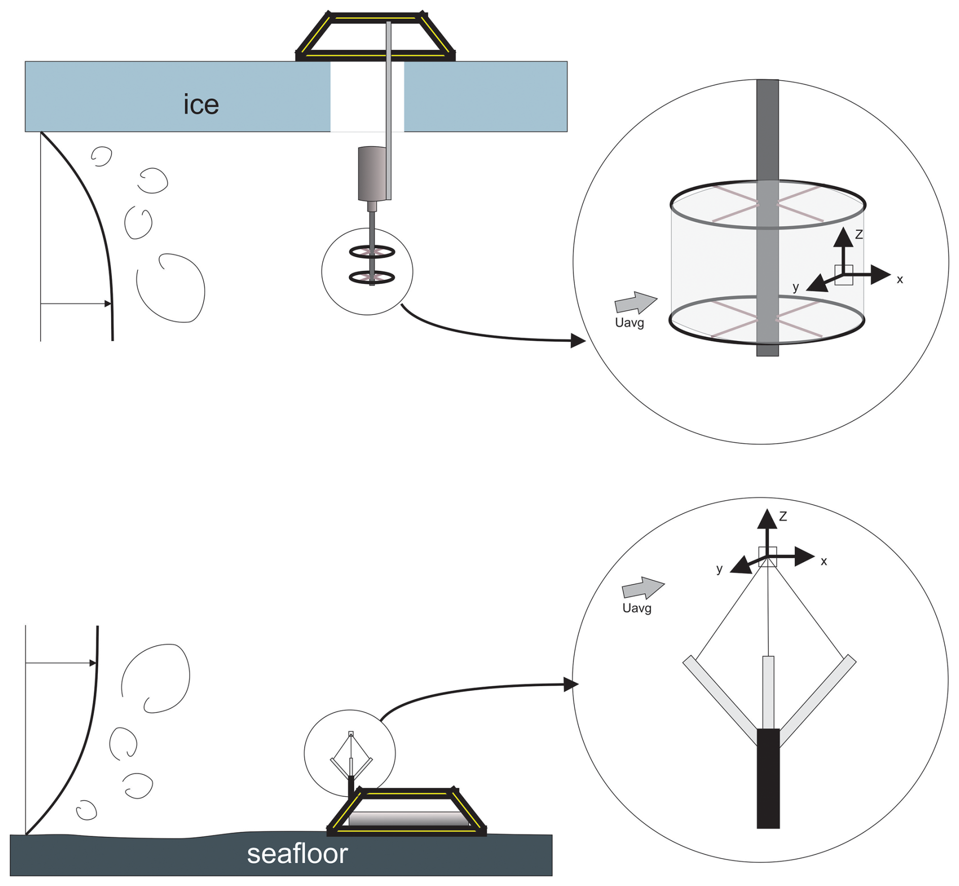
Figure 1Sketch of point velocity deployment configurations showing both under sea ice and seafloor deployments with examples of a time of travel sensor (upper) or acoustic backscatter sensor (lower).
A critical aspect of most approaches to sampling environmental turbulence is that data are typically acquired in the time domain, but the mechanistic, physical understanding is best described and analyzed in the spatial (i.e., wavenumber) domain. Technological developments have reduced the sampling volumes (bin size) measured by current-profilers, thus enabling the direct measurement of spatial spectra (e.g., Shcherbina et al., 2018; Zippel et al., 2021b). However, we focus on the more traditional timeseries measurements that must be converted from temporal to spatial measurements by invoking Taylor's frozen turbulence hypothesis whereby, under certain conditions, turbulent structure can be considered “frozen” as it moves past a stationary sensor (Lumley, 1965; Wyngaard and Clifford, 1977). In practice, this hypothesis requires an estimate of the mean advection speed past the sensor, which enables the conversion of spectral observations from the frequency f (Hz) to wavenumber domain (cpm) as:
The presence of above variables indicate observational or estimated parameters.
Irrespective of whether the instrument is fixed or moving (e.g., drifting or moored), the velocity is always the speed relative to the instrument rather than the actual water speed. This conversion can lead to errors in ε of a few percent when is about ten times larger than the root-mean-square of the turbulent velocity fluctuations in the direction of the mean flow urms (Wyngaard and Clifford, 1977; Lumley, 1965). The error magnitude in flows with low mean speeds was determined more recently by Pécseli and Trulsen (2022), using idealized numerical experiments. Their work excludes the impact of surface waves on the advection of turbulence and the estimated urms. They found that the expected errors on drops when the ratio increases. When was three times larger than urms, the estimates were overpredicted by less than 10 %. The errors grew to about 25 % when was comparable in magnitude to urms (Pécseli and Trulsen, 2022).
Taylor's hypothesis impacts which wavenumbers are resolved in the final spectra. Slower mean speeds enable resolution of the smaller turbulence scales within the viscous subrange without increasing the sampling rate of measurements (Fig. 2). Hence, the expected mean speed must be considered when selecting the sampling frequency of measurements and setting the ambiguity velocity of the instrument. The ambiguity velocity defines the maximum (unambiguous) along-beam velocity that can be measured (for a given transmit pulse). A smaller ambiguity velocity in pulse-coherent Doppler instruments improves the data quality by reducing the measurement noise but might “phase wrap” the measured velocities (Lhermitte and Serafin, 1984; Lohrmann and Nylund, 2008). Section 4.1 covers how phase-wrapped data can be identified and remedied, while the metrics for assessing the validity of Taylor's hypothesis will be discussed in Sect. 4.2.
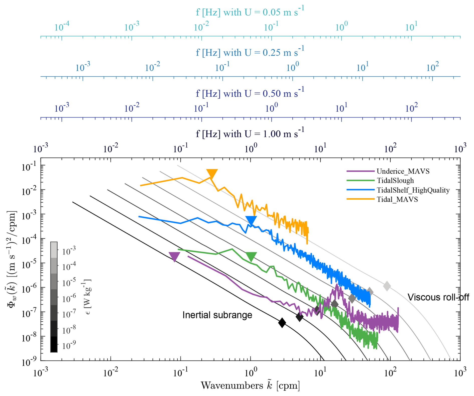
Figure 2Spectral representations from the four benchmark datasets overlaying the expected idealized curves for a range of ε. The secondary frequency axes above the figure shows the relationship between different mean advection speeds and wavenumbers. The gray diamonds denote the empirical limit of the inertial subrange and depend on ε. The coloured triangles represent the approximate distance of the platform from the nearest boundary . The impact of vortex shedding is apparent in the under-ice MAVS example at approximately 25 cpm.
The sampling rate and segmenting choices must consider the time and length scales associated with ocean turbulence, particularly those corresponding to the inertial subrange (Fig. 2). Estimating turbulence quantities from field measurements also necessitates satisfying the stationarity assumption. This assumption implies that the key statistical properties of the flow do not change over timescales shorter than the segment length chosen to estimate ε. This length must also be sufficiently long to resolve the inertial subrange and fit the spectra and obtain ε (see Sect. 4.2). Within the inertial subrange, the cascade of turbulent kinetic energy is independent of both the properties of the mean flow and molecular viscosity (Pope, 2000), unlike the larger scales in the energy-containing range and the smaller scales in the viscous subrange.
The inertial subrange spectral model Ψj(k) is given by:
where k is the wavenumber expressed in rad m−1 rather than expressed in cpm (), Ck is the empirical Kolmogorov universal constant that is approximately Ck=1.5 as given in Sreenivasan (1995). The constant aj depends on the velocity component for estimating ε. In the longitudinal direction , while the values are larger in the vertical and transverse directions, i.e. (Pope, 2000). Sreenivasan (1995) collated and interpreted multiple studies to obtain an average value for Ck = 1.62 (a1Ck = 0.53) with a standard deviation of 0.1681 (or 0.055 for a1Ck).
The inertial subrange covers larger scales than the viscous subrange. It can be nonexistent in low Reynolds number flow in which the larger turbulent scales become more comparable in size to the smallest scales (Saddoughi and Veeravalli, 1994; Gargett et al., 1984). The largest scales depend on the sought-after quantities – ε and the background flow properties, while the smallest scales are defined by the Kolmogorov length scale LK:
where ν is the kinematic viscosity of seawater. The largest wavenumbers of the inertial subrange are about ten times the Kolmogorov scale, which translates to:
(Pope, 2000). When the ratio between the largest and smallest turbulent length scale becomes smaller than roughly 300, the inertial subrange becomes severely anisotropic (see the review in Bluteau et al., 2011). Energy levels drop below those predicted by the isotropic model in Eq. (2), and the inertial subrange becomes unsuitable for estimating ε. These problems typically occur for weakly turbulent flows, especially near boundaries or in highly stratified-sheared flows (Gargett et al., 1984; Saddoughi and Veeravalli, 1994).
Several relationships exist to define the scale of the largest turbulent overturns (Ivey et al., 2018). We provide a brief overview, noting that these scales can be of the order of meters. The scales are always limited by the distance to the nearest boundary, either the bottom or the surface. One common definition for the large overturns in a stratified-sheared flow is the Ozmidov length scale LO (Ozmidov, 1965):
or by the Corrsin length scales in sheared flows (Corrsin, 1958):
where N and S are the background stratification and velocity shear. This length scale tends to be smaller than LO and better represents the low wavenumber limit of the inertial subrange (see, for example Bluteau et al., 2011).
Near boundaries, other definitions for the largest overturn size may be warranted. For example, the Obukhov length scale for ocean convection includes the effects of buoyancy and applied wind stress (Obukhov, 1946; Zheng et al., 2021). Near a solid boundary,
when the assumptions of the log-law of the wall are satisfied (Bluteau et al., 2011). The Von Kàrmàn's constant is κ=0.39, as revised by Marusic et al. (2013) using atmospheric and laboratory observations over a wide range of Reynolds numbers. Hence, when no velocity shear measurements are available, the distance of the nearest boundary can be used to characterize the largest overturns, although this approach may overestimate the overturn sizes (Bluteau et al., 2011).
Generally, the inertial subrange can be identified directly from the spectral observations. Knowledge of the above length scales is important to ensure the sampling and analysis strategies do not inadvertently reduce the range of wavenumbers resolved within the inertial subrange. These scales partly dictate the segmenting and spectral averaging strategies described below (Sect. 4.2 and 4.3), as well as the choice of burst sampling duration if continuous sampling is unfeasible with the available battery power of the instrument.
Measurement campaigns must ensure the sampling rate is sufficiently fast to resolve the high, most isotropic, wavenumbers of the inertial subrange (Fig. 2). The sampling rate must be faster for fast-moving flows than in low-energy environments, although the high-energy flows typically lead to a wider inertial subrange. A sampling rate of 64 Hz has a Nyquist frequency of 32 Hz. If the noise levels are low, the highest wavenumbers of the inertial subrange are resolved for W kg−1 and mean speeds m s−1. For slower expected speeds m s−1, a sampling rate of about 16 Hz suffices for resolving the entire inertial subrange when W kg−1. The sampling rate can be further reduced if the expected ε is much lower than 10−5 W kg−1 (see Fig. 2). However, the noise floor adversely impacts our ability to estimate low ε by potentially drowning out the high wavenumbers of the inertial subrange (Sect. 4.4.3).
The benchmark datasets were created to allow testing of algorithms (independent of programming language) for estimating ε; these datasets cover a range of instrument types and environmental conditions that can be encountered ranging from low-energy environments, such as beneath sea ice or lakes, to high-energy environments, such as sills and obstacles in coastal oceans or shallow embayments and estuaries (Bluteau et al., 2025). Here, we focus on four benchmark datasets encompassing a range of water depths and background flow speeds (Table 1). Other datasets were considered, but the present ones have problematic sections that allowed us to demonstrate the application of quality control metrics.
Table 1Summary of setup, environmental conditions, and estimated for benchmark datasets (Bluteau et al., 2025). The 2.5th, 50th and 97.5th percentiles for mean speed are listed, while the range for represents the 2.5th to 97.5th percentile.
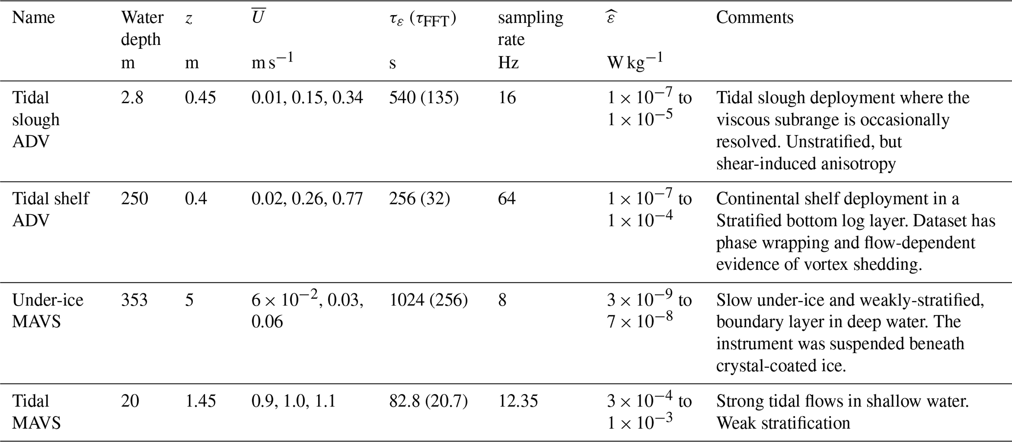
All four datasets are characterized by being recorded relatively close to a horizontal boundary. The four benchmark datasets are split evenly across two types of instruments – (i) acoustic-Doppler velocimeter (ADV) which is a backscatter device, and (ii) Modular Acoustic Velocity Sensor (MAVS) which is a time-of-travel device. The ADV datasets presented here were both collected with a Vector, Nortek AS, while the MAVS instruments were produced by Nobska. The MAVS instrument notably does not require particulate material in the water column to resolve speed fluctuations and, thus, turbulence. However, as we discuss later, their sampling rings shed vortexes that contaminate velocities in the direction perpendicular to the instrument's main shaft (Hay et al., 2013). Bottom frames may also contaminate MAVS and ADV velocity measurements.
We specify the technology type used for collecting the velocities in the names of the benchmark datasets, which can be summarized as follows:
-
Tidal Slough ADV – unstratified, shallow water;
-
Tidal Shelf ADV – stratified boundary-layer with relatively fast speeds, in deep water;
-
Under-ice MAVS – weak flows, 5 m beneath rough ice;
-
Tidal MAVS – fast flows, near bed in shallow and unstratified waters.
The benchmarks use the NetCDF-4 file format with four distinct processing levels stored in their own group named according to the processing level (Fig. 3 and Appendix A). This format was devised to facilitate testing from different checkpoints. Below, in Sect. 4, we explain the processing steps at each level in detail. The first data level contains the raw velocity measurements and boolean quality-control indicators that flag poor-quality velocity samples. The second level involves applying the quality control flags, replacing the missing samples, and then segmenting the time series into smaller subsets, usually a few minutes long. This second level separates each subset of velocity samples used for computing spectra and other statistics required for converting from time to space and for applying the inertial model to the spectra (e.g., mean speed past the sensor).
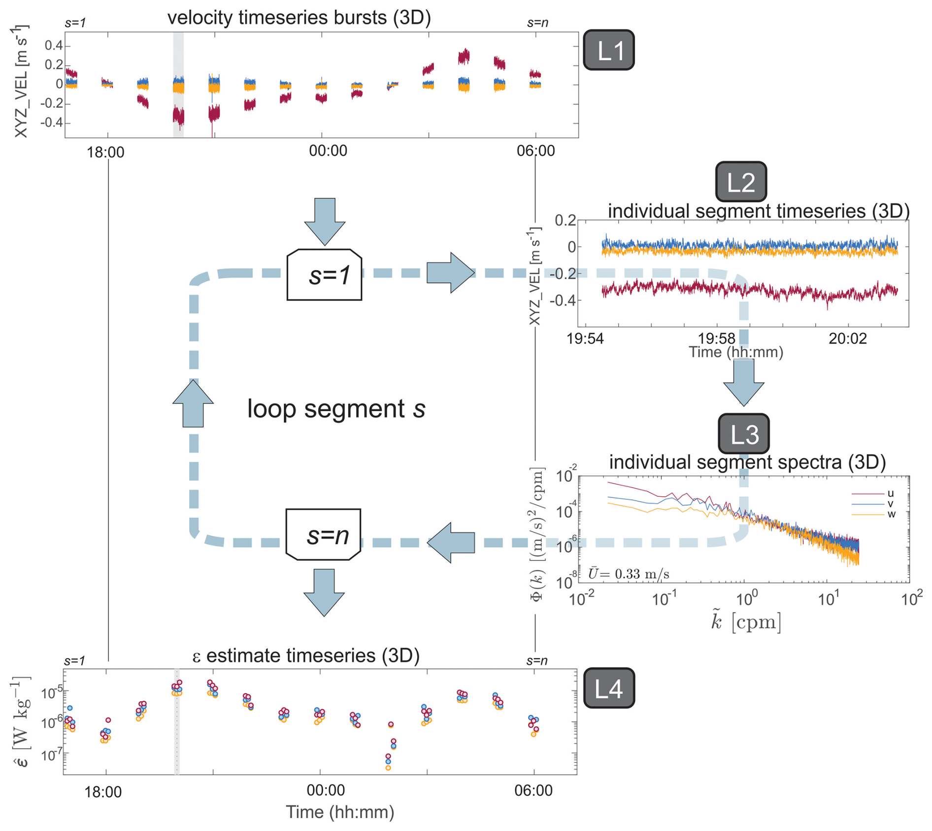
Figure 3Left shows the data processing workflow associated with hierarchical group stored in the NetCDF files. Level 1 begins with the raw timeseries and its quality control flags that get segmented and stored at level 2. These segmented timeseries are converted into spectra at level 3 so that the ε can be estimated to create the final timeseries at level 4.
The third level contains the spectral observations for each segment that are used to derive ε by fitting the observations over the inertial subrange with the appropriate theoretical model (e.g., Eq. 2). The fourth level contains the estimated ε from all available velocity components, along with boolean quality-control flags that indicate one or many reasons why an ε should be discarded or, at the very least, have the quality questioned. The flags' metadata includes thresholds for any quality-control test applied to the original measurements. This level contains the ε, and quality-control indicators, which would typically be presented in a scientific article or technical report.
We detail the best practices for the processing step as they are applied to each NetCDF data level (Fig. 3). Our processing choices were determined using the existing literature, ATOMIX members' experience, and testing of alternative methods. The current benchmarks and proposed best practices are a starting point for eventual processing standards for estimating ε. Our intention is for future users to verify their results at different data processing checkpoints, allowing the quality of archived datasets to improve further over time.
4.1 Quality control of raw velocity measurements
A timeseries, recorded from one instrument, is stored as a two-dimensional matrix where each column represents a velocity component. The Level 1 flags are obtained by applying multiple quality-control processing steps to the raw measurements. We note that several of the quality control steps are applied to the velocities collected in beam coordinates. However, in acoustic systems with three or four transducers, data is rotated into horizontal and vertical velocity components by applying linear transformations to the data in beam coordinates; thus, a “bad data” flag in beam coordinates should generally also be applied when transformed into the xyz coordinates. Below, we describe identification of bad data and formation of the quality control flags as applied to the ADV benchmarks. The MAVS benchmarks have flags only at Level 4 for the estimates. The primary data quality issue for this instrument is vortex shedding from the sampling rings.
4.1.1 Removal of low quality data
The most common indicators of low-quality data are either low backscatter amplitudes or low signal-to-noise ratios, which express the strength of the signal relative to a background noise level (). Critical cut-off values for discarding data are instrument- and environment-specific. For the Nortek Vector used in the benchmark datasets, the manufacturer recommends values are 6 dB above the noise floor (around 50 dB) and 15 for amplitude and SNR, respectively (Nortek, 2018). In contrast, an obstruction of an acoustic beam may manifest as high values in both backscatter and SNR. This obstruction may be identified by a large difference in amplitude between the adjacent acoustic beams, especially if another beam is obstructed.
ADV systems use pulse-to-pulse coherent technology in which a pair of pulses separated by a known time lag are emitted. The similarity between the measured echo of the two pulses is assessed and reported as a percentage value, which provides a further indication of data quality (Lohrmann and Nylund, 2008). It is worth noting that coherence and amplitude are functions of different parameters with varying sensitives, and thus provide two separate measures of quality control. Low correlation values can be used to identify bad data; but the converse is not necessarily true, that is, a large value doesn't indicate good quality data in all cases. A canonical cut-off value of 70 % has been shown to generally reduce variance within the dataset; however, values of 50 % are also commonly used as a cut-off.
Our quality control data format provides users with the ability to specify the threshold and rationale in the NetCDF data file, which should also be described in the methods of their scientific publications. We recommend that these additional user-defined flags also consider other data quality concerns, e.g., the pressure sensor indicating that the instrument was out of the water or change in pitch, roll, or heading indicating that the instrument has moved. Once bad data has been flagged, other QC measures such as phase unwrapping and velocity despiking can be applied to improve data quality.
4.1.2 Phase unwrapping
For pulse-coherent instruments, the Doppler phase shift can only be determined from −π to π. For values outside this range, when the along-beam velocity exceeds the ambiguity velocity as set by the time-lag between pulses, “phase wrapping” can occur. This effect manifests as a sudden and unrealistic change in velocities, which is usually also accompanied by a change in sign. These “phase-wrapped” velocities can sometimes be corrected for in beam coordinates by subtracting or adding twice the ambiguity velocity. Several algorithms are available to transform phase-wrapped to actual velocities with reasonable success (Han et al., 2018; Shcherbina et al., 2018; Zippel et al., 2021a). However, it is nonetheless still preferable to set the nominal maximum velocity to a sufficiently large value when programming the instrument for deployment to reduce data processing issues (Rusello, 2009). This maximum velocity setting requires prior knowledge about the expected velocities at a given site, which can be gained through previous field studies, use of operational tidal or hydrological predictions, or even specialised numerical modelling for the site. The velocities from our different benchmarks provide some examples for how velocities may vary across environments (Table 1). For example, weak flows under sea ice (Under-ice MAVS) to very strong flows in constricted channels (Tidal MAVS). However, the velocities can still be much higher than expected from modelling and previous studies. A prime example is the Tidal shelf ADV benchmark, which was programmed with an expected maximum horizontal velocity of 0.8 m s−1 which was expected to be sufficient given the environment (0.4 m above the seabed in 250 m of water), but velocities over 1 m s−1 were observed, resulting in phase wrapping that needed to be addressed.
4.1.3 Despiking velocities
Short-lived transient spikes may contaminate velocity measurements, often only a few samples in duration but with different amplitude to the neighbouring “correct” signal. It is critical to remove as many of these spikes as possible, as they can dramatically alter the velocity spectra, which are required for fitting the inertial subrange model. Spikes in ADV measurements may manifest because of aliasing of the Doppler signal, which happens when pulses are contaminated through reflection off complex objects and boundaries (Goring and Nikora, 2002).
To despike ADV velocity measurements, we recommend the median filter-based method described by Brock (1986). This method was originally developed for atmospheric measurements and was also recommended by Starkenburg et al. (2016) review for despiking high-frequency atmospheric measurements of carbon dioxide used to quantify vertical turbulent fluxes. They found that the median filter was more robust than other filters such as the commonly applied phase-space thresholding method developed by Goring and Nikora (2002). In particular, the median filter method (i) is better at handling missing points, (ii) copes with the presence of low-frequency coherent turbulent structures, and (iii) is less biased by spikes than other methods (Starkenburg et al., 2016).
The method requires a window length, over which to calculate the median, and a threshold for spike identification. The window length must be longer than the duration of spikes, which can span consecutive samples but also must be sufficiently short to compute a reasonable local median (see Table 1 of Starkenburg et al., 2016). For the spike-identification threshold, we recommend a method that calculates a histogram of velocity differences between the original minus the smoothed velocities (Brock, 1986). In this technique, the local minimums on either side from the center define the positive and negative thresholds, and velocity differences exceeding these thresholds are deemed to be spikes (Fig. 4).
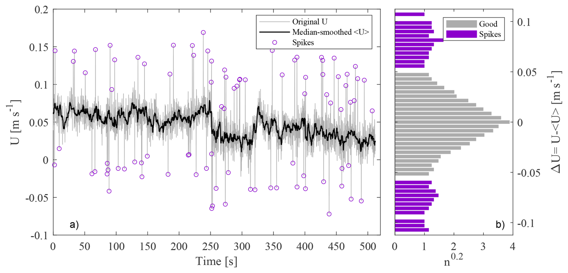
Figure 4Example of the despiking procedure adapted from Brock (1986). (a) Original velocities and smoothed signal obtained by applying a median filter over 2fs+1 samples. (b) Histogram of the difference between the original and smoothed velocity timeseries during the first despiking iteration. A power of 0.2 was applied to the number of samples n in each histogram bin for clearer visible confirmation of the spike thresholds. The ΔU=0 threshold for identifying spikes was determined from this histogram as the first instance where n=0 above and below ΔU=0. In this example, the thresholds for accepting velocities as good is −0.056 m s−1 < ΔU < 0.051 m s−1. If no bins have n=0, then the ΔU corresponding to the minimum n is used for setting despiking thresholds.
4.1.4 Formation of data quality flags
Each step flags velocity samples that do not meet the quality-control criteria. Each criterion uses binary (1/0) values that are then transformed into a “bitwise” flag. The maximum flag value depends on the number of criteria Nc used to assess data quality. The overall value of the boolean flag increases as the number of failed quality-control metrics increases. The maximum possible value for the flag will be less than , which translates to 255 when eight quality-control metrics are being evaluated (Nc=8).
To flag the raw velocities, we use an 8 bit boolean number calculated from:
where j is the flag number amongst those applicable to each velocity sample. For example, if the second and fifth quality-control flags apply to the velocity samples, translating to a boolean value of 18. These boolean flags allow tracking the state of multiple metrics simultaneously while reporting only one number. A value of 0 means the velocity sample was not flagged and thus is likely high-quality. These boolean flags were designed with the Climate and Forecast (CF) metadata conventions (https://cfconventions.org/cf-conventions/cf-conventions.html#flags, last access: 11 March 2026) in mind.
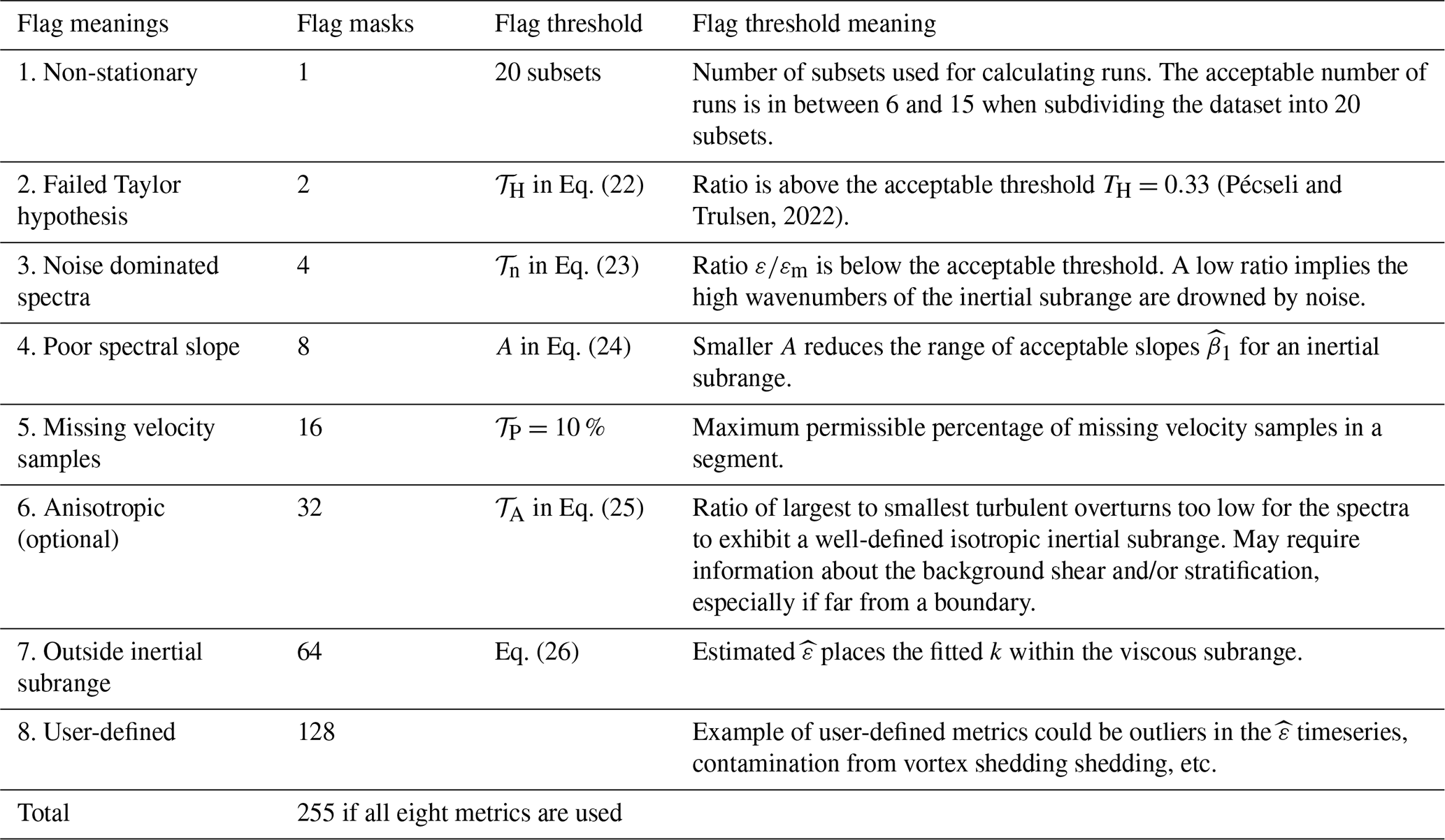
Flags are identifiable in the NetCDF file by the FLAG suffix appended to the variable name, i.e., XYZ_VEL_FLAG for raw velocities collected in the instrument's XYZ coordinates, or EPSI_FLAG for estimates (Tables A1 and A4 in Appendix A). We also included additional metadata in the variables' attributes. We added “flag thresholds” and “flag thresholds meanings” to CF recommended “flag_meanings” and “flag_masks” attributes (see Table 2). The “flag thresholds” provide the thresholds associated with a given flag, while the “flag thresholds meanings” briefly explain how the thresholds are applied. These extra attributes allow future users to revisit the flags, particularly the thresholds used, and apply more stringent (or less stringent) thresholds at their discretion. We also recommend that the these quality-control flags be briefly described in the methods of publication, along with the chosen thresholds for each flag.
(Brock, 1986)Table 2Summary of the different boolean flags and thresholds used to flag raw velocity samples. This information is stored with the suffix _FLAGS appended to the velocity variable name at the first processing level (Table A1). None of the MAVS datasets were flagged at level 1. As contamination from vortex shedding impacts the quality of estimates, these data are flagged at level 4.
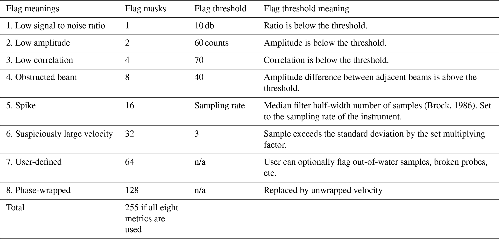
n/a – not applicable.
4.2 Segmented timeseries
At Level 1, quality control of the raw velocity measurements was completed. For the spectral calculations required to compute ε, (1) the measurements must be segmented in time, (2) flagged data must be replaced, (3) the velocities must be rotated into the frame of reference of the mean flow, and (4) the rotated velocities must be detrended to calculate the velocity fluctuations in the mean, transverse, and vertical directions.
The time series must be segmented before computing properties of turbulence. Selecting the length of the segments requires a balance between using sufficient data to resolve the inertial subrange in wavenumber space, while still ensuring stationarity of the turbulence. Stationarity implies that the key properties of the flow do not change over timescales shorter than the length of the segment. For many aquatic systems, this time scale is on the order of 5–15 min. If burst sampling is used because continuous sampling is unfeasible for the duration of the deployment, the segmenting considerations discussed below should be incorporated into the experimental design, as each burst is typically considered a segment. However, it is possible to break up bursts into segments if they are long enough (e.g., Tidal slough ADV benchmark in Table 1). These choices are made at the data processing stage for continuous time series.
The choice of segment length τε for estimating the dissipation impacts the resolvable wavenumbers of the inertial subrange and ultimately the statistical accuracy of the final spectrum to be computed. As described below (Sect. 4.3), a fast Fourier transform (FFT) is used to convert the time series into frequency space. The number of velocity samples NFFT included in each FFT, the sampling frequency fs, and the mean velocity dictate the spectral resolution and the smallest resolvable wavenumbers :
The duration of each FFT-length is given by . The low wavenumber and resolution that resolves theoretically at least one decade of the inertial subrange is given by:
When a decade is resolved, ten spectral samples Ns are available for spectral fitting (Fig. 5b). This wavenumber resolution depends on the ε (Fig. 5a), while the FFT duration τFFT depends also on the mean speed past the sensor (Fig. 5c). Increasing the τFFT by a factor of 10 allows for 100 spectral samples to be theoretically resolved in the inertial subrange (Fig. 5b). Once a τFFT is chosen, the total duration of each segment (or burst duration) for estimating dissipation τε≥2τFFT, and preferably τε≥3τFFT. These choices ensure the spectra have sufficient statistical certainty (degrees of freedom) for fitting (Bluteau, 2025a).
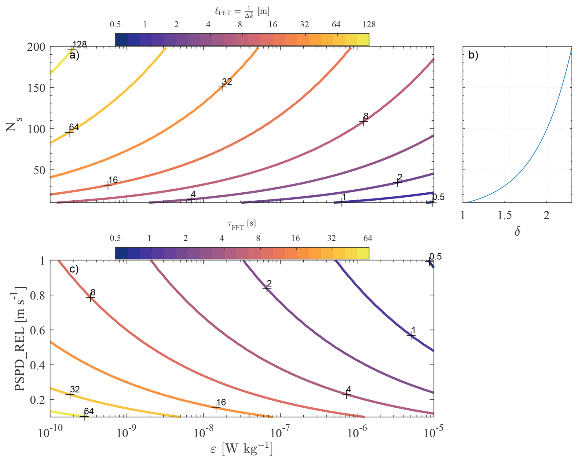
Figure 5(a) Minimum FFT length scale ℓFFT that must be resolved by the spectra as a function of ε and the number of fitted spectral samples Ns. The lowest resolved wavenumber and resolution . (b) The number of spectral samples available for fitting as a function of the number of resolved decades within the inertial subrange. (c) Minimum FFT-length duration τFFT required for resolving Ns=10 spectral samples within the inertial subrange. Note (a) and (c) represent minimum lengths and durations since the available bandwidth for spectral fitting may be reduced because of measurement noise and/or anisotropy.
With real observations, we recommend first selecting τFFT from Fig. 5c using the lowest expected ε and a relatively low derived from the observations. The spectra can then be estimated and plotted in wavenumber space against the theoretical velocity spectra in a similar format as Fig. 2. This visual representation can immediately show whether the chosen τFFT is longer than necessary (e.g., Tidal Shelf High Quality example in Fig. 2) or if the length needs to be extended because the high wavenumbers are drowned by noise. The goal is to choose a τFFT that is sufficiently long to resolve a decade of the inertial subrange throughout the entire dataset. The duration τFFT will be longer than necessary when ε or increases (Fig. 5c). For our benchmarks, the total segment duration varied from 82 s for the high-energy Tidal MAVS benchmark to 1024 s for the low-energy Under-ice MAVS benchmark (Table 1).
The Level 1 flags can exclude data points from further analysis. Once the time series has been segmented, data loss due to flagged points must be addressed before spectral calculations. For spectral computations, these excluded data points must be replaced in the time series as appropriate. There are several strategies for replacing missing data, including linear interpolation, using the variance of the signal (a technique commonly used in eddy covariance studies, e.g. Davis and Monismith, 2011), or using an unevenly spaced least-square Fourier transform (i.e., no replacement at all). These replacement strategies were trialed with one of the cleanest benchmarks (Underice MAVS sampling at 8 Hz) with randomly removed data in varying length gaps. For all tests, linear interpolation did the best job in recovering the original spectra, followed by the unevenly spaced techniques. From these tests, it is recommended that linear interpolation replace missing points and record the percent of good samples in each segment in the NetCDF Level 2 and 4 data. Segments with more than 10 % missing data should be flagged and rejected (Table 3). The threshold chosen for rejection should be recorded at Level 4 in the NetCDF file within the EPSI_FLAGS metadata (Table A4).
To estimate ε from all the different velocity components, the measurements must be rotated into the main direction of the flow. In some instances, the instrument's frame of reference may be aligned with the direction of flow, which is ideal to account for the varying levels of anisotropy among components (Gargett et al., 1984; Bluteau et al., 2011). If this alignment isn't set, then the velocities' measurement frame must be rotated into that of the flow, which we refer to as the analysis frame of reference. This process can be done by using the time-averaged velocities in each segment. If only the vertical velocity component will be used for calculation ε, then this step may not be necessary. The frame of reference for velocity analysis is noted in the NetCDF metadata within the Level 2 hierarchal group (Table A2). These velocities should be stored at Level 2 in a 3-D matrix UVW_VEL with dimensions [N_SEGMENT, N_SAMPLE, N_VEL_COMPONENT] with the rotation method (if any) for obtaining UVW_VEL velocities noted in the Level 2 metadata. Each N_SEGMENT are associated with a unique timestamp taken at the mid-point of each segment and stored in the TIME variable. We also store at Level 2 the variables ROT_AXIS and ROT_ANGLE, which can be used for rotating velocities from the measured coordinate system (e.g., XYZ_VEL) into the analysis frame of reference UVW_VEL (Table A2). This information is helpful for recovering the velocities of each segment in the original frame of reference.
4.3 Spectral observations
The parameters chosen when computing spectra can restrict the range of resolved wavenumbers, thus impacting the suitability of the spectra for estimating dissipation rates . In particular, spectra must resolve as much of the available inertial subrange as possible (Fig. 2) while considering how measurement noise may dominate the high wavenumbers close to the viscous subrange, which tend to be more isotropic than low wavenumbers. These choices also impact the statistical reliability of the velocity spectrum, and thus obtained from fitting algorithms as well as the accuracy of the spectral slope estimates (Bluteau, 2025a) – a quality-control indicator presented below in Sect. 4.6.
Our recommended spectral averaging involves splitting the time series into Nf subsets that are 50 % overlapped and windowed using a Hanning function (see Sect. 3.3 of ATOMIX paper on shear probes for review of spectral averaging; Lueck et al., 2024). An FFT is applied to each windowed subset before computing the squared magnitude to get the power spectral density estimates (Chap. 8 for pwelch methods; Percival and Walden, 2020). These power spectral density of all subsets are then averaged together to yield the spectra used for estimating ε. When computing spectra from 50 % windowed time series with a Hanning (cosine) window results in degrees of freedom d:
with c=1.9 (Eq. 416 of Percival and Walden, 2020) or c=1.92 according to Nuttall and Carter (1980). With our suggested segment duration of τε≥3τFFT (Sect. 4.2), Nf≥5 since . The resulting spectral observations will have about 10 degrees of freedom, i.e., d≈10. This recommendation is based on log-based fitting methods returning within a factor of about 1.5 of the actual value when applied to synthetic spectra with d=10 (Bluteau, 2025a).
4.4 Estimates of turbulent kinetic energy dissipation ε
We now discuss obtaining ε from the spectral observations, which involves spectral fitting Eq. (2) to the wavenumbers within the inertial subrange. We will focus first on the fitting methods before addressing how to identify the wavenumbers that belong to the inertial subrange, as these wavenumbers depend on ε – the sought quantity.
4.4.1 Spectral fitting techniques
We considered six methods to fit the model Ψj(k) to the spectral observations Φj(k), and subsequently estimate ε. Four methods fit the model spectra directly to the spectral observations, while the two remaining methods fitted log-transformed spectral observations by minimizing the sum of squared residuals or minimizing the sums of the absolute residuals (logLSQ and logLAD methods in Bluteau, 2025a). Of the four methods applied directly against the spectral observations, two methods minimized the sum of squared residuals using a gradient or gradient-free minimization algorithms (power and LSQ methods in Bluteau, 2025a). The third method in this category minimized the absolute residuals using the same gradient-free minimization as the LSQ method (LAD method in Bluteau, 2025a). The fourth method tested relied on the maximum likelihood estimator and presumed statistical distribution of the spectra (MLE method in Bluteau, 2025a). The full details of the methods and their assessment against synthetic spectra are described in Bluteau (2025a). Spectra were synthesized by specifying ε in Eq. (2) and adding uncertainty to the spectra via two different statistical distributions (Bluteau, 2025b). The sensitivity of the fitting methods was also evaluated against the uncertainty (smoothness) of the spectral observations, the number of spectral samples Ns, and the decadal range:
between the first k1 and the last kN fitted wavenumber (Bluteau, 2025a).
From that analysis, we recommend using fitting methods applied to log-transformed spectral observations. These methods returned more accurate results than those applied to untransformed spectra (Figs. 3 and 4 of Bluteau, 2025a). These methods were less sensitive to outliers that might be introduced in the spectra by unremoved spikes in the raw timeseries. Specifically, we recommend minimizing the least-absolute deviation (residuals) between the fitted model and the observations (logLAD method in Bluteau, 2025a). This method requires no assumption about the statistical distribution of the observations, unlike least-square regression, which expects normally distributed data. Minimizing the absolute residuals is considered less mathematically stable than least-square regression (Tercan, 2021). However, since only the intercept β0 that best fits the log-transformed spectral observations is required; the technique amounts to:
The spectral slope β1 is set to the expected value of for the inertial subrange (Eq. 2), and i denotes each observation in the spectra. Linear least squares would take the mean of Eq. (13) rather than the median. Both least-square regression and least-absolute deviation performed well against the synthetic spectra (Bluteau, 2025a). However, the estimated from least-absolute deviation were less biased than other methods, especially for spectra with low degrees of freedom, i.e., high degrees of uncertainty because of limited spectral averaging from using short segments τε.
From the fitted intercept , we can estimate using:
where ajCk are the constants already defined above for the inertial subrange model (Eq. 2). Using the logLAD fitting method and FFT-lengths that are of the segment length (d≈14), the estimated is expected to be within 43 % of the actual ε if ten samples are fitted over one decade (Figs. 3 and 4 of Bluteau, 2025a). This error reduces to 15 % when the number of samples increases to 100, which tends to occur when the fit falls at wavenumbers nearing the high wavenumber limit of the inertial subrange.
The synthetic spectra were also used to evaluate the ability of the fitting technique to estimate the spectral slope (Bluteau, 2025a). The spectral slope estimates help flag spectra that do not exhibit a clear inertial subrange because of poor data quality, low energy, and anisotropy, or simply because the sampling protocol or spectral averaging cannot resolve the inertial subrange. The latter occurs when sampling too slowly or using fft-lengths that are too short to resolve the entire inertial subrange (Sect. 4.3). As with the estimation of , the methods applied to the log-transformed data were better at recovering the spectral slope than those used to untransformed data. The logLAD method was less sensitive to outliers than the least-square regression (Bluteau, 2025a). The logLAD method involves minimizing the sums of absolute residuals rather than the sums of squared residuals (see Eqs. 7 and 4, respectively of Bluteau, 2025a).
4.4.2 Locating the inertial subrange in spectral observations
A primary challenge in obtaining is identifying the spectral wavenumbers that most likely belong to the inertial subrange, as these wavenumbers depend on – the sought quantity. Additionally, the location in wavenumber space also depends on the mean speed past the sensor when converting timeseries into spatial spectra. With appropriate choices for data sampling, segmenting (Sect. 4.2), and spectral averaging (Sect. 4.3), this step amounts to avoiding the low wavenumbers dominated by anisotropy and the high wavenumbers dominated by instrument noise. Other wavenumbers to avoid are those impacted by vortex shedding off instrument frames (e.g., Under-ice MAVS in Fig. 2), or surface waves.
We evaluated four strategies for identifying the inertial subrange within the spectra by adding white noise to the same synthetic spectra used to test fitting methods (Bluteau, 2025a, b). The two first strategies require computing the absolute deviation between each of the fitted log-transformed spectral observations and its log-transformed model spectrum given by Eq. (2):
and then taking the mean or median of these deviations across different subsets of wavenumbers (Fig. 6d, e respectively). The third strategy estimated the mean absolute deviation of (Eq. 24 of Ruddick et al., 2000). Our fourth strategy estimated and the spectral slopes over short wavenumber subsets of the spectra (see Fig. 6c). The wavenumbers with the estimated slope closest to the expected for the inertial subrange are then selected to calculate the spectrum's final . The other three methods situate the inertial subrange over the wavenumbers that yield the minimum value for the calculated statistics.
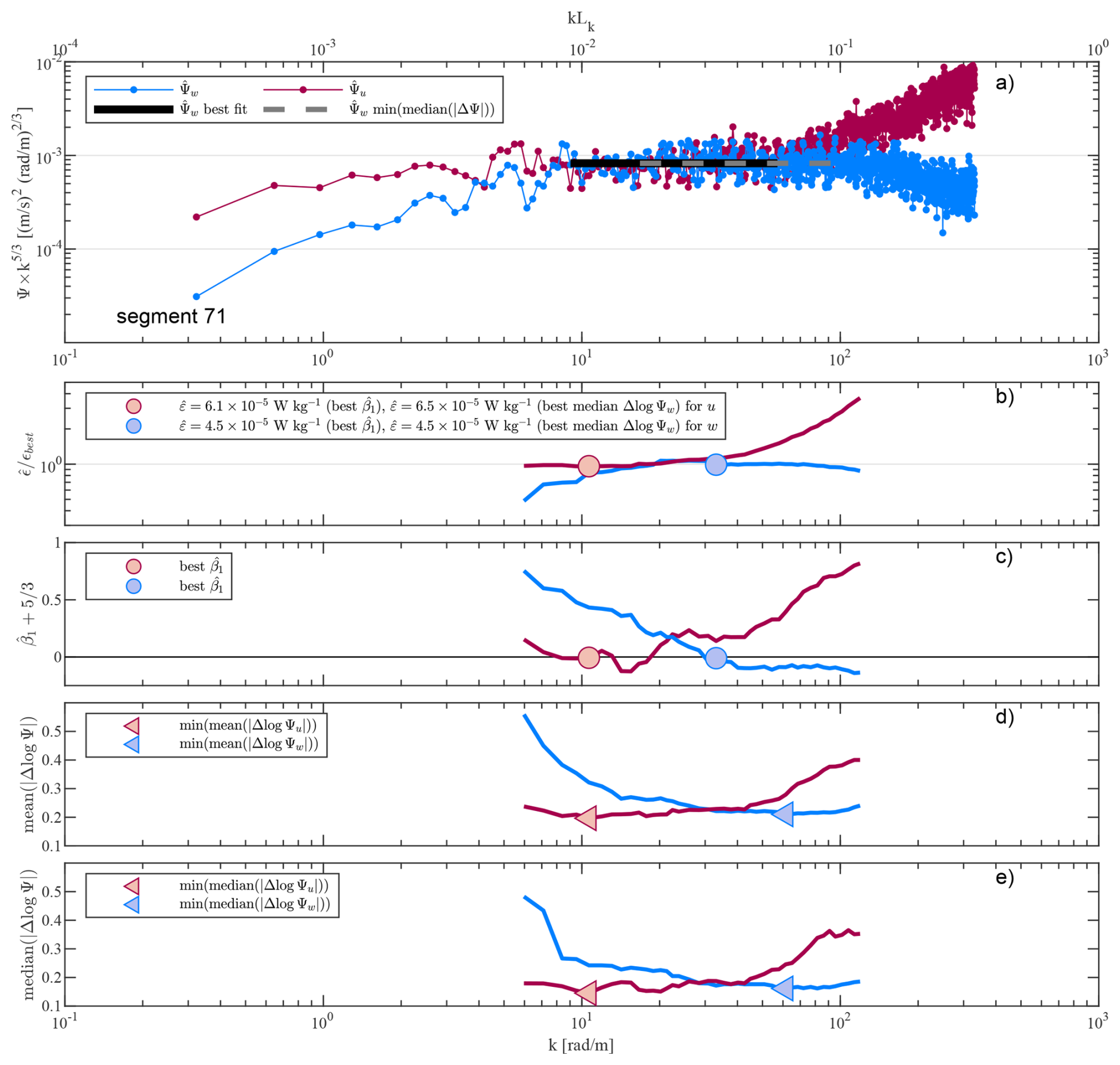
Figure 6Example of locating the inertial subrange from (a) the spectra of two velocity components collected concurrently in the Tidal Shelf ADV. (b) Deviation of the estimated from each subset that included a decade's worth of spectral samples. εbest is the that yields the spectral slope closest to the expected presented in (c) in the vertical velocity direction. The top secondary x-axis in (a) shows the non-dimensional wavenumber based on the εbest estimated from the vertical component that was less impacted by measurement noise. (d) Mean of the absolute deviation between the log-transformed spectral observations and the fitted value over each subset (Eq. 15). (e) Same as (d) but taking the median instead of the mean. The triangles in both (d) and (e) represents the median wavenumber where the most likely wavenumbers representing the inertial subrange would be identified from these two methods.
The slope method was recommended because it performed slightly better than the other three against synthetic spectra of Bluteau (2025b) for which we added white noise floor to mimic the impact of instrument noise on observed spectra. The slope method tended to situate the inertial subrange at lower wavenumbers than the other three methods even when the synthetic spectra were further flattened by adding white noise at low wavenumbers. This additional flattening crudely replicated the narrowing of the inertial subrange when the energy containing range begins to impinge on the inertial subrange (e.g., cpm for Tidal Shelf ADV example in Fig. 2). We note, however, that all four methods generally situated the wavenumbers within the inertial subrange of the synthetic and real spectra (e.g., Fig. 6c–e). Overall, we recommended the slope method because it performs slightly better than the other methods, while the estimated slope β1 is required later for flagging of at level 4.
In practice, the user must select the size of each subset, in addition to the wavenumber overlap for each subset within the spectra. For our benchmark datasets, we used an overlap equivalent to of a decade, but other users may prefer shifting the window by one spectral sample at a time. We recommend a minimum decadal wavenumber range of δ=0.8 and that each fitted subset includes at least ten samples, especially when δ<1 (Bluteau, 2025a). Users may also specify a maximum kmax and minimum wavenumbers kmin that can be fitted upon inspection of the spectral observations (e.g., Fig. 2). For example, where Lb is the distance to the nearest boundary, while depends on the dimension ℓ of the sampling volume of the instrument. For each subset, the estimated is used to calculate LK, and verify whether the fitted wavenumbers are within the inertial subrange. The user may provide some allowance, but we recommend ensuring that the median fitted kmed is within the inertial subrange, i.e., . Spectra for which none of the fitted subsets satisfy this requirement were flagged (see Sect. 4.6).
4.4.3 Impact of noise on ε estimates
In some instances measurement noise may adversely impact the estimated , and render the spectra unusable for estimating turbulence quantities. The drowning of the inertial subrange by noise is particularly common in low-energy environments such as the ocean interior or in lakes. To deal with this issue, some authors have presumed the shape of the noise spectra to either remove it from the spectral observations (e.g., Davis and Monismith, 2011), or add the presumed noise shape to the model used for fitting the unaltered spectral observations (e.g., Ruddick et al., 2000). The former is challenging because measurement noise levels change with the flow conditions and must be estimated from the spectra itself (see Voulgaris and Trowbridge, 1998). The noise floor can be particularly hard to estimate in high energy flows being drowned by the signal. The latter method has the same challenges but prevents us from using spectral fitting methods applicable to log-transformed spectra. Rather than use these strategies, we recommend comparing the estimated to the minimum εm when the corresponding theoretical spectral energy levels in the inertial subrange (Eq. 2) exceeds the noise floor Φn (Bluteau et al., 2011):
This recommendation is based on the relatively low positive bias introduced when leaving the noise “as-is” in the spectra (Fig. 7). The noise floor Φn typically appears as white noise (flat) in velocity spectra and can be estimated by averaging the energy levels of the highest wavenumbers where . Equation (16) depends on the fitted wavenumbers k and can be generalized further as a function of the smallest turbulent length scales LK defined in Eq. (3) (Bluteau et al., 2011):
The inertial subrange corresponds to α≤0.1. Substituting this relationship for k into Eq. (16) yields the following minimum εm:
This equation demonstrates that noise is most detrimental when fitting wavenumbers approaching the theoretical high wavenumber bound of the inertial subrange (). The minimum resolvable εm can be viewed as the measurement detection limit. The limit increases with noise levels, albeit the increase is amplified when when fitting large wavenumbers i.e., k close to the beginning of the viscous subrange (Fig. 7). For example, the inertial subrange sits above the noise floor for W kg−1 at wavenumbers ten times smaller than the highest within the inertial subrange (α=0.01) provided the noise levels Φn are less than 10−6 m2 s−2 (rad m−1)−1 (Fig. 7a). However, if fitting the highest wavenumbers within the inertial subrange (α=0.1), the spectra sit above the noise floor only if m2 s−2 (rad m−1)−1 (Fig. 7b).
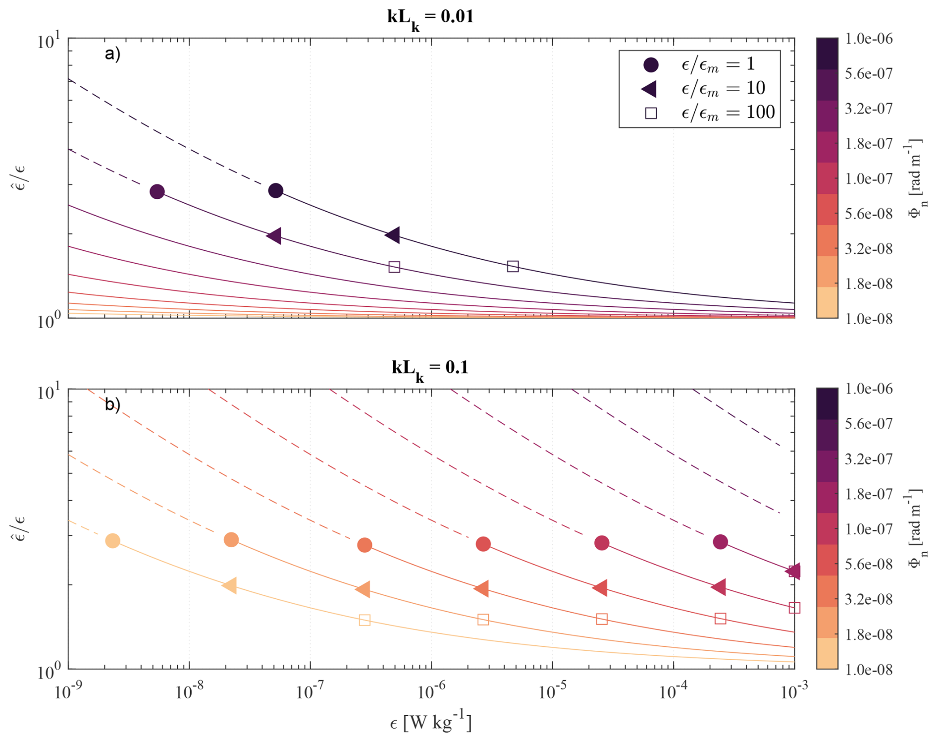
Figure 7Over-estimation of as a function of noise level Φn and wavenumber fitted. The fitted wavenumber in (a) corresponds to α=0.01; in (b), to α=0.1, the high wavenumber k limit for the inertial subrange. The circles show the minimum resolvable dissipation εm (Eq. 18). The dashed line indicates that the inertial subrange sits below the noise floor; thus, cannot be resolved. LK is the Kolmogorov length scale that defines the smalles turbulent scales (Eq. 3).
By leaving the noise floor “as-is” in the spectral observations, a positive bias occurs when estimating . The over-estimation is in addition to other errors associated with spectral fitting techniques described above. When , the estimated over-predicts the prescribed value ε by a factor of 3 (circles in Fig. 7). When , the estimated over-predicts ε by a factor of 1.5 (squares in Fig. 7). These positive biases are relatively small compared to the range of ε encountered in environmental flows, especially considering how quickly the bias lessens when including lower wavenumbers (α≤0.1) in the fit. Hence, the biases shown in Fig. 7 are conservative when α is determined from the largest fitted wavenumber kN.
To flag overly noisy spectra with Eq. (18), the user must estimate the spectral noise floor Φn from the observations. For our benchmarks, Φn was calculated as the average spectral energy levels over the last δ=0.1 decadal range or the last 30 spectral samples, whichever leads to a larger number of averaged samples. The resulting Φn is stored as SPEC_NOISE_UVW in the same units as the spectra from which the average was determined at Level 3 UVW_VEL_SPEC. The spectral noise estimate Φn is used with the maximum fitted wavenumber kN stored in K_BNDS and the estimated dissipation stored in Level 4 to estimate εm using Eq. (18). The estimated εm is stored as MIN_EPSI_NOISE at Level 4 so that this value can be used to generate quality control flags for in Sect. 4.6.
4.4.4 Flow interference
Nearby instrument frames may obstruct the flow or shed vortexes, contaminating the velocity observations. This contamination is often recognizable as a narrow band peak in the velocity spectra when the frame obstruct the flow upstream of the sampling following (Fig. 2). In this situation, the contamination frequency fc can be determined from the Strouhal number Sr:
for high Reynolds flow (Sr≈0.21, Kundu, 1990). The frequency of the disturbances increases with decreasing diameter D of the obstruction or an increase in the velocities past the frame . These disturbances are typically associated with a specific flow direction relative to the instrument's frame of reference. Hence, if the instrument is fixed in space, the flow direction can be used to identify when vortex shedding is potentially contaminating the velocity spectra, Alternatively, near boundaries, the estimated can be compared to the predicted values for the log-law of the wall and the flow direction (see Fig. 4 of McGinnis et al., 2014). This contamination may occur at wavenumbers higher than those within the inertial subrange, as apparent in the first 25 min of the Tidal Shelf ADV benchmark. The flow disturbances will sometimes be significant enough to increase energy levels within the inertial subrange. Thus, it is preferable to avoid the problem by placing the sampling volume of the instruments far from the obstruction. A common rule of thumb is leaving a space larger than ten times the diameter of the obstruction between the frame and the sampling volume. When the sampling volume is obstructed, will be over-estimated downstream of the disturbance (see Fig. 4 of McGinnis et al., 2014).
Another contamination source specific to the MAVS velocity sensor is the rings that house the acoustic transducers. These rings shed vortexes, contaminating the velocity measurements. This contamination affects most directions transverse to the instrument's main shaft. For a horizontally mounted instrument, such as our Tidal MAVS benchmark, the longitudinal direction was the least affected by the rings' vortex shedding (Hay et al., 2013). In contrast, the transverse direction was the most affected. The other Under-ice MAVS benchmark was mounted vertically on a rod lowered beneath the ice. The vertical velocity direction was the least affected, followed by the longitudinal, although the vertical component still shows evidence of a high-frequency flow disturbance in its spectra (Fig. 2). Our quality-control metrics below include optional flagging for estimates affected by flow disturbances.
4.5 Confidence intervals for
Given the above recommendation for fitting the spectra using the least-absolute deviation method, we suggest creating confidence intervals on using bootstrapping techniques (Davison and Hinkley, 1997). The advantage of bootstrapping is that no assumption is made about the statistical distribution of the observations. Bootstrapping involves resampling the dataset and recomputing the desired statistics to provide a distribution of estimates, from which confidence intervals can be obtained. For our application, we bootstrapped the fitted since it is used to estimate from Eq. (14). This step is achieved by resampling the residuals r between the log-transformed observations () and the best-fit :
and adding them to the best-fit line in log-log space to create a new dataset :
where i represents an observation and , the bootstrapped residuals. The new spectral log-transformed spectra are refitted with Eq. (13) to obtain a bootstrapped estimate. The resampling of residuals and fitting are repeated many, typically more than 1000, times (Davison and Hinkley, 1997), to obtain a collection of bootstrapped estimates for a given velocity spectrum, and thus estimate. Finding the 2.5th and 97.5th percentiles from the collection of provides the 95 % confidence interval. These percentiles are then substituted into Eq. (14) to obtain the confidence levels for . In the benchmark datasets, we obtained the 95 % confidence intervals for each estimate by resampling the residuals and refitting 1000 times (Eq. 21).
4.6 Quality-control considerations and flags
Similarly to the raw velocities at Level 1, we assess our estimates against multiple quality-control metrics. The results of this assessment are stored using an 8 bit (Nc=8) boolean flag calculated with the same equation as for our raw velocities (Eq. 8). Thus, the maximum flag value is 255 when all eight quality-control metrics apply to a given estimate. The use of boolean codes allows for flagging estimates for one or multiple reasons at once. This number is stored at Level 4 as EPSI_FLAGS. Below we describe each metric individually, which are summarized in Table 3.
(Pécseli and Trulsen, 2022)Table 3Summary of the different boolean flags and thresholds used to mask ε estimates, stored as EPSI_FLAGS variable in the 4th processing level within NetCDF file.
4.6.1 Non-stationarity
Our first metric presents the results from testing the stationarity of turbulent velocities. Both spectra computations and the inertial subrange model rely on the assumption of stationarity. The test is applied to each velocity component separately. For this purpose, we used the nonparametric test by Bendat and Piersol (2000), which involves calculating two statistics (standard deviations and average) over shorter subsets of each velocity timeseries segment (of duration τε). We then compare the number of runs (crossings) of each statistic about its average to the expected values in Table A.6 of Bendat and Piersol (2000). For this evaluation, the user must choose the significance level and the number of subsets to subdivide each segment. We used 20 subsets and a 95 % level, resulting in an acceptable number of runs between 6 and 15. We flagged as non-stationary if the number of runs for the standard deviation and means for the velocity segment are outside the expected range.
4.6.2 Violation of Taylor's frozen hypothesis
The second quality metric focuses on Taylor's frozen turbulence hypothesis. We recommend flagging estimates associated with low advection velocities relative to the root mean square of the turbulent velocity fluctuations along the direction of mean advection urms. This condition translates to flagging associated with exceeding a threshold 𝒯H:
We suggest 𝒯H=0.33 based on the work of Pécseli and Trulsen (2022) who showed that the error for for this value is about 10 %. Larger errors are expected when increases (see Fig. 12 of Pécseli and Trulsen, 2022). Thus, 𝒯H could be increased but it should always remain smaller than 1. The chosen threshold should be specified in the metadata of EPSI_FLAGS accompanying the estimates as detailed in Table 3.
4.6.3 Noise-dominated spectra
The third flag considers whether the fitted spectra are drowned by noise. This criteria involves calculating the minimum resolvable εm using Eqs. (17) and (18) from the dissipation estimates, the maximum fitted wavenumber kmax, and the estimate of the spectral noise floor Φn (see Sect. 4.4.3). The estimated is compared to the minimum resolvable εm. Dissipation estimates are flagged as being drowned by noise when the ratio between these two quantities is less than the user-defined threshold 𝒯n:
The threshold 𝒯n must always be larger than one and specified in the flag's metadata (see Table 3). We suggest 𝒯n=3 owing to the positive bias shown when the highest wavenumbers of the inertial subrange sit near spectral observations as illustrated in Fig. 7).
4.6.4 Spectral slope outside expected range
Our fourth flag involves estimating the spectral slope from the observations to identify spectral slopes that deviate too much from the expected value (thus rendering suspect the associated estimate of ). These deviations may occur because of excessive noise, anisotropy, or other contamination (e.g., vortex shedding). An estimated slope that deviates from can also occur when the slope is actually due to statistical variability of the computed spectra d, the number of spectral points Ns used for the fitting, and the decadal range δ fitted (Figs. 7 and 8 of Bluteau, 2025a). Their results were obtained by fitting the inertial subrange to 3200 synthetic spectra (100 spectra per degrees of freedom tested) with uncertainty generated using the -distribution (Bluteau, 2025b). Figure 8 recasts their results in a different form to show that the estimated 99.7 % bounds can be represented by:
with empirical estimates of A ranging between 7 to 17. The maximum A from the numerical experiments was about 17 for Ns=100 and δ=1 (Fig. 8). This A denotes the maximum deviation obtained from the expected when fitting idealized velocity spectra.
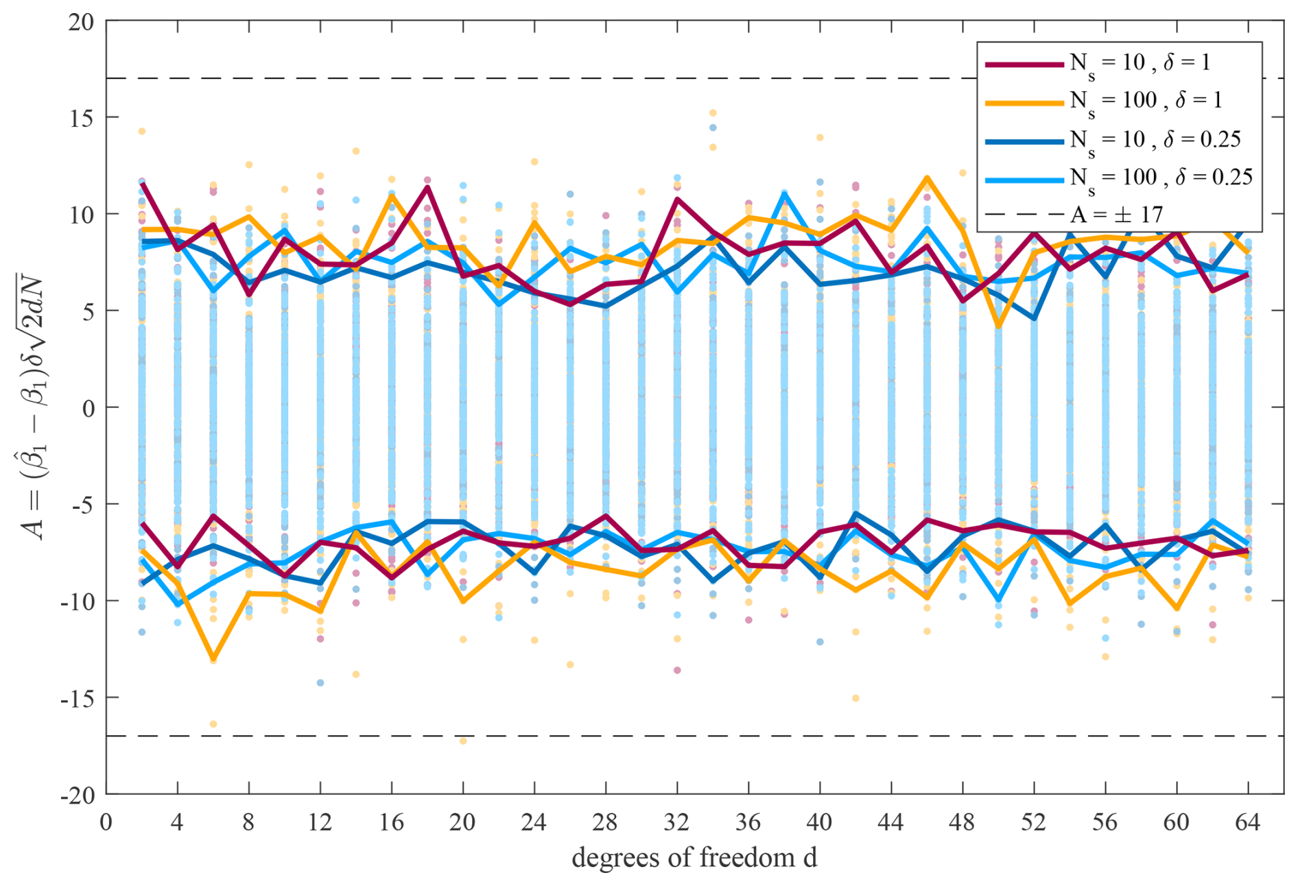
Figure 8Estimated A from computing spectral slopes using the logLAD method on the distributed synthetic spectra dataset Bluteau (2025a, b). The thick lines provide the 99.7 % bounds (0.15th and 99.85th percentiles) for the numerical experiments when changing the number of samples Ns and decadal range δ fitted. Results are scaled by the expected standard deviation of distributed samples () in addition to . This figure illustrates that deviation of from the true value scales approximately with . There were 3200 synthetic spectra fitted for each series of numerical experiments (100 spectra per degrees of freedom tested)
We chose this maximum A=17 to flag with spectral slope estimates that fall outside the bounds given by Eq. (24). Reducing A would render the threshold more stringent, flagging an increased number of estimates. Users should always specify their choice of A in the metadata of the Level 4 NetCDF quality-control flags (EPSI_FLAGS in Table A4). This information in combination with the variables for estimating the acceptable bounds (δ, Ns, and d in Eq. 24) should be also stored as variables at Level 4 to enable other users to re-flag if desired (see Table A5).
4.6.5 Missing too many samples
Our fifth flag involves identifying segments with significant data loss during the quality-control of raw velocities, which render the spectra unreliable for estimating (Sect. 4.1). Limited testing involving the random removal of velocity samples from our benchmarks showed that spectral shapes deviate considerably from the original when more than 10 % of samples are removed. As the percentage of data loss increases, the interpolated time series yield spectra with increased energy levels at low k and decreased energy at high k. We suspect acceptable data loss depends on data quality (i.e., noise levels) and underlying turbulence captured in the original time series. We thus recommend users specify their threshold 𝒯P for the maximum percentage of data loss in the segment after quality-controlling the raw velocities. For our benchmark datasets, we use 10 % as the minimum percentage of good samples in a segment.
4.6.6 Spectral anisotropy
The sixth metric is for flagging estimates associated with low energy turbulence, resulting in anisotropic spectra. This flag is not for excluding anisotropic spectra, when one velocity component is more impacted by the flow properties than the others. This impact manifests itself as flatter spectral slopes at low wavenumbers preferentially in one direction compared to the others (e.g., vs. for k<8 rad m−1, Fig. 6). This feature does not render the spectra unusable for estimating ε until the turbulence becomes so weak that the scales of the energy containing subrange start approaching those at the high end of the inertial subrange. The spectral slopes may start to deviate from the , but oftentimes a slope still exists but its energy levels drop below those expected for isotropic turbulence (Eq. 2). Spectra are considered too anisotropic when the ratio is small, which results in underestimating .
This flag is optional as it typically requires an estimate of the largest turbulent overturns L (see Sect. 2). The size of the large overturns depends on the mean flow characteristics and so necessitate measuring the background stratification (LO, Eq. 5) or the background shear (LS, Eq. 6) unless the distance from the boundary is a suitable alternative for L (Eq. 7). To flag this issue, we compare the ratio to a user-defined threshold 𝒯A:
The threshold 𝒯A depends on the chosen measure for L and the velocity component (see Bluteau et al., 2011, for an extensive review). The longitudinal direction tends to have a broader inertial subrange than the vertical and transverse directions. We recommend a similar threshold 𝒯A=100 to Bluteau et al. (2011), noting that higher thresholds might be necessary when the transverse or vertical components are used to estimate . The user should specify the definition of their largest L and the threshold 𝒯A for flagging the data in the EPSI_FLAG metadata. For our benchmarks, this length-scale was set L=κLb and stored as at level 4.
4.6.7 Fit located outside inertial subrange
The seventh flag identifies spectra when most fitted wavenumbers sit outside the inertial subrange. This situation arises when the median fitted wavenumber kmed during the search of the inertial subrange (see Sect. 4.4.2) are high and always lies within the viscous subrange:
(Pope, 2000). This situation typically arises when the speed past the sensor is very slow, or the spectra are very noisy, such that the algorithm places the inertial subrange at very high wavenumbers.
Alternatively, the fitted wavenumbers may be too small and thus outside the inertial subrange. This situation will arise if the inertial subrange is unresolved because the sampling frequency is too slow or the largest overturns' are negligible. For the benchmarks, these wavenumbers are those smaller than those dictated by the distance to the nearest boundary (see Fig. 2).
4.6.8 User-defined flags
The last flag is reserved for missing estimates or any other user-defined flag. For example, the user may flag data loss onboard the instrument, outliers in the time series, or perhaps unrealistically different between velocity components. Occasionally, all components will yield estimates, passing all quality control criteria, but significant differences still exist between components. This situation may occur, for instance, because of vortex shedding from nearby flow obstacles (Sect. 4.4.4). We used this user-defined flag to denote velocity directions from the MAVS benchmark datasets that were impacted by vortex shedding.
4.6.9 Final estimates
In the NetCDF file, a final estimate for is stored as a 1d timeseries EPSI_FINAL. This parameter is effectively the “best” issued from the data processing and flagging with the EPSI_FLAGS. There can often be large differences in dissipation estimates among the three velocity components caused by differing impacts of noise, anisotropy at low wavenumbers, and vortex shedding on the spectral observations. Thus, we select one of the velocity component to produce the final estimates, and document the choice in the EPSI_FINAL metadata.
We illustrate the methods, common data quality issues, and the application of quality-control flags for our Tidal Shelf ADV benchmark. The quality-control thresholds and processing choices are summarized in Table 4 for our four benchmarks. The velocities' “legged” appearance was caused by setting the velocity range below the maximum observed during deployment. This issue is rectified once beam velocities are unwrapped. These velocities were stored as XYZ_VEL_UNWRAP at level 1, and once quality-controlled, they are segmented and included in the NetCDF file at level 2 (Fig. 3 and Table A1). This dataset was high quality as the data return was more than 85 % for all segments (Fig. 9c). The most significant data loss coincided with the period of strong flows when many velocity samples were phase-wrapped. Despite the unwrapping, some poor velocity samples remained and were flagged using the 5 and 6th flags that denote spikes and suspiciously large velocities in Table 2. These samples appeared in the timeseries as having velocities flags totaling 160 and 176, respectively (Fig. 9c). For this dataset, the 8th flag, denoting phase-wrapped samples, was not used to discard velocity samples since these were unwrapped before segmenting. This flag yielded a boolean value of 128. Velocity samples were only discarded if flagged for any other reason. Only samples with flag values greater than 0 and not equal to 128 were replaced using linear interpolation at level 2 (see Sect. 4.3). This interpolated dataset was then split into 256 s long segments with a 25 % overlap between adjacent segments and stored in the Level 2 group within the NetCDF file.
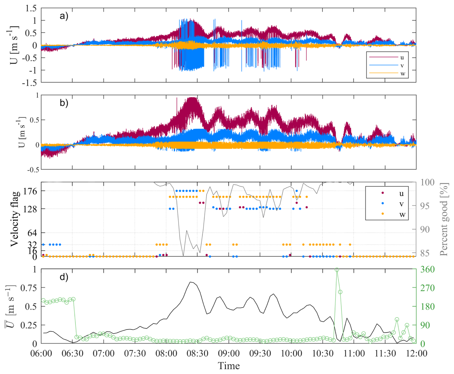
Figure 9Level 1 and 2 observations associated with the Tidal Shelf ADV benchmark. (a) Raw velocities with obvious signs of phase-wrapping. (b) Quality-controlled and unwrapped velocities for the benchmark. (c) Maximum boolean velocity flags (i.e., XYZ_VEL_FLAG) value for each 256 s long segment. The secondary axis shows the percentage of good samples within each segment. (d) Mean velocities and direction relative to the instrument's frame of reference. Table 2 summarizes the meaning of the velocity boolean flags.
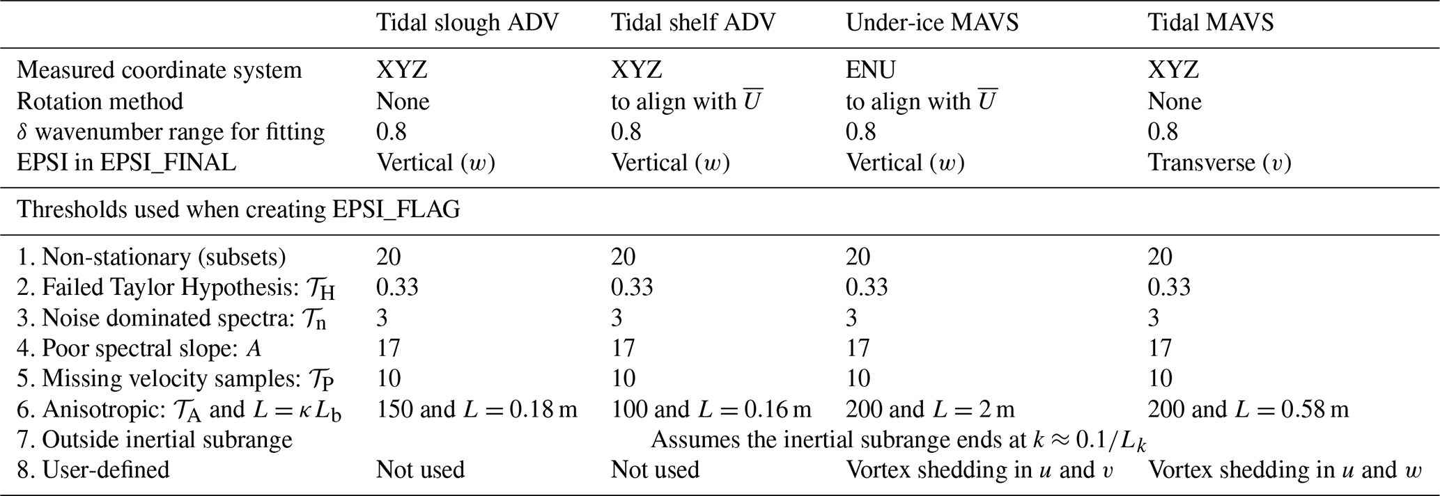
Table 4Data processing choices when estimating from quality-controlled velocities.
The Level 2 segmented and quality-controlled data were then used to calculate the spectra stored in the NetCDF file at Level 3. Spectra from four different segments of the Tidal Shelf ADV benchmark are illustrated in Fig. 10. This benchmark displayed evidence of vortex shedding when velocities were directed at 220° relative to the instrument's frame of reference and exceeded 5 cm s−1 (segments 1 to 7). However, the shedding was well outside the inertial subrange (100 cpm, Fig. 10a), so was not flagged for this criteria.
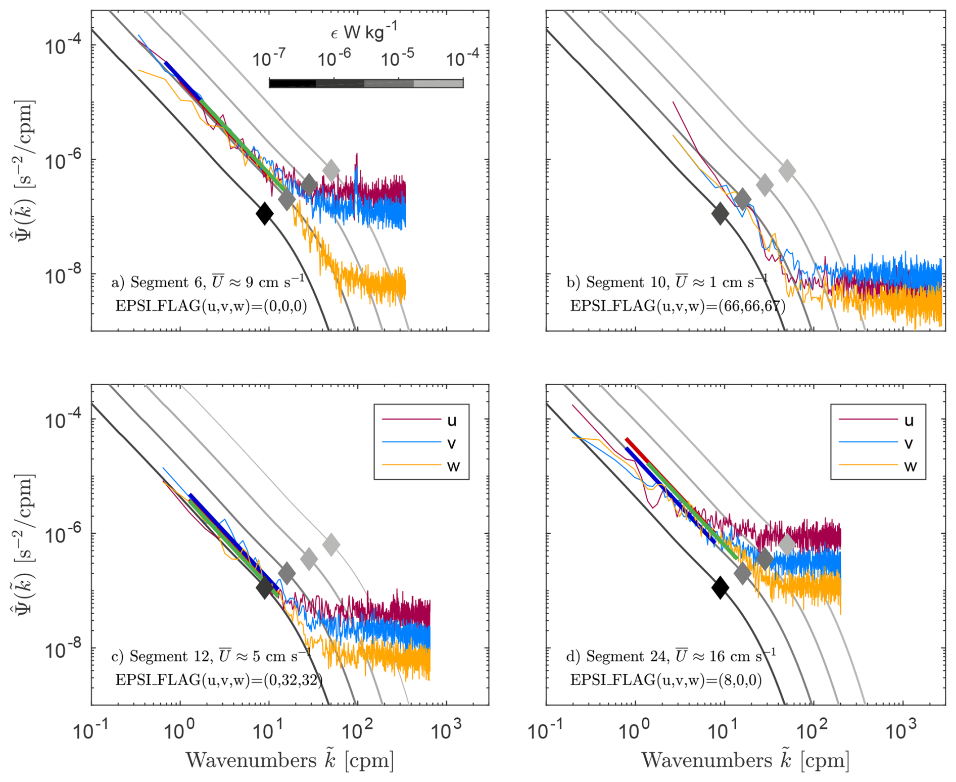
Figure 10Example spectra from four different segments of the Tidal Shelf ADV benchmark are shown in separate panels for all three velocity components. The turbulence model spectra for velocities are shown in gray for 10−7 (darkest) to 10−4 W kg−1 (lightest) as digitized by Luznik et al. (2007) from the work of Gargett et al. (1984). The approximate limit between the inertial and viscous subrange for each model spectra is denoted by the diamonds (Eq. 4).
The spectra from segments 8 through 10 were not impacted by vortex shedding because the flow was too weak despite the velocities being oriented in the right direction to contaminate the measurements (see segment 10 in Fig. 10b). In this second example, the estimates of all velocity components were nonetheless flagged for failing the Taylor Hypothesis criteria and for most of the spectra sitting within the theoretical viscous subrange based on the fitted (2nd and 7th flags, respectively, in Table 3). Combined, these two flags translate to a boolean value of 66 for the longitudinal and transverse flag stored at level 4 (Eq. 8). The vertical component had a larger flag of 67 because it was also deemed non-stationary (1st flag in Table 3).
For our third example, estimates from the transverse and vertical components received a boolean equal to 32 (Fig. 10c). This value translates to applying the 6th flag, concerning turbulence anisotropy (I∈6 in Eq. 8). For this dataset, we used a threshold of 𝒯A=100 to identify segments that were too anisotropic to yield a reliable estimate (Eq. 25, Table 4). The longitudinal component passed the condition for being sufficiently isotropic, while passing all other quality-control criteria (EPSI_FLAG = 0).
Our fourth and final example received an EPSI_FLAG of 8 in the longitudinal velocity component (Fig. 10d). This boolean code implies that this segment failed the 4th criterion, which indicates that the spectral slope (Fig. 11e) was outside the expected range based on Eq. (24). For this computation, we used d=28.5 for the spectra's degrees of freedom, N=32 for the number of fitted samples, and δ=0.8 for the decadal range fitted. The other two velocity components passed all quality-control criteria (EPSI_FLAG = 0).
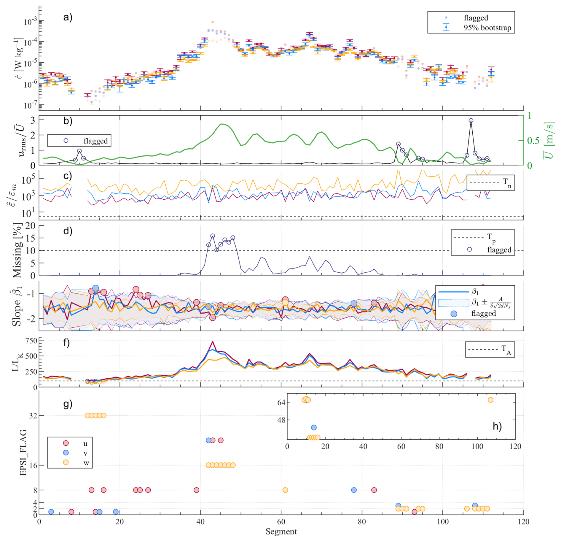
Figure 11Estimated and associated quality control metric used for flagging the Tidal Shelf ADV benchmark dataset. (a) The 95 % bootstrap confidence intervals are shown for the estimates that passed all quality-control metrics. If no error bars are presented, then the estimate was flagged for not meeting one or several quality-control criteria. (b) Taylor Frozen hypothesis (Eq. 22) with the mean speed past the sensor on the secondary right axis. (c) Noise-dominated spectra metric (Eq. 23). (d) Too many missing velocity samples compared to 𝒯P. (e) Spectral slopes β1 deviate from the expected range (Eq. 24). (f) Likely anisotropic spectra (Eq. 25). (g) Boolean flag for our estimated . The higher EPSI_FLAGS are show in (h).
Despite not flagging any of the from the Tidal Shelf ADV for vortex contamination, this contamination source did impact the reliability of of other benchmarks. For example, we flagged all of the MAVS estimates obtained from velocity components perpendicular to the instrument's shaft. This step translates to flagging all the Tidal MAVS estimates, which were not from the transverse (y) direction and all Under-ice MAVS estimates that were not from the vertical (w) direction (Table 4). The chosen velocity component for the final estimates differs between the datasets. The Tidal MAVS assigns the estimates from the transverse direction given the orientation of the flow relative to the instrument's shaft, while the other datasets assigned from the vertical component. Depending on the intended scientific purposes for the estimates, users may want to be more or less stringent when applying the quality-control metrics. Hence, we recommend documenting the chosen thresholds in the NetCDF metadata for EPSI_FLAGS.
This paper uses acoustic point-measurement data to describe a systematic approach to obtaining reliable estimates of a key ocean parameter – the dissipation rate of turbulent kinetic energy ε. We describe the processing and data handling steps, quality control, and associated flags. Finally, we provide benchmark results for researchers to validate their computer methodologies. For peer-reviewed publications, we recommend depositing in data centers, at a minimum, the Level 4 NetCDF group (see Tables A4 and A5). Providing example spectra like in Fig. 2, or alternatively providing the Level 3 NetCDF group (Table A3) is strongly encouraged. The publication's methods should summarize the data processing choices for quality-controlling the raw timeseries (Table 2) and for estimating from these velocities (e.g., Table 4).
This approach was developed as part of the ATOMIX working group. As such, parallel analyses exist for other ocean measurement measurement techniques (Lueck et al., 2024). There are benefits to this combined approach, including the ability to leverage a broader range of experience and coding and making the step from one type of measurement to another much easier. This benefit also applies to field campaigns with overlapping measurement approaches (e.g., the near-bed section of a shear profile overlapping with a region measured with a bed-mounted acoustic velocimeter).
One clear but simple conclusion is that there are significant benefits to consistently employing the ATOMIX naming and storage convention described here. In particular, this enables rapid integration with existing approaches and builds a more cohesive and efficient sampling community with enhanced cross-talk between researchers using different methods. Over time, we expect improvements to the best practices as new instruments become available and new environmental conditions are sampled. With the oceans' continued importance and role in key Earth system processes, more systematic sampling of the oceans is inevitable. It is important that this sampling produces results that are consistent and reliable.
Table A1Summary of Level 1 NetCDF data format. This level includes the full resolution raw timeseries velocities in physical units, quality-control flags, and ancillary data.
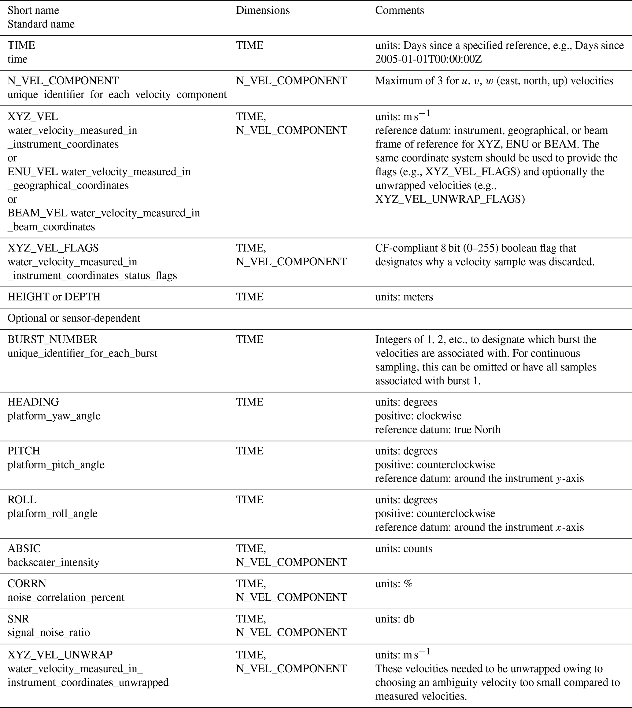
Table A2Summary of Level 2 NetCDF data format. This level includes quality-controlled and segmented timeseries.
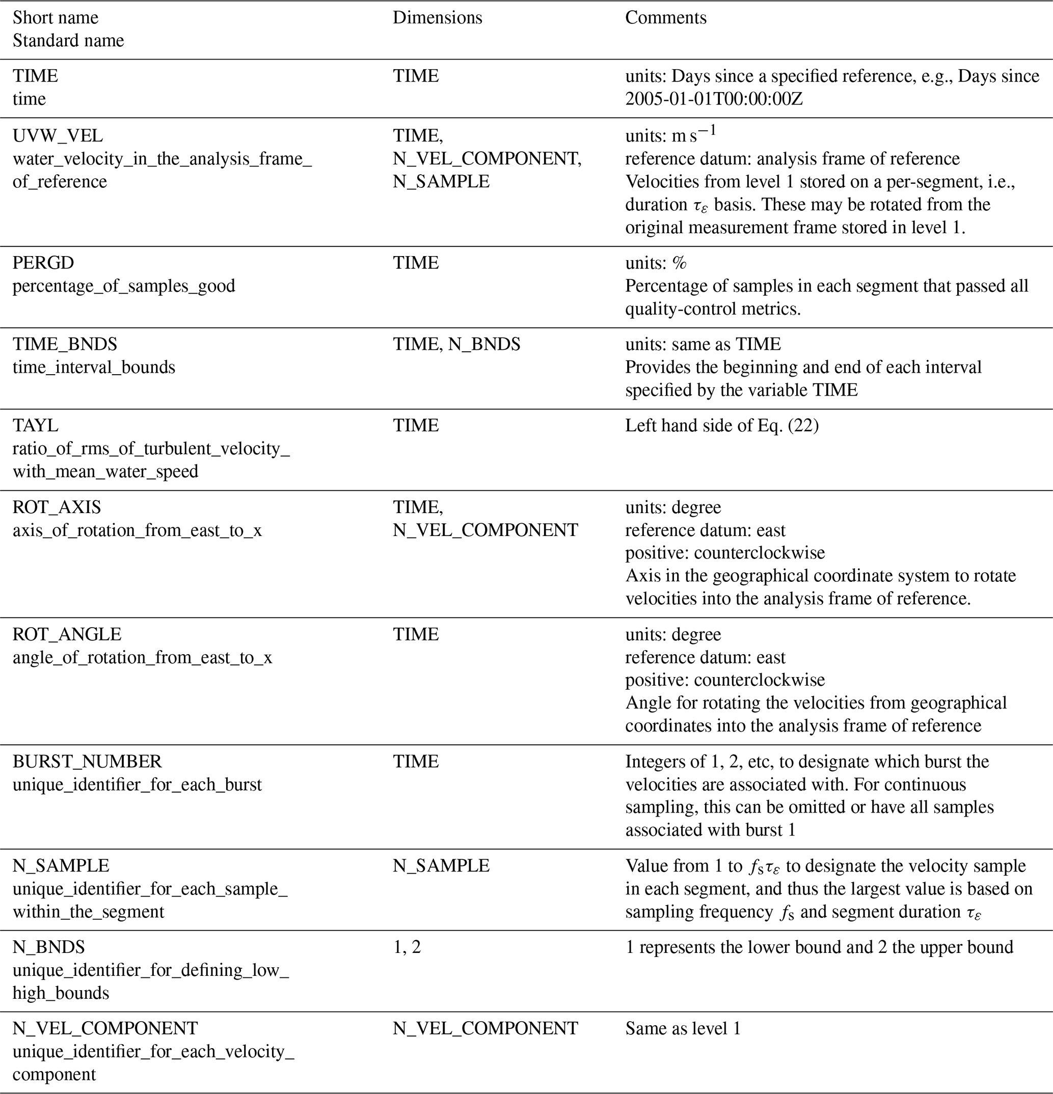
Table A3Summary of Level 3 NetCDF data format. This level includes the spectral observations.
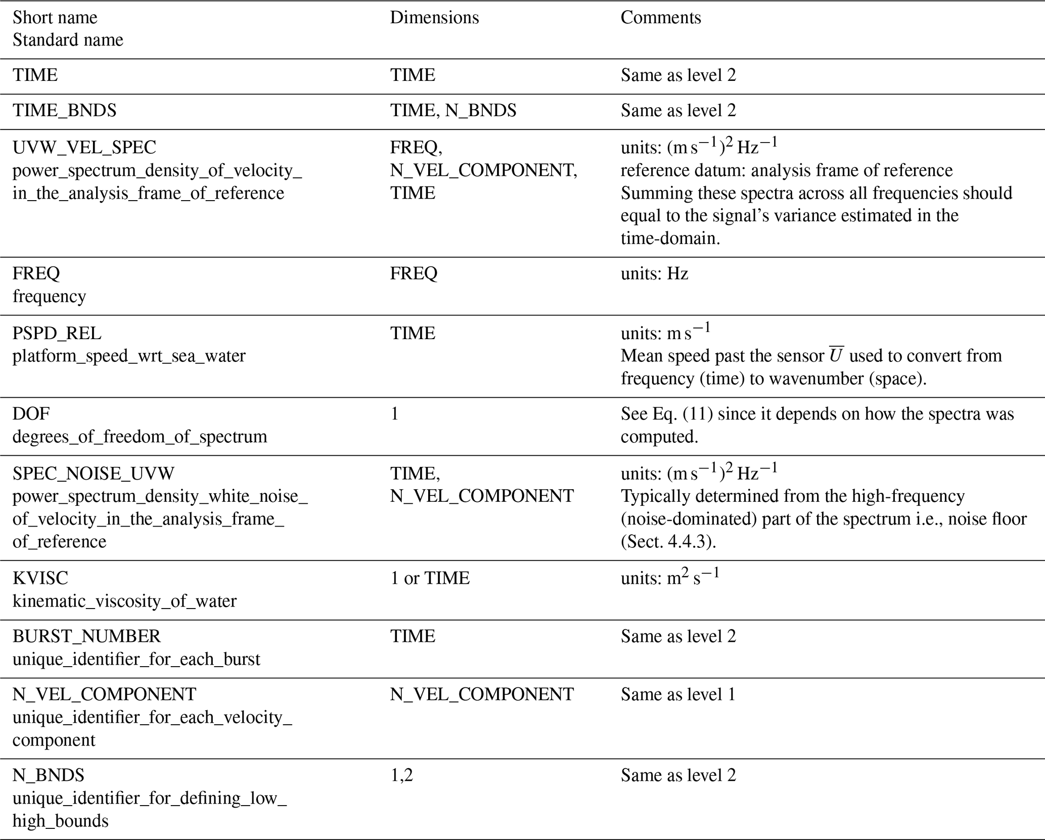
Table A4Summary of Level 4 NetCDF data format. This level includes timeseries of the dissipation estimates. The parameters necessary for re-flagging estimates are shown separately in Table A5.
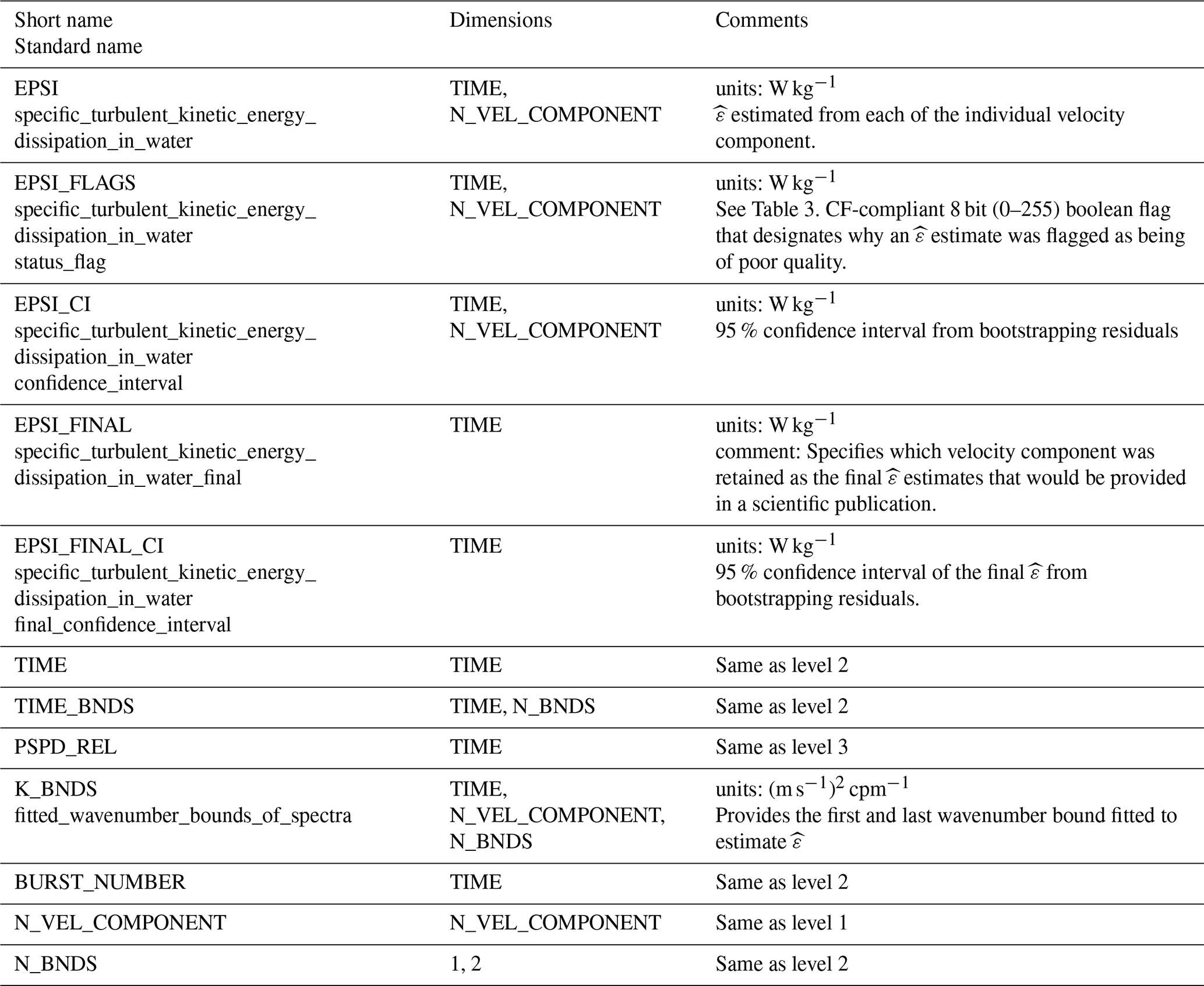
Table A5Additional parameters stored at Level 4 NetCDF for re-flagging estimates.
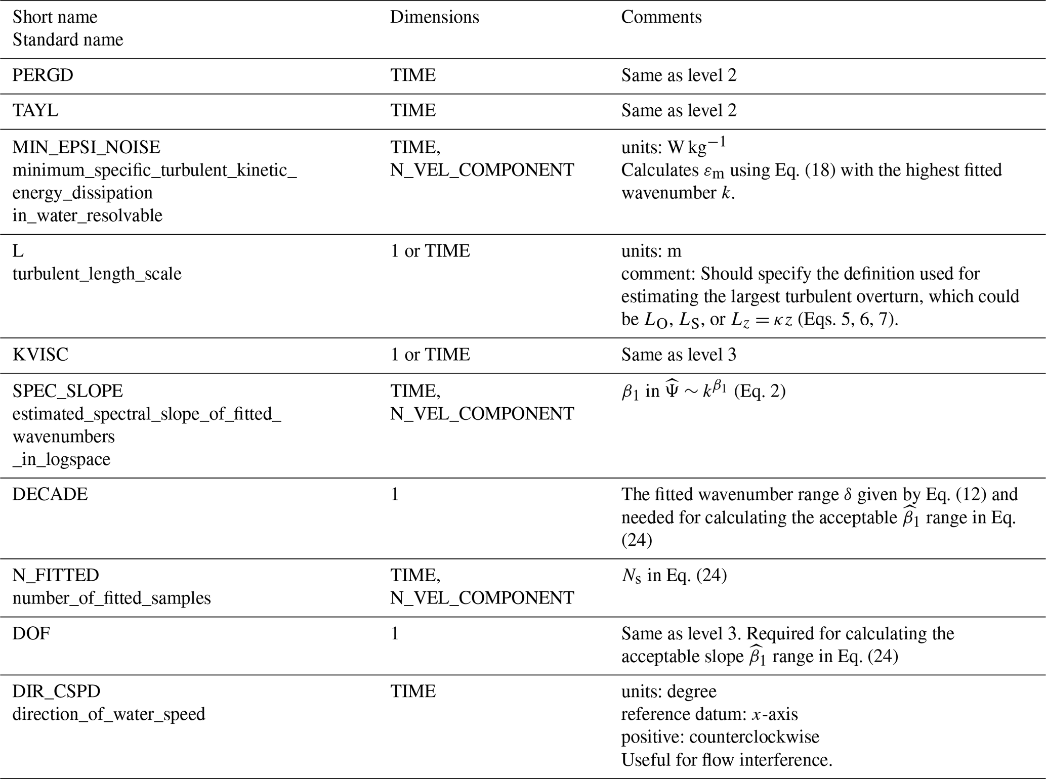
The benchmark datasets are available at the following public repository https://doi.org/10.5281/zenodo.16798905 (Bluteau et al., 2025) under the SCOR community resources. This repository also includes example templates for writing our recommended metadata into NetCDF files, along with links to tells for loading benchmarks and processing spectral observations.
Lead author CEB had primary responsibility for writing the manuscript as well as its conception. The other co-authors contributed to the following sections: Introduction – All co-authors with strong participation from CLS, DW, JM; Sects. 2 and 3 – CLS, CEB; Sect. 4 – CEB, DW, JM; Sect. 5 – CEB; Conclusion: CLS. All authors contributed to the article and approved the submitted version. CLS prepared most tables and all schematics. CEB prepared all data-centric figures. All authors critically reviewed the manuscript's scientific according to the ATOMIX working group's discussion.
The contact author has declared that none of the authors has any competing interests.
Publisher's note: Copernicus Publications remains neutral with regard to jurisdictional claims made in the text, published maps, institutional affiliations, or any other geographical representation in this paper. The authors bear the ultimate responsibility for providing appropriate place names. Views expressed in the text are those of the authors and do not necessarily reflect the views of the publisher.
These benchmarks were created according to the terms of reference of an international working group #160 ATOMIX, and the authors thank the other members of the ATOMIX working group (co-chairs Cynthia Bluteau, Ilker Fer and Yueng-Djern Lenn). The Scientific Committee on Oceanic Research funds this working group through a grant from the National Science Foundation (NSF grant #OCE-2513154) and contributions from national SCOR committees. MAVS datasets were provided by Natalie Robinson (supported by the NZ Antarctic Science Platform project ANTA1801) and Alex Hay (Tidal MAVS). The ATOMIX wiki has more information about the group's activities, and can be accessed from the working group's website: https://scor-int.org/group/analysing-ocean-turbulence-observations-to-quantify-mixing-atomix/ (last access: 11 March 2026).
This research has been supported by the Directorate for Geosciences (grant no. OCE-2140395). CS was supported by Marsden Fund awards NIW1702 and NIW2102.
This paper was edited by Karen J. Heywood and reviewed by three anonymous referees.
Bendat, J. S. and Piersol, A. G.: Random Data: Analysis and Measurement Procedures, Probability and statistics, 3rd edn., Wiley – Interscience, ISBN 0471317330, 2000. a, b
Bluteau, C.: Assessing statistical fitting methods used for estimating turbulence parameters, Limnol. Oceanogr.: Methods, https://doi.org/10.1002/lom3.10729, 2025a. a, b, c, d, e, f, g, h, i, j, k, l, m, n, o, p, q, r, s, t
Bluteau, C.: Synthetic spectra for assessing statistical fitting methods used to estimate ocean turbulence, Zenodo [data set], https://doi.org/10.5281/zenodo.10576543, 2025b. a, b, c, d, e
Bluteau, C., Stevens, C., Wain, D., and Mullarney, J.: NetCDF templates and code for creating and loading ATOMIX ADV benchmark datasets, Zenodo [data set, code], https://doi.org/10.5281/zenodo.16798905, 2025. a, b, c
Bluteau, C. E., Jones, N. L., and Ivey, G. N.: Estimating turbulent kinetic energy dissipation using the inertial subrange method in environmental flows, Limnol. and Oceanogr.: Methods, 9, 302–321, https://doi.org/10.4319/lom.2011.9.302, 2011. a, b, c, d, e, f, g, h, i
Brock, F. V.: A Nonlinear Filter to Remove Impulse Noise from Meteorological Data, Journal of Atmospheric and Oceanic Technology, 3, 51–58, https://doi.org/10.1175/1520-0426(1986)003<0051:ANFTRI>2.0.CO;2, 1986. a, b, c, d
Corrsin, S.: On local isotropy in turbulent shear flow, NACA R & M, https://ntrs.nasa.gov/citations/19930089981 (last access: 12 March 2026), 1958. a
D'Asaro, E. A.: Turbulence in the upper-ocean mixed layer, Annual Review of Marine Science, 6, 101–115, 2014. a
Davis, K. A. and Monismith, S. G.: The Modification of Bottom Boundary Layer Turbulence and Mixing by Internal Waves Shoaling on a Barrier Reef, J. Phys. Oceanogr., 41, 2223–2241, https://doi.org/10.1175/2011JPO4344.1, 2011. a, b
Davison, A. C. and Hinkley, D. V.: Bootstrap Methods and their Application, Cambridge University Press, https://doi.org/10.1017/cbo9780511802843, 1997. a, b
Fox-Kemper, B., Adcroft, A., Böning, C. W., Chassignet, E. P., Curchitser, E., Danabasoglu, G., Eden, C., England, M. H., Gerdes, R., Greatbatch, R. J., Griffies, S. M., Hallberg, R. W., Hanert, E., Heimbach, P., Hewitt, H. T., Hill, C. N., Komuro, Y., Legg, S., Le Sommer, J., Masina, S., Marsland, S. J., Penny, S. G., Qiao, F., Ringler, T. D., Treguier, A. M., Tsujino, H., Uotila, P., and Yeager, S. G.: Challenges and Prospects in Ocean Circulation Models, Front. Mar. Sci., 6, 65, https://doi.org/10.3389/fmars.2019.00065, 2019. a
Gargett, A. E., Osborn, T. R., and Nasmyth, P. W.: Local isotropy and the decay of turbulence in a stratified fluid, J. Fluid Mech., 144, 231–280, https://doi.org/10.1017/S0022112084001592, 1984. a, b, c, d
Goring, D. G. and Nikora, V. I.: Despiking acoustic Doppler velocimeter data, J. Hydraul. Eng., 128, 117–126, https://doi.org/10.1061/(ASCE)0733-9429(2002)128:1(117), 2002. a, b
Gregg, M. C.: Uncertainties and limitations in measuring ϵ and χT, J. Atmos. Oceanic Technol., 16, 1483–1490, https://doi.org/10.1175/1520-0426(1999)016<1483:UALIMA>2.0.CO;2, 1999. a
Han, N., Fan, Z., and Fang, S.: Phase unwrapping methods for solving the ambiguity in current velocity estimation based on combined signal design, Flow Measurement and Instrumentation, 59, 126–134, https://doi.org/10.1016/j.flowmeasinst.2017.12.001, 2018. a
Hay, A. E., McMillan, J. M., Cheel, R. A., and Schillinger, D.: Turbulence and drag in a high Reynolds number tidal passage targetted for in-stream tidal power, 2013 OCEANS – San Diego, 1–10, https://api.semanticscholar.org/CorpusID:39423238 (last access: 11 March 2026), 2013. a, b
Henchicks, P. J.: Comparison of turbulence measurements from a SonTek ADV and a Nobska MAVS, in: MTS/IEEE Oceans 2001. An Ocean Odyssey, Conference Proceedings (IEEE Cat. No. 01CH37295), IEEE, 3, 1860–1866, https://doi.org/10.1109/OCEANS.2001.968129, 2001. a
Ivey, G. N., Bluteau, C. E., and Jones, N. L.: Quantifying Diapycnal Mixing in an Energetic Ocean, J. Geophys. Res., 123, 346–357, https://doi.org/10.1002/2017JC013242, 2018. a
Kim, S.-C., Friedrichs, C. T., Maa, J. P.-Y., and Wright, L. D.: Estimating Bottom Stress in Tidal Boundary Layer from Acoustic Doppler Velocimeter Data, J. Hydraul. Eng., 126, 399–406, https://doi.org/10.1061/(ASCE)0733-9429(2000)126:6(399), 2000. a
Kundu, P. K.: Chapter 10 – Boundary Layers and Related Topics, in: Fluid Mechanics, edited by: Kundu, P. K., 299–348, Academic Press, San Diego, https://doi.org/10.1016/B978-0-12-428770-9.50016-1, 1990. a
Le Boyer, A., Couto, N., Alford, M. H., Drake, H. F., Bluteau, C. E., Hughes, K. G., Naveira Garabato, A. C., Moulin, A. J., Peacock, T., Fine, E. C., Mashayek, A., Cimoli, L., Meredith, M. P., Melet, A., Fer, I., Dengler, M., and Stevens, C. L.: Turbulent diapycnal fluxes as a pilot Essential Ocean Variable, Frontiers in Marine Science, 10, https://doi.org/10.3389/fmars.2023.1241023, 2023. a
Lemmin, U., Lhermitte, R., Nikora, V. I., and Goring, D. G.: ADV measurements of turbulence: can we improve their interpretation?, Journal of Hydraulic Engineering, 125, 987–988, 1999. a
Lhermitte, R. and Serafin, R.: Pulse-to-Pulse Coherent Doppler Sonar Signal Processing Techniques, Journal of Atmospheric and Oceanic Technology, 1, 293–308, https://doi.org/10.1175/1520-0426(1984)001<0293:PTPCDS>2.0.CO;2, 1984. a
Li, R., Voulgaris, G., and Wang, Y. P.: Turbulence structure and burst events observed in a tidally induced bottom boundary layer, Journal of Geophysical Research: Oceans, 127, e2021JC018036, https://doi.org/10.1029/2021JC018036, 2022. a
Lohrmann, A. and Nylund, S.: Pure coherent Doppler systems – how far can we push it?, in: 2008 IEEE/OES 9th Working Conference on Current Measurement Technology, IEEE, 19–24, https://doi.org/10.1109/CCM.2008.4480837, 2008. a, b
Lueck, R., Fer, I., Bluteau, C., Dengler, M., Holtermann, P., Inoue, R., LeBoyer, A., Nicholson, S.-A., Schulz, K., and Stevens, C.: Best practices recommendations for estimating dissipation rates from shear probes, Frontiers in Marine Science, 11, https://doi.org/10.3389/fmars.2024.1334327, 2024. a, b, c, d
Lumley, J. L.: Interpretation of Time Spectra Measured in High-Intensity Shear Flows, Phys. Fluids, 8, 1056–1062, https://doi.org/10.1063/1.1761355, 1965. a, b
Luznik, L., Gurka, R., Nimmo Smith, W. A. M., Zhu, W., Katz, J., and Osborn, T. R.: Distribution of Energy Spectra, Reynolds Stresses, Turbulence Production, and Dissipation in a Tidally Driven Bottom Boundary Layer, J. Phys. Oceanogr., 37, 1527–1550, https://doi.org/10.1175/JPO3076.1, 2007. a
Marusic, I., Monty, J. P., Hultmark, M., and Smits, A. J.: On the logarithmic region in wall turbulence, J. Fluid Mech., 716, https://doi.org/10.1017/jfm.2012.511, 2013. a
McGinnis, D. F., Sommer, S., Lorke, A., Glud, R. N., and Linke, P.: Quantifying tidally driven benthic oxygen exchange across permeable sediments: An aquatic eddy correlation study, J. Geophys. Res., 119, 6918–6932, https://doi.org/10.1002/2014JC010303, 2014. a, b
McMillan, J. M., Scannell, B., Mullarney, J. C., Wain, D. J., Lucas, N., and Lenn, Y. D.: Best practices for estimating the turbulent dissipation rate from velocity profiler measurements using structure function techniques, in preparation, 2026. a
Nortek: The Comprehensive Manual for Velocimeters, Nortek Manuals, Nortek, https://support.nortekgroup.com/hc/en-us/article_attachments/4551609336220 (last access: 12 March 2026), 2018. a
Nuttall, A. and Carter, G.: A generalized framework for power spectral estimation, IEEE Trans. Acoust., Speech, Signal Process., 28, 334–335, https://doi.org/10.1109/tassp.1980.1163412, 1980. a
Obukhov, A. M.: Turbulence in thermally inhomogeneous atmosphere, Tr. Inst. Teoret. Geofiz. Akad. Nauk SSSR, 1, 95–115, 1946. a
Ozmidov, R. V.: Energy distribution between oceanic motions of different scales, Izv. Atm. Ocean Phys., 1, 257–261, 1965. a
Pécseli, H. L. and Trulsen, J. K.: On the applicability of Taylor's hypothesis, including small sampling velocities, Journal of Fluid Mechanics, 932, A22, https://doi.org/10.1017/jfm.2021.969, 2022. a, b, c, d, e
Percival, D. B. and Walden, A. T.: Combining Direct Spectral Estimators, 351–444, Cambridge Series in Statistical and Probabilistic Mathematics, Cambridge University Press, https://www.cambridge.org/core/books/abs/spectral-analysis-for-univariate-time-series/combining-direct-spectral-estimators/675322CB191F6D4E04C919AED7008006 (last access: 12 March 2026), 2020. a, b
Pope, S. B.: Turbulent flows, 1st edn., Cambridge University Press, https://doi.org/10.1017/CBO9780511840531, 2000. a, b, c, d
Ruddick, B., Anis, A., and Thompson, K.: Maximum likelihood spectral fitting: The Batchelor spectrum, J. Atmos. Oceanic Technol., 17, 1541–1555, https://doi.org/10.1175/1520-0426(2000)017<1541:MLSFTB>2.0.CO;2, 2000. a, b
Rusello, P. J.: A Practical Primer for Pulse Coherent Instruments, Nortek technical note no.: TN-027, NortekUSA, https://support.nortekgroup.com/hc/en-us/article_attachments/360010926619 (last access: 12 March 2026), 2009. a
Rusello, P. J., Lohrmann, A., Siegel, E., and Maddux, T.: Improvements in acoustic Doppler velocimetery, ISBN 2007017155, 2006. a
Saddoughi, S. G. and Veeravalli, S. V.: Local isotropy in turbulent boundary layers at high Reynolds number, J. Fluid Mech., 268, 333–372, https://doi.org/10.1017/S0022112094001370, 1994. a, b
Shcherbina, A. Y., D'Asaro, E. A., and Nylund, S.: Observing Finescale Oceanic Velocity Structure with an Autonomous Nortek Acoustic Doppler Current Profiler, Journal of Atmospheric and Oceanic Technology, 35, 411–427, https://doi.org/10.1175/jtech-d-17-0108.1, 2018. a, b
Sreenivasan, K. R.: On the universality of the Kolmogorov constant, Phys. Fluids, 7, 2778–2784, https://doi.org/10.1063/1.868656, 1995. a, b
Starkenburg, D., Metzger, S., Fochesatto, G. J., Alfieri, J. G., Gens, R., Prakash, A., and Cristóbal, J.: Assessment of Despiking Methods for Turbulence Data in Micrometeorology, Journal of Atmospheric and Oceanic Technology, 33, 2001–2013, https://doi.org/10.1175/JTECH-D-15-0154.1, 2016. a, b, c
Stewart, R. and Grant, H.: Early measurements of turbulence in the ocean: Motives and techniques, Journal of Atmospheric and Oceanic Technology, 16, 1467–1473, 1999. a
Tercan, A. E.: Least Absolute Deviation, 1–3, Springer International Publishing, https://doi.org/10.1007/978-3-030-26050-7_176-1, 2021. a
Trowbridge, J. and Elgar, S.: Turbulence Measurements in the Surf Zone, J. Phys. Oceanogr., 31, 2403–2417, https://doi.org/10.1175/1520-0485(2001)031<2403:TMITSZ>2.0.CO;2, 2001. a
Voulgaris, G. and Trowbridge, J. H.: Evaluation of the Acoustic Doppler Velocimeter (ADV) for Turbulence Measurements, J. Atmos. Oceanic Technol., 15, 272–289, https://doi.org/10.1175/1520-0426(1998)015<0272:EOTADV>2.0.CO;2, 1998. a, b
Wyngaard, J. C. and Clifford, S. F.: Taylor's Hypothesis and High–Frequency Turbulence Spectra, J. Atmospheric Sci., 34, 922–929, https://doi.org/10.1175/1520-0469(1977)034<0922:thahts>2.0.co;2, 1977. a, b
Zheng, Z., Harcourt, R. R., and D'Asaro, E. A.: Evaluating Monin–Obukhov Scaling in the Unstable Oceanic Surface Layer, J. Phys. Oceanogr., 51, 911–930, https://doi.org/10.1175/jpo-d-20-0201.1, 2021. a
Zippel, S. F., Farrar, J. T., Zappa, C. J., Miller, U., Laurent, L. S., Ijichi, T., Weller, R. A., McRaven, L., Nylund, S., and Bel, D. L.: Moored Turbulence Measurements Using Pulse-Coherent Doppler Sonar, Journal of Atmospheric and Oceanic Technology, 38, 1621–1639, https://doi.org/10.1175/JTECH-D-21-0005.1, 2021a. a
Zippel, S. F., Farrar, J. T., Zappa, C. J., Miller, U., Laurent, L. S., Ijichi, T., Weller, R. A., McRaven, L., Nylund, S., and Le Bel, D.: Moored Turbulence Measurements using Pulse-Coherent Doppler Sonar, Journal of Atmospheric and Oceanic Technology, https://doi.org/10.1175/jtech-d-21-0005.1, 2021b. a
- Abstract
- Introduction
- Background theory and sampling requirements
- Benchmark datasets and formatting
- Processing methods
- Application of methods to benchmark datasets
- Conclusions
- Appendix A: NetCDF variable names
- Code and data availability
- Author contributions
- Competing interests
- Disclaimer
- Acknowledgements
- Financial support
- Review statement
- References