Tidal signatures on surface chlorophyll a concentration in the Brazilian Equatorial Margin

This study investigates the influence of tides on chlorophyll a (CHL) variability in the Brazilian Equatorial Margin using daily GlobColour and MODIS-Aqua CHL data from 2005 to 2021. The impact of the tides is assessed by comparing the spring with the neap tide signals (fortnightly signal, 14.7 d). Results show that, on the shallow Amazon shelf, significant fortnightly CHL variability is likely primarily driven by barotropic tide-induced friction on the shelf that produces significant vertical mixing. On the northwestern shelf, where the Amazon River plume prevails, CHL levels are higher during neap tides, resulting in a negative spring–neap tide CHL difference (GlobColour: −50 %; MODIS-Aqua: −84 %). Conversely, on the northeastern shelf, characterized by low-turbidity waters, CHL levels are higher during spring tides, leading to a positive spring–neap tide CHL difference (GlobColour: +30 %; MODIS-Aqua: +70 %). Offshore, baroclinic tides, also known as internal tides (ITs), seem to enhance the CHL along their pathways with a spatial structure of a wave-like pattern. The positive CHL peaks are spaced by mode-2 wavelengths (about 68 km), with peak values reaching +3.3 % (GlobColour) and +9.0 % (MODIS-Aqua). Analysis shows that the CHL wave-like pattern suggests contributions from mode-1 and mode-2 internal tides, with mode-2 components having higher spectral coherence with the original signal. A 1–3 d lag between higher CHL variability and tidal potential may indicate delayed nutrient mixing post-spring–neap tides. The effects of ITs on CHL are more pronounced than on sea surface temperature.

1 Introduction

The Brazilian Equatorial Margin (BEM) is characterized by intense activity of internal tides (ITs) (Tchilibou et al., 2022), also known as baroclinic tides. The seasonal variability in water stratification, currents, and mesoscale circulation significantly influences IT activity in this region. From March to July, the pycnocline is shallower, slightly stronger, and more horizontally homogeneous, along with weaker currents and reduced mesoscale activity (Richardson and Walsh, 1986; Richardson et al., 1994; Silva et al., 2005; Aguedjou et al., 2019; Tchilibou et al., 2022; Assene et al., 2024). Between August and December, the pycnocline becomes deeper and slightly weaker, the North Equatorial Countercurrent (NECC) intensifies, and the eddy kinetic energy (EKE) increases, leading to longer IT wavelengths (Barbot et al., 2021; Tchilibou et al., 2022). See the overview of the study area in Fig. 1.

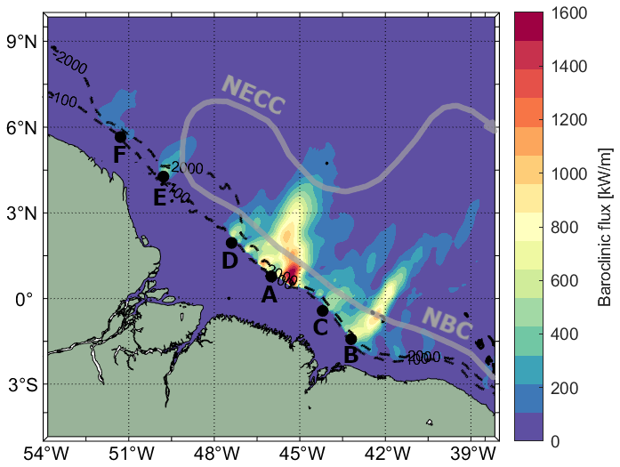
Figure 1 Baroclinic flux over the BEM. IT generation sites are labeled from A to F along the shelf break. The black dashed line and black dots represent the bathymetric contours of −100 and −2000 m, and the generation points, respectively, following Assene et al. (2024). The North Brazil Current (NBC) and the NECC are highlighted with thick gray arrows.

The BEM is also known for intense activity of internal solitary waves (ISWs). Magalhaes et al. (2016) show that the ISWs off the Amazon shelf originate from the disintegration of ITs occurring several hundred kilometers from their generation sites along the steep Amazon shelf break. During the months from August to December, the combined effect of stronger background currents and a deeper, less stratified pycnocline leads to greater variability and longer mean ISW wavelengths (Magalhaes et al., 2016; de Macedo et al., 2023). Furthermore, de Macedo et al. (2023) found that ISW activity in the region is greater during spring tides than neap tides.

Mixing induced by tides can significantly affect water mass formation and properties, influencing primary production and water temperature (da Silva et al., 2002; Koch-Larrouy et al., 2007; Hu et al., 2008; Sharples, 2008; Muacho et al., 2014; González-Haro et al., 2019; Kossack et al., 2023; Assene et al., 2024; Jacobsen et al., 2023; Capuano et al., 2025; M'hamdi et al., 2025). The strong ITs off the Amazon shelf can induce vertical mixing by dissipating part of their energy locally at the shelf break, as well as along their propagation path, with maximum dissipation occurring approximately every 120 km, corresponding to the mode-1 wavelength (Tchilibou et al., 2022; Assene Mvongo, 2024). Assene Mvongo (2024) show that the offshore mixing along the IT propagation path can cause sea surface temperature (SST) to cool up to 0.3 °C with a higher cooling in the thermocline up to 1.2 °C.

According to da Silva et al. (2002), as interfacial ITs propagate (i.e., IT waves that propagate horizontally along density interfaces), they cause vertical displacements in the pycnocline and hence displace passive phytoplankton cells within the water column. This movement shifts the deep chlorophyll maximum (DCM) either above or below the light penetration depth, resulting in, respectively, increased or decreased chlorophyll a concentrations (hereinafter referred to as CHL) detected by remote sensing (da Silva et al., 2002; Muacho et al., 2014; Kim et al., 2018; M'hamdi et al., 2025). According to Lande and Yentsch (1988) and Jacobsen et al. (2023), the vertical displacement of phytoplankton by ITs can alter the light available for primary production.

Additionally, ITs enhance the vertical mixing of nutrients into the DCM, thus supporting primary production (Sharples et al., 2007; Tuerena et al., 2019; Kossack et al., 2023; Jacobsen et al., 2023). Jacobsen et al. (2023) studied the response of primary production to IT beams based on model simulations configured for an oligotrophic system with a nutricline depth below 50 m. They found that while subsurface light limitation is reduced for passive plankton within tidal beams, leading to higher primary production rates, the dominant effect of tidal beams on primary production is the increased nutrient supply to the euphotic zone near tidal beam generation locations. M'hamdi et al. (2025) demonstrated using a Slocum G2 glider deployed off the Amazon shelf during AMAZOMIX 2021 cruise that the enhancement of the CHL concentration associated with the passage of ITs may be due to two combined effects: (1) the ITs modulate the DCM, causing its vertical displacement and oscillation as it rises and deepens in response to IT propagation. This movement may enhance phytoplankton's light exposure, stimulating primary production; (2) mixing events associated with ITs increase CHL concentration in both the surface and bottom layers of the water column.

In shallow coastal waters, barotropic tides primarily dissipate their energy through friction with the seabed, generating bottom-driven mixing that alters water properties. This mixing can enhance primary production by replenishing nutrients in the surface mixed layer (Hu et al., 2008; Sharples, 2008). However, this shelf mixing can also inhibit phytoplankton growth by promoting resuspended sediments, which reduces the photosynthetically available radiation (PAR) (Byun et al., 2007; Xing et al., 2021; Kossack et al., 2023).

Tides are characterized by spring–neap tidal cycles (fortnightly cycles, approximately 14.77 d), which impact water mass properties. According to Sharples (2008), the fortnightly modulation of tidal mixing affects time and magnitude of primary production in stratified shelf areas; changes in the timing of the spring–neap cycle could account for up to 10 % of the total inter-annual variability of bloom timing in regions with weak tidal regimes, and up to 25 % in areas with stronger tidal currents. In the region of the Indonesian Throughflow, fortnightly variations in chlorophyll (CHL) concentration in shallow coastal waters have been attributed to the spring–neap cycle of barotropic ocean currents (Zaron et al., 2023; Capuano et al., 2025). In deeper waters, the authors hypothesized that the fortnightly CHL variability is linked to the modulation of vertical nutrient fluxes by baroclinic tidal mixing. Sharples et al. (2007) observed that in a stratified water column of 200 m depth at the shelf edge of the Celtic Sea, the upward mixing of nutrients across the thermocline, driven by an internal tide, resulted in a much higher nitrate flux into the surface layer during the spring tide than during the neap tide, thereby fueling new primary production. In the northwestern Amazon shelf, Assene Mvongo (2024) found maximum values of fortnightly temperature variability (∼0.15 °C). The author showed that the fortnightly modulation of temperature is enhanced in the thermocline with a horizontal structure similar to the baroclinic Sea Surface Height (SSH) along IT pathways. Authors also noted a 2–3 d delay between the astronomical tidal forcing and the peak of temperature variability.

Despite the advances made so far, significant gaps remain concerning the impact and spatial extent of tides (particularly baroclinic tides) on CHL concentration and SST in the BEM. In this study, we investigate the fortnightly signal in remote sensing surface CHL concentration, accounting for various delays related to astronomical tidal forcing. To our knowledge, this is the first time that the influence of baroclinic tides on CHL concentration has been demonstrated in the BEM using a long-term remote sensing time series.

2 Data and methods

2.1 Remote sensing data processing

ISW signatures were identified in two illustrative images acquired on 28 September 2007 and 12 October 2018, over the Amazon shelf in the region of sunglint. These images consist of Level 1B data from the Moderate Resolution Imaging Spectroradiometer (MODIS) sensor onboard the TERRA satellite, using band 6 (centered at 1640 nm) with a spatial resolution of 500 m. The MODIS-Terra images were obtained from NASA's Earth Science Data System (ESDS) (https://doi.org/10.5067/MODIS/MOD02QKM.NRT.061 MODIS Science Team, 2017).

CHL data were derived from daily Level 1A acquisitions of the Moderate Resolution Imaging Spectroradiometer (MODIS) onboard the Aqua satellite, covering the period from 1 January 2005 to 31 December 2021, at a spatial resolution of 1 km. The Level 1A MODIS-Aqua images were obtained from NASA's Ocean Color website (https://oceancolor.gsfc.nasa.gov/, last access: 13 December 2023) and processed to Level 1C using the SeaDAS 8.1.0 software package (https://seadas.gsfc.nasa.gov/, last access: 1 December 2022). Remote sensing reflectance (Rrs) was computed from the Level 1C MODIS data using POLYMER 4.13 (https://www.hygeos.com/polymer, last access: 1 December 2022) for atmospheric correction. POLYMER is specifically designed to recover marine reflectance and is particularly effective in correcting for effects of sunglint (Steinmetz et al., 2011). Rrs values were then used to estimate near-surface CHL concentrations through NASA's standard algorithm implemented in SeaDAS. This algorithm combines an updated version of the OC3M band ratio algorithm (O'Reilly and Werdell, 2019) with the color index (CI) approach (Hu et al., 2019).

Since the study area is highly affected by clouds throughout the year, we have used as well the daily L4 CHL data from the global multi-sensor Copernicus-GlobColour processor, which is a blend between OC5 (Gohin et al., 2002) and CI of Hu et al. (2012). The GlobColour product was obtained from the Copernicus Marine Service (https://doi.org/10.48670/moi-00281 Copernicus Marine Service, 2023a) for the period from 1 January 2005 to 31 December 2021, at a spatial resolution of 4 km. This product is a CHL daily composite obtained by merging multiple ocean satellite sensor acquisitions (SeaWiFS, MODIS, MERIS, VIIRS-SNPP, JPSS1, OLCI-S3A, and S3B) and by applying temporal averaging and interpolation methods to fill the missing data values.

Models based on band ratios in the visible spectrum offer reliable chlorophyll estimates for clear to moderately turbid waters but show limitations in highly turbid environments (Tran et al., 2023). Considering the presence of highly turbid waters in our study area, associated with the Amazon River plume, we applied the methodology developed by Tran et al. (2023) to exclude information from highly turbid locations. Specifically, if a given location (longitude, latitude) was classified as turbid waters (optical water types 4 and/or 5) in more than 20 % of the time series, all data from that location were excluded from the analysis. This approach helped avoid bias in the time series by removing pixels that were permanently or episodically associated with turbid environments. Overall, the excluded pixels are mainly confined to areas shallower than 100 m, where there is no evidence the ISWs discussed in this manuscript.

Gap-free maps of daily L4 foundation sea surface temperature (SST) data from the OSTIA were acquired from 1 January 2007 to 31 December 2021 in the Copernicus Marine Service (Stark et al., 2007; Donlon et al., 2012; Good et al., 2020) (https://doi.org/10.48670/moi-00165). This product uses in-situ data and merged satellite observations (AMSR2-GCOM-W, AVHRR-MetOp-B, SEVIRI-MSG, VIIRS-SNPP, NOAA-20, SLSTR-S3A, and S3B) and provides SST maps at 0.05°×0.05°. horizontal grid resolution.

2.1.1 IT illustrative case analysis

The presence of ISW signatures in two MODIS-Terra images acquired under conditions of sunglint over the BEM is used as a proxy for IT activity. To emphasize the impact of ITs on the CHL concentration, we calculated the CHL relative difference at pixel p (in %), ΔCHL_p, defined as the deviation between the CHL concentration on the day when ISW signatures were detected (i.e., the illustrative case day) and the 15 d mean CHL values centered on that day:

$$\begin{array}{}\text{(1)}& \mathrm{\Delta }{\mathrm{CHL}}_{\mathrm{p}}\left(\mathit{\%}\right)={\displaystyle \frac{{\mathrm{CHL}}_{\mathrm{p},\mathrm{0}}-\stackrel{\mathrm{‾}}{{\mathrm{CHL}}_{\mathrm{p}}}}{\stackrel{\mathrm{‾}}{{\mathrm{CHL}}_{\mathrm{p}}}}}\times \mathrm{100}\end{array}$$

where

$$\begin{array}{}\text{(2)}& \stackrel{\mathrm{‾}}{{\mathrm{CHL}}_{\mathrm{p}}}={\displaystyle \frac{\mathrm{1}}{\mathrm{15}}}\sum _{i=-\mathrm{7}}^{+\mathrm{7}}{\mathrm{CHL}}_{\mathrm{p},i}.\end{array}$$

CHL_p,i is the CHL concentration at pixel p on day i (with i=0 the illustrative case day, i=−7 the 7th day before, and $i=+\mathrm{7}$ the 7th day after). This enables the assessment of potential changes in CHL concentrations driven by ITs, compared to the CHL 15 d average within the study area.

2.2 Wavelet analysis

In regions where M2 and S2 tidal constituents dominate, their nonlinear interaction generates the MSf (Lunisolar Synodic Fortnightly) oscillation, with a period of approximately 14.7 d. The MSf corresponds to the neap–spring tidal cycle, a phenomenon of great importance in tidal dynamics and a major physical factor influencing coastal and marine environments. Wavelet analysis was therefore applied to identify and quantify this fortnightly variability in the CHL and SST time series. This approach is a powerful tool for analyzing ecological systems since the methodology performs a local time-scale decomposition of the signal overcoming the problem of non-stationarity in time series (Lau and Weng, 1995; Torrence and Compo, 1998; Cazelles et al., 2008). The 1D continuous wavelet spectral analysis was carried out on daily CHL GlobColour and OSTIA products. The continuous Morlet wavelet transform was applied to the CHL and SST anomaly time series, which was performed using Python 3.8 and the free Python package PyCWT (https://pypi.org/project/pycwt/, last access: 24 January 2024) based on the method developed in Torrence and Compo (1998). The power spectra significance test was made according Torrence and Compo (1998). Xing et al. (2021) applied a similar wavelet approach to investigate CHL variability associated with spring–neap tidal cycles.

2.3 Spring–neap tidal cycle composite

We developed an alternative methodology to investigate the fortnightly tidal modulation of CHL by constructing spring–neap tidal cycle composite maps. Assuming the IT signal is coherent (i.e., coherent ITs), these composites can resolve the broader MSf frequency. Unlike wavelet analysis or other commonly applied methods to examine IT-related frequency content (e.g., least-squares harmonic analysis; Zaron et al., 2023), our approach also preserves the sign of spring–neap CHL variability. This enables us to determine whether tidal influences at the MSf frequency drive increases or decreases in CHL concentration within the affected region. If the IT signal is incoherent, however, this method is unlikely to extract the MSf frequency reliably.

Tidal elevation at the Amazon shelf break (45.5° W, 1° N) was analyzed using the Tidal Toolbox, available within the COMODO tools developed and maintained by the SIROCCO (SImulation Réaliste de l'OCéan COtier) national service (https://sirocco.obs-mip.fr/other-tools/prepost-processing/comodo-tools/, last access: 6 July 2023).

Let S and N denote the CHL concentrations at the maximum and minimum tidal range elevation, respectively, spring and neap tidal cycles during the time series period (please, see Fig. 2). The composite maps, i.e., the weighted spring-minus-neap CHL difference for pixel p, f_p(S,N), averaged over all cycles, can be calculated as follows:

$$\begin{array}{}\text{(3)}& \begin{array}{rl}& f_{\mathrm{p}}(S,N)={\displaystyle \frac{\mathrm{1}}{n}}\sum _{i=\mathrm{1}}^n\\ & {\displaystyle \frac{\left(\frac{\mathrm{3}}{\mathrm{4}}{S}_{\mathrm{p},i}^{\left(w\right)}+\frac{\mathrm{1}}{\mathrm{4}}{S}_{\mathrm{p},i+\mathrm{1}}^{\left(w\right)}\right)-\left(\frac{\mathrm{1}}{\mathrm{4}}{N}_{\mathrm{p},i}^{\left(w\right)}+\frac{\mathrm{3}}{\mathrm{4}}{N}_{\mathrm{p},i+\mathrm{1}}^{\left(w\right)}\right)}{\stackrel{\mathrm{‾}}{{\mathrm{CHL}}_{\mathrm{p},i}}}}\end{array}\end{array}$$

where

$$\begin{array}{}\text{(4)}& S_{\mathrm{p},i}^{\left(w\right)}={\displaystyle \frac{\mathrm{1}}{\mathrm{3}}}\sum _{j=-\mathrm{1}}^{+\mathrm{1}}{S}_{\mathrm{p},t_{\mathrm{S}},i+j},N_{\mathrm{p},i}^{\left(w\right)}={\displaystyle \frac{\mathrm{1}}{\mathrm{3}}}\sum _{j=-\mathrm{1}}^{+\mathrm{1}}{N}_{\mathrm{p},t_{\mathrm{N}},i+j}\end{array}$$

$S_{\mathrm{p},t_{\mathrm{S}},i+j}$ ($N_{\mathrm{p},t_{\mathrm{N}},i+j}$) is the CHL value at pixel p on day $t_{\mathrm{S},i}+j$ ($t_{\mathrm{N},i}+j$), where t_S,i (t_N,i) is the nominal day of the ith spring (neap) tide event, i.e., and j=0, $j\mathit{ϵ}\mathit{\{}-\mathrm{1},\mathrm{0},+\mathrm{1}\mathit{\}}$ days from spring tides. CHL_p,i represents the mean CHL concentration used to normalize each spring-minus-neap CHL difference in the series. Specifically, for each index i, CHL_p,i is computed as the average of all CHL values included in the calculation of the weighted difference, considering both the spring and neap tide observations within the local 3-pixel window. This normalization allows each difference to be expressed relative to the local CHL magnitude, ensuring comparability across the time series. In addition to the composite map centered on the spring and neap tide events, we also computed alternative composites by introducing temporal lags. This approach accounts for the phase lag between the maximum tidal potential and the maximum tidal elevation (the so-called age of the tide), when mixing intensity typically peaks. Specifically, we considered delayed versions of spring and neap tides, defined as $S=\mathit{\left\{}{S}_{\mathrm{p},i+\mathrm{delay}}\mathit{\right\}}$ and $S=\mathit{\left\{}{S}_{\mathrm{p},i+\mathrm{delay}}\mathit{\right\}}$, where $\mathrm{delay}=\mathit{\{}\mathrm{0},\mathrm{1},\mathrm{2},\mathrm{3},\mathrm{4},\mathrm{5}\mathit{\}}$ days.

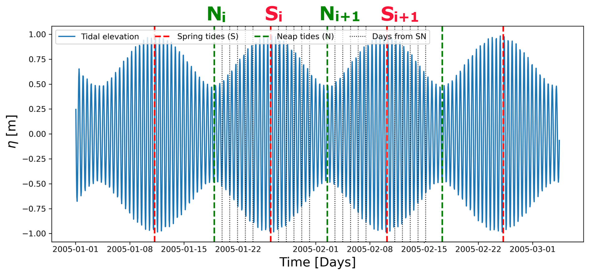
Figure 2 Tidal elevation analysis using the COMODO tools with the Spring-Neap modulation (∼14–15 d) at the Amazon shelf break [45.5° W, 1° N]. The red and green dashed lines indicate the times of spring and neap tides, respectively. The black dotted lines represent the days between consecutive spring and neap tides.

3 Results

3.1 IT illustrative case analysis

We investigated daily CHL data in the BEM derived from MODIS-Aqua and GlobColour data for days when ISWs signatures were identified in MODIS-Terra images acquired under sun glint conditions (de Macedo et al., 2023). The presence of ISWs is used as a proxy for the presence of ITs. We selected two illustrative cases to demonstrate how the passage of ITs can influence chlorophyll concentration, thereby justifying the subsequent analysis that extrapolates this effect to a 17-year time series. It is important to note that, although these cases exhibit chlorophyll modulation patterns previously associated with ITs in other studies (da Silva et al., 2002; Muacho et al., 2014), they are not necessarily representative of the typical conditions in our study area, particularly given the lack of data during months with high cloud coverage (from January to July). Furthermore, an examination of the background circulation and sea level anomaly (see Fig. A1) for the days corresponding to the illustrative cases reveals that eddy activity is more intense during illustrative case I. However, in both periods, the ISW location remains outside and to the south of the region directly influenced by the mesoscale processes.

In both illustrative cases, the MODIS-Aqua images were captured 2.55 h after the MODIS-Terra ones, corresponding to a northeastward displacement of approximately 25 km in the ISW location. Figures 3 and 4 present these illustrative cases, with the leading waves of the ISW indicated by dotted-dashed black lines. The wave positions depicted have not been adjusted for their displacement between the two remote sensing image acquisitions.

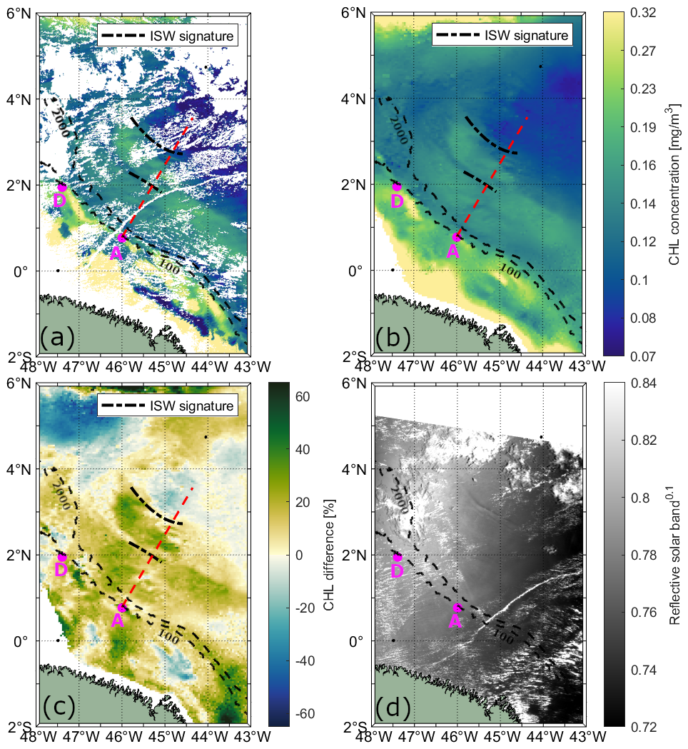
Figure 3 Illustrative case I showing the influence of ITs on CHL concentration on 28 September 2007. CHL concentration data is shown from (a) MODIS-Aqua and (b) Globcolour product. (c) CHL relative difference (%) between the CHL on the day of ISW occurrence and the 15 d mean CHL centered on that day (see, Eq. 1) from GlobColour product. (d) ISW signatures observed in the MODIS-Terra image. The red dashed line and magenta dots indicate the IT pathway and generation points, respectively, based on Assene et al. (2024). Black dashed lines mark the ISW signatures visible in the MODIS-Terra image.

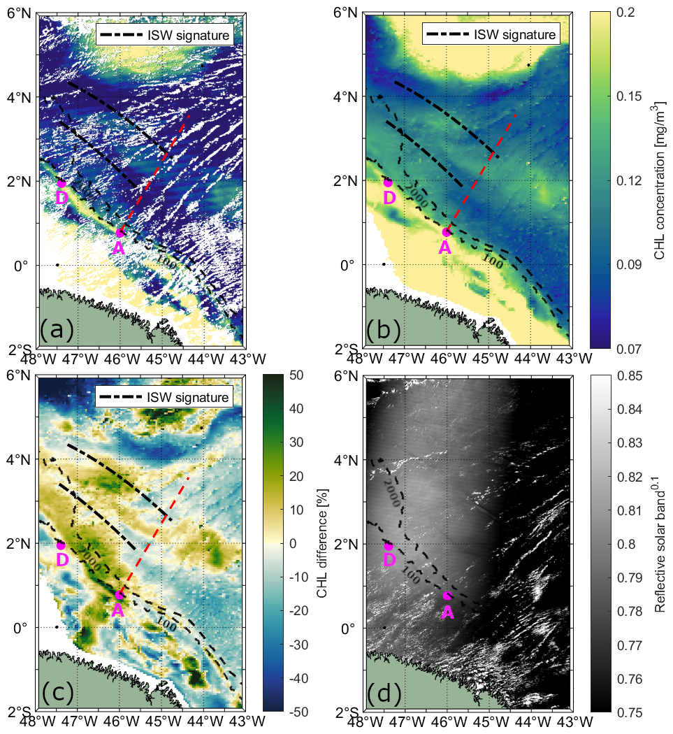
Figure 4 Illustrative case II showing the influence of ITs on CHL concentration on 12 October 2018. CHL concentration data is shown from (a) MODIS-Aqua and (b) Globcolour product. (c) CHL relative difference (%) between the CHL on the day of ISW occurrence and the 15 d mean CHL cente on that day (see, Eq. 1) from GlobColour product. (d) ISW signatures observed in the MODIS-Terra image. The red dashed line and magenta dots indicate the IT pathway and generation points, respectively, based on Assene et al. (2024). Black dashed lines mark the ISW signatures visible in the MODIS-Terra image.

For illustrative case I, shown in Fig. 3a and b, daily CHL levels retrieved from MODIS-Aqua and GlobColour are displayed, respectively. On the left side of the IT pathway A (indicated by the red dashed line), two bands of elevated CHL concentration are visible, extending parallel to the shelf break between IT generation sites A and D. The bands are separated by approximately 100 km, typical mode-1 IT wavelengths (150–100 km). In the location of the mapped ISW leading wave, CHL concentration is similar to the background levels. The offshore band of enhanced CHL (around 2.5° N, 45.5° W) is flanked by two ISW signatures. On the right side of IT pathway A, we also observe bands of elevated CHL concentration separated by about 68 km, typical mode-2 IT wavelengths. In illustrative case II (Fig. 4a and b), a similar modulation of CHL concentration is evident, with the offshore band of elevated CHL also being flanked by ISW signatures. The positions of the enhanced chlorophyll bands in illustrative case II closely match those in illustrative case I. Furthermore, although the CHL concentration is generally higher in the GlobColours product for both illustrative cases, the spatial patterns in both products show agreement.

For illustrative cases I and II, CHL concentration values along IT pathway A, derived from MODIS-Aqua and GlobColour data, are shown in Figs. 5a, c and 5b, d, respectively. When ISW signatures cross the IT pathway, their positions are marked as vertical dashed magenta lines on the graph. Accounting for the displacement of the waves from different scene acquisitions, the recalculated wave position is indicated by a vertical dashed cyan line for the MODIS-Aqua CHL data. The recalculated position is not plotted for GlobColour because its exact acquisition time is unknown, as it is a merged product (without a defined acquisition time). In both illustrative cases, a distinct peak in the CHL concentration profile is observed at 262 km (202 km from the IT generation point A), with the peak being more pronounced in illustrative case I when considering the MODIS-Aqua data.

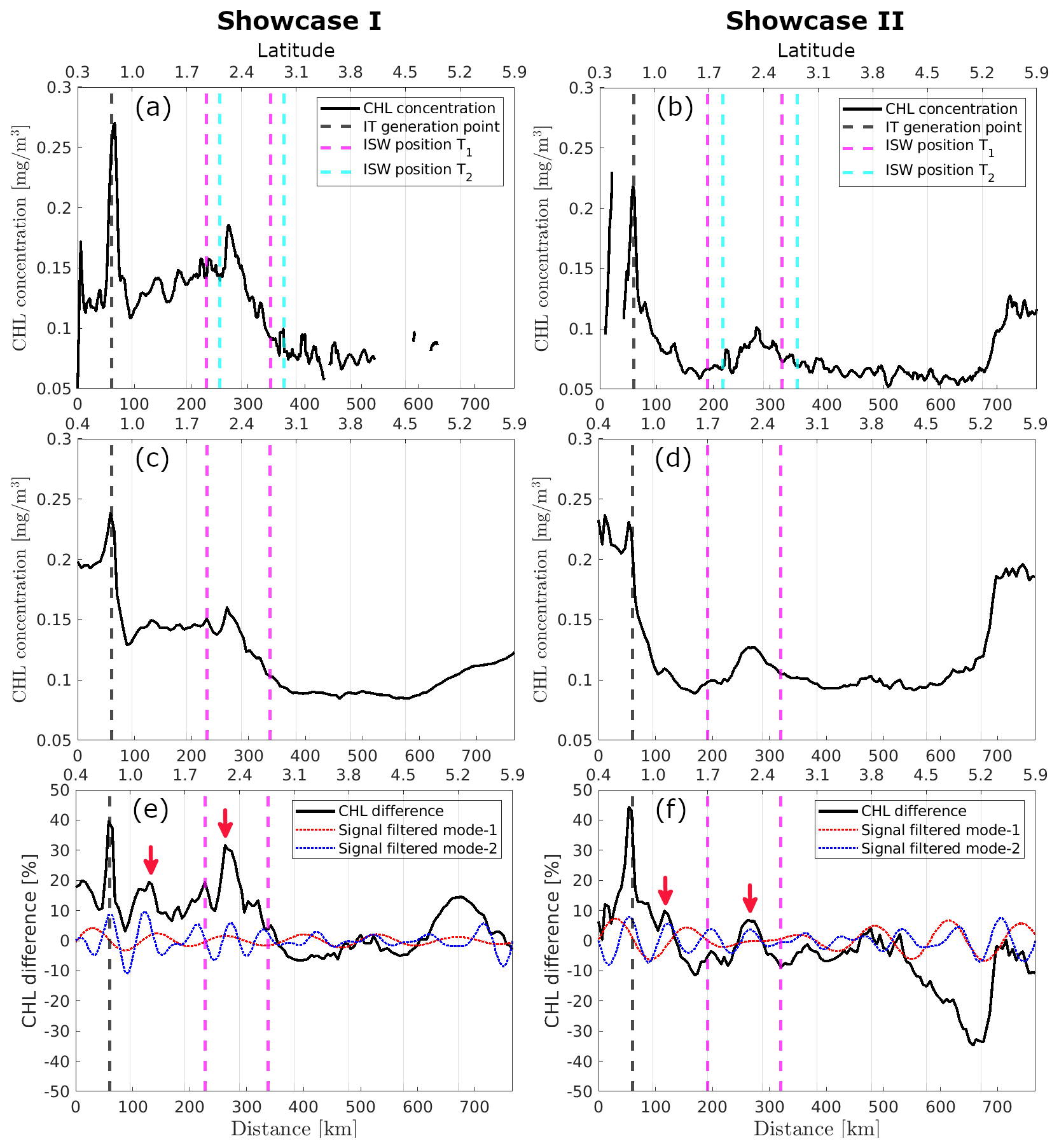
Figure 5 CHL concentration data along IT pathway A is shown from MODIS-Aqua for illustrative cases (a) I and (b) II, and from the GlobColour product for illustrative cases (c) I and (d) II. CHL relative difference is presented for illustrative cases (e) I and (f) II.

The maps of CHL relative difference are shown for illustrative cases I and II in Figs. 3c and 4c, respectively. In both illustrative cases, the bands of enhanced CHL correspond to concentrations higher than the 15 d average. Figure 5e and f depicts the chlorophyll relative differences along IT pathway A for both illustrative cases. In both instances, a pronounced CHL relative difference peak of up to 45 % is observed at the IT generation site A. For illustrative case I, two peaks in CHL difference along path A are observed at approximately 129 and 262 km (respectively, 69 and 202 km from IT generation point A, see red arrows), with the first peak reaching 19 % and the second up to 31 %. For illustrative case II, two peaks are found at 122 km (8 %) and 262 km (7 %), respectively, 62 and 202 km from the IT generation site A. A 1D horizontal band-pass filter for mode-1 and mode-2 wavelength (respectively, 100–150 and 50–100 km, see red and blue dashed lines in Fig. 5e and f) was applied to highlight the impact of the IT. For each transect, the mean spectral coherence (Rabiner and Gold, 1975; Kay, 1988; Welch, 1967) between the original CHL relative difference signal and the band-pass filter components (mode-1 and mode-2) was computed to quantify the relative contribution of each internal tide mode. For illustrative case I, the mean spectral coherence values for mode-1 and mode-2 are 0.11 and 0.23, respectively, suggesting that mode-1 and mode-2 tides contribute approximately 11 % and 23 % of the observed signal. For case II, the corresponding values are 0.17 and 0.26, indicating contributions of about 17 % and 26 %, respectively. Modulations are stronger and more coherent with the original signal when considering the signal filtered for mode-2 wavelength in both cases, with the offshore signal weakening beyond the first 300–400 km.

3.2 Wavelet analysis

Figure 6a shows the spatial variability of the fortnightly signal in the gap-free GlobColour CHL product, extracted using the mean Morlet wavelet power within the 14.2 to 15.2 d period where the power was statistically significant above the 95 % confidence for red noise. The SST fortnightly signal was calculated using the same methodology (see Fig. 6b). The depth-integrated barotropic and baroclinic energy flux (black arrows) and dissipation from Assene et al. (2024), computed using the Nucleus for European Modeling of the Ocean (NEMO v4.0.2, Madec et al., 2024) with the AMAZON36 configuration, are shown in Fig. 6c and d, respectively. For both CHL and SST, the fortnightly signal is more intense in the northwest part of the shelf region around 46.5–52° W and 0–6° N, where barotropic tides dissipate through bottom friction, see Fig. 6c. Offshore, the highest values of the CHL fortnightly signal are mostly concentrated in the northwest part while, for SST, the fortnightly signal considerably reduces. Areas with high CHL fortnightly power can also be seen aligned with the IT pathways A, B, and C (see the gray dashed rectangles in Fig. 6a). The areas of high power along IT pathways A and B align well with the lower values of depth-integrated S2 baroclinic energy dissipation predicted by the model.

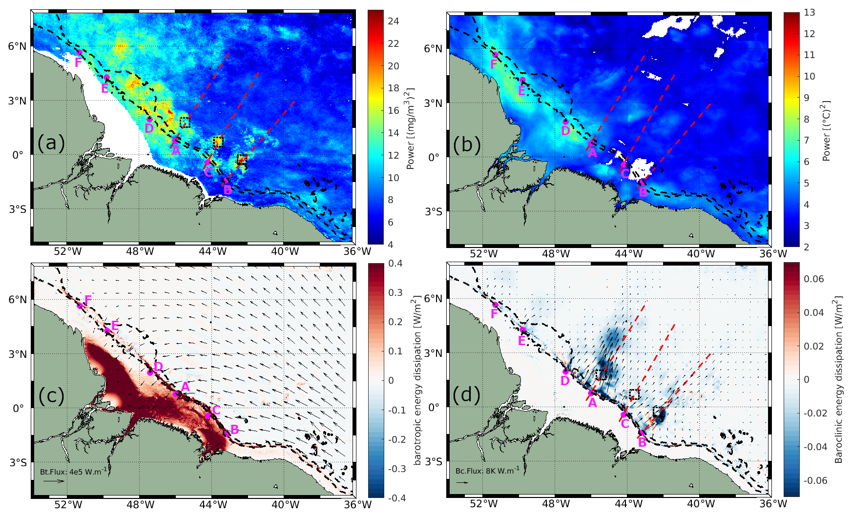
Figure 6 Mean Morlet wavelet power for periods between 14.2 and 15.2 d is shown for (a) CHL and (b) SST. Depth-integrated (c) barotropic and (d) baroclinic energy fluxes are represented by black arrows, with dissipation values calculated from AMAZON36. Black dashed rectangles indicate areas of high CHL fortnightly power, IT generation points identified are marked in magenta, and IT pathways are depicted by red dashed lines (Assene et al., 2024).

3.3 Spring–neap tidal cycle composite

Figure 7 presents the CHL spring–neap tidal cycle composites computed from Globcolour data using Eq. (3), considering various delays (0–5 d) from spring and neap tides. Across all delays, CHL exhibits significantly higher shelf and shelf break variability than the offshore region, which is consistent with the strong shelf depth-integrated barotropic dissipation, as illustrated in Fig. 6c. On the shelf area, a dipole pattern is evident: in the northwest region (around 47–52° W and 2–6° N), a negative anomaly in CHL is observed, with minimum values reaching approximately −50 % occurring 2–3 d from the spring–neap tides. Conversely, in the northeast region (around 40–47° W and 3° S–2° N), a positive anomaly is seen, with maximum values of about 30 % occurring with a 1–2 d delay.

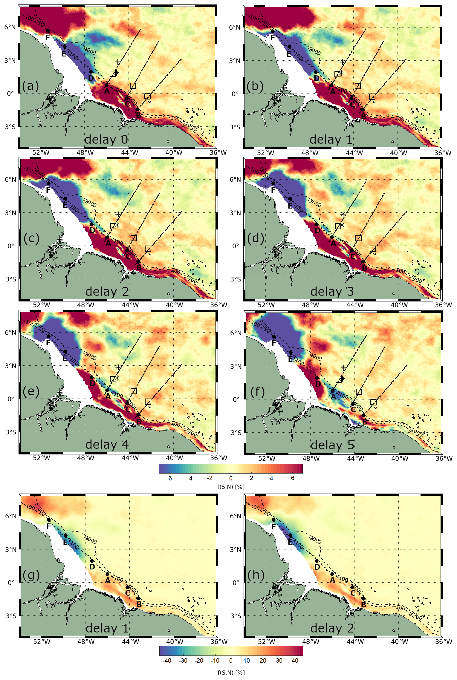
Figure 7 Spring-neap tidal cycle composites of CHL using daily Globcolour product, considering delays of (a–f)  0–5 d. Spring-neap tidal cycle composite map for delay of (g) 1 d and (h) 2 d, using a color bar for highlighting the shelf. Areas of high CHL fortnightly power are shown as black rectangles, IT generation points are displayed as black points, IT pathways are shown as black dashed lines according to Assene et al. (2024), and black stars represent the areas of high ISW occurrence according to de Macedo et al. (2023).

In the offshore region between IT generation points A and B, a positive spring–neap tidal cycle difference is observed, following a wave-like pattern in the horizontal structure of CHL. This wave pattern is most pronounced with a 1 d delay from the spring–neap tides, gradually diminishing in extent and coherence with longer delays. Referring to the spring–neap tidal cycle composites with a 1 d delay as a benchmark, Fig. 7b illustrates at least three peaks of positive CHL spring–neap tidal cycle difference. Figure A2a shows a close-up view highlighting the wave-like pattern in the CHL composite with a 1 d delay. The profiles along the IT pathways A, B, and C for spring–neap tidal cycle composites are shown in Fig. 8. Taking as reference the delay of 1 d, an average of 63 km separates the two first peaks and the second and third peaks are 83 km apart. The distances of the three peaks from IT generation points A, B, and C are detailed in Table 1. In Fig. 7, the black stars indicate areas with frequent ISW occurrences based on findings by de Macedo et al. (2023). The third peak of positive CHL difference along pathway A is flanked by the regions of high ISW occurrence.

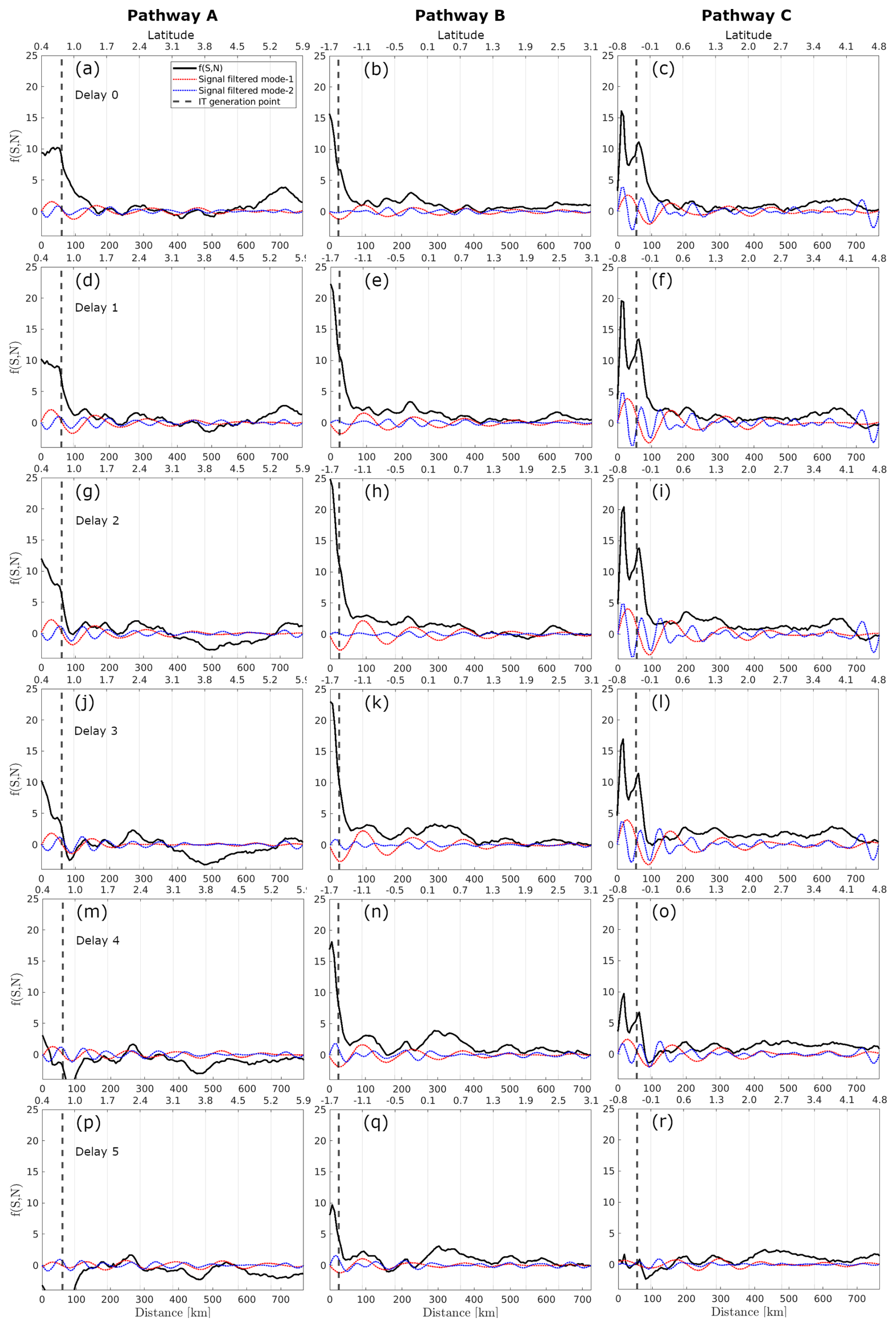
Figure 8 Profiles along the A, B, and C pathways (columns) of the spring–neap tidal cycle CHL composite using Globcolour, considering delays of 0–5 d. black and dashed red and blue lines represent, respectively, the original signal and the signal filtered for mode-1 (100–150 km) and mode-2 (50–100 km) wavelengths.

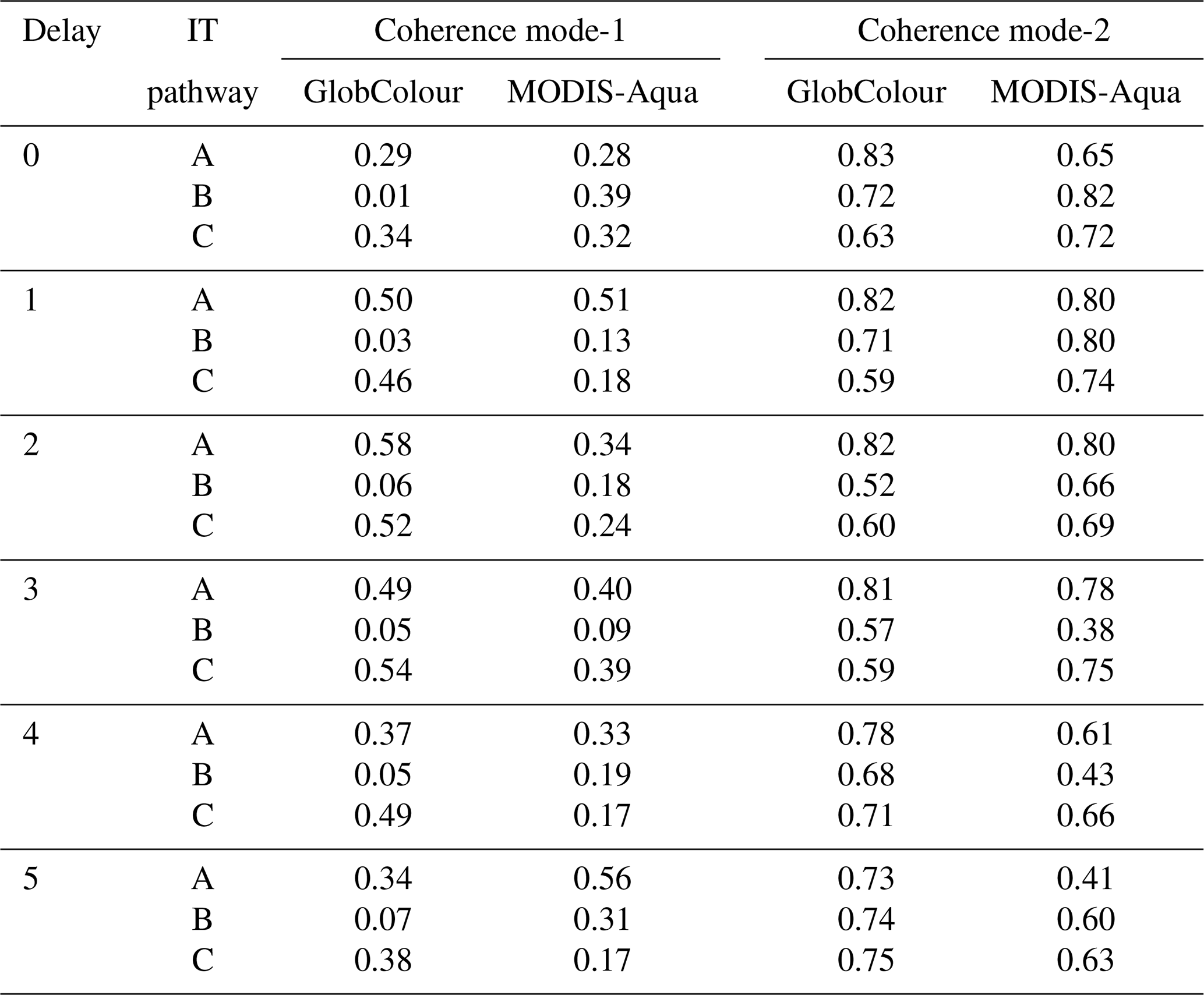
In Fig. 8, focusing on IT pathway A and a 1 d delay from spring–neap tides, the positions of the first and third peaks correspond closely to the peaks of positive CHL relative difference observed in illustrative cases I and II (see Fig. 5e and f). Additionally, the locations of the second peak of positive spring–neap tidal cycle CHL difference along IT pathways A and C, and the third peak along IT pathway B, correspond closely with areas of high Morlet wavelet power (indicated by gray dashed rectangles in Fig. 7b). The positive peaks of CHL differences during the spring–neap tidal cycle, with a 1 d delay, average around 2.1 % across all IT pathways. The modulation of spring–neap tidal cycle differences filtered for mode-1 and mode-2 IT wavelength diminishes further offshore after the initial 300–400 km. The mean spectral coherence between spring–neap tidal cycle signal and the band-pass filter component is higher for mode-2 than mode-1, considering all delays (see Table 2)

When considering the signal filtered for mode-1 wavelength, the modulations in the spring–neap tidal cycle composite map are less coherent along IT pathway B. However, the peaks of positive spring–neap tidal cycle CHL differences reach higher values along IT pathway B. This finding aligns with the Morlet wavelet analysis, which indicates higher fortnightly power along IT pathway B than other pathways. In contrast, lower values are observed along pathway A (see values in Table 1) compared to other IT pathways. Note that, when considering a profile outside the influence of ITs, the signal filtered for mode-1 and mode-2 IT wavelengths are very low (see Fig. A3).

Table 1 Distance (km) from the IT generation sites and maximum values of CHL difference associated with the three first beams along the IT pathways A, B, and C, for GlobColour (1 d of delay from the spring–neap tides) and MODIS-AQUA data (2 d of delay).

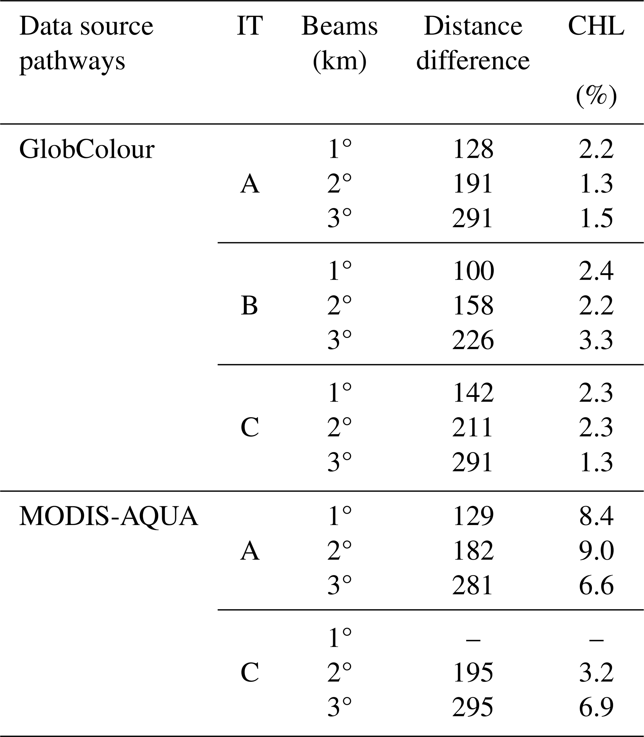
Table 2 Mean spectral coherence for modes 1 and 2 along IT pathways (A, B, C) for GlobColour and MODIS-Aqua dataset at different delays.

Because of the temporal averaging and interpolation methods involved in deriving CHL concentration from the GlobColour product, we also generated spring–neap tidal cycle composites using daily MODIS-Aqua imagery, as shown in Fig. 9. Due to the substantial cloud cover in our study area, these composites are noisier than the GlobColour ones. Nevertheless, both datasets reproduce similar spatial patterns, particularly on the shelf region, where a comparable dipole pattern is evident in MODIS-Aqua as in GlobColour composites. In the northwest part of the shelf, MODIS-Aqua composites show maximum negative CHL differences (approximately −84 %) occurring 2–3 d after spring–neap tides, whereas in the northeast region, maximum positive CHL anomalies of about 70 % are observed under similar timing. Overall, CHL differences between spring and neap tides tend to be higher in MODIS-Aqua compared to GlobColour composites.

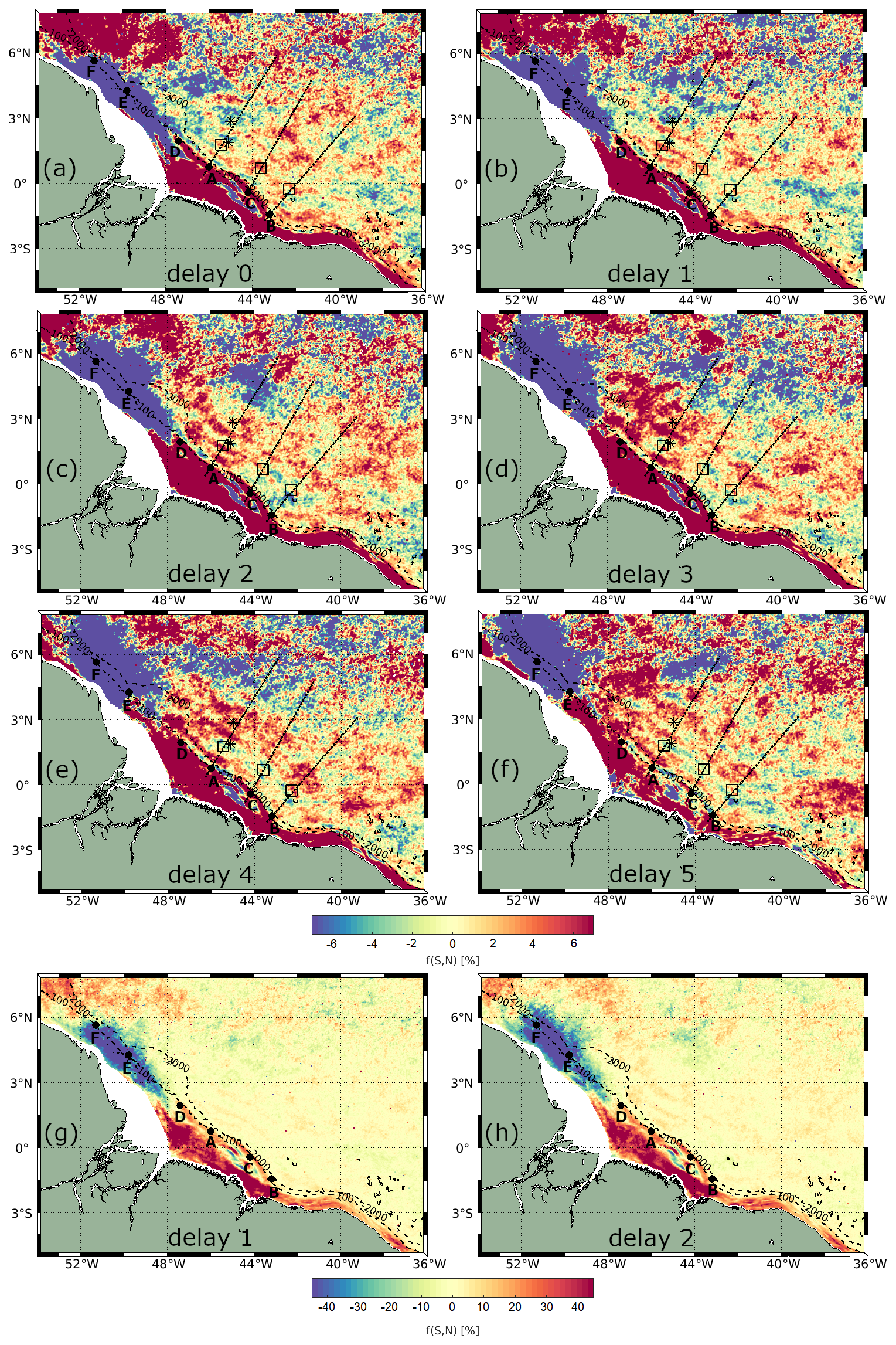
Figure 9 Spring-neap tidal cycle composites of CHL using daily MODIS-Aqua data, considering delays of (a–f) 0–5 d. Spring-neap tidal cycle composite map for delay of (g) 1 d and (h) 2 d, using a color bar for highlighting the shelf. Areas of high CHL fortnightly power are shown as black rectangles, IT generation points are displayed as black points, IT pathways are shown as black dashed lines according to Assene et al. (2024), and black stars represent the areas of high ISW occurrence according to de Macedo et al. (2023).

Offshore, a distinct wave pattern emerges with a 2 d delay, characterized by at least three peaks of positive CHL spring–neap tidal cycle differences along pathway A. A close-up view highlighting the wave-like pattern in the CHL composite, with 2 d delay is shown in Fig. A2b. A similar pattern is partially visible along pathway C, which exhibits two peaks of positive CHL spring–neap tidal cycle differences. Along pathway A, the third peak of positive CHL difference is in between regions of frequent ISW occurrence (de Macedo et al., 2023), aligning with the patterns observed in GlobColour composites. Figure 10 illustrates the CHL difference profiles along the IT pathways for MODIS-Aqua composites. For a 2 d delay, along pathways A and C, the CHL spring–neap tidal cycle difference peaks average around 6.8 %, more than double the signal detected in GlobColour composites. The wave-like structure begins to lose coherence after a 3 d delay from the spring–neap tides. The spatial distribution of the CHL concentration peaks closely aligns with the wave structures observed in GlobColour composites along IT pathways A and C (see Table 1). In contrast, no significant signal is detected along pathway B in the MODIS-Aqua composites. In both pathways A and C, the signal filtered for mode-2 IT wavelength is more coherent than the signal filtered for mode-1 (see Table 2).

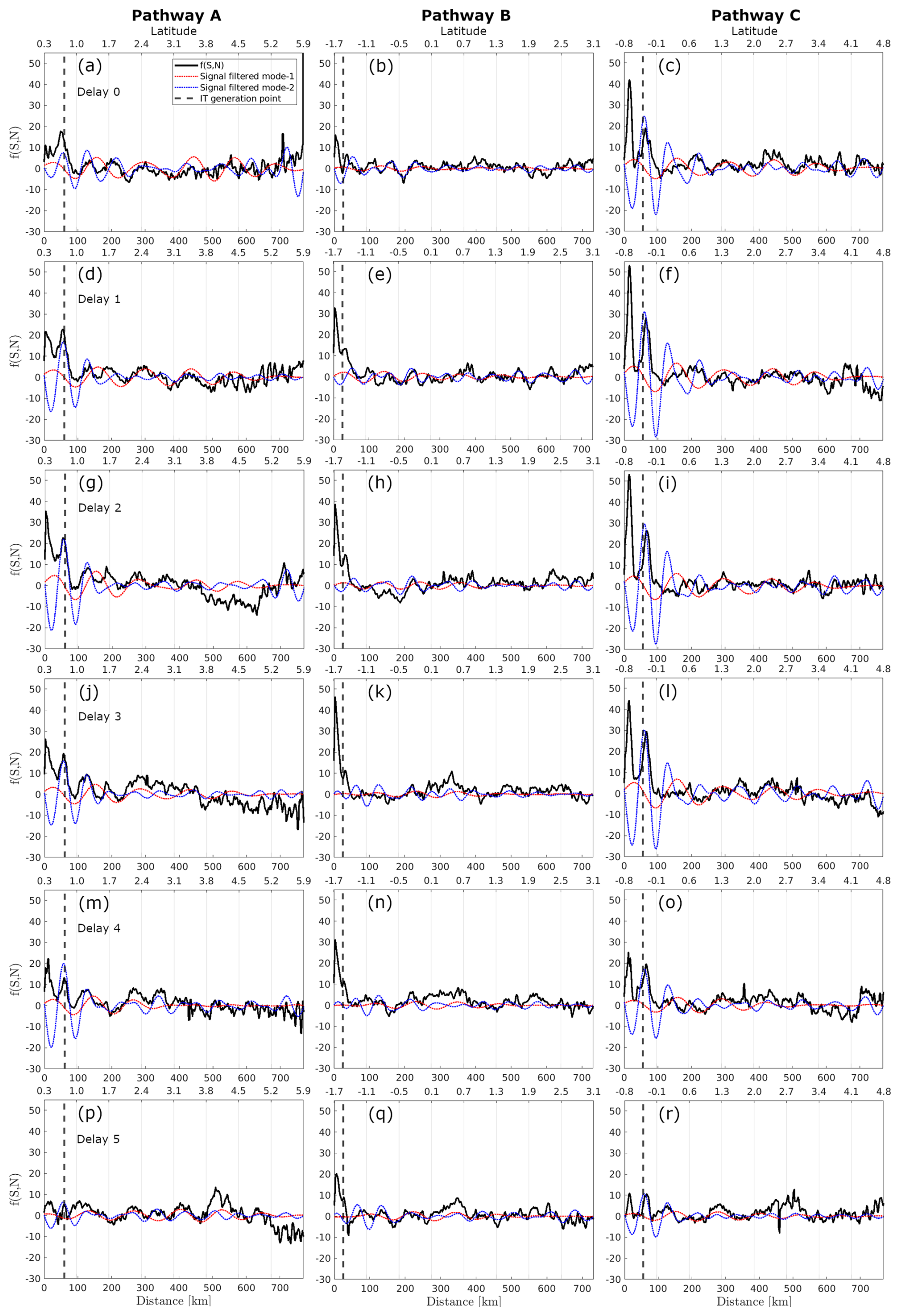
Figure 10 Profiles along the A, B, and C pathways (columns) of the spring–neap tidal cycle CHL composite using MODIS-Aqua, considering delays of 0–5 d. black and dashed red and blue lines represent, respectively, the original signal and the signal filtered for mode-1 (100–150 km) and mode-2 (50–100 km) wavelengths.

4 Discussion

4.1 IT illustrative cases

The offshore band of enhanced CHL in illustrative cases I and II (around 2.5° N, 45.5° W, see Figs. 3 and 4) likely corresponds to an IT crest, as two ISW signatures flank it. Similar bands of elevated CHL levels, flanked by ISW signatures, were observed by da Silva et al. (2002) and Muacho et al. (2014) in the Bay of Biscay. They attributed the enhanced CHL concentration to the uplifting of the DCM caused by the passage of internal tidal crests.

The CHL concentration bands associated with the IT in our illustrative cases are 7 % to 31 % higher than the 15 d average, aligning well with the findings of M'hamdi et al. (2025). Their study, based on data from a Slocum G2 glider equipped with an optical fluorescence sensor deployed off the Amazon shelf, reported that ITs increase total chlorophyll concentration by 14 % to 32 %.

4.2 Wavelet analysis

The findings indicate that the highest CHL and SST fortnightly mean Morlet wavelet power occurs on the shallow shelf, where barotropic tides dissipate through bottom friction (see Fig. 6c). Based on these surface measurements, we infer that this dissipation induces mixing, likely impacting water properties.

The fortnightly signal in SST is weaker than that observed in CHL and becomes even less pronounced offshore. Using two regional simulations (with and without tides), Assene Mvongo (2024) estimated sea temperature anomalies along IT pathway A and reported offshore surface anomalies of approximately −0.2 °C. The study also showed that ITs modulate upper ocean–atmosphere interactions by enhancing the net heat flux at the air–sea interface. This enhanced flux from the atmosphere to the ocean tends to damp the IT-induced SST cooling and contributes to restoring surface temperatures (Assene Mvongo, 2024). Such restoration could explain the weaker fortnightly signal in SST compared to CHL. Nevertheless, further studies are needed to understand these differences better.

4.3 Spring–neap tidal cycle composite

On the shelf, using 1 and 2 d delays as benchmarks for GlobColour and MODIS-Aqua CHL composites, respectively (see Figs. 7b and 9c), based on surface measurements, we infer that the northwestern region, influenced by the turbid Amazon River plume, may experience higher sediment resuspension and mixing during spring tides, which in turn may inhibit primary production due to light limitation. In shallow, permanently mixed areas of the northwest European shelf, tidal mixing and resuspension of suspended matter hinder primary production, as Kossack et al. (2023) noted. According to Nittrouer et al. (2021), near the Amazon River mouth, energetic spring tides resuspend muddy sediment in the water column, making fluid mud less dense and well-mixed but, during neap tides, the tides are less energetic and denser fluid mud consolidates on the seabed. Another possible explanation for the negative spring–neap tidal cycle CHL anomaly observed in this region is the influence of tidal variability on the Amazon River plume dynamics. During spring tides, strong vertical turbulence shifts the northeastward deflection of the plume waters further offshore. In contrast, during neap tides, the plume is deflected right upon entering the ocean remaining closer to the shore (Ruault et al., 2020). In neap tide reduced mixing results in a well-stratified river plume, limiting nutrient dispersion and leading to higher nutrient concentrations within the plume. Under these conditions, phytoplankton likely can access these nutrients, considering that the light availability is sufficient. In the northeastern shelf region, where lower turbid waters are present (non-plume waters), we can infer that the dissipation of barotropic tides likely promotes mixing, which may contribute to enhancing CHL concentrations. As Kossack et al. (2023) highlighted, tidal fronts in the northwest European shelf promote vertical mixing of nutrients, enhancing primary production, with approximately 16 % of annual mean primary production attributed to tidal forcing in these regions.

4.3.1 Tide-aliasing effect

Figure 11 illustrates the tidal amplitudes and phases observed in all images composing the MODIS-Aqua time series. Imagery acquired during spring tides approximately corresponds to low tide, while acquired during neap tides approximately corresponds to high tide. As noted by Valente and da Silva (2009), this tide-aliasing effect arises from the sun-synchronous orbit of the MODIS-Aqua satellite relative to local tidal patterns. Consequently, it is reasonable to hypothesize that the spring–neap tidal cycle composite signal may be influenced by the low-high tide chlorophyll dynamics. However, variations in chlorophyll (CHL) levels between low and high tides are likely minimal in deep waters and coastal regions. Blauw et al. (2012) observed a semi-diurnal pattern in the Southern North Sea, where surface phytoplankton concentrations decreased during high and low tides, coinciding with periods of weak tidal mixing. In contrast, chlorophyll levels increased during transitional tidal phases (flood and ebb), when current speeds and mixing intensity were stronger. In this study, flood and ebb data were excluded, suggesting that the tide-aliasing effect is unlikely to significantly impact our results. Furthermore, it is expected that 6-hour periodic variations in chlorophyll are more pronounced in coastal areas and considerably weaker in the open ocean. Nevertheless, to the best of our knowledge, we could not find any study that has specifically addressed chlorophyll variations between high and low tides in our study area. It is worth noting that satellite overpasses occur at approximately the same local time each day, which minimizes potential impacts on chlorophyll related to light-dependent processes. An additional robustness is that we compared spring–neap tidal cycle composites from GlobColour (an ensemble product derived from multiple sensors and therefore less prone to tidal aliasing) with those from MODIS-Aqua. Both products show very similar patterns, which strengthens our confidence that high-low tidal aliasing does not significantly bias our results.

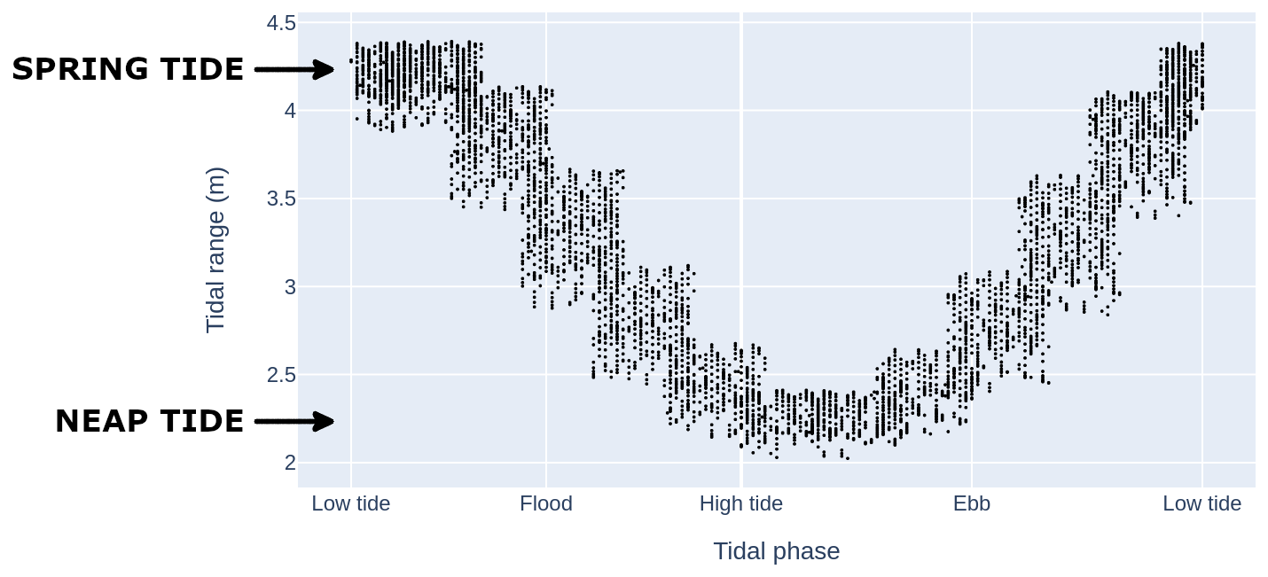
Figure 11 Illustration of the tidal range during the acquisition of all MODIS-Aqua scenes used in this study from 2005 to 2021.

4.3.2 Wave-like pattern observed in the spring–neap tidal cycle composites

The wave-like pattern observed in the spring–neap tidal cycle composites between IT generation sites A and C correlates well with the steric sea-surface height (SSSH) gradient along the northeast direction from the Hybrid Coordinate Ocean Model (HYCOM), as computed by Solano et al. (2023) (refer to their Fig. 9), where SSSH modulation is observed at approximately 65–70 km intervals in that region. Given the similarity between the horizontal structures of CHL variability in the spring–neap tidal cycle composite maps and SSSH patterns, it is likely that the propagation of semi-diurnal ITs and their possible resulting mixing are primarily responsible for the observed positive horizontal variability in CHL spring–neap tidal cycle composites (barotropic tides are considered negligible beyond the shallow shelf, as shown in Fig. 6c). Furthermore, the third peak of positive CHL difference along pathway A is flanked by the regions of high ISW occurrence (see Figs. 7 and 9), suggesting that the variation in CHL concentration in that area is likely linked to the passage of an IT crest.

The wave-like pattern could potentially arise from two different mechanisms, although these remain hypothetical: (1) tidal aliasing combined with the modulation of the DCM induced by the passage of interfacial ITs. Interfacial IT waves can lift the DCM above the light penetration depth, making it detectable by remote sensing instruments (da Silva et al., 2002; Muacho et al., 2014; Kim et al., 2018; M'hamdi et al., 2025). As for tidal aliasing, this would imply that MODIS-Aqua repeatedly observes IT crests in nearly the same location, given that both IT generation and the satellite orbit are synchronized with the M2 tidal constituent. However, this explanation remains speculative and requires further investigation, especially considering that two semidiurnal tidal cycles are merged and averaged in the 1 d GlobColour product. (2) Internal tide beams, which could potentially reduce subsurface light limitation for primary production and enhance nutrient fluxes that further stimulate biological activity (Althaus et al., 2003; Jacobsen et al., 2023; Kouogang et al., 2025). Additional research is needed to better understand the origin of the observed wave-like pattern.

Incoherent tides

It is reasonable to assume that the wave pattern in the composite maps is likely partially averaged out by interactions of the ITs with background circulation features, including eddies, currents, and stratification. These interactions generate incoherent IT patterns that shift locations throughout the year, likely diminishing the IT signal in CHL composites. For instance, CHL modulation in the illustrative cases we presented in Sect. 3.1 can be up to 30 % higher than the CHL 15 d average, i.e., much higher than the weaker signal in the CHL composites.

Different processes of influences

The wave patterns observed in CHL spring–neap tidal cycle composites from GlobColour and MODIS-Aqua exhibited modulations in signals filtered for both mode-1 and mode-2 internal tide (IT) wavelengths. This suggests that the patterns may arise from a combination of mode-1 and mode-2 ITs, and/or interference between these modes. The mean spectral coherence between spring–neap tidal cycle signal and the band-pass filter component is higher for mode-2 than mode-1, considering both GlobColour and MODIS-Aqua data (see Table 2). For example, when considering a 1 d delay, the spectral coherence is approximately 0.50 for mode-1 and 0.81 for mode-2, for both GlobColour and MODIS-Aqua datasets. It can indicate that CHL is more sensitive to the physical processes typically associated with higher internal-tide modes. As discussed in previous studies, the redistribution of low-mode energy flux to higher modes through interactions with the background circulation provides an important mechanism for driving mixing away from internal-tide generation sites; scattering to higher modes allows for greater vertical propagation and energy dissipation (Kerry et al., 2014; Dunphy and Lamb, 2014; Savva and Vanneste, 2018; Tuerena et al., 2019; Lahaye et al., 2020; Li and Xie, 2023). However, further research is required for a more comprehensive explanation.

Results suggest that the spring–neap tidal cycle composites from the GlobColour product are more effective for capturing spatial patterns of CHL modulation by ITs, thanks to their lower proportion of missing data. While some CHL modulation patterns may be lost in the noisier MODIS-Aqua composites, likely due to high cloud coverage, these composites may provide better estimates of the potential amplitude of CHL concentration variations.

Phytoplankton response time

Our results showed that the lag between the tidal potential and the peak chlorophyll variability, possible indicative of maximum mixing, ranges from 1 to 3 d after the spring–neap tides. This variation depends on the CHL data source used to calculate the spring–neap tidal cycle composites. The differences could arise from the use of merged versus non-merged data, as well as variations associated with different models, including atmospheric corrections and chlorophyll retrieval algorithms. Assene Mvongo (2024) showed that maximum temperature variability associated with tidal mixing occurs on average 2–3 d after spring tides in the BEM. Similarly, Shi et al. (2011) found that maximum turbidity and suspended matter occur with a 2 d delay from spring tide in the Yellow Sea. Another delayed impact of IT mixing is the increased nutrient availability in the euphotic zone, which can lead to an increase in biomass after a few days. The exact time lag between IT mixing and productivity depends on light availability, nutrient supply induced by the tides and the phytoplankton community and its associated growth rates (Wang et al., 2011; M'hamdi et al., 2025).

5 Summary and conclusions

In this study, we analyzed remotely sensed chlorophyll a (CHL) concentration data to provide analysis of how tides influence the surface spatial variability of CHL concentration in the Brazilian Equatorial Margin. For the first time, our findings reveal the presence of the internal tide (IT) signal in CHL data in the region, identified through an extensive time series analysis.

The findings indicate that the highest CHL fortnightly mean Morlet wavelet power and variability in the spring–neap tide composites occur on the shallow shelf. In the northwestern shelf, the CHL concentration is higher during neap tides (i.e., negative spring–neap tide CHL anomaly; −50 % in GlobColour and −84 % in MODIS-Aqua). In the northeastern part of the shelf, where ocean waters are less turbid, the chlorophyll concentration is higher during neap tides (30 % in GlobColour and 70 % in MODIS-Aqua).

Surface signatures in CHL concentration are shown to be consistent with the influence of ITs while they propagate offshore. Two illustrative cases based on MODIS-Aqua imagery reveal along IT pathway A bands of CHL concentration up to 30 % higher than the 15 d chlorophyll average. We infer that these bands are likely associated with the passage of IT crests, as the outermost band is flanked by regions with a high occurrence of ISWs, as reported by de Macedo et al. (2023). Moreover, the IT pathways A, B, and C show a distinct wave pattern in the horizontal structure of the GlobColour spring–neap tidal cycle CHL compositions, marked by a positive spring–neap tidal cycle anomaly. The spatial positions of the positive spring–neap tidal cycle CHL anomalies align well with areas of high CHL fortnightly Wavelet power. The wave pattern appears clearer and more coherent in the Globcolour composites than those from MODIS-Aqua. In the Globcolour composites, three beams of CHL-positive anomalies are visible along the three IT pathways, reaching up to approximately 3.3 %. Similarly, the MODIS-Aqua composites display three beams of CHL-positive anomalies along IT pathway A and two beams along IT C, with the beam locations aligning well with those in the Globcolour composites but with higher CHL anomalies reaching up to 9.0 %. No significant signal is observed along pathways B, for MODIS-Aqua data. The beam signal in the GlobColour and MODIS-Aqua composites is attenuated after 300–400 km. Spring-neap tidal cycle composites derived from the merged GlobColour product appear to more effectively capture the spatial patterns of CHL modulated by ITs, possibly due to their lower proportion of missing data compared to MODIS-Aqua. Conversely, MODIS-Aqua composites may better represent the relative amplitude of CHL concentration variations. The differences between GlobColour and MODIS-Aqua composites may be related to the use of merged versus single-sensor products and to methodological differences, including atmospheric correction procedures and chlorophyll retrieval algorithms

Wave patterns in CHL spring–neap tidal cycle composites from GlobColour and MODIS-Aqua suggest contributions from mode-1 and mode-2 ITs, with mode-2 components having higher spectral coherence with the original signal. However, further research is needed for clarity. Results indicate a lag of 1–3 d between spring–neap tides and peak chlorophyll variability, indicative of maximum mixing. ITs exhibit a more distinct fortnightly variability on surface CHL than on SST.

ITs might be responsible for an increase in productivity offshore of the Amazon River, as in other areas of the global ocean. However, these effects still need to be better quantified, and the associated processes understood to predict their potential changes due to climate change. In the future, a coupled physical–biogeochemical model could be employed to quantify the productivity associated with ITs off the Amazon shelf, helping to disentangle the various processes that may explain the CHL signal and to estimate nutrient fluxes.

Appendix A

Figure A1 shows the sea level anomaly (SLA) and geostrophic currents derived from the Global Ocean Gridded L4 Sea Surface Heights and Derived Variables Reprocessed (1993–ongoing) product (https://doi.org/10.48670/moi-00148, Copernicus Marine Service, 2023b), with a spatial resolution of 0.125°×0.125°, available through the Copernicus Marine Service (https://data.marine.copernicus.eu/, last access: 15 September 2025). The gridded SLA fields are computed relative to a 20-year (1993–2012) mean and estimated via optimal interpolation by merging along-track L3 measurements from multiple altimeter missions. Figure A2 presents a zoom that highlights the wavelike pattern in the horizontal structure of the spring–neap tidal cycle CHL composites, with a 1 d delay for the GlobColour product and a 2 d delay for the MODIS-Aqua images. Figure A3 shows the spring–neap tide CHL composite signal filtered for mode-1 and mode-2 IT wavelengths along a profile located outside the region influenced by ITs. As expected, the filtered signal in this area is weak.

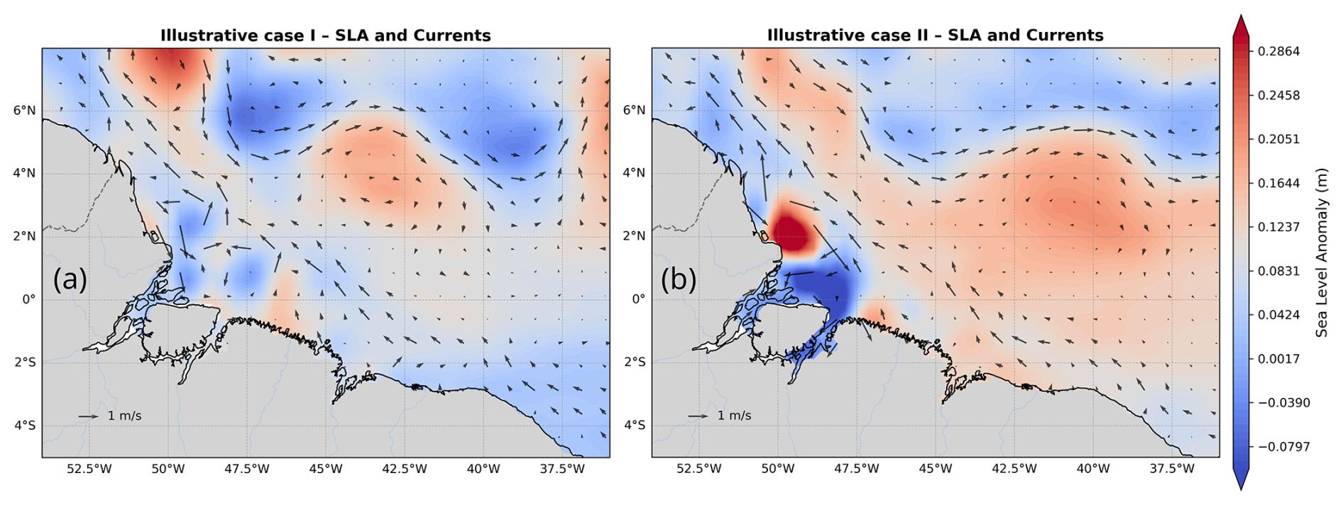
Figure A1 SLA (color shading) and surface geostrophic currents (arrows) for the two illustrative periods: (a) case I and (b) case II.

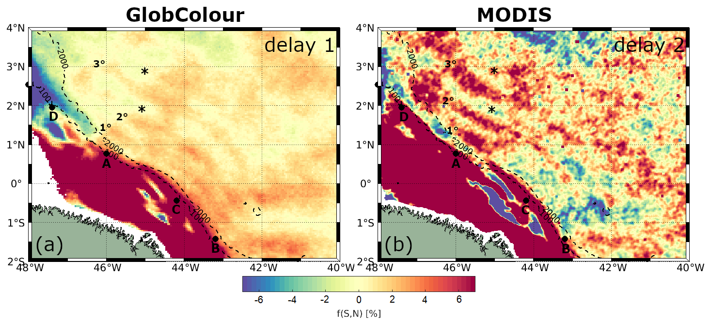
Figure A2 Zoomed in version of Figs. 7 and 9 highlighting the wave-like pattern in the horizontal structure of spring–neap tidal cycle CHL composites for (a) GlobColour, with a 1 d delay, and (b) MODIS-Aqua, with a 2 d delay. IT generation points, as identified by Assene et al. (2024), are indicated by black dots, while areas of high ISW occurrence, based on de Macedo et al. (2023), are marked with black stars. The numbered labels denote the first, second, and third positive peaks in the CHL composites.

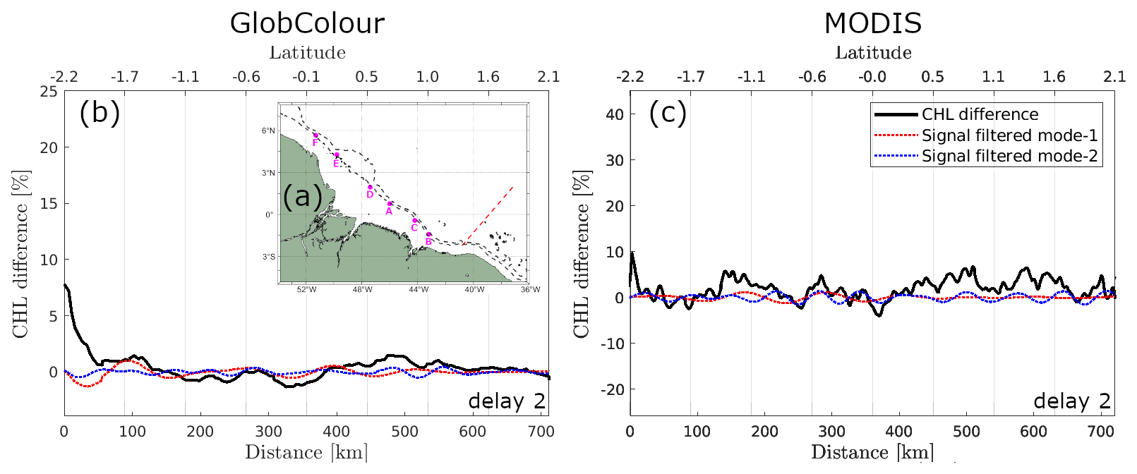
Figure A3 (a) Map of the study area highlighting the selected transect (red dotted line), which serves as a reference for a region unaffected by IT influence. Panel (b) shows the CHL composite profiles along this reference transect using GlobColour and (c) MODIS-Aqua. The black line represents the original signal, while the dashed red and blue lines correspond to signals filtered for mode-1 (100–150 km) and mode-2 (50–100 km) wavelengths.