Internal solitary waves refraction and diffraction from interaction with eddies off the Amazon Shelf from SWOT

Off the Amazon shelf, internal solitary waves (ISWs) generated by internal tides interact with mesoscale eddies, leading to significant modifications in their propagation and structure. For the first time, these interactions are directly observed from repeated high-resolution satellite measurements, notably those provided by the newly launched SWOT (Surface Water and Ocean Topography) mission.

The study investigates ISWs detection and the modifications in ISW's characteristics resulting from interactions with eddies across three contrasting scenarios: ISW propagation in the absence of mesoscale eddies, ISW refraction by a cyclonic eddy, and ISW diffraction by an anticyclonic eddy. ISW crests are extracted using a band-pass filtering approach, enabling precise tracking of essential geometric and dynamical features, including propagation direction, crest-to-crest spacing, and wavefront shape. Prior to any interaction with eddies, three mode-1 ISW packets propagate in a steady and coherent manner, exhibiting planar wavefronts and consistent direction, with Absolute Dynamic Topography (ADT) amplitudes ranging from 8 to 14 cm.

The results highlight the diversity of ISW responses depending on eddy conditions. In the absence of eddies, interaction with a seamount induces energy transfer from mode-1 to mode-3 ISWswaves (13 crests detected), while propagation direction is maintained and the ADT signature weakens to below 8 cm. In the presence of a cyclonic eddy above the seamount, ISW trajectories are refracted westward by roughly 50 degrees (7 crests detected), with increased wavecrest curvature and intensification of mode-3 generation, while ADT amplitudes decrease below 6 cm. Conversely, near the western boundary of an anticyclonic eddy, ISWs split into two distinct pathways: a western branch is refracted with flatter wavefronts, reduced crest spacing, and ADT amplitudes below 0.2 cm (9 crests detected), while an eastern branch follows the eddy's edge, displaying enhanced curvature, recognizable surface signatures of wave packets, and ADT values exceeding 9 cm (6 crests detected).

Together, these findings demonstrate the ability of SWOT-based monitoring to capture the complexity of ISW dynamics and provide new insight into their nonlinear response to interactions with mesoscale and submesoscale oceanic structures.

1 Introduction

Internal tides (ITs) are internal waves generated by the interaction of barotropic tidal currents with bathymetric features such as continental slopes, ridges, or seamounts, in a stratified ocean. These baroclinic waves propagate in the ocean interior and can span hundreds of kilometers. When ITs propagate into regions of variable stratification or shallow topography, or when they encounter other waves or dynamical currents, nonlinear processes can cause them to steepen and disintegrate into trains of short, high-amplitude internal solitary waves, ISWs (Jackson et al., 2012; Alford et al., 2015). ISWs often appear as wave packets and can propagate over long distances. The spacing between packets reflects the tidal forcing, ranging from over a hundred kilometers for mode-1 ITs to only a few kilometers for higher-order modes (de Macedo et al., 2023; Tchilibou et al., 2025; Le Mercier et al., 2012). Typically interfacial, ISWs travel horizontally along the seasonal or permanent pycnocline (Gerkema, 2001; Grisouard and Staquet, 2011). The ISWs trajectories and properties are modulated by local environmental factors – including background currents, mesoscale eddies, stratification, and bathymetric features – on timescales ranging from daily to interannual (Müller et al., 2012; Nash et al., 2012; Vlasenko et al., 2012; Magalhães et al., 2016; Liu and D'Sa, 2019; Tchilibou et al., 2022; Barbot et al., 2021).

ISWs are associated with strong vertical velocities and intense mixing, which impact the redistribution of physical and biogeochemical properties in the upper ocean (Beninger et al., 2024; Assene et al., 2024; de Macedo et al., 2025; M'hamdi et al., 2025; Capuano et al., 2025). They contribute to energy cascades, air–sea exchanges, and ecosystem structuring (Sandstrom and Elliott, 1984; Huthnance, 1995; Munk and Wunsch, 1998; Muacho et al., 2013; Solano et al., 2023; Assene et al., 2024). ISWs also pose risks to offshore operations by destabilizing underwater structures and threatening navigation safety – a concern that is particularly relevant along the Brazilian Equatorial Margin, where a rapid expansion of oil and gas exploration is expected in the near future (Bole et al., 1994; Hyder et al., 2005; He et al., 2024). A better understanding of ISW–eddy interactions is thus essential for ocean energy budgets and hazard assessment, as eddies can transfer energy to higher modes and generate wave interference (Dunphy and Lamb, 2014; Ponte and Klein, 2015; Dunphy et al., 2017).

The oceanic region facing the Amazon mouth constitutes a laboratory of experiment for studying IT and ISW interaction with dynamical mesoscale as the region is well known for IT and ISW generation and the mesoscale activity induced by high dynamical currents (Fig. 1a and b).

First, the region exhibits more than six IT generation sites along the Amazon Shelf break (Fig. 1b), from A to F (Magalhães et al., 2016; Tchilibou et al., 2022), with the most energetics A and D that converge and B (Fig. 1b). As they propagate, IT energy fluxes from A and D interact together and with the background environment, become unstable, and potentially disintegrate into ISWs packet that have been observed propagating several hundred kilometers from the shelf break (Magalhães et al., 2016; de Macedo et al., 2023, Fig. 1b). These waves probably cause intensified hot spots of mixing at more than 400 km from the shelf break (Kouogang et al. 2025a).

Second, off the Amazon, the region is influenced by the passage of an intense western boundary current, the North Brazil Current (NBC), which flows along the Brazilian coast (Fig. 1a). This current forms a retroflection that feeds the North Equatorial Countercurrent (NECC) and generates mesoscale activity with seasonal variability (e.g. Aguedjou et al., 2019). Indeed, from March to July (MAMJJ), the pycnocline is shallow and the NBC is weak, while the river discharge of the Amazon River is high. Consequently, the internal tide flux remains relatively stable and coherent (the phase-locked, relatively stable part of the IT) . From August to December (ASOND), the pycnocline deepens, the river discharge decreases, and NBC intensifies (Silva et al., 2005; Aguedjou et al., 2019; Tchilibou et al., 2022), which forms NECC. Instabilities in these currents generate a series of cyclonic and anticyclonic eddies (Garzoli et al., 2004). These structures significantly modify ISW propagation, trajectory, speed, amplitude, geometry, interpacket distance, and increase the incoherent, component of the internal tide (the non-phase-locked, time-varying part of IT; Bendinger et al., 2025; Dunphy and Lamb, 2014; Ponte and Klein, 2015; Dunphy et al., 2017; Wang and Legg, 2023; Xie et al., 2015; Xu et al., 2020; Huang et al., 2024).

Observational evidence of ISWs dynamics on sea surface height has long been limited by one-dimensional nadir altimetric measurements and by the low effective resolution of gridded multimissions altimetric products, which are capable of detecting only oceanic features larger than several hundred of kilometers, especially close to the equator (Chelton et al., 2007; Ballarotta et al., 2019). The SWOT mission offers, for the first time, real-time, repeated and two-dimensional observations of the ocean surface of 2 km resolution with an effective resolution of approximately 7–10 km (low rate product) (Morrow et al., 2019). SWOT can measure both sea surface height (SSH) with its Ka-band radar interferometer (KaRIn) and surface roughness (sigma0) using its SAR radar. The combination of these datasets represents a significant advancement for the precise detection and tracking of ISWs (Fu et al., 2024; Morrow et al., 2019; Cheshm et al., 2025; Qui et al., 2024; Zhang and Li, 2024). But this advance comes with new challenges. Currently, SWOT (Surface Water and Ocean Topography) data are corrected only for the stationary internal tide component using the High Resolution Empirical Tide (HRET) model (Zaron, 2019), and therefore still contain substantial nonstationary and ageostrophic signals – including ISWs. These waves partly develop at wavelengths comparable to submesoscale structures such as fronts and filaments. A key challenge is to extract the ISW signal to study each process separately for modeling purposes and to accurately estimate geostrophic currents from SWOT measurements. Therefore, detecting ISWs and understanding their interaction mechanisms constitute both technical and scientific challenges due to their multiscale complexity and nonlinearity. In this study, we combine SWOT data, optical images acquired under sun glint conditions and daily MIOST (Multiscale Inversion of Ocean Surface Topography) maps to explore the impact of eddies on ISW properties. Specifically, we examine changes in distance between crests, mode shifts, propagation directions, and wavecrest curvatures. Three cases are analyzed: (1) a reference case involving ISW propagation in the absence of eddies interaction, (2) interaction with a cyclonic eddy and (3) interaction with an anticyclonic eddy. The paper is organized as follows. The satellites data are introduced in Sect. 2. In Sect. 3, we present eddies and ISWs detection methods. Section 4 provides our résults. Next, Sect. 5 presents discussion of the obtained results. Finally, a conclusion is provided in Sect. 6.

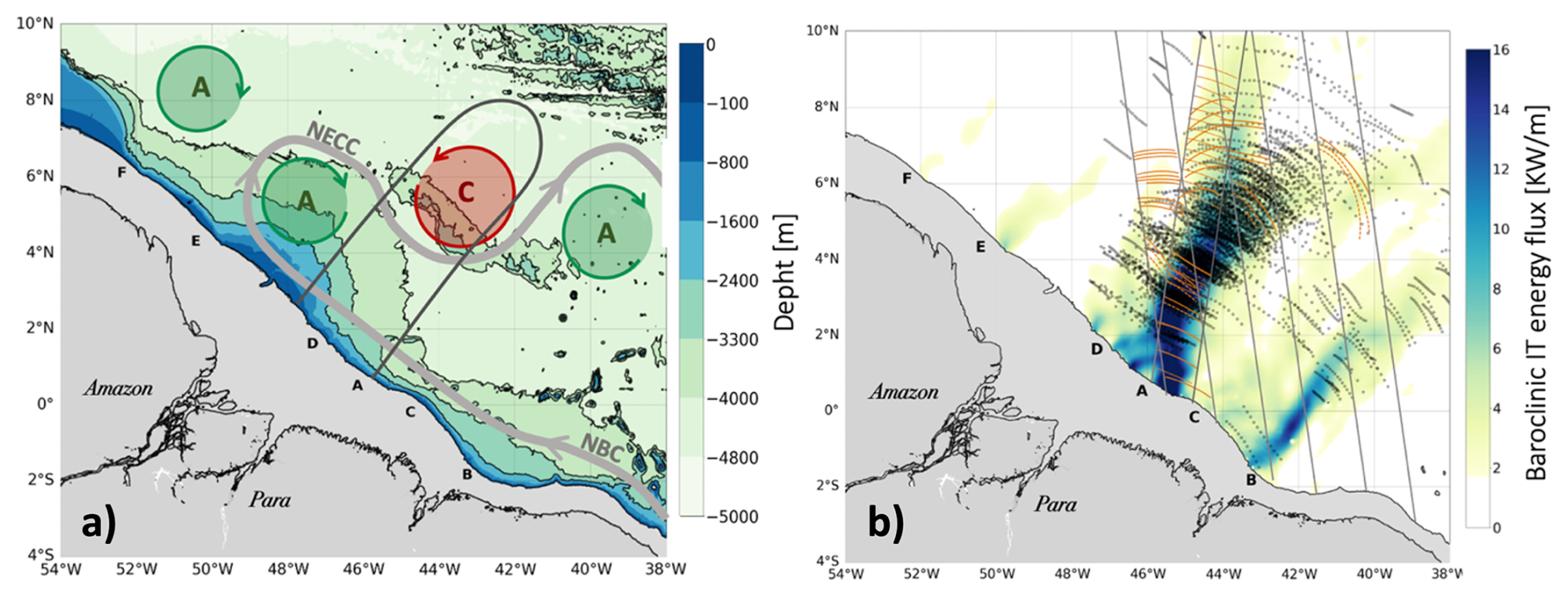
Figure 1 (a) Bathymetry of Amazon shelf from 0 to −5000 m. IT generation sites labeled A to F along the shelf break. Black solid contours delineate a typical area where ISWs propagation is observed from sites A and D. The NBC and NECC are highlighted with thick grey arrows. Cyclonic eddies (CE) and anticyclonic eddies (AE) are marked respectively by red and green circles. Seamounts are delineated by 4000 and 3300 m isobaths. Black solid contours delineate a typical area where ISWs propagation is observed from sites A and D. (b) The color map shows the 25-h mean depth-integrated baroclinic internal tide energy flux from the NEMO model from September 2015 (Assene et al., 2024), radiating from IT generation sites labeled A to F along the shelf break. ISW surface signatures (black dotted lines) detected in MODIS/TERRA satellite imagery from de Macedo et al. (2023) superposed with ISWs surface signature (orange line) detect in this paper on SWOT swath (grey lines).

2 Satellites data

Four complementary satellite datasets are used in the study, giving information on the location of real-time mesoscale structures. These includes the absolute dynamic topography (ADT) and ocean surface roughness from the new SWOT L3 KaRIn wide-swaths measurements, ADT maps from L4 multimission gridded product and optical data acquired by MODIS AQUA and NOAA-020 satellite. They are described in the following sections.

2.1 L4 MIOST DT experimental

ADT maps are used to investigate the oceanic dynamics off the Amazon shelf and to detect mesoscale eddies. The experimental daily MIOST maps are based on a multiscale, multivariate mapping of along-track altimetric observations from several satellites, including SWOT (KaRIn and nadir), SARAL/AltiKa, CryoSat-2, HaiYang-2B, Jason-3, Copernicus Sentinel-3A & 3B, and Sentinel-6A. These products are processed by SSALTO (Multimission ground segment for altimetry orbitography and precise localization)/DUACS (Data Unification and Altimeter Combination System) (Taburet et al., 2019) and distributed by AVISO with support from CNES (Centre national d'étude spatiales). The MIOST methodology (Ubelmann et al., 2021, 2022) enables improved reconstruction of ocean surface variability, particularly in delayed-time (DT) mode. This mode provides accurate mapping of mesoscale structures and reduces mapping error by more than half compared to near-real-time (NRT) products. MIOST reaches a spatial resolution of 0.125° × 0.125° (Ubelmann et al., 2021; Ballarotta et al., 2025). Off the Amazon shelf, the mapped wavelengths reach approximately 250–300 km, corresponding to processes with radius of about 70–90 km. The spatial resolution of MIOST maps is too low to resolve submesoscale processes, such as ISWs.

2.2 SWOT L3 product

To overcome these constraints, wide-swath radar interferometry solutions were developed and deployed with the SWOT mission. The Ka-band Radar Interferometer (KaRIn), the central instrument of SWOT, is a Ka-band radar interferometer equipped with two SAR antennas positioned on either side of the satellite. This setup enables two-dimensional (2D) altimetric measurements across two lateral swaths, each approximately 50 km wide, providing a total coverage of about 120 km across the track. KaRIn allows the resolution of ocean surface features at spatial scales around 15 km in wavelength (Morrow et al., 2019), about ten times finer than traditional gridded altimetry products. SWOT thus offers, for the first time, a snapshot of ISWs signatures in sea surface height (SSH), marking a significant advance in the study of their dynamics (Archer et al., 2025; Cheshm Siyahi et al., 2025). The orientation of the 21-d repeat cycle ascending passes is particularly well suited for observing tidal flows over the continental slope of the Amazon. The swaths are nearly perpendicular to the coastline and align with the typical ISW propagation direction (Fig. 1b). We use the SWOT Level-3 SSH Expert product v2.0.1 derived from the Level-2 SWOT KaRIn low rate ocean data products (L2_LR_SSH), on a 2 km spatial grid spacing. In order to obtain the total internal tide signal we sum the height of the sea surface anomaly unfiltered measured by KaRIn (ssha_karin_unfiltered), with all corrections and calibration applied and the coherent tidal correction from HRET (ssha_internal_tide) (Dibarboure et al., 2025). Then, the absolute dynamic topography (ADT_swot) is reconstructed by adding the mean dynamic topography (mdt_karin) (Jousset et al., 2025). In order to highlight high-frequency signals containing ISWs signatures, the MIOST ADT interpolated to SWOT resolution (adt_miost) is subtracted. Therefore, ADT_swot contains all the high-resolution signal not resolved by the corrections applied to the KaRIn data,as well as the part of the signal not resolved by the MIOST mapping method, including sub-mésoscale eddies, fronts, filaments, ISWs, internal gravity waves, wind waves.

$$\begin{array}{rl}\mathrm{ADT}\mathrm{\_}\mathrm{swot}& =\mathrm{ssha}\mathrm{\_}\mathrm{karin}\mathrm{\_}\mathrm{unfiltered}+\mathrm{ssha}\mathrm{\_}\mathrm{internal}\mathrm{\_}\mathrm{tide}\\ & +\mathrm{mdt}\mathrm{\_}\mathrm{karin}-\mathrm{adt}\mathrm{\_}\mathrm{miost}\end{array}$$

Another key measurement for observing ISWs is the surface roughness variation captured by the SAR radar backscatter. Joint analysis of SAR images (sigma0) and SWOT ADT enables the distinction between true soliton signals and other mesoscale or submesoscale structures. Thus, observing roughness contrasts facilitates the detection of soliton features.

2.3 MODIS AQUA and NOAA-020

To complement the limited spatial coverage of the SWOT dataset, which is limited to the swath width (∼120 km), we use one optical data for each case captured by different satellites. For no eddy case interaction (NE) and cyclonic eddy interaction case (CE), we used images captured by the MODIS (Moderate Resolution Imaging Spectroradiometer) instruments onboard the Aqua satellites, respectively (Level 1B MODIS/TERRA, https://doi.org/10.5067/MODIS/MYD021KM.061, MODIS Characterization Support Team, 2017). MODIS Level-1B dataset are accessible through NASA's Earth Science Data System (ESDS) (de Macedo et al., 2023). The measurements are acquired on band 6, centered at 1640 nm, with a spatial resolution of 500 m. For the anticyclonic eddy interaction case (AE), we utilized VIIRS Level 1-B calibrated radiance product (Visible Infrared Imaging Radiometer Suite) data acquired on bord the NOAA-20 satellite (https://doi.org/10.5067/VIIRS/VJ102MOD.021, VIIRS Calibration Support Team, 2021), which captures images at 750 m spatial resolution. Unlike the MODIS Level-1B product, which covers a 5-min time span, the VIIRS Level-1B calibrated radiance product has a nominal temporal duration of 6 min. These datasets highlight variations in ocean surface roughness. Under sunglint conditions, where solar reflections enhance contrasts, optical images reveal the signatures of solitons at the water surface. However, the number of usable observations is significantly limited by cloud cover, as well as the location and angle of solar reflection (de Macedo et al., 2023).

3 Methods

3.1 Eddy Detection Method

Mesoscale eddies were detected from ADT fields, as recommanded by Peliasco et al. (2022), derived from MIOST Level 4 products. To remove large-scale structures, we first applied a two-dimensional Lanczos filter to the ADT, with a cutoff wavelength of 1000 km in both latitude and longitude. This filtering highlighted mesoscale processes with a clear sea surface signature. Eddy detection was performed using the py-eddy-tracker algorithm (https://zenodo.org/records/7197432, last access: 5 November 2024; Delepoulle et al., 2022), based on the methods of Mason et al. (2014), Chelton et al. (2011), Kurian et al. (2011), and Penven et al. (2005).

The approach was based on the principle that, in a geostrophic regime, closed contours of SSH anomalies approximately followed streamlines. Eddy centers were identified as local extrema of ADT – maxima for anticyclonic eddies and minima for cyclonic eddies. Eddy edges were defined as the outermost closed ADT contours corresponding to the location of maximum geostrophic velocity, i.e., where the SSH gradient was strongest (Chaigneau et al., 2008).

The algorithm identifies closed ADT contours outward from the center in 1 mm increments. A contour was considered valid if it enclosed at least 90 connected grid points, corresponding to an effective radius of ∼60 km, based on the MIOST effective resolution. An amplitude threshold of 2 cm was applied to ensure the significance of detected structures and prevent excessive detections close to the coastline. Additionally, a shape criterion was used to exclude highly deformed structures that would inhibit coherent rotation. Contours with a shape error exceeding 50 % were discarded (Kurian et al., 2011; Mason et al., 2014).

3.2 ISW Detection

3.2.1 Spectral Analysis

Each SWOT track was subdivided into several windows located before and after the interaction zone between ISWs and the targeted eddy (Table 1). At first, for each window, the mean along-track wavelength spectrum was computed from ADT_swot signal to identify dominant wavelengths (Fig. 2a, black spectrum). In this region, ISWs come from the IT disintegration so we consider that distance between ISW packets correspond to typical wavelengths of IT-modes (Magalhaes et al., 2022; de Macedo et al., 2023; Tchilibou et al., 2022). Based on this, in second step, the dominant wavelengths of the spectrum (Fig. 2a, black spectrum) were isolated using a band-pass filter (Fig. 2a, blue spectrum), based on ranges corresponding to typical IT-modes: mode 1 (180–100 km), mode 2 (100–60 km), and mode 3 (60–30 km) (de Macedo et al., 2023; Tchilibou et al., 2022). The filter was constructed in the frequency domain by applying a Fast Fourier Transform (FFT), retaining only spectral components corresponding to the targeted wavelengths (Fig. 2a, blue spectrum). The filtered ADT_swot signal (Fig. 2b, blue line, bottom panel) was then reconstructed via inverse FFT. In the third step, local positive maxima in the filtered signal (Fig. 2b, blue line, bottom panel) were extracted (Fig. 2b, black crosses on blue line, bottom panel). Finally, each extracted pixels was mapped back on raw ADT_swot (Fig. 2b, black crosses on grey line bottom panel). This is done for all along track pixels of ADT_swot (Fig. 2b, black crosses on ADT swot swath, top panel). We coupled sigma 0 measurements for verify that the detected crests correspond to ISWs. Note that we tested different window sizes, which are presented in the Appendix. We specifically verified that windows smaller than 500 km provide the best correlations between the filtered signal (i.e., the detected ISWs) and the raw signal. In this study, we chose the largest possible window size to minimizing edge effects while avoiding the inclusion of additional submesoscale processes.

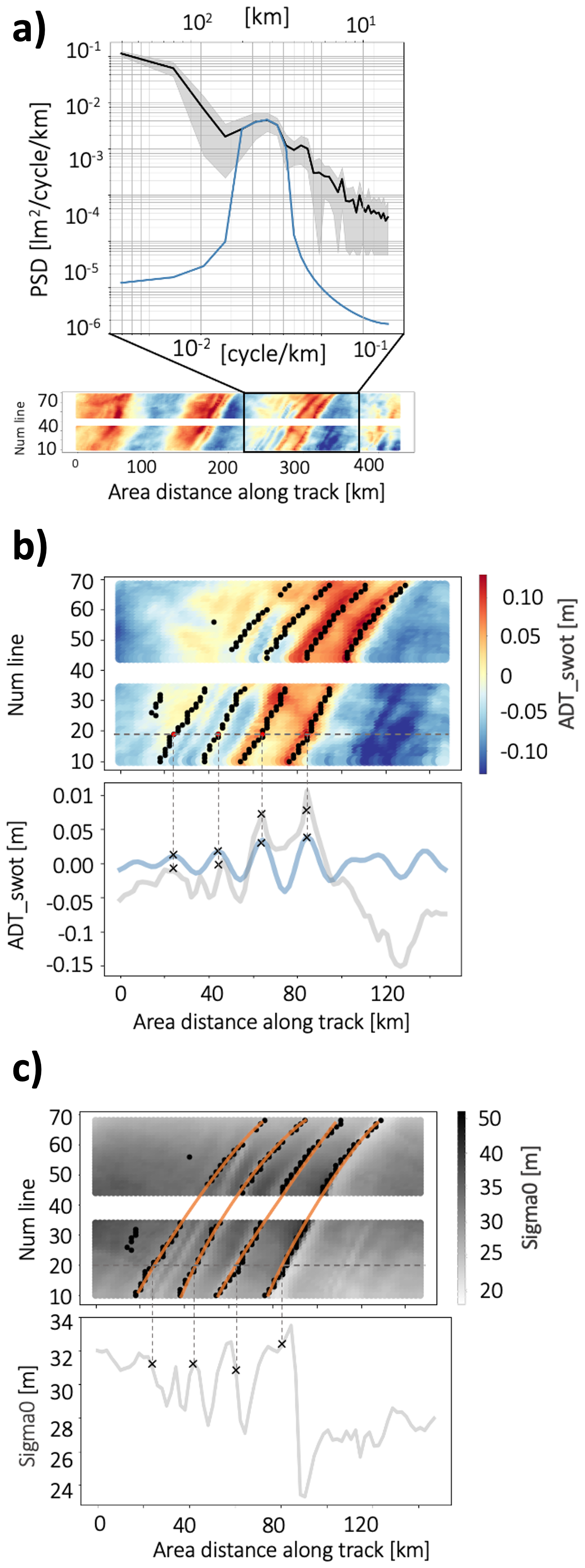
Figure 2 Method for one ISW packet detection. (a) Black line is mean along-track power spectrum density of ADT_swot signal with standard deviation envelope in gray and blue line is mean along-track power spectrum density of filtered signal (b) ADT_swot. The grey line represents raw ADT_swot signal, while blue line shows signal filtered with pass-band filter between 30 and 10 km along pixel line number 19. Filtered ADT_swot maxima are indicated by black pixels on ADT_swot. (c) Sigma 0. The grey line represents sigma0 along pixel line number 19. Filtered ADT_swot maxima are shown by black pixels on sigma0. The orange line is a polynomial interpolation through these black pixels.

3.2.2 Polynomial interpolation

After identifying the position of ISWs occurrence (Fig. 2c, black crosses), ISWs crests were reconstructed by interpolating the local maxima using a second-degree polynomial (Fig. 2c, orange line) of the form Eq. (1)

$$\begin{array}{}\text{(1)}& f\left(x\right)=a{x}^{\mathrm{2}}+bx+c\end{array}$$

The geometry of the reconstructed wavecrest was described using several parameters: the propagation axis, the concave/plane/convex geometry, the curvature intensity, the azimuth and crest-to-crest distance (Fig. 3).

The concave, plane, or convex nature of the crests was determined by the sign of the quadratic coefficient “a” in the interpolation function. If a was negative, the interpolation curve had a concave geometry, whereas a positive a indicated Fig. 3, (1), (2), (3) have a concave geometry because a₁, a₂, a₃ are less than 0. On the contrary, (4), (5), (6) have a convex geometry because a₄, a₅, a₆ are greater than 0.

Moreover, the curvature intensity was defined by the absolute value of a. When a was close to 0, the curve tended to be plane, and the curvature increased as a deviated from 0. For example, in Fig. 3 a₄>a₆; hence, (6) has a lower curvature than (4).

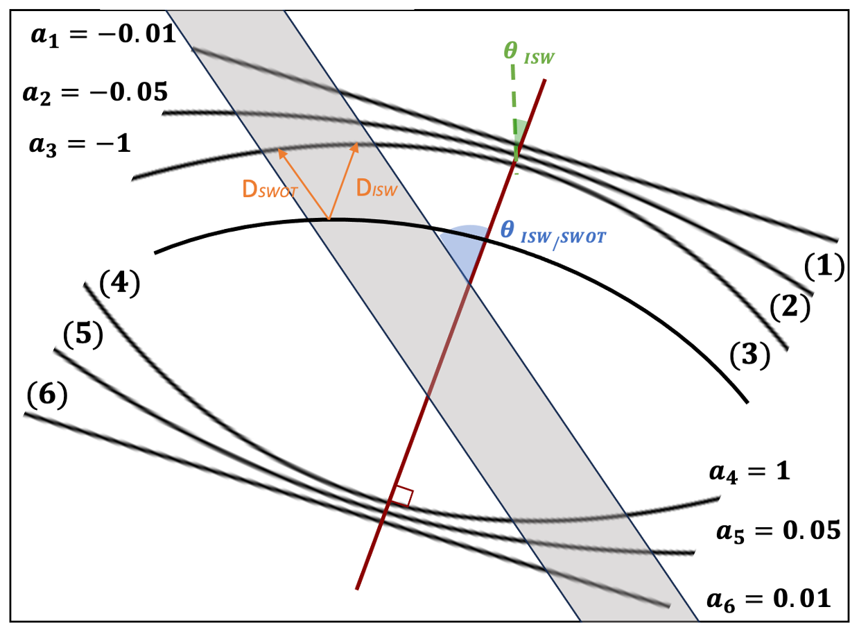
Figure 3 Schematics of wave crest characterization parameters. The red line indicates the propagation axis, θ_ISW represents the azimuth, a is an indicator of curvature and geometry of crest, ${\mathit{\theta }}_{\mathrm{ISW}/\mathrm{SWOT}}$ represent the angle beetween SWOT track (grey rectangle) and ISWs propagation axis. D_SWOT and D_ISW represente crest to crest distance, in SWOT referentiel and ISWs propagation referentiel respectively.

Finally, the distance between successive ISWs crests along the SWOT track (D_SWOT) is obtained from spectral analysis. Since ISWs are highly anisotropic and the propagation direction of the ISW packets is not always aligned with the SWOT track. In order detect the ISW wavelength, one needs to apply a rotation of  ${\mathit{\theta }}_{\mathrm{ISW}/\mathrm{SWOT}}$ which represents the angle between the ISW propagation direction and the SWOT track direction. The crest-to-crest distance of the  ISWs (D_ISW) can be determined as Eq. (2):

$$\begin{array}{}\text{(2)}& D_{\mathrm{ISW}}=D_{\mathrm{SWOT}}\cdot \cos {\mathit{\theta }}_{\mathrm{ISW}/\mathrm{SWOT}}\end{array}$$

4 Results

4.1 Three eddy cases within the ISW propagation region

The objective of this study is to understand how mesoscale eddies influence the directional changes of ISWs propagating through the region (Fig. 4, ISWs area indicated with a gray contour). To achieve this, three representative cases were selected:

• Case 1: No Eddy interaction (NE) – Characterized by the absence of mesoscale eddies within the ISW propagation pathway, observed on 14 March 2024 (Fig. 4a).

• Case 2: Cyclonic Eddy interaction (CE) – A cyclonic eddy was present near a seamount, centered at 4.96° N, 43.08° W, on 29 September 2023 (Fig. 4b).

• Case 3: Anticyclonic Eddy interaction (AE) – An anticyclonic eddy, also located near the seamount, was centered at 4.11° N, 42.76° W, on 22 August 2024 (Fig. 4c).

These scenarios provide a suitable framework for analyzing the diverse interactions between ISWs and mesoscale eddy structures, and for assessing how such interactions modulate ISWs trajectory, geometry, and propagation behavior.

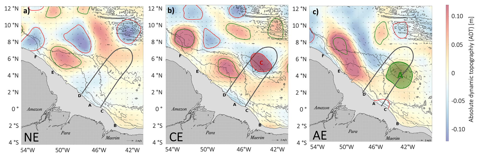
Figure 4 Eddy detection map based on MIOST L4 filtered ADT with a 1000 km cutoff for 3 cases (a) No eddies in ISWs propagation area 14 March 2024 (b) Cyclonic eddy in ISWs propagation area 29 September 2023 (c) Anticyclonic eddy in propagation area 22 August 2024. Cyclonic eddies (C) and anticyclonic eddies (A) are marked by red and green circles, respectively. Grey contours delineate the typical area where ISWs are found propagating from sites A and D. Black arrows represent geostrophic velocities. NE = no eddy interaction; CE = cyclonic eddy interaction; AE = Anticyclonic eddy interaction.

The three cases occur close to neap tides minima (Fig. 5). These minima are predicted by the FES2012 tidal model, based on the dominant M2 and S2 components within the AMAZONE36 domain. During these moments, energy levels are relatively low and comparable across cases. This conFiguration enables a coherent analysis of ISW energy variations by minimizing the influence of tidal variability.

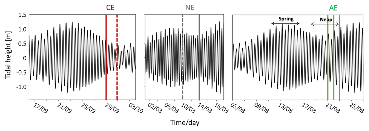
Figure 5 Barotropic tide prediction based on M2 and S2 harmonics from FES_M2_S2 AMAZONE36. Solid lines indicate the dates of the 3 show cases identified on SWOT and MIOST data (NE, CE, AE). Dotted lines indicate the date of sunglint data acquisition. NE = no eddy interaction; CE = cyclonic eddy interaction; AE = Anticyclonic eddy interaction.

4.2 Signature of ISW, refraction and diffraction from the interaction with eddies

For each case it is essential to confirm that the signatures observed in SWOT (ADT_swot) are caused by ISWs. To do so, we use sunglint images with broader spatial coverage. This helps distinguish ISWs from other features such as fronts or filaments. MODIS Aqua and NOAA-20 optical images (Fig. 6a, b, c) clearly reveal a succession of crests in all three cases. These crests appear as alternating bands of increased and decreased sea surface roughness. This pattern is consistent with ISW signatures described in previous studies (Alpers, 1985; Silva et al., 2011; de Macedo et al., 2023). ISWs crest show spatial regularity. They repeat coherently within the region of high ISW activity (Fig. 6, grey area). As observed by de Macedo et al. (2023) (Fig. 1b, black dots), ISWs follow a straight path from the continental slope offshore before interacting with the mesoscale structures. In the first case (NE), SWOT and sunglint sample ISWs initially propagating from site A (Fig. 6a and d). In the two other cases (CE and AE), sunglint images (Fig. 6b and c) and SWOT data (Fig. 6e and f) show a convergence of ISWs generated at sites A and D between 3–5° N and 44–46° W. These ISWs follow oblique propagation trajectories and eventually converge, forming a distinct V-geometry wave crest toward the eddy region.

From these images, we derive a key result of this study: after interacting with mesoscale eddies, ISWs follow distinct trajectories in each of the three analyzed cases. In the NE case, sunglint (Fig. 6a) and SWOT data (Fig. 6d, pass 227) show a straight propagation path up to 12° N (Fig. 6a, orange arrow). In contrast, in the CE case (Fig. 6e, pass 227; Fig. 6b), the ISWs are refracted northwestward after interacting with the cyclone (Fig. 6b, top orange arrows). In the AE case, the ISW resulting from the convergence splits into two branches as it approaches the western edge of the anticyclone. One branch is refracted northward (Fig. 6f, pass 074), while the other is refracted eastward (Fig. 6f, passes 046 and 018; Fig. 6c). This eastern branch appears to follow the northern edge of the anticyclone, and NECC current. Further east, near 45° W, a third refracted branch is visible, also directed northward (Fig. 6f, pass 046).The three cases offer a clear and contrasted sample of the diverse responses resulting from these complex interactions.

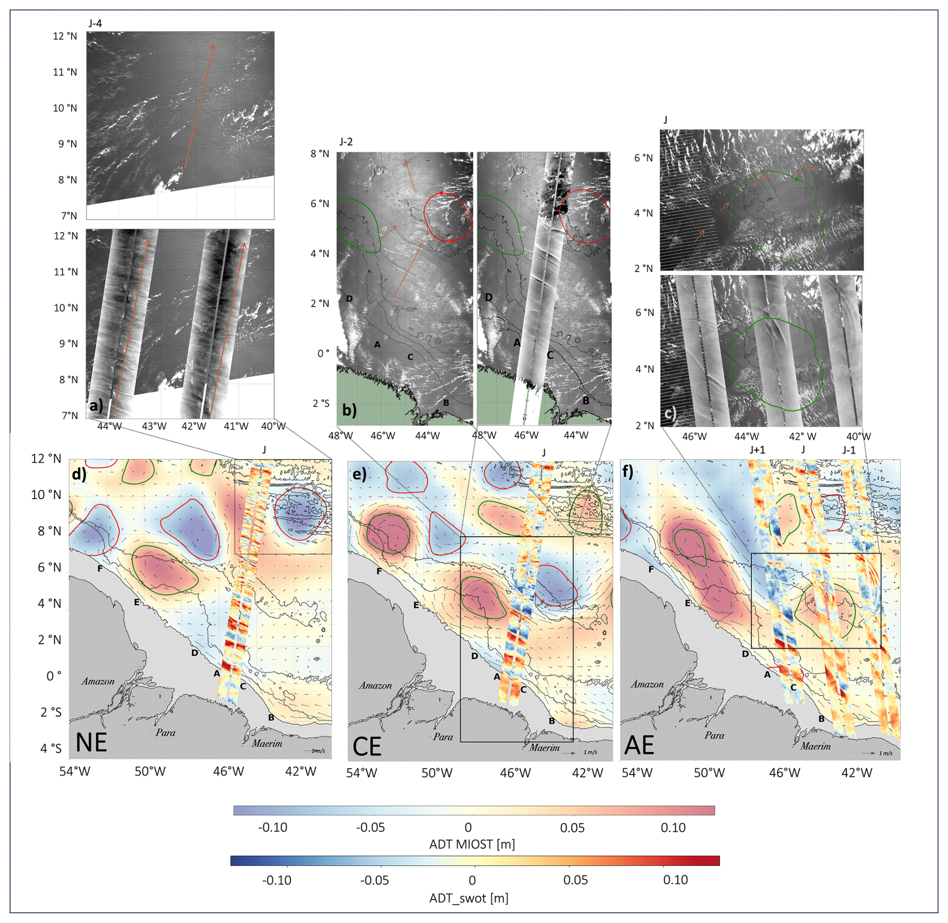
Figure 6 Eddy detection maps based on MIOST L4 ADT (filtered with a 1000 km cutoff) and ADT_swot SWOT L3, combined with Level 1B ptical imagery and SWOT sigma0 data: (a) MODIS-Aqua (10 March 2024) (b) MODIS-Aqua (1 October 2023) (c) NOAA-20 (22 August 2024) (d) SWOT cycle 012, pass 227 (14 March 2024) (e) SWOT cycle 020, pass 227 (29 September 2023) (f) SWOT cycle 020, passes 018, 046, and 074 (21–23 August 2024). Cyclonic eddies (C) and anticyclonic eddies (A) are marked by red and green circles, respectively. NE = no eddy interaction; CE = cyclonic eddy interaction; AE = Anticyclonic eddy interaction. Bathymetry is represented using isocontours at −3500, −3000, −100, and 0 m.

4.3 Impact of eddies on ISW characteristics

4.3.1 Spectral analysis: ISWs mean characteritics

The extraction of ISW crests on SWOT ADT_swot field reveals the geometry of ISW and provides an initial insight into their response upon interaction with eddies. In this section, we present the results of the detection method described in Sect. 2.2. Each track was divided into several regions associated with different dynamics before and after interaction with the eddies (Fig. 7, Table 1).

Table 1 Characteristics of ISWs detected during (NE) 13 March 2024, (CE) 29 September 2023 and (AE) 22 Augst 2024.

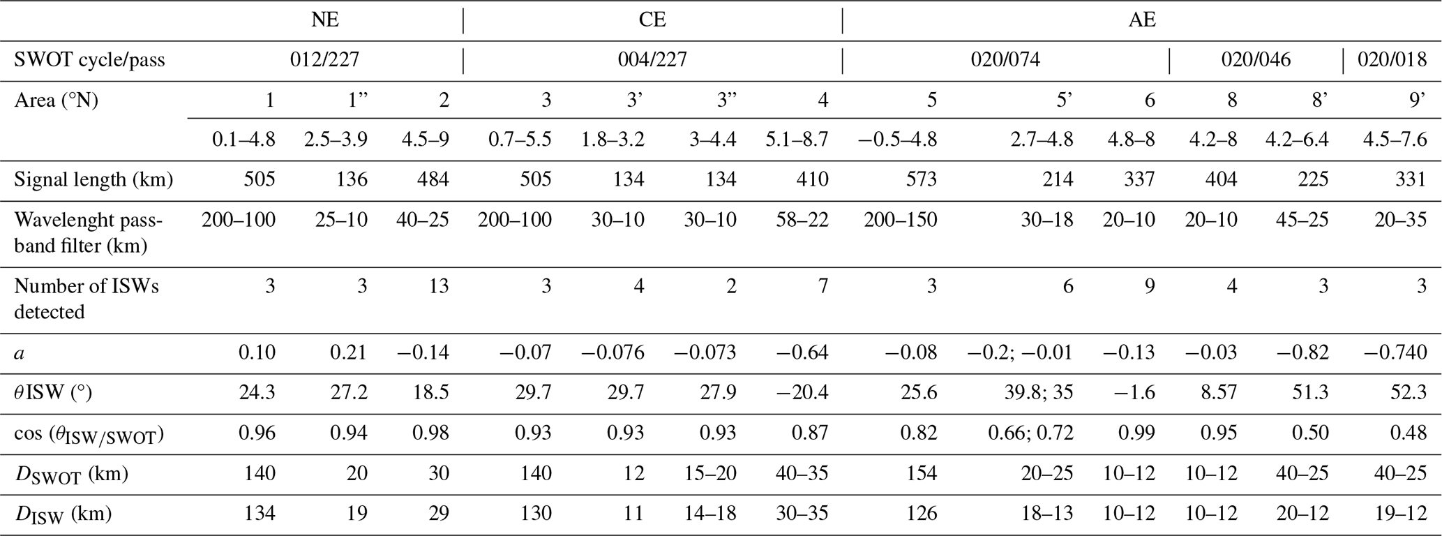
Before any interaction with the seamount or the eddies, three packets of ISWs were detected, exhibiting relatively large crest ADT signatures. In the NE case, the main crests reach ADT amplitudes between 10 and 14 cm (Fig. 7g). In the CE case, ADT amplitudes range from 6.3 to 8.5 cm (Fig. 7h), while in the AE case they vary between 4.7 and 8.6 cm (Fig. 7i).

After crossing the seamount, the NE case shows 13 crests (Fig. 7g), whose surface expression is reduced, with ADT amplitudes between 3 and 8 cm (Fig. 7g). In the CE case, the interaction with the cyclone leads to the detection of 7 crests (Fig. 7h) in the refracted wave field, with an average ADT amplitude of about 5.8 cm (Fig. 7h). In the AE case, the diffracted wave field to the north contains 9 crests (Fig. 7i) sampled by track 074 and 4 crests along track 046, with a low ADT signature of 0.2 cm. The refracted wave field to the east includes 3 crests sampled along track 046 and another 3 crests along track 018. These ISWs nevertheless remain energetic, with ADT signatures of 6.1 and 9.3 cm, respectively (Fig. 7i).

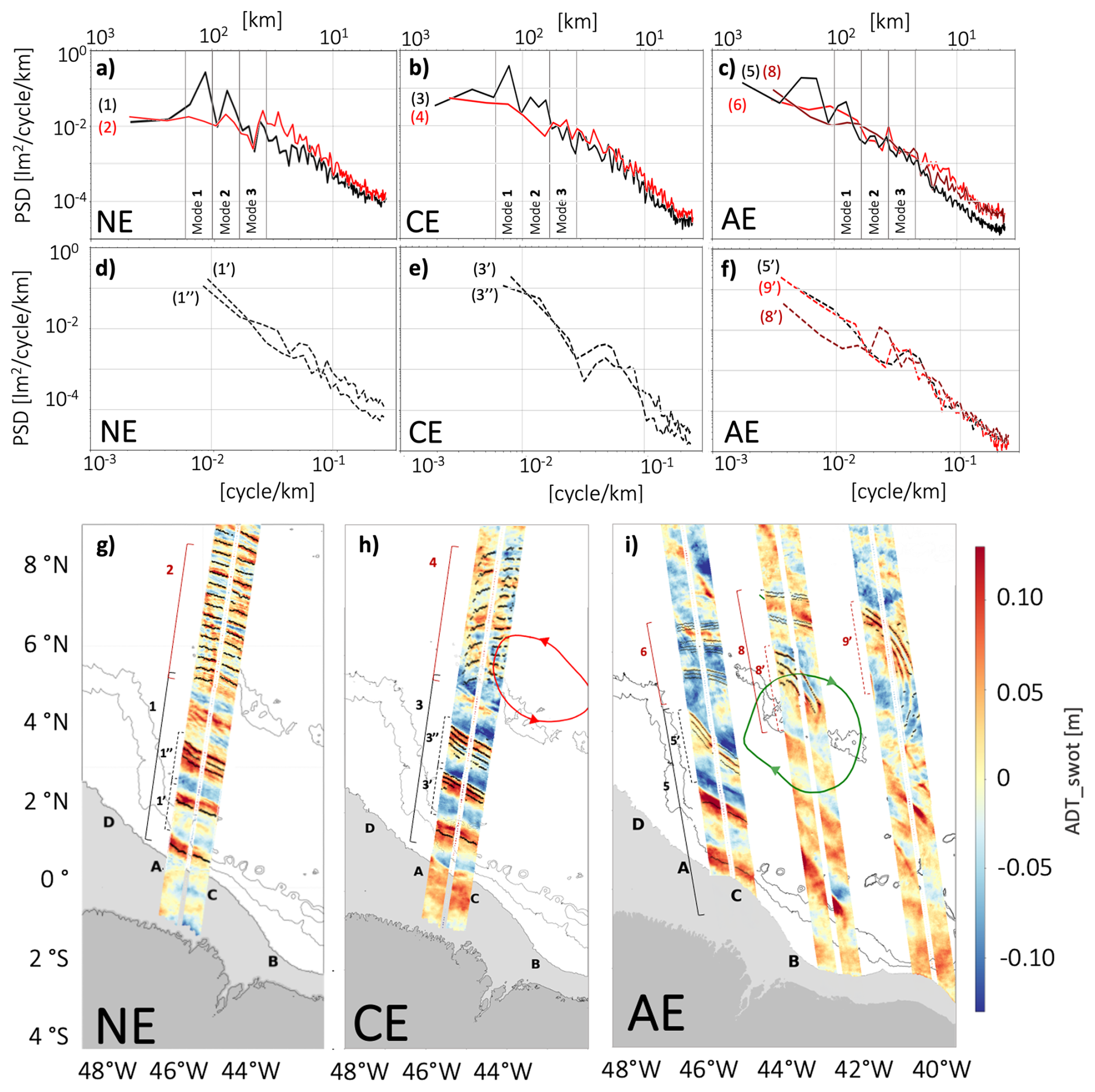
Figure 7 Mean power spectrum density of SWOT ADT_swot along track for each area for (a) NE 14 March 2024 (b) CE 29 September 2023 (c) AE 22 August 2024 (solid line). Black (red) lines refer to spectrum located before (after) interaction with seamount and eddy. Mean power spectrum density of SWOT ADT_swot along track for each area for (d) NE 14 March 2024 (e) CE 29 September 2023 (f) AE 22 August 2024 for a single wave packet (dotted line). Area number is indicated between parenthesis. ADT_swot with ISWs detection for (g) NE 14 March 2024 (h) CE 29 September 2023 (i) AE 22 August 2024. NE = no eddy interaction; CE = cyclonic eddy interaction; AE = Anticyclonic eddy interaction. Bathymetry is represented using isocontours at −3500, −3000, −100, and 0 m.

4.3.2 Spectral analysis: dominant wavelength

The spectral analysis of the ISWs fluxes sampled before seamount/eddy interaction area (Fig. 7a, b, c; black spectrum) shows similar patterns: each spectrum highlights two peaks at wavelengths of 170–140 and 75 km, corresponding to modes-1 and 2 IT wavelengths, respectively.

A major finding is that after crossing the seamount and interacting with eddies, the spectral analyses of the three cases differ markedly. None of the spectra show peaks associated with mode-1 IT wavelengths between 180 and 100 km (Fig. 7a, b, c; red spectrum). All spectra exhibit high energy levels at smaller scales. Specifically, in the NE case, after the ISWs cross the seamount, the spectrum shows elevated energy at scales below 50 km, with peaks between 30–40, suggesting the presence of mode-3 IT (Fig. 7a; red spectrum #2). For CE case, spectrum shows highers peaks between 50 and 25 km (Fig. 7b; red spectrum #4). For AE case, the spectra of the branches refracted to the north display generally higher energy levels at wavelengths below 30 km (Fig. 7c; red spectrum #6 and #8).

Then, the analysis was extended to characterize wave trains detected in SWOT data.In NE case, the wavelength spectra show no important peaks in area 1^′, indicating the absence of secondary structures near the principal wave crest in ISWs packet (Fig. 7d, black spectrum #1'). But the spectra around the next individual ISWs packets from A-D flux are dominated by components at 20 km (Fig. 7d, black spectrum #1”) . In CE case, the spectra around individual ISWs packets from A-D flux are dominated by components at 12 km (Fig. 7e, black spectrum #3') and by peacks around 20 km (Fig. 7e, black spectrum #3”). In the AE case, the spectra associated with the eastward-deflected branch (Fig. 7f, black spectrum #8' and #9') and with the main flux from A to D (Fig. 7f, black spectrum #5') show energy peaks between 20 and 40 km in wavelength

4.3.3 Crest to crest distance variability and ISWs-mode shifts

The wave crest detection shows that, in all three cases, the ISWs generated close to the IT source sites exhibit inter-packet distances comparable to the wavelength of IT mode-1 aroud 130 km. (Fig. 7g, h, i). In NE case, wave packet signature is observed before seamount with crest-to-crest distance around 19 km (Fig. 7g).

In addition, in case CE, where the fluxes from sites A and D converge, wave packet signatures emerge with decreasing crest-to-crest distances, ranging from 14 km down to 18 km away from the carrier wave (Fig. 7h, areas 3^′′ and 3^′). Similarly, in case AE (Fig. 7i), the merging of A and D fluxes is associated with wave packets signature characterized by distances between crest ranging from of 13–18 km (Fig. 7i, area 5^′).

After the interaction with eddy or seamount, the distance between wave packets differs significantly across the three cases. In NE (Fig. 7g), the wave crests are spaced approximately 30 km (Fig. 7g, area 2), suggesting a transformation from IT-mode-1 to IT mode-3. In CE, the distance between crests in the refracted flux are shorter than in the incident flux, around 30–35 km (Fig. 7h, area 4). In AE, the portion of the flux that is refracted northward shows waves packets with 10–12 km crest spacing inside each wave packet. (Fig. 7i, area 6). Due to data gaps between SWOT ground tracks, it is not possible to resolve the wavelengths of the flux from A that is deflected eastward by the anticyclone. However, we identify ISWs wave packets sea surface signature. The main wave gradually degenerates into smaller secondary waves characterized by distance between crests between 20 and 12 km (Fig. 7i, areas 8^′ and 9^′). Finally, the third branch, refracted northward along the edge of the anticyclone, is characterized by a short distance between crests of 10–12 km (Fig. 7i, area 8)

4.3.4 Wavecrest geometry and direction of propagation

After reconstructing the wave crests using a second-degree polynomial fit, it is observed that in the NE case, the ISWs corresponding to IT mode-1 generated at sites A and D propagate northeastward θ_ISW1 =24° (Fig. 8, area 1, black circles). The wavecrest has a relatively plane geometry, with an average curvature coefficient of a₁=0.10. During the crossing of the seamount, the propagation direction remained unchanged ($\mathrm{\Delta }{\mathit{\theta }}_{\mathrm{ISW}\mathrm{1}-\mathrm{2}}<\mathrm{6}$°) (Fig. 8, area 2, red circles). However, a decrease in the coefficient a is observed, reaching an average of $a_{\mathrm{2}}=-\mathrm{0.14}$ (Fig. 8, area 2, red circles). This indicates an increase in curvature and a more pronounced concavity of the wavefront.

In the CE case, the waves sampled before interaction also propagate northeastward, with θ_ISW3=29° and an average curvature coefficient of $a_{\mathrm{3}}=-\mathrm{0.07}$ (Fig. 8, area 3–3^′′–3^′, black triangles). These characteristics are similar to those observed in the NE case. After interaction with the cyclone and the seamount, a significant change in propagation direction is observed: the wavecrest is refracted by $\mathrm{\Delta }{\mathit{\theta }}_{\mathrm{ISW}\mathrm{3}-\mathrm{4}}=\mathrm{50}$° toward the west. The crests of the refracted ISWs then propagate northeastward, with ${\mathit{\theta }}_{\mathrm{ISW}\mathrm{4}}=-\mathrm{20}$° (Fig. 8, area 4, red triangles). Compared to the reference case, this deflection cannot be attributed to bathymetric effects, supporting the hypothesis that the refraction is induced by the cyclone. Furthermore, a strong increase in curvature is measured, reaching $a_{\mathrm{2}}=-\mathrm{0.64}$ (Fig. 8, area 4, red triangles), nearly ten times higher than that of the incident wavefront.

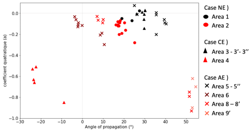
Figure 8 Orientation relative to azimuth as a function of the quadratic coefficient a of the ISWs wave crest detected. Each point represents an individual ISW wave crest detected in (A) NE 14 March 2024 (B) CE 29 September 2023 (C) AE 22 August 2024. Black and red colors represent ISWs before and after interactions with seamount/eddies, respectively. For AE case brown color indicates ISWs refracted northward, red color indicates ISWs on top off anticyclonic eddy and salmon color indicates ISWs refract eastward.

In the AE case, the ISWs originating from point A initially propagated northwestward with ${\mathit{\theta }}_{\mathrm{ISW}\mathrm{5}-\mathrm{east}}=\mathrm{25}$°. These waves encountered those from site D, which propagated at ${\mathit{\theta }}_{\mathrm{ISW}\mathrm{5}{}^{\prime }-\mathrm{west}}=\mathrm{40}$° (Fig. 8, area 5^′ – west, black cross). The wavecrest exhibited a relatively plane geometry ($a_{\mathrm{5}}=-\mathrm{0.07}$) (Fig. 8, area 5, black cross. Near the eastern edge of the anticyclone, ISWs packet was refracted northward. The first three reconstructed crests were characterized by increased curvature ($a_{\mathrm{6}}=-\mathrm{0.23}$), then, during their northward propagation, the ISWs gradually flattened, eventually exhibiting a curvature similar to that of the incident ISWs ($a_{\mathrm{6}}=-\mathrm{0.08}$) (Fig. 8, area 6, brown cross) and an azimuth of ${\mathit{\theta }}_{\mathrm{ISW}\mathrm{6}}=-\mathrm{2}$° (Fig. 8, area 6, brown cross). According to two scenarios, if the ISW branch originates from site A, it refracts northward with $\mathrm{\Delta }{\mathit{\theta }}_{\mathrm{ISW}\mathrm{5}-\mathrm{east}-\mathrm{6}}=\mathrm{27}$°. In contrast, if it originates from site D, the refraction is stronger, with $\mathrm{\Delta }{\mathit{\theta }}_{\mathrm{ISW}\mathrm{5}-\mathrm{west}-\mathrm{6}}=\mathrm{42}$°. An other part of the incident ISWs packet was refracted eastward and propagated along the edge of the anticyclone with ${\mathit{\theta }}_{\mathrm{ISW}\mathrm{8}{}^{\prime }\mathrm{\&}\mathrm{9}{}^{\prime }}=\mathrm{51}$° (Fig. 8, areas 8^′–9^′, red cross). According two scenarios, if it come from site A, ISWs was refract with $\mathrm{\Delta }{\mathit{\theta }}_{\mathrm{ISW}\mathrm{5}-\mathrm{east}-\mathrm{8}{}^{\prime }}=\mathrm{27}$°. In contrast if ISWs provide from site D it refract with $\mathrm{\Delta }{\mathit{\theta }}_{\mathrm{ISW}\mathrm{5}-\mathrm{west}-\mathrm{8}{}^{\prime }}=\mathrm{12}$°. The wavefronts in this region exhibited the highest curvature values, with a coefficient of $a_{\mathrm{8}\mathit{\&}\mathrm{9}}=-\mathrm{0.8}$ (Fig. 8, areas 8^′–9^′, red cross). Part of ISWs was refracted northward with $\mathrm{\Delta }{\mathit{\theta }}_{\mathrm{ISW}\mathrm{8}{}^{\prime }-\mathrm{8}}=\mathrm{43}$,5 (Fig. 8, area 8, red cross), and the wavefronts were characterized by a plane front $a_{\mathrm{8}}=-\mathrm{0.013}$.

These three cases demonstrate that the ISWs originating from sites A and D were relatively plane and that the combined effects of the seamount and the refraction induced by the cyclonic and anticyclonic eddies deflected the wave trajectories and modulated the crest curvature.

5 Discussion

5.1 Convergence of A and D fluxes favors ISW formation

5.1.1 Convergence region as a mixing hotspot

In our study, we observe that the ISWs emitted from sites A and D predominantly exhibit an inter-packet spacing characteristic of mode-1 IT and converge in both case studies (AE and CE) between 3–5° N and 44–46° W. These results are in good agreement with modeling outcomes (Tchilibou et al., 2022) that demonstrated this convergence, as well as the study by de Macedo et al. (2023), which identified the convergence region of these fluxes as a hotspot of intense mode-1 ISW activity. Ultimately, this convergence region may play a role in mixing intensification, as suggested by the work of Kouogang et al. (2025a), based on recent direct in-situ measurements from the AMAZOMIX program.

5.1.2 Oblique wave-wave interaction

In the interaction region between fluxes A and D, we observe a V-geometry wave crest suggestive of an oblique interaction in both AE and CE cases. According to the literature (Yuan et al., 2018, 2023; Wang and Pawlowicz, 2012; Helfrich, 2007; Shimizu and Nakayama, 2017), oblique interactions described here can mainly be indentified in two forms:

A merging of wave packets leading to the formation of a longer packet (Fig. 9a),

Both solitary wave packets passing through each other without significant alteration in geometry or amplitude (Fig. 9b).

In our study, for the AE case, following the oblique interaction between ISWs originating from sites A and D, the lack of data just after the convergence point prevents us from concluding the type of interaction and the subsequent ISW trajectories. Several scenarios are possible. It could involve a merging of wave fronts (Fig. 9a) followed by divergence under the influence of an anticyclone: ISWs from A could be deflected eastward, while those from D would be deflected westward. A second possible scenario in the AE case (Fig. 9b) is that ISWs from A and D meet, cross paths, and are deflected in opposite directions – northward for those from A, and eastward for those from D.

The different case studies in our research illustrate the complexity of possible outcomes and suggest that the offshore Amazon region is particularly favorable for studying these complex nonlinear wave interaction phenomena.

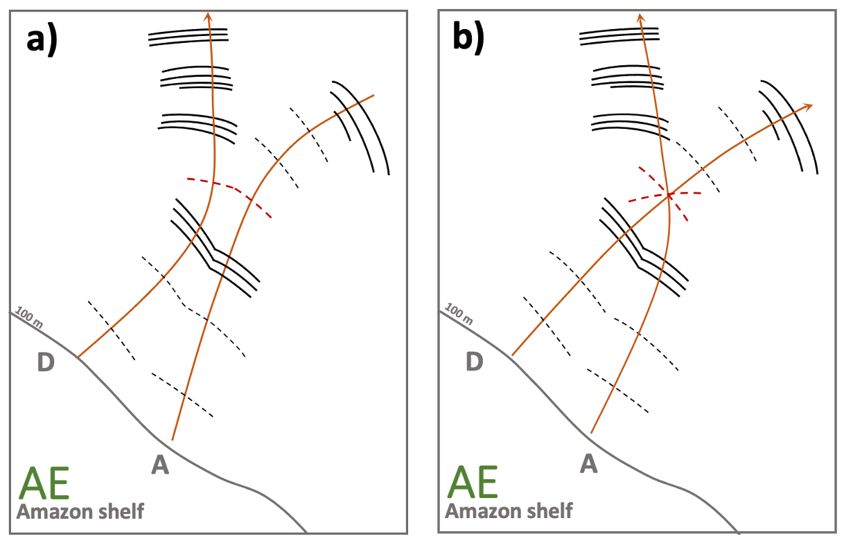
Figure 9 Interaction between ISWs detected (black lines) off site A and D in AE case (22 August 2024) according to two propagation trajectory scenarios (a) divergent trajectories with hypothetic front merge (red dot line) (b) hypothetic crossing trajectories (red dot line).

5.2 Refraction and distortion of ISWs after eddy interaction

5.2.1 Separating the effects of the NECC and eddies

The NECC is closely linked to mesoscale eddy dynamics, which makes it difficult to isolate its specific impact on ISW propagation. Nevertheless, its role deserves particular attention. Indeed, in the AE case, ISWs appear to be deflected eastward toward the edge of the eddy prior to the interaction, following the NECC streamlines. This intense zonal current, with a variable path, could indeed influence ISW trajectories. This observation supports the hypothesis proposed by Tchilibou et al. (2022), de Macedo et al. (2023) and Magalhães et al. (2016) suggesting that the strengthening of the NECC plays an important role in the acceleration, refraction, diffraction and shift ITs associated to ISWs in the northeastern region.. For comparison, it has been showed that the meandering Gulf Stream significantly refracts and traps ITs (Duda et al., 2018), highlighting the ability of such a current to act as a barrier or waveguide for ITs. By analogy, the contribution of the NECC in the deflection or distortion of ISW crests cannot be overlooked using satellite observation, and a dedicated analysis would be necessary to assess its relative contribution using idealized numerical experiments.

5.2.2 Distortion of wave crests

This study shows that ISW deflections substantially increase wave crest curvature, in agreement with idealized simulations (Guo et al., 2023). This is particularly evident in the AE case, when the center of the ISW front is aligned with the current along the northern edge of the anticyclone (Fig. 10c), and in the CE case, when the ISW tip is opposed to the current along the western edge of the cyclone (Fig. 10b). Eddies feature strong gradients in both velocity and stratification, with maximum speed at the edges and minimum at the center. When ISWs interact with this spatially varying current field, their local phase speed can be altered (Lamb, 2014; Dunphy and Lamb, 2014). Some sections of the wave front may be “accelerated” where the current aligns with the direction of ISWs propagation (Fig. 10c), while others may be “slowed down” in the presence of opposing or weaker currents (Fig. 10b). This spatial variation in ISW phase speed leads to significant distortion of the wave front, which becomes markedly more curved than the initially planar incident front.

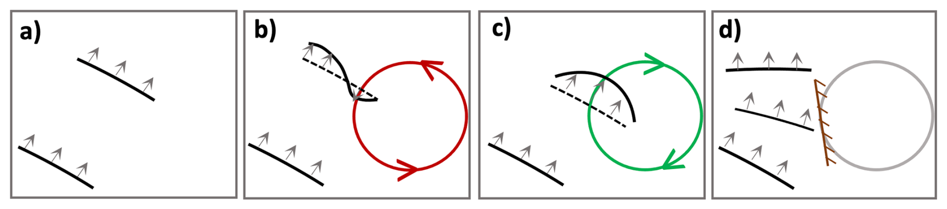
Figure 10 Impact of eddy edge currents on the curvature of internal wave crests for (a) No eddy interaction (b) Cyclonic eddy interaction (c) Anticyclonic eddy interaction (d) “physical wall” interaction. Cyclonic eddies and anticyclonic eddies are marked by red and green circles, respectively.

In contrast, in the AE case, after interaction, part of the ISW flux is refracted northward (Fig. 7i). This portion of the flux maintains a relatively flat curvature throughout its propagation. One possible explanation for the absence of wavefront distortion after refraction is that the ISWs do not interact directly with the intense edge currents of the eddy, but are instead reflected upon encountering a kind of “physical wall” (Fig. 10d). This interpretation is supported by recent studies (Guo et al., 2023; Wang and Legg, 2023), which show that stratification changes induced by eddies can refract ISWs.

This observation contributes to an ongoing debate within the scientific community regarding the relative roles of stratification and currents in the processes of internal tide refraction and ISW distortion. Several studies (Bendinger et al., 2025; Guo et al., 2023; Wang and Legg, 2023; Xu et al., 2024) suggest that eddy-related currents play the dominant role in ISW refraction, relegating the effect of local stratification variations to a secondary role. However, in other oceanic contexts, it is precisely these stratification changes that appear to be the main driver of internal tide refraction and coherence loss, surpassing the influence of relative vorticity gradients and subtidal currents (Zaron and Egbert, 2014). These findings highlight the importance of regional conditions and the complex interaction between stratification and currents in shaping ISW trajectories and behavior.

5.3 Satellite Data Limitations

5.3.1 Uncertainty in the spatial and temporal positioning of eddies

The scenarios explored underscore the need for accurate estimates of eddy locations to assess their influence on ISW dynamics. However, uncertainty exists regarding the precise positioning of these eddies. They are identified from daily altimetric maps that combine measurements from several satellites passing at different times. The interpolation of these data inevitably leads to smoothing of small scales and a loss of spatial and temporal resolution. Consequently, when compared with instantaneous measurements from SWOT and MODIS/NOAA20, it becomes difficult to determine whether the ISW–eddy interaction occurs at the eddy core or periphery. This uncertainty can limit the interpretation of observations.

5.3.2 Satellite Sampling

In the AE case, the lack of data between SWOT tracks prevents observation of the wavefront evolution after the wave–wave interaction. This makes it impossible to precisely characterize the type of wave–wave interaction and also limits observations of wave–eddy interactions.

More generally, several factors hinder the observation of wave–eddy interactions: the temporal resolution of satellite sensors, environmental conditions (cloud cover, wind, ocean surface state, sun angle), and the viewing angle. These limitations also affect the interpretation of physical processes, including ISW refraction and the detection of ISW packets. In unfavorable conditions, only the leading wave with strong contrast is visible in sunglint or σ⁰ images.

Additionally, what is interpreted in the CE case as westward refraction of the wave flux by the cyclone may in fact only represent part of a diffracted wave flux, of which only the western branch is captured. Other branches to the east may exist but are unfortunately not captured in our case studies. Therefore, we cannot conclude on the full extent of the flux, as satellite images do not capture it in its entirety.

Finally, satellite altimetry and surface geostrophic velocities primarily capture the barotropic signal and the baroclinic mode-1 structure, which remains a substantial limitation for the detection and characterization of baroclinic eddies. Yet, the vertical structure and intensity of baroclinic eddies likely condition their interactions with the surrounding flow and with propagating internal solitary waves, potentially leading to distinct dynamical responses. Our results provide qualitative and first-order evidence of eddy–ISW interactions as observed by SWOT, but the absence of in situ measurements prevents us from assessing the vertical structure of the eddies involved. It is therefore reasonable to expect that these interactions may differ when eddies exhibit a more complex vertical configuration, such as a dipolar structure, and future work should aim to resolve and analyze this vertical structure to better quantify these processes.

These observational limitations may lead to an underestimation of the extent and complexity of eddy-induced ISW modifications and emphasize the need to complement the analysis with in situ measurements or 3D high-resolution modeling to better capture the full scale and dynamics of ISWs and their interactions with eddies

5.4 Inter-packet Distance and Mode Transfer

5.4.1 Effect of the Seamount

In the NE case, an energy transfer from mode-1 IT to higher IT modes, particularly mode-3, was observed. This phenomenon aligns with numerous studies showing that steep bathymetry can disperse internal tide energy into higher modes and enhance mixing (Johnston and Merryfield, 2003; Johnston et al., 2003; Mathur et al., 2014). One hypothesis is that the presence of a seamount can locally alter stratification and the effective water column depth, thus affecting internal wave phase speed and reducing wavelength. A broader analysis of SWOT data would be valuable to systematically confirm the impact of topography on ISW behavior.

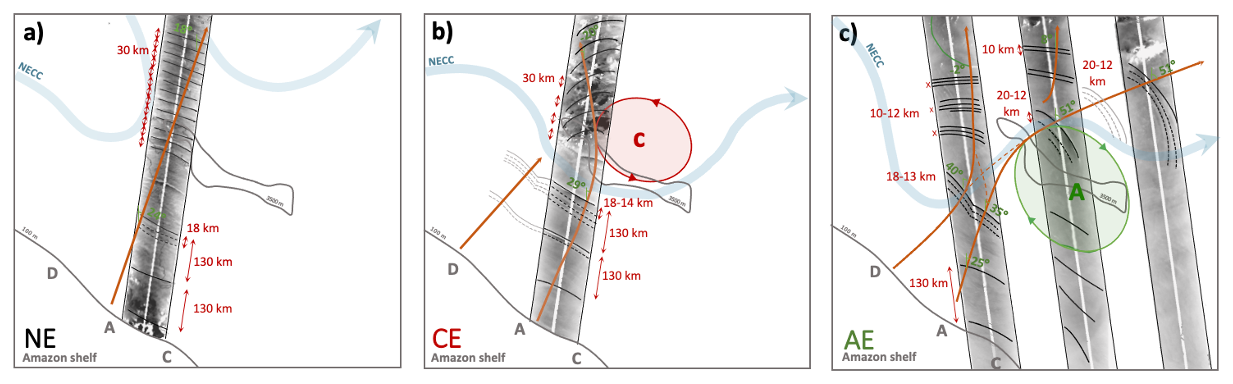
Figure 11 Interaction between ISWs detected (black lines) off site A and D for (a) NE 14 March 2024 (b) CE 29 September 2023 (c) AE 22 August 2024 on sigma0 SWOT data. Grey lines denote ISWs visible on MODIS and NOAA-21 sunglint images. Orange line denotes axis of propagation. Red line show crest-to-crest distance (D_ISWs).

5.4.2 Combined Effect of the Seamount and Eddies

In addition to the effect of seamounts, a similar mode transfer from mode-1 to mode-3 was observed during wave deflection by a cyclone. These findings are consistent with earlier studies (Guo et al., 2023; Dunphy and Lamb, 2014), which demonstrated that a mode-1 internal tide interacting with an eddy can transfer energy to higher modes, thus reducing the main mode's energy flux. Moreover, in the AE case, we observe the emergence of wave trains (three crests following the main one, with inter-packet distances on the order of 10 km) in the deviated branch after interaction with the anticyclone. In contrast, in the NE case, the main crest appears alone, i.e., without a trailing wave train. Our results raise the hypothesis that the eddy may destabilize the ISW's main crest and enhance wave train formation. More quantitative studies are needed to refine this hypothesis.

5.5 Detection Method and Perspectives

The method used in this study to detect ISW wavefronts is innovative and would benefit from automation. However, this approach presents several limitations that currently prevent its generalization. It is particularly sensitive to the choice of analysis window size, changes in wavelength, and the presence of submesoscale processes also visible in SSH, which remain difficult to automatically separate. Additionally, the choice of filtering window size affects detection precision. Nevertheless, characterizing ISWs based on their morphology offers a promising avenue for detecting and isolating these structures in SSH fields observed by SWOT, especially when coupled with σ⁰ measurements.

6 Conclusions

This study investigates the impact of mesoscale eddies on the characteristics of ISWs off the Amazon Shelf, focusing on their distance between crests, mode, propagation direction, and crest curvature. The analysis is based on the extraction of ISW signals from SWOT L3 KaRIn wide-swaths measurements, and the identification of eddies from daily MIOST ADT maps. Three distinct interaction scenarios were analyzed: a case of propagation without interaction, a case of refraction by a cyclonic eddy, and a case of diffraction by an anticyclonic eddy.

It was shown that, prior to any interaction with eddies or bathymetric features, the ISWs generated from ITs whose origins are sites A and D propagated with angles ranging from 25 to 28° relative to the north-south axis. The wavefronts exhibited ADT amplitude beetween 5 and 14 cm, plane geometries and were dominated by crest spacing corresponding to wavelength of IT mode-1. The presence of a seamount did not affect ISWs propagation but induced a shift toward crest spacings characteristic of IT mode-3 (Fig. 11a) and a decrease in the ADT amplitude down to values as low as 8 cm. In contrast, interaction with the western edge of a cyclonic eddy and seamount resulted in a 50° westward refraction of the wave train. This interaction was accompanied by a significant increase in crest curvature and a reduction in ADT amplitude and inter-packet distance, indicating a shift toward crest-to-crest distances consistent with IT mode-3 (Fig. 11b). Finally, interaction with the western edge of an anticyclonic eddy and seamount led to diffraction. One branch of ISWS refracted westward, a minimal ADT amplitude close to 0.2 cm and exhibiting flatter wave crests, and several waves packets. Simultaneously the other ISWs branch was deflected eastward, with the crests becoming highly curved and wave packets emerging marked by an ADT amplitude reaching 9.3 cm (Fig. 11c)

This study provides the first observational evidence of ISWs refraction and diffraction after ISWs interact with eddies of different polarity. The detection method developed in this study proved promising in highlighting the diversity of ISW responses regarding eddy structures and location with respect to the ISW path. As a continuation, applying this approach to other regions and case studies would be valuable in broadening our understanding of ISW/eddy interaction variability. The 250 m SWOT data might also be used to reveal other fine scales features of the ISW and their interactions with eddies. A comparison with results from idealized and ray-tracing experiment that simulates the horizontal propagation of internal tidal rays tthrough a mesoscale eddy field might highlight the IT propagation direction.

Appendix A: Sensitivity tests

Each SWOT track was subdivided into several windows. In this appendix, we assess the sensitivity of ISW detection to the window size (ranging from 200 to 850 km). For demonstration purposes, we focus on mode-1 ISWs, though the results are similar for other wavelengths. Figure A1 illustrates the results of these tests for pass 227, cycle 004.

For all window lengths, the associated spectra show a peak in the 100–200 km band (Fig. A1A), corresponding to mode-1 internal tides/solitary waves. This peak is clearly visible for all window lengths, except perhaps for the 275 km window (Fig. A1Aa), which truncates the spectral intensity. We conclude that window lengths greater than 275 km provide sufficient spectral resolution to isolate the structures of interest.

The identification of ISW crest positions projected onto the SWOT tracks shows that for windows between 275 and 505 km (Fig. A1Ba, b, c), there is a high correlation between the raw and filtered signal (r>0.6, Fig. A1Ca, b, c), with a low standard deviation (0.01 < σ<0.1, Fig. A1Ca, b, c) along the entire track. In contrast, for longer windows (620 to 845 km, Fig. A1Bd, e, f), the correlation drops beyond 500 km (r < 0.6, Fig. A1Cd, e, f), and the standard deviation increases (0.01 < σ < 0.3, Fig. A1Cd, e, f). This drop in correlation is likely related to additional high-frequency submesoscale processes (Fig. A1Bd, e, f, grey curve).

Furthermore, for the smallest window (275 km, Fig. A1Aa), the correlation over the first 100 km is $r=\mathrm{0.85}\pm \mathrm{0.03}$ (Fig. A1Ca), while for the longest window (845 km), it reaches $r=\mathrm{0.90}\pm \mathrm{0.02}$. This is likely due to edge effects caused by the implicit periodicity assumption of the Fourier transform. These effects are limited because the start of the window coincides with the beginning of the ISWs. Additionally, although spectral truncation can theoretically produce edge artifacts (Gibbs phenomenon), no such artifacts were observed in our tests.

We conclude that, in this case, windows between 275 and 505 km (Fig. A1ab, c) allow for proper extraction of ISW crests, with limited edge effects. We select the largest valid window (505 km) as it offers the best compromise – minimizing edge effects while avoiding the inclusion of additional submesoscale processes. This choice is also supported by theoretical considerations: according to Oppenheim et al. (1996), reliable spectral analysis requires the signal length to be at least twice the target wavelength.

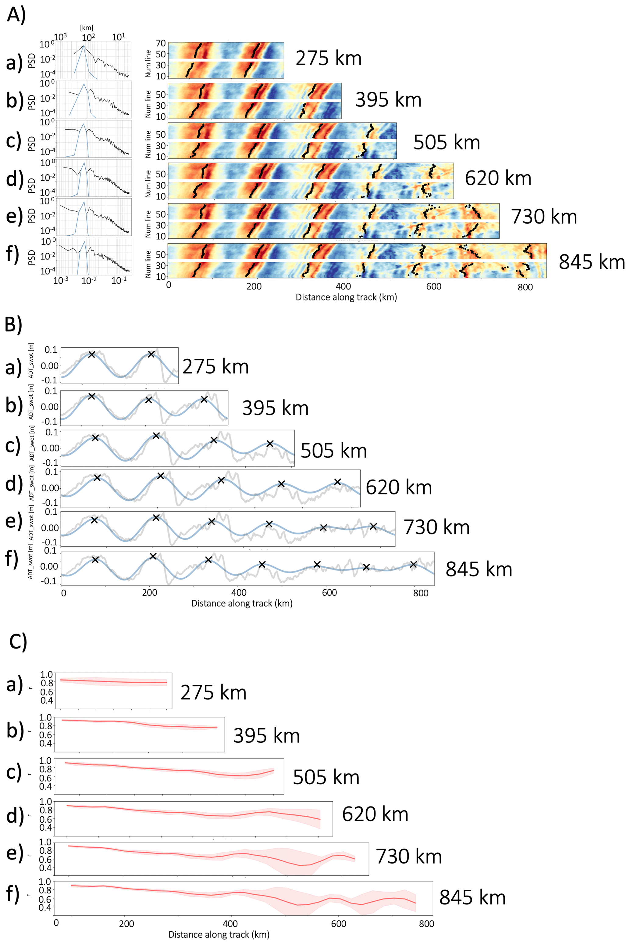
Figure A1 (A) Mean power spectral density of SWOT ADT_swot along-track and ADT_swot with ISWs detection for 6 signal lengths from 200 to 850 km. (B) The grey line represents the raw ADT_swot signal, while the blue line shows the signal filtered with a pass-band filter between 200 and 100 km along pixel line number 53. (C) Mean Pearson correlation between the raw ADT_swot signal and the filtered signal.