Characterising marine heatwaves in the Svalbard Archipelago and surrounding seas

In the Arctic Ocean, satellite-based sea surface temperature data shows that marine heatwave (MHW) intensity, frequency, duration and coverage have increased significantly in recent decades, raising concern for Arctic ecosystems. A high frequency (more than three events per year) of MHWs has been shown around the Svalbard Archipelago. Based on this, we investigate MHW trends around Svalbard at the surface and subsurface, using a regional reanalysis from TOPAZ (1991–2022). We find an increase in the frequency and duration of MHW events around the Svalbard Archipelago over the last decade. Focussing on a region west of Svalbard, we observe an increase in MHW frequency and duration, associated with a long-term rise in sea surface temperature in the region. Analysis of eight individual summer (June–September) MHW events lasting longer than 10 d west of Svalbard, indicated the presence of four shallow (≤50 m) and four deep (>50 m) MHWs after 2010, with a mean duration of 29 d. Some events extended into the Barents Sea. Heat budget analysis demonstrated a greater contribution of ocean heat transport compared to air-sea heat fluxes in driving the MHW events. Deep and shallow events were associated with ocean heat transport anomalies of up to 9 TW. This new understanding of MHW characteristics, including their horizontal and vertical distribution, is key to assessing ecological impacts.

1 Introduction

Marine heatwaves (MHWs) are characterised as prolonged periods of extreme high sea surface temperatures relative to the long-term mean daily seasonal cycle. MHWs have become more frequent due to climate change and this trend is likely to increase in the future (IPCC, 2021). Recent studies have noted that the average global annual MHW frequency and duration have increased by 34 % and 17 % respectively over the last century (Oliver et al., 2018). Severe MHWs have been detected worldwide including in the Mediterranean Sea (Ibrahim et al., 2021), northwest Atlantic Ocean (Chen et al., 2014), China Seas (Li et al., 2019) and over the Red Sea (Mohamed et al., 2021). The majority of current MHW studies focus on surface MHWs. However, MHWs also reside in the subsurface ocean (Capotondi et al., 2024; Malan et al., 2025) and are not always apparent in surface data (Sun et al., 2023). MHWs can be triggered by both local and remote atmospheric and oceanic forcings, including heat advection by ocean currents (Oliver et al., 2018), or atmospheric overheating through an anomalous air-sea heat flux (Olita et al., 2007; Chen et al., 2015).

An increase in the number and intensity of MHWs is a growing concern due to the threat to marine communities. The biological impacts of MHWs include changes in species distribution, loss of biodiversity and a collapse of habitat-forming foundation species – including reef-building corals, seagrasses and seaweeds (Smith et al., 2023). Recent MHWs have already been connected to mass mortality events of primary producers, corals and invertebrates (Filbee-Dexter et al., 2020; Garrabou et al., 2022; Shanks et al., 2020). Furthermore, studies predict that MHWs will cause a decrease in the biomass of commercially important fish species (Cheung et al., 2021). The latter are expected to have drastic socioeconomic impacts as the frequency of MHWs increases. The extent to which the impacts of MHWs are felt by fish species, however, remains unclear (Fredston et al., 2023). Additionally, MHWs have been shown to impact weather patterns, with evidence showing an intensification of storms during MHW events at lower latitudes (Choi et al., 2024).

Studies have shown increasing trends in the annual intensity, frequency, duration and areal coverage of MHWs in the Arctic Ocean (north of 60° N, Huang et al., 2021b), with regional studies highlighting notable trends in the Barents Sea (Mohamed et al., 2022) and the Siberian Arctic (Golubeva et al., 2021). Furthermore, Arctic MHWs are projected to intensify in the twenty-first century (He et al., 2024; Gou et al., 2025). The increase in MHWs in the Arctic Ocean has been linked to a rise in surface air temperatures and sea ice retreat (Huang et al., 2021b). As a result of the phenomenon known as Arctic amplification, near-surface air temperatures in the Arctic have warmed faster by a factor of three to four, compared to the global average (Rantanen et al., 2022). Concurrently, the annual mean sea-ice extent in the Arctic Ocean has decreased by 20 % since the 1980s, with the largest decline observed in summer (Eisenman et al., 2011; Stroeve et al., 2025); Arctic sea ice continues to decrease both in extent and thickness (Sumata et al., 2023) with a shift from multi-year ice to first-year ice (Comiso and Hall, 2014; Maslowski et al., 2012). The latter is a particular concern as Hu et al. (2020) found more extreme MHW events in first-year ice regions compared to multi-year ice and open-water regions. Unlike regions further south, knowledge of MHWs in the Arctic Ocean is limited and we lack a full understanding of the triggers of Arctic MHWs and their impacts on biogeochemistry (report by PlanMiljø, 2022, for the Norwegian Environment Agency).

The Svalbard Archipelago located north of the Arctic Circle at 74–81° N, 10–35° E (Fig. 1), has been shown to experience a relatively high frequency of MHWs compared to other regions of the Arctic (approximately 2–3 events per year, Huang et al., 2021b). The Svalbard Archipelago forms part of the Barents Sea shelf with an average depth of 200–300 m. Adjacent off-shelf areas exceed depths of 2000 m. The region is influenced by cold Arctic water masses formed locally in winter and advected from the northeast by the East Spitsbergen Current and further by the Spistbergen Polar Current along the coast, west of Svalbard (Fig. 1). The region is also influenced by the warm West Spitsbergen Current (WSC), which flows northwards transporting warm Atlantic Water (AW) along the slope of the West Spitsbergen Shelf (Fig. 1); here AW extends to approximately 500 m depth, with the AW maximum temperature present between 300–600 m (Menze et al., 2019). The WSC continues along the West Spitsbergen shelf-slope and then flows into the Arctic Ocean, where it circulates cyclonically.

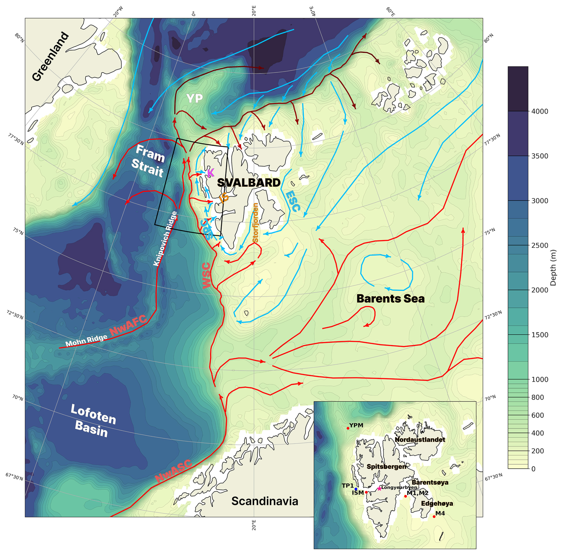
Figure 1 Schematic map of the oceanic circulation around the Svalbard Archipelago; NwASC (Norwegian Atlantic Slope Current), NwAFC (Norwegian Atlantic Front Current), WSC (West Spitsbergen Current), SPC (Spitsbergen Polar Current), ESC (East Spitsbergen Current). Blue arrows represent cold Arctic water masses, red arrows represent warm Atlantic water masses (adapted from Vihtakari et al., 2019; Eriksen et al., 2018). The darkening of the red arrows indicates where Atlantic Water becomes gradually more subsurface. Location of Kongsfjorden (K), Isfjorden (IS) and the Svalbard West domain (black box, 77–80° N, 5–15° E) are shown. Small inset map indicates the locations of the Isfjorden Mouth Mooring (ISM), TOPAZ point for validation with the ISM Mooring (TP1: 78.125° N, 11.75° E), Yermak Plateau Mooring (YPM), Storfjorden Moorings (M1, M2) and M4 Mooring. The TOPAZ bathymetry is shown.

Warm AW transported by the WSC is important for shaping the climatic conditions of the Svalbard Archipelago. The archipelago has experienced an increase in the temperature of inflowing AW, accompanied by a rise in regional sea surface temperatures. AW transported by the WSC past Svalbard has warmed, with a positive trend of 0.06 °C yr⁻¹ from 1997–2010 (Beszczynska-Möller et al., 2012), with a particular increase observed from 2004–2006 (Walczowski, 2014). Furthermore, the presence of AW on the West Spitsbergen Shelf has increased during winter (Cottier et al., 2007; Nilsen et al., 2016) and summer where an 8 % yr⁻¹ increase in the volume fraction of AW on the shelf southwest of Spitsbergen has been observed (Strzelewicz et al., 2022). Additionally, a shoaling of AW has been observed on the shelf and into the West Spitsbergen fjords including Kongsfjorden (Tverberg et al., 2019) and Isfjorden (Skogseth et al., 2020). Moreover, the maximum temperatures in Isfjorden on the west coast of Svalbard have increased by about 2 °C during the last hundred years (1912–2019, Bloshkina et al., 2021, for location see Fig. 1). The largest increase has been observed in Isfjorden with an increase in summer and winter SST of 0.7 ± 0.1 °C decade⁻¹ since 1987 (Skogseth et al., 2020). Furthermore, in Isfjorden, positive trends in volume weighted temperature and volume weighted salinity, suggesting more AW inflow, are found both in summer and winter (Skogseth et al., 2020). Understanding the drivers and characteristics of MHWs around Svalbard is essential as commercial fishing is carried out annually from the southern border of the Svalbard zone at 74° N, and around the Svalbard Archipelago up to about 81°30^′ N (Misund et al., 2016), making it a region of high economic importance.

This study identifies MHW events in 1991–2022, around the Svalbard Archipelago, by using surface and subsurface ocean temperature data from a physical reanalysis of the North Atlantic and Arctic region – TOPAZ4b (Xie et al., 2017). By comparing TOPAZ with observational data, the study evaluates how accurately TOPAZ captures MHW events around the Svalbard Archipelago. The primary objective of this study is to determine the characteristics of each MHW event, including its duration, intensity and spatial extent. Furthermore, the study explores the environmental factors contributing to the high frequency of MHWs in the Svalbard region.

2 Methods

Marine heatwaves (MHWs) are detected in the Svalbard Archipelago and surrounding seas using a physical reanalysis from TOPAZ. TOPAZ has been previously evaluated for the Arctic Ocean against a suite of ocean observations (Lien et al., 2016; Xie et al., 2019, 2023). However, since this study focuses on a smaller region and looks at more local events in the Svalbard Archipelago, we have chosen to evaluate how accurately TOPAZ represents temperature on the shelves and in the fjords of Svalbard. The reanalysis is compared with oceanographic mooring data from the Svalbard Archipelago. The observational datasets used are not assimilated to produce the reanalysis and thus are well suited to evaluate TOPAZ. Through comparison with mooring data, TOPAZ is shown to perform best at depth west of Svalbard, hence we investigate temperature trends and MHW events in this region in more detail. For this study, this region is termed Svalbard West (77–80° N, 5–15° E). Surface MHW patterns in TOPAZ are also validated using satellite data.

2.1 MHW Definition and Metrics

Adapting methods from Hobday et al. (2016), MHWs have been detected when the TOPAZ daily sea surface temperature (SST) exceeds the 90th percentile for at least 5 consecutive days, allowing no more than two days below the threshold within the 5 d. Successive events separated by gaps of 2 d or fewer were considered part of the same MHW. MHW events and their characteristics were determined using the Python marineHeatWaves module (https://github.com/ecjoliver/marineHeatWaves/tree/master, last access: 9 February 2026). According to Hobday et al. (2016), the baseline SST climatology for the percentile should be based on at least 30 years of data. For this study, the 90th percentile threshold has been calculated for each grid point of each calendar day of the year using daily temperature data over 32 years (1991–2022) as a fixed climatological baseline. For each calendar day, temperatures from a 5 d window centred on that day, were used to determine the percentile. Hobday et al. (2016) suggests that daily, threshold time series may need to be smoothed to extract a useful climatology from inherently variable data. Consequently, we applied a 31 d moving window to smooth the 90th percentile. MHWs were detected for the Svalbard West region by averaging SSTs over the region and identifying periods when this regional mean exceeded the 90th percentile.

As in Huang et al. (2021b), each MHW event is described by a set of metrics (Hobday et al., 2016, 2018). Mean intensity (°C) is the average SST anomaly (SSTA) over the duration of the event. Maximum intensity (°C) is the highest SSTA during an event. SSTAs were calculated relative to the reference period 1991–2022. The event peak indicates the date of peak intensity. Cumulative intensity (°C d⁻¹) is the accumulation of SSTAs associated with MHWs for each year (Huang et al., 2025). The duration (in days) of a MHW is calculated as the time interval between the start and end times and frequency (in events) is the number of events that occurred in each year. To generate maps of MHW metrics in Svalbard West and surrounding seas, MHWs were detected individually for each grid point in the seas surrounding Svalbard. For this analysis, MHWs were not analysed north of the sea ice edge (sea ice concentration ≥ 15 %).

The mean start date for MHWs in the Arctic Ocean (1982–2020) has been reported to be in August (Huang et al., 2021b). MHWs during summer can have a higher ecosystem impact compared to winter events. When a summer MHW occurs on top of already high summer ocean temperatures, the additional warming can push species toward or beyond their thermal limits (Athanase et al., 2024). Hence, we focused on MHWs in Svalbard West initiated during the Arctic summer period from June to September.

Multiple studies use a 5 d criteria to define MHW events in the Arctic (Huang et al., 2021b; Barkhordarian et al., 2024); however, longer-duration events are shown to potentially have more significant ecological consequences. For example, a study by Dania et al. (2024) on Arctic zooplankton, showed that continuous exposure to high temperatures was more harmful than intermittent short periods. In the study, continuous exposure to high temperatures for 9 d led to a more significant reduction in survival compared to two separate 3 d heat-stress events. As a result, for the analysis of individual MHW events in Svalbard West, we selected prolonged MHW events lasting at least 10 d.

In this study, we have also detected subsurface MHWs in Svalbard West by determining to which depths the mean temperature profile for Svalbard West exceeded the 90th percentile during each detected surface MHW event. Events shallower or equal to 50 m were defined as shallow events. Those that extended from the surface to deeper than 50 m were defined as deep events. It is important to note that since we only detect events at the surface, this approach may overlook events without a surface expression.

Each MHW event in Svalbard West is assigned a category defined by Hobday et al. (2018) based on its intensity. Each category is determined by the degree to which temperatures exceed the local climatology, by looking at multiples of the 90th percentile difference (2× twice, 3× three times, etc.) from the mean climatology. The categories are as follows: moderate (Category I), strong (Category II), severe (Category III) and extreme (Category IV). Assigning categories to MHW events can be extremely useful as it enables comparison of events across different regions and facilitates communication among experts and the general public (Hobday et al., 2018).

2.2 Ocean Heat Budget

Using methods adapted from Bianco et al. (2024), the ocean heat budget was determined for Svalbard West (77–80° N, 5–15° E). Considering a control ocean volume with surface A and vertical section S, where mass and salinity are conserved, the heat budget is given by the balance between advective and vertical heat flux terms. As in Bianco et al. (2024), we omit the lateral heat diffusion term as this is negligible compared to the surface and advective flux terms (Lique and Steele, 2013):

$$\begin{array}{}\text{(1)}& \underset{Q_{\mathrm{t}}}{\underbrace{{\displaystyle \frac{\partial Q}{\partial t}}}}={\mathit{\rho }}_{\mathrm{0}}{c}_p\underset{\text{OHT}}{\underbrace{\underset{\mathrm{S}}{\int }VT\mathrm{d}S}}+\underset{\text{SHF}}{\underbrace{\underset{\mathrm{A}}{\int }{Q}_{\mathrm{s}}\mathrm{d}A}},\end{array}$$

Q_t is the ocean heat content tendency; OHT represents the advective ocean heat transport through S; c_p is the specific heat capacity of seawater (3987 J (kg °C)⁻¹) and ρ₀ is the density of seawater (1000 kg m⁻³); V and T represent the cross-sectional velocity and potential temperature, respectively; SHF indicates the net sea surface heat flux, Q_s, over the surface A.

The net ocean heat transport into the Svalbard West domain is computed along each boundary – facing north, south, west, (the eastern boundary is excluded from the ocean heat transport calculation as it is bounded by land) at daily frequency,

$$\begin{array}{}\text{(2)}& \text{OHT}={\mathit{\rho }}_{\mathrm{0}}{c}_p\underset{-z\left(\mathit{\lambda }\right)}{\overset{\mathit{\eta }}{\int }}\underset{{\mathit{\lambda }}_{\mathrm{1}}}{\overset{{\mathit{\lambda }}_{\mathrm{2}}}{\int }}V(T-T_{\text{ref}})\mathrm{d}z\mathrm{d}\mathit{\lambda },\end{array}$$

where λ₁ and λ₂ are the coordinates of the section line, η is the sea-surface elevation (the value of the vertical coordinate z at the ocean surface) and z(λ) is the depth at each section (down to the ocean floor). A reference temperature (T_ref) of 0 °C was used. We consider the net SHF term over the Svalbard West box area. SHF is represented by the surface downward heat flux in seawater product in TOPAZ and consists of combined solar irradiance, sensible heat flux, latent heat flux and longwave radiation. The OHT was calculated using this code – https://github.com/nansencenter/NERSC-HYCOM-CICE/tree/master/hycom/MSCPROGS/src/Section (last access: 9 February 2026).

2.3 Ocean Heat Content

We computed the daily ocean heat content (OHC) of the upper 300 m using methods adapted from McAdam et al. (2023),

$$\begin{array}{}\text{(3)}& c_p\mathit{\rho }{\int }_{z\mathrm{1}=-\mathrm{300}\mathrm{m}}^{z\mathrm{2}=\mathrm{0}\mathrm{m}}T\left(z\right)\mathrm{d}z,\end{array}$$

In the TOPAZ reanalysis, there are 22 vertical levels in the upper 300 m. Integration of the OHC from a depth of 300 m was chosen to ensure the incorporation of the Atlantic Water layer (AW). The intermediate depth layer, 0–300 m, is characterised by the greatest AW warming in the Arctic Ocean (Shu et al., 2022).

2.4 TOPAZ Reanalysis

The TOPAZ reanalysis provides gridded data for the North Atlantic and Arctic region with a spatial resolution of 12.5 × 12.5 km (EU Copernicus Marine Service, 2024). We analysed the period 1991–2022. The dataset uses 40 vertical levels in the ocean and variables are interpolated to these depth levels. The minimum and maximum depth of the layers are 0 and 4000 m respectively. The reanalysis data is a product of the Arctic Monitoring and Forecasting Centre and contains daily, monthly and yearly mean fields of the following variables: temperature, salinity, sea surface height, horizontal velocity, sea ice concentration, surface heat flux and sea ice thickness. For the fields above, we use re-gridded output downloaded from Copernicus Marine Services (https://data.marine.copernicus.eu/product/ARCTIC_MULTIYEAR_PHY_002_003/download, last access: 9 February 2026). However, for calculating ocean heat transport as part of the ocean heat budget, we use data from the original model grid (12.5 × 12.5 km).

The dataset is based on the latest reanalysis produced by the coupled ensemble data assimilation system – TOPAZ4 (Xie et al., 2017, https://doi.org/10.48670/moi-00007). The TOPAZ system is based on the Hybrid Coordinate Ocean Model (HYCOM, Bleck, 2002) coupled to an EVP sea-ice model (Drange and Simonsen, 1996). TOPAZ is forced at the ocean surface with fluxes derived from 6-hourly atmospheric fluxes from ERA5 (atmospheric reanalysis from ECMWF, Hersbach et al., 2018). TOPAZ uses the deterministic version of the Ensemble Kalman filter (DEnKF, Sakov and Oke, 2008) for data assimilation. This data assimilation includes a 100-member ensemble production. Observations assimilated by TOPAZ include: SST from Operational Sea Surface Temperature and Sea Ice Analysis (OSTIA), along-track sea level anomalies from satellite altimeters, CS2SMOS ice thickness data, sea surface salinity based on the SMOS satellite (assimilated from 2013–2019), ice concentrations from OSI-SAF and in-situ temperature and salinity from hydrographic cruises and moorings collected from main global networks (Argo, GOSUD, OceanSITES, World Ocean Database, EU Copernicus Marine Service, 2024).

2.5 Observational Datasets

To assess TOPAZ's capability in representing the hydrography close to Svalbard, we compared temperature data from observations to TOPAZ output. The observational datasets used for TOPAZ evaluation are described below; satellite and mooring data were used. Mooring data was interpolated to match TOPAZ vertical levels and daily averages of the resultant time series were obtained for plotting. For comparison with the mooring data, we chose a grid point from TOPAZ close to or at the location of each mooring. Temperature data from TOPAZ was compared to each mooring at the shallowest and deepest levels with sufficient valid mooring data to evaluate how TOPAZ represents the water column. The Pearson Correlation Coefficient (r) with TOPAZ data was calculated for several depths for each mooring. Where possible, at each chosen depth, we also show the correlation between monthly anomalies to ensure the correlation is not solely based on similarities in the seasonality between TOPAZ and the moorings.

2.5.1 NOAA Daily OISST v2.1 SST

Surface MHW events in TOPAZ were compared to NOAA Daily Optimum Interpolation Sea Surface Temperature (DOISST) data, Version 2.1 (Huang et al., 2021a; Reynolds et al., 2002, Results, Sect. 3.2). DOISST provides daily SST values with a spatial grid resolution of 0.25° × 0.25°, covering September 1981 to the present. DOISST blends in-situ and bias-corrected Advanced Very High Resolution Radiometer (AVHRR) SST measurements.

2.5.2 Isfjorden Mouth Mooring (ISM)

Temperature measurements from an oceanographic mooring on the southern side of the Isfjorden Mouth (ISM; 78°03.660^′ N; 013°31.364^′ E, Skogseth et al., 2020, Fig. 1), were used to validate the TOPAZ model west of Svalbard. Mooring data is available from 2005–2022 and contains measurements of pressure, temperature, current velocity and salinity with a maximum depth of 240 m. Data is missing for the years 2008–2010 and 2019–2020. A grid point from TOPAZ, TP1 (78.125° N, 11.75° E), 41.2 km offshore from the mooring, was chosen for validation with the mooring data. TP1 is the closest point with data available at depths greater than 200 m. The closest TOPAZ point to the mooring was unsuitable for comparison as it has a maximum depth of 70 m.

2.5.3 Yermak Plateau Mooring (YPM)

An oceanographic mooring on the Yermak Plateau (YPM, Fig. 1) was used to validate the model to the north of the Svalbard West domain. The mooring was deployed at 80.118° N, 8.534° E, at 515 m depth and covers two years from August 2014 to August 2016 (Nilsen et al., 2021). The dataset contains time series of pressure, salinity, temperature and current velocity. A TOPAZ grid point at the YPM mooring location was selected for comparison.

2.5.4 Storfjorden Moorings (M1,M2)

To further validate the TOPAZ reanalysis, two moorings, M1 and M2, (Vivier et al., 2019) deployed in Storfjorden were compared to the model output. The moorings were deployed as part of the STeP project (STorfjorden Polynya multidisciplinary study), a few hundred meters apart at 78° N and 20° E at a depth of 100 m (Fig. 1). Data from M1 and M2 are combined to make one time series. The data used in this study covers 14 months from July 2016 to September 2017 and contains measurements of current velocity, backscatter, salinity, temperature and dissolved oxygen. A TOPAZ grid point at the location of the M1, M2 moorings was chosen for comparison.

2.5.5 Edgeøya Mooring (M4)

The M4 mooring (Kalhagen et al., 2024) was compared to TOPAZ to quantify the success of TOPAZ further east. M4 was deployed close to Edgeøya (24.407° E, 77.269° N, Fig. 1) as part of the Nansen Legacy Project. The mooring was deployed at a depth of 69 m. The observations cover 13 months from September 2018 to November 2019. The dataset contains time series of temperature, salinity, pressure and current velocity averaged into a common, uniform 1 h resolution time stamp. Since M4 only provides data at the bottom, observations were compared to TOPAZ bottom temperature (60 m) at the mooring location.

2.6 TOPAZ Evaluation

Evaluation of TOPAZ showed a strong positive correlation between daily temperatures from the ISM mooring and TOPAZ TP1 at 50 m (r=0.75, p<0.05, Fig. S1a in the Supplement) and a slightly weaker correlation for monthly anomalies (r=0.72, p<0.05, Fig. S1b). The high correlation between TP1 and the mooring is demonstrated in Fig. S2; a moderate/strong correlation with the ISM mooring is also shown across Svalbard West. At 150 m, the correlation was lower (r=0.63 for daily averages and 0.62 for monthly anomalies, p<0.05, Fig. S3a, b). The climatology in TOPAZ and the ISM mooring were also compared for the period 2006–2022. At 50 m, there was an offset of 0.02 °C between the mooring and TP1, with warmer temperatures in TOPAZ. At 150 m, the offset was larger at −0.52 °C with warmer temperatures shown in the mooring.

At the location of the YPM mooring, a moderate correlation was found at 70 m (r=0.48, p<0.05) and 500 m (r=0.62, p<0.05, Fig. S4). In the east, TOPAZ showed a moderate, negative correlation with Storfjorden M1 and M2 moorings at 50 m ($r=-\mathrm{0.35}$, p<0.05, Fig. S5) and a moderate, positive correlation with the M4 mooring at a bottom depth of 60 m (r=0.52, p<0.05, Fig. S6). Furthermore, compared to the Storfjorden M1 and M2 moorings, TOPAZ temperatures were too low in summer/autumn. In contrast, compared to the M4 mooring, TOPAZ temperatures were higher than observed during summer.

Storfjorden (M1–M2) and M4 experience intense water mass transformation due to sea ice freezing and the Storfjorden mooring is situated in a productive polynya. At both M1–M2 and M4 during winter, TOPAZ could not resolve the cooling processes related to ice formation and temperatures did not reach freezing as observed in the mooring data (Figs. S5, S6). Due to the short time series, monthly anomalies were not determined for these moorings. In summary, TOPAZ is shown to perform best west of Svalbard with limitations east of Svalbard.

3 Results

Firstly, using the datasets detailed in the Sect. 2, this study characterises marine heatwaves (MHWs) in the Svalbard Archipelago, presenting both spatial and temporal patterns in MHWs for the period 1991–2022. Secondly, the study focuses on individual MHW events averaged over Svalbard West (Fig. 1) and examines the surface and subsurface signal of each event. Lastly, the surface heat flux (SHF) and ocean heat budget during each event are analysed to determine the contribution of local and advective heating to the onset and maintenance of each MHW.

3.1 Seasonal variations and trends

3.1.1 Seasonal variations

To understand how MHW metrics vary on a seasonal timescale, the mean frequency, duration and intensity of surface MHW events averaged over 1991–2022 is shown for autumn (ON), winter (DJF), spring (MAM) and summer (JJAS) (Fig. 2). These seasons represent the warmest (summer) and coldest (winter) months in the ocean around Svalbard and then shoulder seasons (autumn and spring). For the whole map area shown in Fig. 2, the mean frequency of surface events is shown to be highest during summer with a mean of 2 events. MHW frequency was lowest in both autumn and winter with a mean of 1 event. Surface events during autumn, winter and summer are shown to be of longer duration compared to events during spring, with the longest events found in winter. The mean MHW duration for the whole map region in Fig. 2 is 23 d in autumn, 25 d in winter, 16 d in spring and 23 d in summer. MHW events with the highest intensity are found during summer – the mean MHW intensity during summer is 1.9 °C, compared to 1.2 °C in spring, 1.1 °C in winter and 1.3 °C in autumn. In essence, in winter and autumn there are few events with low intensity. Conversely, in summer there are more events with high intensity.

Figure 2 Surface mean MHW frequency (number of events), duration (days) and intensity (°C) for the period 1991–2022 during Svalbard autumn (October, November) winter (December, January, February), spring (March, April, May) and summer (June, July, August, September). Mean TOPAZ sea ice edge (sea ice concentration of 15 %) for each season is indicated by the grey line. The yellow isoline represents a duration of 35 d. Black lines represent TOPAZ bathymetry. Location of Svalbard West is shown by the black dashed box.

3.1.2 Annual trends

Figure 3 depicts the mean frequency, duration and intensity of surface MHW events for 1991–2010 and 2011–2022 around the Svalbard Archipelago. The first two decades were merged into a single period (1991–2010) as interdecadal variations in MHW characteristics were negligible. A shift in the frequency and duration of MHW events is evident between 1991–2010 and 2011–2022, with a clear increase observed in the last decade. The mean frequency and duration of MHW events for the region shown in Fig. 3 has increased from 2 events per year and 14 d for 1991–2010 to 3 events per year and 22 d for 2011–2022. In some regions, the increase in frequency is larger, such as the area southwest of Svalbard (see yellow isolines in Fig. 3); here the number of events exceeds 5 events per year. Less change has been observed in the intensity of events between the two periods; the mean intensity during the period 2011–2022 has increased by 0.1 °C compared to 1991–2010. The statistical significance of trends in intensity are assessed in Sect. 3.1.3 using seasonal means. In both periods, the highest MHW intensity is located at water mass fronts; for example, the Polar Front southeast of Svalbard at ∼ 74° N. High MHW intensity is also observed on the West Spitsbergen Shelf and near Storfjorden, as well as along the sea ice edge. The highest MHW intensity (∼ 3 °C) is found close to the sea ice edge north of Svalbard.

Figure 3 Surface mean MHW frequency (number of events), duration (days) and intensity (°C) for the period 1991–2010 and 2011–2022. The difference between the two periods is shown in the bottom panels. Mean TOPAZ September ice edge (sea ice concentration of 15 %) for each period is indicated by the grey line. The yellow isoline represents a frequency of 5 events and a duration of 35 d. Black lines represent TOPAZ bathymetry.

3.1.3 Seasonal trends

To understand in which season the changes in Fig. 3 occurred, we compared seasonal trends in MHW metrics from 1991 to 2022. MHW metrics have been averaged over the entire domain in Fig. 3 (69–82° N, −10° W–35° E) excluding data north of the sea ice edge (sea ice concentration ≥15 %). Frequency, duration and cumulative intensity all show a statistically significant (p<0.05), positive trend from 1991 to 2022 for all seasons (Fig. S7). The largest increase in frequency was observed in summer, with an increase of 0.02 events yr⁻¹ (Fig. S7). The largest increase in duration and cumulative intensity was also observed in summer with an increase of 0.5 d yr⁻¹ and 1 °C d yr⁻¹ respectively. In terms of intensity, a slight positive trend is shown in autumn and winter (0.01 °C yr⁻¹, significant, p<0.05). In contrast, MHW intensity in spring and summer exhibits a very slight negative trend of −0.002 °C (insignificant, p>0.05) and −0.003 °C yr⁻¹ (significant, p<0.05) respectively, effectively indicating no meaningful long-term change over 1991–2022.

3.2 Characteristics of MHW events in Svalbard West

Based on Fig. 3, Svalbard West (black dashed box) has experienced a clear increase in both the frequency and duration of MHW events. The MHW intensity in this region is overall high compared to other regions, especially over the West Spitsbergen Shelf (Fig. 3) and is highest during summer (Fig. 2). Analysing the SST averaged over Svalbard West (77–80° N, 5–15° E), we again see that the number and duration of MHWs has increased in recent decades, with a particular increase observed after 2011 (Fig. 4). Between the periods 1991–2010 and 2011–2020, for the Svalbard West region, the mean MHW frequency has increased from 2 to 3 events per year, whilst the mean MHW duration has increased from 10 to 24 d. Little change is observed in the intensity of MHWs between the two periods with a decrease of 0.02 °C in 2011–2022 compared to 1991–2010. Before 2011, MHWs are only observed in 1991, 2006 and 2007 during summer (Fig. 4). After 2011, events are shown to occur throughout the year, particularly in 2016. There is an overall increase in SST anomalies over the period of the reanalysis and long-lasting MHW events are paired with high SST anomalies of around 2 °C.

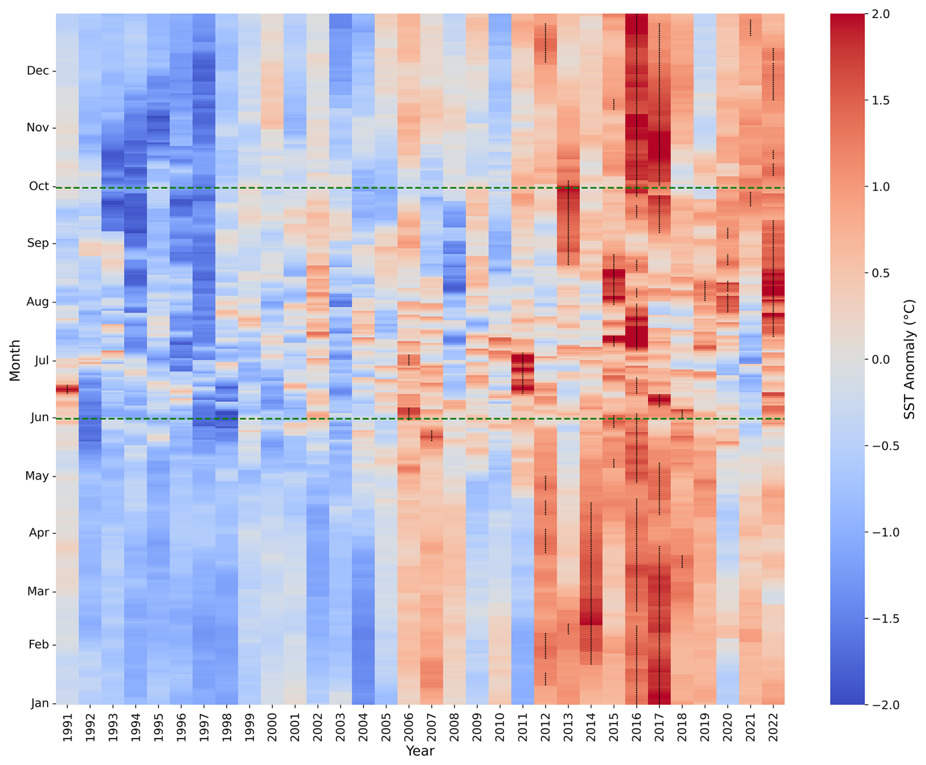
Figure 4 Daily average TOPAZ SST anomaly (°C) relative to the period 1991–2022 for Svalbard West (77–80° N, 5–15° E). Black dots represent when the SST exceeds the 90th percentile, indicating the presence of a MHW. The summer period used for the focus of this study is highlighted by the green dashed line.

3.2.1 MHW Events

Table 1 lists the summer MHW events with a minimum 10 d duration, detected using TOPAZ SST averaged over Svalbard West (77-80° N, 5–15° E), using 1991–2022 as a reference climatology. The sensitivity of MHW detection to the choice of reference period is well documented in literature (e.g., Lien et al., 2024; Smith et al., 2025). To assess this sensitivity, we examined how the MHW metrics for each event in Table 1 changed when using a shorter climatology. When the reference period was restricted to the final 10 years of the reanalysis (2011–2022), the timing of most summer MHWs remained similar. However, a few events (2013, 2022) were divided into two shorter events occurring about a week apart (Table S1 in the Supplement). For events whose timing was largely unaffected by the change in climatology (i.e., those with matching dates under both the 1991–2022 and 2011–2022 baselines), we compared their duration and intensity. Under the shorter climatology, event duration decreased by 5 %–52 % and intensity decreased by 17 %–44 %. The percentage range represents the smallest to largest decrease in mean duration and intensity under the 2011–2022 climatology, relative to the 1991–2022 climatology. The percentage decrease in duration was larger for deep events, compared to shallow events; this pattern, however, was not observed for intensity (Table S1). In summary, shortening the climatology does not substantially alter the timing of most MHWs, but it does reduce their intensity and duration.

Table 1 Summary of summer MHW events in Svalbard West detected using SST averaged over Svalbard West (77–80° N, 5–15° E). The ocean heat content (OHC, 0–300 m) is averaged over Svalbard West (SBW) for the start date of each event.

^a Category II. ^b Category I. ^* Denotes years where MHWs are also detected in winter.

3.2.2 Vertical Extent

Each event is assigned a depth class. Four shallow (≤50 m) and four deep (>50 m) MHWs have been detected (Table 1). The vertical profile for the duration of each MHW event is shown in Figs. 5 and 6. The maximum depth of the events in Table 1 ranged from 10–600 m, with the deepest event found in 2013. Furthermore, the deep events in 2015 and 2016 have a surface event detached from a deep event (Fig. 6). In 2015, the deep event occurs towards the end of the surface event. By contrast, in 2016 the deep event persists for the entire duration of the surface event. In 2015 and 2016, the maximum vertical gap between the surface and deep events was 57 and 85 m, respectively.

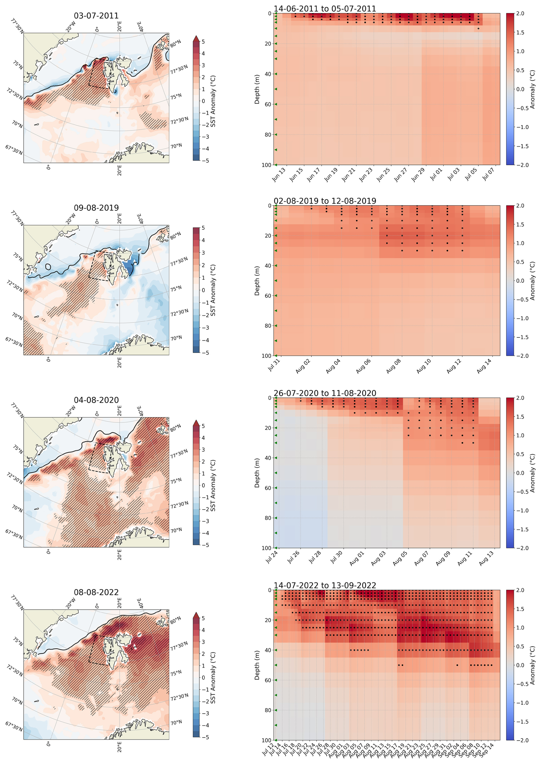
Figure 5 Horizontal (left panel) and vertical (right panel) extent of all detected shallow MHWs. Horizontal extent is shown for the peak date (date of peak intensity – maximum SSTA – for the Svalbard West spatial average) of each MHW. Vertical extent is shown for the entire MHW duration. Hatching represents where the SST or vertical temperature profile exceeds the 90th percentile. The SST anomaly for the peak date and vertical temperature anomaly (°C) are plotted in the background. TOPAZ sea ice edge (sea ice concentration of 15 %) for each date is indicated by the black line in the left panel. MHWs are not detected above the sea ice edge. Green arrows (right panel) represent TOPAZ vertical levels.

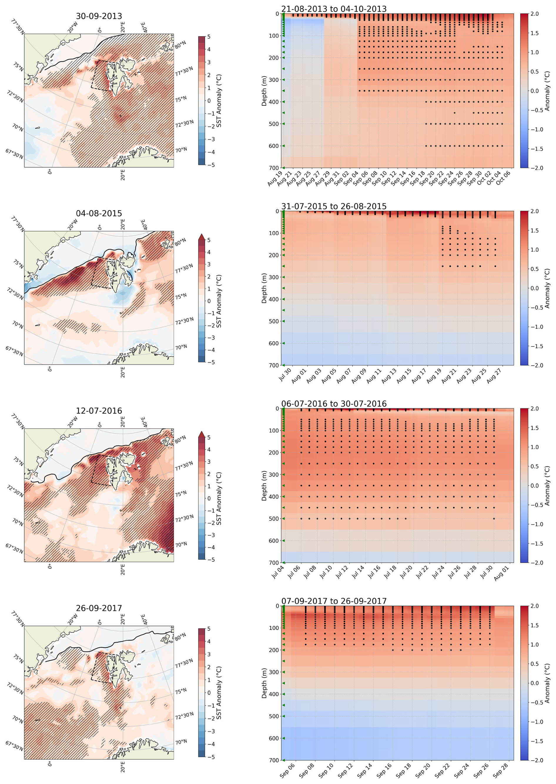
Figure 6 Horizontal (left panel) and vertical (right panel) extent of all detected deep MHWs. Horizontal extent is shown for the peak date (date of peak intensity – maximum SSTA – for the Svalbard West spatial average) of each MHW. Vertical extent is shown for the entire MHW duration. Hatching represents where the SST or vertical temperature profile exceeds the 90th percentile. The SST anomaly for the peak date and vertical temperature anomaly (°C) are plotted in the background. TOPAZ sea ice edge (sea ice concentration of 15 %) for each date is indicated by the black line in the left panel. MHWs are not detected above the sea ice edge. Green arrows (right panel) represent TOPAZ vertical levels.

During the detected surface MHW events, we found temperatures in the ISM mooring to be of similar magnitude to the closest offshore TOPAZ point to the mooring (TP1) at 50 m (not shown). During the detected deep MHW events, temperatures are warmer at the ISM mooring compared to TP1 at 150 m (not shown); thus, TOPAZ underestimates temperatures at this depth. These findings align with the better performance of TOPAZ at shallower depths, as shown in the Methods, Sect. 2.6.

3.2.3 Horizontal Extent

To understand the conditions outside of Svalbard West during each MHW, we determined the horizontal extent at the event peak (date of max intensity) of each MHW in Table 1, within the bounds of 69–82° N, −10° W–35° E (area in left panel, Figs. 5, 6). It is important to note than some events may extend further than this latitude-longitude range. The deep event in 2013 has the largest horizontal extent covering 34.7×10⁵ km² at the event peak. The shallow event in 2019 has the smallest extent covering 8.0×10⁵ km² at the event peak and was largely localised to the Svalbard West region and waters southwest of Svalbard. The shallow event in 2011 was also a local event, reserved largely to the Svalbard West region, covering 8.6×10⁵ km². In the calculation of horizontal extent (km²), spatial continuity was not enforced, and all regions exceeding the 90th percentile were included, even if separated by grid cells below the threshold. Furthermore, MHWs were not analysed north of the TOPAZ sea ice edge (sea ice concentration ≥15 %).

Validation of MHW horizontal extent using DOISST satellite data revealed that the events detected using TOPAZ in Svalbard West were also present in the DOISST data (Fig. S8). Events, however, had a larger extent in the TOPAZ reanalysis compared to satellite data (Figs. 5, 6). Compared to observations over the entire Arctic Ocean (lat > 63° N, all longitudes), TOPAZ exhibits a warm average surface bias of approximately 0.4 °C during summer and underestimates summer sea ice cover (Xie and Bertino, 2024), which may explain the greater horizontal extent observed in the satellite data.

3.3 Drivers of MHW events

To quantify whether the detected MHW events are forced at the surface by air-sea heat fluxes or forced through increased ocean heat transport (OHT), the SHF and OHT for the Svalbard West region have been analysed for each MHW event.

3.3.1 Air-Sea Interaction

The SHF summed over all grid points in Svalbard West for the summer period of each MHW year, exhibits fluctuations both above (red shading) and below (blue shading) the climatological mean (1991–2022, Fig. 7). The climatological mean follows a clear seasonal cycle; positive SHF from June to August means heat input to the ocean from the atmosphere, whilst negative SHF from September to October means heat loss from the ocean to the atmosphere. The overall spread of SHF anomalies during the majority of the events (orange shading) remains mostly within ±1 standard deviation (grey lines). This suggests that while SHF varied during MHW events, it seldom exhibited extreme deviations from historical variability. Nevertheless, in 2015, 2016 and 2020, SHF values show pronounced anomalies at the start date of each MHW, exceeding +1 standard deviation by 0.95 TW (9.5×10¹¹ W), 3.85 TW and 3.25 TW respectively. Furthermore, the long-lasting MHW in 2022 was preceded by positive anomalies more than a month ahead of the start time of the event. Lastly, the SHF anomaly at the start of all events was positive, indicating a net heat gain in the ocean, with the exception of the event in 2017 (event took place in late autumn and a positive SHF anomaly means less heat loss from the ocean than normal).

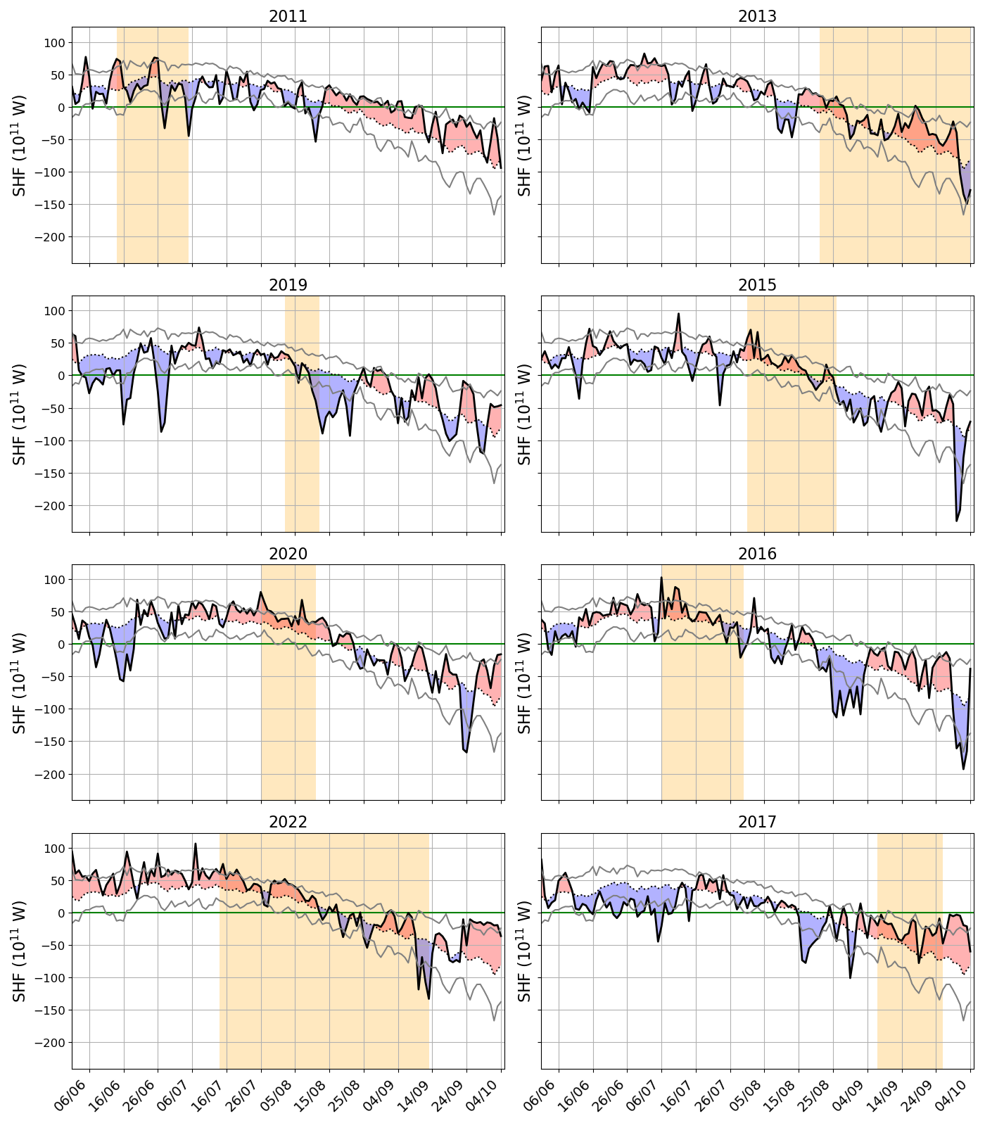
Figure 7 Total surface heat flux (W) for the summer period for each detected shallow (left column) and deep (right column) MHW event in Svalbard West. Red shading represents values above the mean (dotted line, 1991–2022), blue shading represents values below the mean. Orange shading shows the duration of each MHW in Table 1. Grey lines represent ± 1 standard deviation. The zero line (green) is shown.

3.3.2 Ocean Heat Budget

Prior to the individual heat budget analysis for each MHW event, we analysed the 1991–2022 annual mean time series of the ocean heat budget terms (as described in Sect. 2.2). The total cross‐sectional OHT oscillates between approximately 5 and 12 TW. SHF remains within −6 to −12 TW, implying heat loss from the ocean surface, with a positive trend of +0.074 TW yr⁻¹. The residual (difference between OHT and SHF terms) remains clustered around zero, indicating that the sum of advective transport and surface‐flux terms almost account for all of the heat budget variability.

To understand how OHT could have contributed to each MHW, the mean net OHT at the southern, northern and western boundary (OHTs, OHTn, OHTw) of Svalbard West was calculated for the duration of each MHW (Table S2). All events show more heat entering Svalbard West through the southern boundary than leaving through the western and northern boundaries, resulting in an overall positive total OHT and implying a net heat gain in the region (Table S2). For example, for the event in 2022, which had the longest duration, 34 TW entered the region at the southern boundary and a mean of 24 TW exited the region (8 TW through the northern boundary and 16 TW through the western boundary). Thus, the inflow exceeded the outflow by 10 TW, resulting in a net heat gain during the 2022 event.

As we are interested in understanding how the extreme situations happened, we compared the mean net OHT during the events with the respective climatology (1991–2022). Anomalous OHT for each boundary are shown in Fig. 8a. All events show a positive anomaly at the southern boundary (Fig. 8a), implying anomalous heat input into the region. Furthermore, the majority of events show a negative anomaly at the northern and western boundaries, implying more heat leaving than normal. The exceptions are the shallow events in 2019 and 2020, which have a positive anomaly at the western boundary, implying less heat leaving at the western boundary. Furthermore, the event in 2022 has a positive anomaly at the northern boundary, implying less heat leaving at the northern boundary during this event. Less heat leaving at the western/northern boundary, in addition to higher OHT than normal across the southern boundary, could explain the high positive total OHT anomalies shown for 2019, 2020, and 2022 in Fig. 8b.

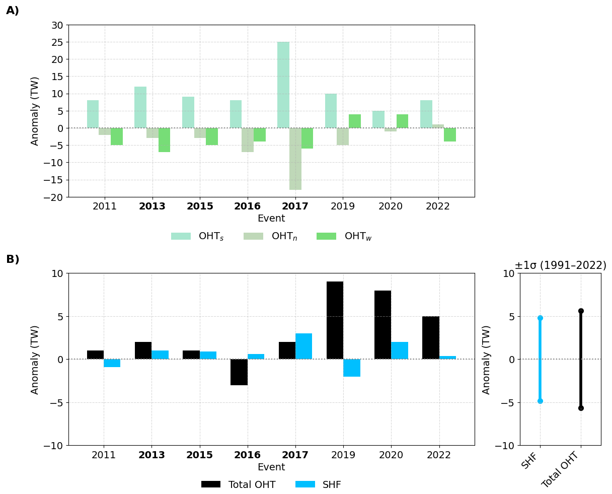
Figure 8 (a) Mean ocean heat transport (OHT) anomalies at the southern (OHTs), northern (OHTn) and western boundary (OHTw) of Svalbard West during each event. Deep events are marked in bold. (b) Mean anomalies of the budget terms (total OHT and SHF) for the duration of each MHW event in Svalbard West (left panel) and their standard deviation (right panel). The standard deviation is based on daily values from Svalbard West for all summers (JJAS) from 1991–2022. Bold: deep events. Plain: Shallow events. Note that in both (a) and (b) the x-axis shows individual events not a continuous time axis.

Focussing further on the total OHT anomaly for the duration of each event, the largest net heat gain happened in 2019 and 2020 with anomalies of 8–9 TW during the events (Fig. 8b). OHT anomalies are considerably higher in more recent events (2019, 2020 and 2022) compared to those in 2011–2017, with anomalies clearly outside +1 standard deviation in 2019 and 2020 (Fig. 8b). Compared to SHF, except for events in 2016 and 2017 (deep events), the analysis shows that OHT anomalies exceed SHF anomalies (Fig. 8b) and SHF anomalies during the events do not exceed ±1 standard deviation, consistent with the results in Fig. 7. In 2016, the event was characterised by a negative OHT anomaly, implying anomalous net heat export from the region. It is important to note that during the 2016 event an 8 TW anomaly was apparent at the southern boundary (Fig. 8a), therefore, despite the overall negative OHT anomaly, this event was not driven by SHF alone. The results above indicate that OHT is the dominant driver of most prolonged events over 2011–2022.

4 Discussion

Marine heatwaves (MHWs) were described around Svalbard from 1991–2022 using a physical reanalysis for the North Atlantic and Arctic region – based on TOPAZ. Our analysis indicated that the duration and frequency of MHWs have increased around Svalbard in the last decade of the reanalysis, with less change observed in the intensity of events. Focusing on summer events (June–September) in Svalbard West that lasted longer than 10 d, we identified the presence of four shallow (≤50 m) and four deep (>50 m) MHWs. Through heat budget analysis, overall, we found a greater contribution of ocean heat transport (OHT) than surface heat flux (SHF) in driving MHW events.

4.1 MHW Definition

In this study, we applied methods from Hobday et al. (2016), whereby MHWs are detected when the daily sea surface temperature (SST) exceeds the 90th percentile for at least 5 consecutive days, with no more than two below-threshold days. Additionally, we used a fixed baseline of 32 years (1991–2022) to calculate the percentile. The same approach is used by Mohamed et al. (2022), when studying MHWs in the Barents Sea. A fixed baseline provides a stable reference for detecting long-term SST trends in MHW studies. While a fixed baseline is commonly used, some advocate for a shifting baseline to exclude the effects of climate change (Jacox, 2019). Hobday et al. (2018) and Bashiri et al. (2024), however, have advised against using a shifting baseline as updating the baseline climatology over time can change how past events are classified. Eisbrenner et al. (2024), compared a shifting baseline approach to a fixed baseline approach to study MHWs in the Barents Sea, and found that using a shifting baseline approach decreased the intensity of MHW events compared to a fixed baseline case.

Baseline length can also affect MHW metrics. In our study, when the baseline was adjusted to the last 10 years of the reanalysis (2011–2022), the timing of most summer MHW events remained largely unchanged (Table S1). However, a decrease in duration and intensity was found when the baseline was shortened. Lien et al. (2024) also found a general trend of decreasing average intensity with decreasing length of the baseline. In addition, we found that the decrease in duration was larger for deep events compared to shallow events. The above differences in MHW characteristics caused by changing the baseline highlights the need, as emphasised by Amaya et al. (2023), for the definition of MHWs to be standardised.

The MHW research community also debates whether temperature data should be detrended prior to MHW detection. Detrending, often by removing a linear trend (Smith et al., 2025), aims to separate MHWs from the long-term warming signal (Jacox, 2019) and is used in several global and Arctic studies (Jacox et al., 2020; Xu et al., 2022; Golubeva et al., 2021). In the Arctic, warming is not necessarily linear and is strongly influenced by natural variability, including decadal thermohaline anomalies in the North Atlantic-Arctic region (Årthun et al., 2017; Passos et al., 2024), that modulate Atlantic inflows to the Nordic Seas on multi-year to decadal scales (Chafik et al., 2025). Such variability might explain part of the decadal variability in MHW frequency for the northern Nordic Seas (Fig. S7). Given these complexities, we argue that using raw (non-detrended) temperature data is more appropriate for Arctic MHW detection.

4.2 Areas of high MHW activity and long-term trends

We find regional differences in MHW activity across the Svalbard Archipelago and its surrounding seas (Fig. 3). The highest MHW intensity is located at water mass fronts. For example, high MHW intensity is found in the location of the Polar Front, southeast of Svalbard (description of the Polar Front is given in Mohamed et al., 2022; Barton et al., 2018). The above could be attributed to the high variability of SST in this region (Mohamed et al., 2022). High MHW intensity, including high frequency and duration in the last decade, is also found southwest of Svalbard along the Mohn Ridge, in the pathway of the NwAFC (Fig. 1) in the Arctic Front. A high number of MHWs at the Mohn Ridge could be attributed to high seasonal and interrannual temperature variability in the region or due to strong temperature gradients, associated with the interaction of warm and saline Atlantic Water with colder and fresher Arctic Water (Akhtyamova and Travkin, 2023). Lastly, lateral exchanges, such as eddies across the front, could trigger MHW events by bringing warmer water into a normally colder water region.

Large changes in MHW frequency and duration is found on the West Spitsbergen Shelf (Fig. 3). One reason for this could be the shoaling of Atlantic Water (AW) associated with the Atlantification seen in western Svalbard fjords and north and west of Svalbard. Atlantification refers to the increased influence of AW in the Arctic driven by recent warming of the AW inflow (Årthun et al., 2012). AW has been observed higher in the water column and along shallower isobaths in Isfjorden (Skogseth et al., 2020) and Kongsfjorden (Tverberg et al., 2019, for location see Fig. 1). North of Svalbard, Atlantification can be observed in the eastern Eurasian Basin, as evidenced by a weakening of the halocline and a shoaling of the intermediate-depth AW layer (Polyakov et al., 2017). Furthermore, on the shelf southwest of Svalbard, Strzelewicz et al. (2022) reported a 8 % yr⁻¹ increase in the volume fraction of AW. Since AW inflow along the West Spitsbergen shelf is warming (Beszczynska-Möller et al., 2012), a shoaling and increased presence of warming AW can lead to higher MHW frequency and duration.

The variability of AW temperature west of Svalbard has been shown to be associated with the strength of the Greenland Sea Gyre (GSG) circulation influenced by the anomalous wind stress curl over the Nordic Seas (Chatterjee et al., 2018). A stronger GSG circulation increases the AW flow speed west of Svalbard, leading to increased oceanic heat content and higher AW temperature therein (Chatterjee et al., 2018). Thus, increased AW temperature driven by strong GSG circulation may also be responsible for the increase in MHW events in Svalbard West.

4.3 Spatial extent of the MHW events

MHWs in Svalbard West exhibited substantial spatial variability, ranging from local events confined to the archipelago to widespread events extending beyond Svalbard, and from shallow surface anomalies to depths reaching up to 600 m (Figs. 5, 6). Previous studies, for example, Zhang et al. (2023), define the vertical structure of MHWs by averaging temperature anomalies from in-situ profiles over the event duration. Instead of averaging, we examined the day-to-day vertical progression of each MHW by identifying the depth levels exceeding the 90th percentile on each day of the event. Understanding the horizontal and vertical extent of individual MHW events, represents a novel set of criteria that provide a valuable framework for future MHW characterisation.

As noted in Sect. 2.1, since MHWs in this study are detected using SST, our methods overlook events that lack a surface expression. Global studies have shown that a significant proportion of MHWs occur in the subsurface without leaving a detectable SST signature (Sun et al., 2023); this therefore represents an important limitation of our study. Studies on subsurface MHWs in the Arctic are limited. Lien et al. (2024) detected bottom MHWs in the Barents Sea, which were shown to have a longer duration than surface events. Bottom MHWs could thus imply a greater potential for ecosystem damage, underscoring the need for future studies to consider events that do not exhibit a surface signal. Malan et al. (2025) have proposed a classification scheme for subsurface MHW events that distinguishes between mixed‐layer, deep, thermocline, full‐depth, submerged and benthic MHWs. Applying such detailed classification to describe the vertical extent of events can improve our understanding of ecosystem impacts, by helping to identify which species and habitats are most likely to be affected.

4.4 Drivers of the MHW events

Our results show that advective heating is the primary driver of most summer MHWs in Svalbard West, with positive OHT anomalies exceeding SHF anomalies in all but two events (Fig. 8b). Poleward heat transport by boundary currents can drive subsurface warming, and through vertical mixing can elevate SSTs and produce a MHW (Holbrook et al., 2019). During all the events identified in this study, mean OHT into Svalbard West across its southern boundary exceeded the combined outflow through the northern and western boundaries (Table S2). This net heat gain can elevate temperature anomalies and ultimately drive MHW development. Furthermore, all events show a positive anomaly at the southern boundary (Fig. 8a), implying anomalous heat input into the region that contributes to the development of MHWs. In contrast to our results, Arctic-wide assessments identify surface heat fluxes as the dominant driver of summer MHWs (Richaud et al., 2024), with lateral advection generally considered as a secondary driver. However, Richaud et al. (2024) also highlighted that OHT can become the leading contributor to MHWs at the main Arctic gateways, where heat advection is particularly pronounced. The importance of advection in driving MHWs in our region is further supported by Lien et al. (2024), who found that enhanced AW transport contributed to the onset of the 2016 Barents Sea MHW.

Despite the leading role of OHT in driving MHWs in Svalbard West, atmospheric heating also contributes to their development. Positive mean SHF anomalies are found for all but two events (Fig. 8b), indicating anomalous heat input from the atmosphere during the majority of the MHWs. Negative anomalies are shown for the 2011 and 2019 MHW, which also display the smallest horizontal extent compared to the other events. Positive SHF anomalies are also found at the start date of each MHW, indicating enhanced heat input for events initiated in summer and reduced heat loss for those initiated in late summer/early autumn (Fig. 7). For the events with a positive mean SHF (five out of eight events, Table S2), atmospheric heating contributes to a net heat input at the ocean surface, which directly warms the upper ocean. Anomalous atmospheric heating can trigger or enhance SST anomalies, contributing to MHW development. SST anomalies driven by an anomalous SHF can, through vertical mixing and entrainment, lead to positive subsurface temperature anomalies and contribute to driving deep MHW events (Richaud et al., 2024). The atmospheric heating effect is further intensified by oceanic heat advection, as described above. In previous studies, an interplay between the ocean and atmosphere has proven to be important for the onset of MHW events, for example in the Barents Sea (Eisbrenner et al., 2024). In addition, the 2016 event identified in this present study has been linked to atmospheric forcing: Mohamed et al. (2022) suggested that warm air temperature anomalies of approximately ≥2 °C played a key role in its development over the Barents Sea, while Lien et al. (2024) reported that reduced heat loss to the atmosphere during the winter of 2015–2016 contributed to its onset.

5 Conclusions

In conclusion, an increase in marine heatwaves (MHWs) is evident in Svalbard West and around the Svalbard Archipelago in the last decade. Events are shown to be both shallow/deep and local/widespread reaching depths greater than 50 m and extending from the Svalbard Archipelago to the Barents Sea. Our findings indicate that compared to air-sea heat fluxes, heat advection from ocean currents plays a greater role in driving MHWs in Svalbard West. Identifying individual MHWs by their horizontal and vertical extent, as achieved by this study, is a useful metric that could be applied to future MHW studies to determine which ecosystems will be impacted by individual events. This study has demonstrated that ocean reanalysis, such as TOPAZ, are a useful tool for analysing the spatial extent and drivers of MHW events. As MHW research advances, greater emphasis on their ecological consequences is essential, particularly due to the fact that, driven by the climate change signal, their frequency and duration are projected to increase.