Observation-based quantification of physical processes that impact sea level

This study provides observationally based estimates of the contributions to sea level rise from individual physical oceanographic processes. The kinematic equation for sea level evolution is used to calculate the spatial distribution of the evolution of sea level rise, and its global integral. Results are separated into impacts from boundary mass fluxes and from non-Boussinesq steric effects. The non-Boussinesq steric effect itself is further decomposed into contributions from boundary buoyancy fluxes and interior buoyancy changes driven by mixing processes. It is neither the intention nor currently possible to close the global mean sea level (GMSL) budget using this approach. Instead, the results quantify the magnitude and uncertainty of the physical oceanographic processes and their relative importance in shaping GMSL rise. This allows for a comparison of the impact on GMSL by single processes or parameterizations. Results indicate large uncertainties associated with boundary heat, mass, and freshwater fluxes and highlight the importance of ocean mixing for GMSL rise. Additionally, GMSL rise is substantially affected by how shortwave radiation is redistributed with depth and by the choice of neutral physics calculation method. This study also finds that nonlinear thermal expansion is offset by mixing-induced densification, and that both processes strongly influence sea level as consequences of the nonlinear equation of state. Many of the results are relevant for observationally based calculations and for modelers making decisions about which methods or parameterizations to use. Understanding the impact of these processes on GMSL rise, and how they change in a transient ocean and climate system, is important because these choices influence projections of future sea level rise, which inform policy decisions.

1 Introduction

Since 1850, human-induced warming has increased global surface temperatures by approximately 1.1 °C (Eyring et al., 2023). About 89 % of this anthropogenic heat has been absorbed by the ocean (von Schuckmann et al., 2020), leading to significant ocean warming (Li et al., 2023), thermal expansion and associated sea level rise (Horwath et al., 2022). Approximately 4 % of the warming since the pre-industrial era has contributed to the melting of glaciers and ice sheets, further elevating global sea level. The remaining heat has been stored in land (6 %) and the atmosphere (1 %).

Global mean sea level (GMSL) rise is estimated using satellite altimetry (Ablain et al., 2017; Hamlington et al., 2024) and tide gauges (Jevrejeva et al., 2006; Hamlington et al., 2022). Since 1901, GMSL has risen by approximately 21 cm (Fox-Kemper et al., 2023). Sea level rise has accelerated from 1.35 mm yr⁻¹ between 1901 and 1990 to 3.7 mm yr⁻¹ between 2006 and 2018 (Chapter 9, Table 9.5, Fox-Kemper et al. (2023), Nerem et al., 2018), and it is projected to accelerate further (Nerem et al., 2022). Currently, the main contributions to sea level rise are thermal expansion (39 %, 1.4 mm yr⁻¹) and the combined contributions from glaciers and ice sheets (45 %, 1.6 mm yr⁻¹).

The GMSL rise budget can be closed by summing contributions from steric and barystatic changes. Steric sea level change is obtained by integrating global ocean temperature and salinity observations (Pattullo et al., 1955; Antonov et al., 2002) and accounted for roughly 34 % of GMSL rise between 1900 and 2018 (Frederikse et al., 2020). Barystatic change, derived from satellite observations of mass fluxes from glaciers, ice sheets, and terrestrial water storage (Shepherd et al., 2018; Fasullo and Nerem, 2018), contributed approximately 66 % of GMSL rise over the same period (Frederikse et al., 2020). These “top-down” approaches have enabled the closure of GMSL budgets within statistical uncertainty (Moore et al., 2011; Horwath et al., 2022; Frederikse et al., 2020; Church et al., 2011; Ludwigsen et al., 2024).

Instead of a top-down approach, this study uses a “bottom-up” strategy, estimating GMSL as the sum of contributions from individual physical oceanographic processes that alter ocean density and volume. The kinematic equation for sea level evolution is used to calculate the impacts of boundary mass fluxes and non-Boussinesq steric effects on sea level rise. Non-Boussinesq steric effects are further decomposed into contributions from boundary freshwater, heat, and salt fluxes, and from interior diffusive and advective fluxes generated by oceanic turbulent eddies. This bottom-up approach was previously applied by Griffies and Greatbatch (2012) within numerical models, successfully closing the model's GMSL budget.

This study uses observation-based datasets instead of numerical models to quantify sea level changes caused by physical oceanographic processes. This allows for an assessment of how uncertainties in observations or parameterizations influence GMSL calculations and how these compare to observed GMSL rise rates. Rates of sea level rise are calculated using annual-mean observational hydrography, representing annual-mean changes. Results are presented as spatially varying maps of local sea level changes and as their global integrals to estimate GMSL rise. However, due to large uncertainties in observational products, it is neither intended nor possible at this stage to observationally close the GMSL budget using this approach. This highlights the lack of observational constraints on air–sea interactions, mass fluxes, and mixing, as well as incomplete understanding and representation of fundamental physical mechanisms underlying GMSL budgets.

Specifically, this study examines the impacts of variations in heat, mass and freshwater flux products, mixing strength parameterizations, neutral physics, shortwave radiation depth penetration parameterizations, and eddy stirring parameterizations. All of these processes substantially influence GMSL rise, with first-order impacts of the order of millimeters per year. These results are relevant for numerical ocean and climate models, as modelers must make decisions on how to represent these processes, which in turn affect projections of future sea level rise. Quantifying the impact of different parameterizations on GMSL in numerical ocean models is difficult due to the complexity and expense of reprogramming and rerunning the model and because of difficulties to isolate the impact of a single change.

1.1 Nonlinear thermal expansion and densification upon mixing

This study also investigates whether “densification upon mixing” can prevent the ocean from ever expanding due to warming (Schanze and Schmitt, 2013). Even without anthropogenic warming, an ocean with a net-zero global heat flux would still expand, causing sea level rise. This occurs because the thermal expansion coefficient α varies with temperature (and to a lesser extent, salinity and pressure). Warmer water expands more than colder water contracts.

Since ocean warming primarily occurs in low latitudes over warm waters and cooling occurs at higher latitudes over colder waters, warming drives greater expansion than cooling drives contraction. Globally integrated, this produces a net ocean volume increase that contributes to GMSL (Griffies and Greatbatch, 2012; Schanze and Schmitt, 2013). This study refers to this process as “nonlinear thermal expansion” as it occurs only due to nonlinearity of the equation of state, distinct from the thermal expansion caused by a net heat flux into the ocean. It should not be confused with the thermobaric effect or thermobaricity, which arises from variations in the thermal expansion coefficient with pressure.

Densification upon mixing can reduce sea level (Gille, 2004; Jayne et al., 2004) and thereby counteract nonlinear thermal expansion. This occurs when two water parcels mix, and the resulting mean density is greater than the average of the original densities due to the nonlinear equation of state. This process, also known as cabbeling (Witte, 1902; Foster, 1972; McDougall, 1987b), contracts water volume and lowers sea level. As first suggested by McDougall and Garrett (1992), densification upon mixing opposes nonlinear thermal expansion, potentially preventing unbounded ocean expansion. While Schanze and Schmitt (2013) estimated the magnitude of densification upon mixing using air–sea heat fluxes, it has not been verified from independent sources, that this is of the same order as nonlinear thermal expansion. This study addresses that gap.

This paper is organized as follows. Section 2 derives the equations governing physical oceanographic processes influencing the GMSL budget and discusses assumptions and processes not covered. Section 3 describes the datasets used. Section 4 presents results for nonlinear thermal expansion (Sect. 4.3), densification upon mixing (Sect. 4.6), shortwave radiation (Sect. 4.4), and stirring (Sect. 4.7), among others. Section 5 provides a summary, discussion of caveats, and implications, followed by a brief conclusion in Sect. 6.

2 Theory

Sea level changes due to adding or redistributing mass, and due to changes in ocean density (Gill and Niller, 1973). Following Griffies and Greatbatch (2012) (their Eq. 1), these effects are described using the kinematic equation for sea level evolution:

$$\begin{array}{}\text{(1)}& \underset{\begin{array}{c}\text{sea level}\\ \text{evolution}\end{array}}{\underbrace{{\displaystyle \frac{\partial \mathit{\eta }}{\partial t}}}}=\underset{\begin{array}{c}\text{boundary}\\ \text{mass flux}\end{array}}{\underbrace{{\displaystyle \frac{Q_{\text{mass}}}{\mathit{\rho }(z=\mathit{\eta })}}}}\underset{\begin{array}{c}\text{dynamic}\\ \text{changes}\end{array}}{\underbrace{-\mathrm{\nabla }\cdot \underset{-H}{\overset{\mathit{\eta }}{\int }}\mathbf{u}\mathrm{d}z}}\underset{\begin{array}{c}\text{Non-Boussinesq}\\ \text{steric}\end{array}}{\underbrace{-\underset{-H}{\overset{\mathit{\eta }}{\int }}{\displaystyle \frac{\mathrm{1}}{\mathit{\rho }}}{\displaystyle \frac{\mathrm{d}\mathit{\rho }}{\mathrm{d}t}}}}.\end{array}$$

Here both integrals are from the ocean bottom height (−H) to the ocean surface height (η). Sea level evolution (l.h.s. of Eq. 1) is evaluated locally for a vertical water column by taking the sum of (i) the boundary mass fluxes, (ii) the redistribution of ocean volume by ocean currents (dynamic changes), and (iii) Non-Boussinesq steric changes. The latter is the expansion or contraction of seawater volume due to changes in sea water density. Changes in sea water density are due to small-scale or mesoscale mixing processes, due to air–sea heat, mass and freshwater fluxes, or due to geothermal heating (see Appendix A for details). Equation (1) is derived under the assumptions that the ocean bottom does not move, the ocean surface area is constant and that the gravitational acceleration is constant (Griffies and Greatbatch, 2012). Processes not covered are the inverse barometer effect, the tidal sea surface elevations and joule heating (Griffies and Greatbatch, 2012).

This study presents both maps of the spatial structure of sea level evolution, as well as the global integral of these maps that provide the net GMSL changes. The spatial structure is given by applying Eq. (1) to a vertical water column, while its impact on GMSL rise $\partial \stackrel{\mathrm{‾}}{\mathit{\eta }}/\partial t$ is obtained by integrating those results globally, using:

$$\begin{array}{}\text{(2)}& {\displaystyle \frac{\partial \stackrel{\mathrm{‾}}{\mathit{\eta }}}{\partial t}}={\displaystyle \frac{\mathrm{1}}{\mathcal{A}}}\underset{\text{globe}}{\int }{\displaystyle \frac{\partial \mathit{\eta }}{\partial t}}\mathrm{d}A,\text{with}\mathcal{A}=\underset{\text{globe}}{\int }\mathrm{d}A.\end{array}$$

Under a no-flux boundary condition, the term “dynamic changes” in Eq. (1) vanishes (second term, r.h.s.). Therefore, ocean currents have no net effect on GMSL rise and instead only redistribute volume.

In the remainder of this section the sea level calculations for the boundary mass fluxes (Sect. 2.1) and redistribution of ocean volume by ocean currents (Sect. 2.4), are specified. This study presents sea level calculations of the non-Boussinesq steric changes due to diffusive salt and heat fluxes (Sect. 2.3), skew fluxes of salt and heat (Sect. 2.4), and by the combination of direct and indirect boundary fluxes of salt and heat (Sect. 2.2). The details of most derivations are moved to the appendices. Derivations rely heavily on (Griffies and Greatbatch, 2012) and (Groeskamp et al., 2019b).

2.1 Sea level change due to a boundary mass fluxes

At the ocean boundaries, the ocean mass flux Q_mass ($\mathrm{kg}{\mathrm{s}}^{-\mathrm{1}}{\mathrm{m}}^{-\mathrm{2}}$) is defined as positive into the ocean and given by:

$$\begin{array}{}\text{(3)}& Q_{\text{mass}}=P-E+R+I+A_{\mathrm{e}},\end{array}$$

where P is precipitation (positive into the ocean), E is evaporation (positive out of the ocean), R is runoff from rivers (positive into the ocean), I is runoff from land ice melt (positive into the ocean), and A_e is the aeolian deposition of salt (positive into the ocean). These mass fluxes can enter the ocean by crossing the ocean surface (E, P, and A_e), laterally (R) or from both directions (I). Inserting Eq. (3) into the first term on the r.h.s. of Eq. (1) leaves:

$$\begin{array}{}\text{(4)}& {\left.{\displaystyle \frac{\partial \mathit{\eta }}{\partial t}}\right|}_{\text{mass}}={\displaystyle \frac{Q_{\text{mass}}}{\mathit{\rho }\left(\mathit{\eta }\right)}}={\displaystyle \frac{\mathrm{1}}{\mathit{\rho }\left(\mathit{\eta }\right)}}\left(P-E+R+I+A_{\mathrm{e}}\right).\end{array}$$

When Eq. (4) is integrated globally, even for a net-zero global mean mass flux, there can still be a net contribution to GMSL rise. This is because the impact of the mass flux on volume is weighted by the sea surface density ρ(η) (Sect. 4.1). This effect is conceptually similar to the impact of a changing thermal expansion coefficient for a net-zero global heat-flux as previously mentioned in Sect. 1 and detailed in Appendix B.

2.2 Sea level change due to boundary heat, salt and freshwater fluxes

Boundary mass fluxes into the ocean (e.g., evaporation, precipitation, ice melt), as well as direct sources of heat and salt, all impact sea level. The impact of such boundary fluxes on sea level rise can be expressed as:

$$\begin{array}{}\text{(5)}& {\left.{\displaystyle \frac{\partial \mathit{\eta }}{\partial t}}\right|}_{\text{boundary}}=-\underset{-H}{\overset{\mathit{\eta }}{\int }}{\displaystyle \frac{\mathrm{1}}{\mathit{\rho }}}\left(F_{\text{mass}}^{\mathit{\rho }}+F_{\text{surface}}^{\mathit{\rho }}+F_{\text{geo}}^{\mathit{\rho }}+F_{\text{swr}}^{\mathit{\rho }}\right)\mathrm{d}z.\end{array}$$

The details for deriving Eq. (5) can be found in Appendix B. The term $F_{\text{mass}}^{\mathit{\rho }}$ ($\mathrm{kg}{\mathrm{m}}^{-\mathrm{3}}{\mathrm{s}}^{-\mathrm{1}}$) represents the changes in local ocean density due to ocean mass fluxes (Q_mass), primarily through alterations of local salinity. Here $F_{\text{surface}}^{\mathit{\rho }}$ ($\mathrm{kg}{\mathrm{m}}^{-\mathrm{3}}{\mathrm{s}}^{-\mathrm{1}}$) captures the impact on density by direct sources of salinity and heat at the surface of the ocean. Surface salt fluxes (e.g., due to sea ice melt or sea spray) are not considered in this analysis, because they are unknown or negligible. Surface heat fluxes are longwave radiation as well as latent and sensible heat fluxes. Shortwave radiation (SWR) enters the ocean surface and can penetrate to deeper layers depending on the clarity of the water (Paulson and Simpson, 1977). The impact of shortwave radiation on ocean density is represented by the term $F_{\text{swr}}^{\mathit{\rho }}$ ($\mathrm{kg}{\mathrm{m}}^{-\mathrm{3}}{\mathrm{s}}^{-\mathrm{1}}$) and is a term separate from $F_{\text{surface}}^{\mathit{\rho }}$. Geothermal heating at the sea floor is given by $F_{\text{geo}}^{\mathit{\rho }}$ and has a small impact on ocean density (de Lavergne et al., 2015).

2.3 Sea level change due to diffusive fluxes

In this section an expression is derived for the impact of diffusive mixing on density and sea level. Mixing is split into a contribution from mesoscale and small-scale processes (Fox-Kemper et al., 2019). Small-scale mixing is due to eddies on the order of a meter that are most commonly associated with breaking internal waves and boundary-layer processes (MacKinnon et al., 2013; Large et al., 1994). This mixing is represented by a vertical turbulent diffusivity D acting on vertical tracer gradients (McDougall et al., 2014). The magnitude of the vertical eddy diffusivity is typically of 𝒪 (${\mathrm{10}}^{-\mathrm{5}}-{\mathrm{10}}^{-\mathrm{3}}{\mathrm{m}}^{\mathrm{2}}{\mathrm{s}}^{-\mathrm{1}}$) (Polzin et al., 1997; Whalen et al., 2012; de Lavergne et al., 2020). Mesoscale eddies of 𝒪 (20–200 km) that stir tracers along neutral directions are parameterized by isoneutral eddy diffusivity K_N acting on tracer gradient along a neutral direction ∇_NC (Redi, 1982; Griffies, 1998; McDougall et al., 2014). When influenced by the geometric constraints of the surface boundary, mesoscale stirring leads to horizontally oriented mixing across outcropped density surfaces (Tandon and Garrett, 1997; Treguier et al., 1997; Ferrari et al., 2008), which is parameterized by a horizontal diffusivity K_H acting on horizontal tracer gradient ∇_HC. The magnitude for K_N and K_H is typically 𝒪 (${\mathrm{10}}^{\mathrm{1}}-{\mathrm{10}}^{\mathrm{3}}{\mathrm{m}}^{\mathrm{2}}{\mathrm{s}}^{-\mathrm{1}}$) (Abernathey and Marshall, 2013; Klocker and Abernathey, 2013; Cole et al., 2015; Roach et al., 2018; Groeskamp et al., 2017, 2020; Sévellec et al., 2022; Kusters et al., 2024).

The above mixing directions are represented by a symmetric positive-definite kinematic diffusivity tensor K (m² s⁻¹) that contains the contributions of the mesoscale neutral and horizontal diffusion, and small-scale isotropic diffusion. This leads to the following expression for the impact of diffusive mixing on density and sea level, for which the details are provided in Appendix C:

$$\begin{array}{}\text{(6)}& \begin{array}{rl}{\displaystyle }& {\displaystyle }{\left.{\displaystyle \frac{\partial \mathit{\eta }}{\partial t}}\right|}_{\text{diffusion}}\approx \\ {\displaystyle }& {\displaystyle }-\underset{\text{Redistribution}}{\underbrace{{\mathrm{\nabla }}_{\mathrm{H}}\cdot \underset{-H}{\overset{\mathit{\eta }}{\int }}{\mathbf{R}}^{\text{hor}}\mathrm{d}z}}+\underset{\text{diffusion–boundary interaction}}{\underbrace{{\mathbf{R}}^{\text{hor}}\left(\mathit{\eta }\right)\cdot {\mathrm{\nabla }}_{\mathrm{H}}\mathit{\eta }-{\mathbf{R}}^{\text{hor}}(-H)\cdot {\mathrm{\nabla }}_{\mathrm{H}}(-H)}}\\ {\displaystyle }& {\displaystyle }+\underset{\text{diffusion–density interaction}}{\underbrace{\underset{-H}{\overset{\mathit{\eta }}{\int }}{K}_{\mathrm{H}}^{-\mathrm{1}}{\left|{\mathbf{R}}^{\text{hor}}\right|}^{\mathrm{2}}\mathrm{d}z+\underset{-H}{\overset{\mathit{\eta }}{\int }}{D}^{-\mathrm{1}}{\left|{\mathbf{R}}^{\text{ver}}\right|}^{\mathrm{2}}\mathrm{d}z-\underset{-H}{\overset{\mathit{\eta }}{\int }}\mathit{\rho }g\mathit{\kappa }\mathbf{k}\cdot {\mathbf{R}}^{\text{ver}}\mathrm{d}z}}\\ {\displaystyle }& {\displaystyle }+\underset{\text{Cabbeling and Thermobaricity}}{\underbrace{\underset{-H}{\overset{\mathit{\eta }}{\int }}{P}_{T_{\mathrm{b}}}^{\text{ntr}}+P_{C_{\mathrm{b}}}^{\text{ntr}}+P_{C_{\mathrm{b}}}^{\text{hor}}+P_{T_{\mathrm{b}}}^{\text{ver}}+P_{C_{\mathrm{b}}}^{\text{ver}}\mathrm{d}z}},\end{array}\end{array}$$

where the following definitions (see Appendix C) apply:

$$\begin{array}{}\text{(7)}& {\displaystyle }& {\displaystyle }\mathbf{R}=-\mathit{\alpha }\mathbf{K}\cdot \mathrm{\nabla }\mathrm{\Theta }+\mathit{\beta }\mathbf{K}\cdot \mathrm{\nabla }{S}_{\mathrm{A}},\text{(8)}& {\displaystyle }& {\displaystyle }\mathrm{P}=\mathrm{\nabla }\mathit{\alpha }\cdot \left(\mathbf{K}\cdot \mathrm{\nabla }\mathrm{\Theta }\right)-\mathrm{\nabla }\mathit{\beta }\cdot \left(\mathbf{K}\cdot \mathrm{\nabla }{S}_{\mathrm{A}}\right).\end{array}$$

Here Θ is Conservative Temperature (McDougall, 2003; Graham and McDougall, 2013), S_A is Absolute Salinity (McDougall et al., 2012; Millero et al., 2008). Further, R^ntr, R^hor, and R^ver (m s⁻¹) are the components of R for the three different mixing direction “neutral”, “horizontal” and “vertical”, respectively. Then P^ntr, P^hor, and P^ver are the components of P (s⁻¹) for the three different mixing direction. For the neutral direction α∇_NΘ=β∇_NS_A, and thus R^ntr=0. The first term on the r.h.s. of Eq. (6) named “redistribution” turns out to be large, but also globally integrates to zero due to the divergence operator. By explicitly writing Eq. (6) in a form that contains this redistribution term, this creates the term named “diffusion-density interaction” that can be interpreted as the interaction between diffusion and density gradients. This term will turn out to be small, such that it is advantageous to write Eq. (6) in this form, as it allows for neglecting the global integration of the redistribution term and the diffusion-density interaction term. The term named “Production” is the interaction between diffusion and the nonlinear equation of state. This term includes the terms causing densification upon mixing, cabbeling and the thermobaric terms, as specified in Appendix C1. Thermobaricity can in fact lead to both an increase and decrease in density, but its impact on density is generally an order of magnitude smaller than that due to cabbeling (Klocker and McDougall, 2010; Groeskamp et al., 2016). Although cabbeling and thermobaricity are names specifically referring to neutral mixing (McDougall, 1987b), effects of the nonlinear equation of state that change density due to mixing of Θ and S_A, are not limited to the neutral direction. The same abbreviations for the mixing directions as before are used for the impact of cabbeling ($P_{C_{\mathrm{b}}}^{\text{ntr}},P_{C_{\mathrm{b}}}^{\text{hor}},P_{C_{\mathrm{b}}}^{\text{ver}}$) and thermobaricity ($P_{T_{\mathrm{b}}}^{\text{ntr}},P_{T_{\mathrm{b}}}^{\text{hor}},P_{T_{\mathrm{b}}}^{\text{ver}}$), due to the different mixing processes.

2.4 Sea level change due to ocean dynamics and eddy-induced transport

The convergence of the vertically integrated horizontal ocean velocity u can lead to redistribution of volume and thus a local impact on sea level, while its global integral is zero under the assumption that there is no velocity through the boundaries. The velocity u will be approximated as the sum of the geostrophic velocity u_geo and the eddy-induced velocity u_eddy, to obtain:

$$\begin{array}{}\text{(9)}& \mathbf{u}={\mathbf{u}}_{\text{geo}}+{\mathbf{u}}_{\text{eddy}}.\end{array}$$

Following Ferrari et al. (2010), the eddy velocity parameterization is constructed to ensure a net zero vertical integral over the local eddy velocity in Eq. (1) (Appendix D), leaving:

$$\begin{array}{}\text{(10)}& {\left.{\displaystyle \frac{\partial \mathit{\eta }}{\partial t}}\right|}_{\text{dynamic}}=-\mathrm{\nabla }\cdot \underset{-H}{\overset{z}{\int }}{\mathbf{u}}_{\text{geo}}\mathrm{d}z.\end{array}$$

Hence, there is no impact of dynamic changes on the GMSL budget, but locally the dynamics do change sea level. The latter can be estimated using the thermal wind balance in combination with a reference level velocity.

Although the eddy-induced transport itself does not change sea level, it does impact density through unrepresented transport of salt and heat (Griffies and Greatbatch, 2012). The resulting impact of stirring on sea level evolution is given by:

$$\begin{array}{}\text{(11)}& \begin{array}{rl}{\displaystyle }& {\displaystyle }{\left.{\displaystyle \frac{\partial \mathit{\eta }}{\partial t}}\right|}_{\text{stirring}}=\\ {\displaystyle }& {\displaystyle }-\underset{\text{Redistribution}}{\underbrace{{\mathrm{\nabla }}_{\mathrm{H}}\cdot \underset{-H}{\overset{\mathit{\eta }}{\int }}{\mathbf{R}}_{\text{stir}}\mathrm{d}z}}+\underset{\text{Production}}{\underbrace{\underset{-H}{\overset{\mathit{\eta }}{\int }}{P}_{\text{stir}}\mathrm{d}z}}+\underset{\text{Eddy–density interaction}}{\underbrace{\underset{-H}{\overset{\mathit{\eta }}{\int }}{\mathbf{R}}_{\text{stir}}\cdot \mathrm{\nabla }\ln \mathit{\rho }\mathrm{d}z}}.\end{array}\end{array}$$

The full derivation for obtaining Eq. (11) is given in Appendix D. Note that the down gradient eddy tracer flux of temperature and salinity are embedded inside R_stir (m s⁻¹) and P_stir (s⁻¹) in a manner comparable to that for diffusion:

$$\begin{array}{}\text{(12)}& {\displaystyle }& {\displaystyle }{\mathbf{R}}_{\text{stir}}=-\mathit{\alpha }{\mathbf{K}}_{\text{stir}}\cdot \mathrm{\nabla }\mathrm{\Theta }+\mathit{\beta }{\mathbf{K}}_{\text{stir}}\cdot \mathrm{\nabla }{S}_{\mathrm{A}},\text{(13)}& {\displaystyle }& {\displaystyle }{P}_{\text{stir}}=-\mathrm{\nabla }\mathit{\alpha }\cdot ({\mathbf{K}}_{\text{stir}}\cdot \mathrm{\nabla }\mathrm{\Theta })+\mathrm{\nabla }\mathit{\beta }\cdot ({\mathbf{K}}_{\text{stir}}\cdot \mathrm{\nabla }{S}_{\mathrm{A}}).\end{array}$$

Here K_stir is the stirring strength operator (Eq. D3), also known as the “GM diffusivity” (Gent and McWilliams, 1990). The first term on the r.h.s. of Eq. (11) named – redistribution – globally integrates to zero, while the last term, named “Eddy-density interaction” will be small. Hence, when integrating Eq. (11) globally, it is the Production term in Eq. (11) that will lead to the main impact of stirring on GMSL rise. This term is related to the interaction between stirring and the nonlinearity equation of state, comparable to the cabbeling and thermobaricity terms for diffusion.

2.5 Sea level change due to the Non-Neutrality term

A term that does not exist in the real ocean, but does exist in any calculation involving neutral mixing, is the “non-neutrality” term related to neutral physics (Griffies, 2004; Klocker et al., 2009). Diffusive fluxes and stirring in the neutral direction are calculated using the slopes of the neutral tangent plane, and the tracer gradients along the neutral tangent plane (McDougall, 1987a; McDougall and Jackett, 1988). The accuracy with which one can calculate the neutral slopes or gradients, depends strongly on the method used (McDougall and Jackett, 1988; Stanley, 2019; Stanley et al., 2020; Groeskamp et al., 2019a). When a neutral slope or gradient is not exact, this will lead to fictitious diffusion (Klocker et al., 2009) that causes additional densification upon mixing (Groeskamp et al., 2019a), and therefore impacts steric sea level calculations. This means that; (i) R^ntr≠0, (ii) that the P^ntr terms also have error embedded, and (iii) that the neutral slopes in the stirring term are not exact. This allows us to define the non-neutrality term as:

$$\begin{array}{}\text{(14)}& \begin{array}{rl}{\displaystyle }& {\displaystyle }{\left.{\displaystyle \frac{\partial \mathit{\eta }}{\partial t}}\right|}_{\text{non-neutral}}\approx -\underset{\text{Redistribution}}{\underbrace{{\mathrm{\nabla }}_{\mathrm{H}}\cdot \underset{-H}{\overset{\mathit{\eta }}{\int }}{\mathbf{R}}^{\text{ntr}}\mathrm{d}z}}-{\mathbf{R}}^{\text{ntr}}(-H)\cdot {\mathrm{\nabla }}_{\mathrm{H}}(-H)\\ {\displaystyle }& {\displaystyle }+{\int }_{-H}^{\mathit{\eta }}{K}_{\mathrm{N}}^{-\mathrm{1}}{\left|{\mathbf{R}}^{\text{ntr}}\right|}^{\mathrm{2}}\mathrm{d}z+{\int }_{-H}^{\mathit{\eta }}\mathit{\kappa }{\mathrm{\nabla }}_{\mathrm{N}}P\cdot {\mathbf{R}}^{\text{ntr}}\mathrm{d}z\\ {\displaystyle }& {\displaystyle }+{\int }_{-H}^{\mathit{\eta }}{P}^{\text{ntr}}-P^{\text{(perfectly neutral)}}\mathrm{d}z+{\left.{\displaystyle \frac{\partial \mathit{\eta }}{\partial t}}\right|}_{\text{stirring}}^{\text{non-neutral}}.\end{array}\end{array}$$

Here ${\mathbf{R}}^{\text{ntr}}\left(\mathit{\eta }\right)\cdot {\mathrm{\nabla }}_{\mathrm{H}}\mathit{\eta }=\mathrm{0}$ as there are no neutral slopes at the surface, and $P^{\text{(ntr)}}=P^{\text{(perfectly neutral)}}+P^{\text{(error)}}$. Hence, P^(error) is the impact of an incorrect neutral physics calculation scheme. If P^(error)>0 then the method underestimates neutral gradients, while for P^(error)<0, the method overestimates neutral gradients. In the latter case, which is most common, this can be interpreted as enhanced vertical mixing and leads to additional, but non-realistic densification upon mixing. Note that the vertical component of the R^ntr⋅k has no role to play at all, because there are no vertical gradients of either the bottom slope or the surface slope, and this term is zero after vertical integration. The last term ${\left.\partial \mathit{\eta }/\partial t\right|}_{\text{stirring}}^{\text{non-neutral}}$ is the impact of stirring along non-neutral slopes, as detailed in Appendix D. For this term, an overestimation of the neutral slopes will lead to more reduction in GMSL.

2.6 The total sea level rise equation

Collecting all terms, the local evolution of sea level rise can be expressed as:

$$\begin{array}{}\text{(15)}& \begin{array}{rl}{\displaystyle \frac{\partial \mathit{\eta }}{\partial t}}& {\displaystyle }=\underset{\text{Eq. (4)}}{\underbrace{{\left.{\displaystyle \frac{\partial \mathit{\eta }}{\partial t}}\right|}_{\text{mass}}}}+\underset{\text{Eq. (5)}}{\underbrace{{\left.{\displaystyle \frac{\partial \mathit{\eta }}{\partial t}}\right|}_{\text{boundary}}}}+\underset{\text{Eq. (6)}}{\underbrace{{\left.{\displaystyle \frac{\partial \mathit{\eta }}{\partial t}}\right|}_{\text{diffusion}}}}\\ {\displaystyle }& {\displaystyle }+\underset{\text{Eq. (10)}}{\underbrace{{\left.{\displaystyle \frac{\partial \mathit{\eta }}{\partial t}}\right|}_{\text{dynamic}}}}+\underset{\text{Eq. (11)}}{\underbrace{{\left.{\displaystyle \frac{\partial \mathit{\eta }}{\partial t}}\right|}_{\text{stirring}}}}+\underset{\text{Eq. (14)}}{\underbrace{{\left.{\displaystyle \frac{\partial \mathit{\eta }}{\partial t}}\right|}_{\text{non-neutral}}}}\end{array}\end{array}$$

Each of these terms comprises many processes that also vary in space and time, emphasizing the number of fundamental processes that need to be understood in order to provide an accurate bottom-up calculation of the evolution of sea level and it global integral for calculating GMSL rise. Section 3 described the data used for calculating these terms. Section 4 shows the results.

3 Data used

This section describes a range of observational products that are needed for calculating the terms in the GMSL budget as defined in Sect. 2. An overview is given in Table 1.

(Boyer et al., 2018)McDougall and Barker (2011)Groeskamp et al. (2020)de Lavergne et al. (2020)(Yu and Weller, 2007)(Yeager and Large, 2008)Groeskamp et al. (2019a)de Lavergne et al. (2015)Goutorbe et al. (2011)

Table 1 Presented are the sources of the different variables considered in this study. The mixed layer depth z_mld is calculated using de Boyer Montégut et al. (2004). Direct salt sources and Aeolian fluxes are not considered. Land ice melt I is embedded in R for both OA and CORE.v2. Further details are described in Sect. 3.

3.1 Gridded climatology

World Ocean Atlas 2018 (Boyer et al., 2018) is used for objectively analyzed (1° grid) climatological fields of in situ temperature t and practical salinity S_p at standard depth levels for monthly compositing periods for the world ocean sometimes referred to as a “standard year”. Monthly means for the upper 1500 m are used, while it is assumed that the deep ocean has little seasonal variation, such that seasonal means (repeated per quarter) are used for the interior (below 1500 m). Topographic gradients (e.g. ∇_H(−H) in Eq. 6) are calculated using vertical derivatives from WOA column depths. TEOS-10 software (IOC et al., 2010; McDougall and Barker, 2011) is applied to convert $(S_{\mathrm{p}},t,P)$ into $(S_{\mathrm{A}},\mathrm{\Theta },P)$. Subsequently TEOS-10 software is further used to take $(S_{\mathrm{A}},\mathrm{\Theta },P)$ as input and calculate the mixed layer depth z_mld according to the de Boyer Montégut et al. (2004) criteria, the Buoyancy frequency N², the expansion coefficients and their gradients, and the cabbeling and thermobaricity coefficients (C_b, T_b). Static stability or a stably stratified water column (N²>0 everywhere) is obtained using a minimal adjustment of S_A and Θ within the measurement error (Jackett and McDougall, 1995; Barker and McDougall, 2020).

3.2 Diffusivities for diffusion and stirring

The mesoscale neutral K_N and horizontal K_H diffusivities are based on the product from Groeskamp et al. (2020). They provide global 3D observational-based estimates of oceanic mesoscale diffusivity on a gridded climatology of WOA18 using a combination mixing length theory (Prandtl, 1925), mean flow suppression theory (Ferrari and Nikurashin, 2010; Klocker et al., 2012), and the theory of vertical modes (LaCasce and Groeskamp, 2020). As the diffusivities obtained by Groeskamp et al. (2020) are static, they are repeated for each month to obtain estimates for K_N, K_H and K_stir. To separate between neutral and horizontal mesoscale mixing, a step-wise change is applied at the base of the mixed layer. Above the mixed layer depth, mixing is represented by horizontal mesoscale mixing and below the mixed layer depth, it is represented by neutral mixing. The same mesoscale diffusivities are used to approximate the mesoscale stirring diffusivities K_stir, thus assuming that stirring diffusivities are equal to tracer diffusivities, even though they are known to vary spatially (Smith and Marshall, 2009; Abernathey et al., 2013; Kusters et al., 2025).

Vertical mixing diffusivities are based on de Lavergne et al. (2020), which is a parameterization for turbulence production due to internal tides (de Lavergne et al., 2019, 2020). This parameterization does not include surface boundary layer mixing processes, such as those parameterized with the K-profile parameterization (KPP) scheme (Large et al., 1994). Griffies and Greatbatch (2012) found that in a numerical model, the KPP scheme leads to 0.3 mm yr⁻¹ GMSL rise (see their Table 1), which we will be missing.

This study also make use of constant diffusivities of $D=\mathrm{5}\times {\mathrm{10}}^{-\mathrm{5}}{\mathrm{m}}^{\mathrm{2}}{\mathrm{s}}^{-\mathrm{1}}$, $K_{\mathrm{N}}=K_{\text{stir}}=\mathrm{300}{\mathrm{m}}^{\mathrm{2}}{\mathrm{s}}^{-\mathrm{1}}$, $K_{\mathrm{H}}=\mathrm{750}{\mathrm{m}}^{\mathrm{2}}{\mathrm{s}}^{-\mathrm{1}}$, while maintaining the mixed-layer depth as the separation.

3.3 Neutral slopes and gradients

For the calculation of neutral slopes and gradients, two methods are applied. Traditionally neutral slopes and gradients are calculated using the “local” method that computes the ratio of the horizontal to vertical derivative of σ_l, i.e. the locally referenced potential density (Redi, 1982; Griffies, 1998). The resulting slopes are then combined with the local spatial gradients of S_A, Θ and P, to calculate their neutral tracer gradients. The local method is problematic in regions of weak vertical stratification, consequently requiring a variety of ad-hoc regularization methods that can lead to rather nonphysical dependencies for the resulting neutral tracer gradients. To avoid such dependencies Groeskamp et al. (2019a) developed the “vertical nonlocal method” (VENM), which is a search algorithm that requires no ad-hoc regularization and significantly improves the numerical accuracy of estimates of neutral slopes and gradients, making it one of the most accurate methods available for calculating neutral slopes and gradients from ocean observations. To the author's knowledge, the only model to date that has implemented a method comparable to VENM, is the Modular Ocean Model Version 6 (MOM6, Adcroft et al., 2019) by Shao et al. (2020). The results presented in this study, use the VENM method. However, to calculate the non-neutrality term, the results from the VENM algorithm are considered “perfectly neutral” in Eq. (14), while using the results from the local method as “ntr”. VENM is not perfectly neutral, therefore the magnitude of the non-neutrality term is interpreted as an order of magnitude estimate of how much impact different methods of calculating neutral slopes and gradients can have on GMSL rise.

3.4 Velocity and surface height gradients

To calculate the ocean geostrophic velocity the TEOS-10 software “gsw_geo_strf_dyn_height” is used to calculate the dynamic height anomaly streamfunction using the thermal wind balance. The derivatives of the streamfunction provide the associated geostrophic velocities using the function “gsw_geostrophic_velocity” (McDougall and Barker, 2011). The 1000 dbar is used as reference level, with the associated reference level velocity taken from the YoMaHa'07 Argo float trajectories based estimates at 1000 dbar (Lebedev et al., 2007).

Sea surface height variation (η, as in Eq. 6) and gradients are estimated using 10 years (from 2014–2023) of altimeter satellite based Global Ocean Gridded L4 Sea Surface Height data, provided by EU Copernicus Marine Service Information (CMEMS).

3.5 Boundary mass and heat fluxes

Surface mass fluxes and air–sea–ice interaction are obtained from two products described below. The first product is the Objectively Analyzed air–sea Heat Fluxes (OA; Yu et al., 2008; Yu and Weller, 2007). The OA flux is constructed from optimal blending of satellite retrievals and three atmospheric reanalysis in combination with bulk formula. OA is combined with surface radiation data from the International Satellite Cloud Climatology Project (Zhang et al., 1995, 2004, 2007) to provide the heat fluxes and evaporation from 1983–2006. Precipitation data accompanying the OA are obtained as the long-term (1981–2010) monthly means (2.5° grid) from the Global Precipitation Climatology Project Version 2.3 (Adler et al., 2003) and interpolated to the WOA grid. Runoff is obtained from time series (1900–2014) of monthly river flow from stations of the world's largest 925 rivers, which excludes contributions from Greenland and Antarctica (Dai, 2016). Long-term monthly means are calculated, and 50 % of the outflow to the ocean is allocated at the river mouth, spreading the other 50 % over the grid points directly surrounding the river mouth. The runoff data set does not take into account unmeasured continental runoff and underground seepage, which could be of the same order of magnitude as the river runoff but distributed over all global basins (Large and Yeager, 2004).

The second product is version 2 of Common Ocean Reference Experiment (CORE)-based product (Large and Yeager, 2009; Yeager and Large, 2008; Danabasoglu et al., 2014). Here bulk formula are applied in combination with adjusted wind speed and humidity to decrease a global net imbalance from 30–2 W m⁻². CORE combines the Global Precipitation Climatology Project with other products to obtain their precipitation (P) values. Monthly mean values (1949–2006) are constructed for latent heat, sensible heat, longwave radiation and shortwave radiation, evaporation and precipitation. Then a standard year is constructed by averaging for each calendar month for the WOA grid. Runoff is based on (Dai, 2016), but with an extra runoff term that is added for Antarctica.

Here the OA and CORE flux are chosen because they have the largest (OA, about 30 W m⁻²) and smallest (CORE, about 2 W m⁻²) globally integrated net heat flux imbalance (see Fig. 2 Valdivieso et al., 2017). That makes them suitable to quantify the impact that different heat flux products have on GMSL budgets. Both mass flux products may inadequately represent barystatic contributions to sea level (included in R or I). For the OA flux is has to be part of the runoff term, through river discharge, while CORE has added extra mass flux from Antarctica that is not included in OA. This study does not examine the details of the mass or heat flux products, and will only provide the impact on sea level that different products have. This will allow contrast and compare the magnitude of uncertainties between mass or heat flux estimates relative to other non-Boussinesq effects. In the next Section it is discussed how these products are adapted to be globally balanced. The geothermal heat flux product is given by de Lavergne et al. (2015), based on Goutorbe et al. (2011).

3.5.1 Balanced boundary mass and heat fluxes

To quantify nonlinear thermal expansion, this study uses an artificially balanced mass and heat flux product that is applied to the “standard year” climatology. This means that there is no net global heat flux that leads to climate change induced sea level rise, or GMSL rise due to land-ice melt. The exact procedure is given in Appendix E, but the overarching idea is that the total global imbalance is redistributed over each grid point for all contributing fluxes, and proportional to the magnitude of the local flux. This assumes that if at a given time and location the flux is large, that the error is also larger and it can compensate a larger proportion of the total imbalance. The result is a global net-zero mass and heat flux. This method is applied to both mass and heat fluxes of OA and CORE and referred to as the “balanced” products.

3.6 Shortwave radiation (SWR) depth penetration parameterization

SWR that reaches the surface of the ocean, is redistributed with depth using a structure function F(z) (see Eq. B4). The vertical distribution of the SWR will lead to density changes over a range of depths, instead of only at the surface (Iudicone et al., 2011; Groeskamp and Iudicone, 2018). F(z) can depend on factors such as water clarity and chlorophyll concentrations (Lewis et al., 1990; Morel and Antoine, 1994; Ohlmann, 2003). This study compares the impact on GMSL rise, using three different SWR depth penetration parameterizations that are detailed in Eq. (B7) in Appendix B. The general results that are presented in this study and in particular in Table 2 use the parameterization F_MA94 from Morel and Antoine (1994) (Eq. B7). Differences with other parameterizations are discussed in Sect. 4.4. Because F_MA94 depends on chlorophyll-a, a chlorophyll-a climatology is constructed (similar to that done in Groeskamp and Iudicone, 2018). This is based on a 9 km resolution monthly mean Sea-viewing Wide Field-of-view Sensor data. Data for the period 1997–2010 is used (Hu et al., 2012), which is spatially averaged to the WOA climatology, and subsequently time averaging for each calendar month. This process provides a standard year of monthly means that should be a good first-order estimate of the decay factors in F_MA94 for the purposes of this paper.

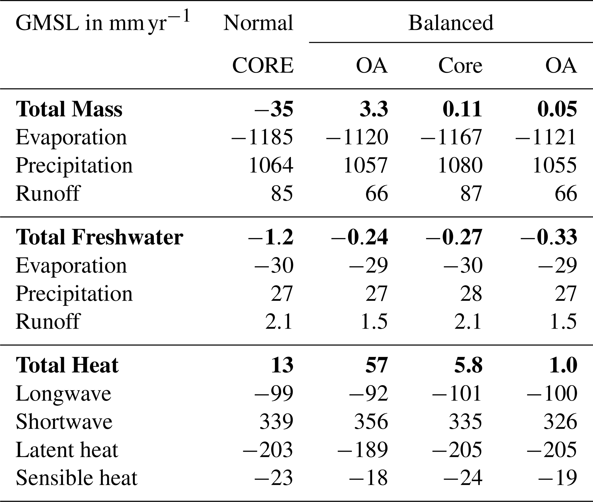
Table 2 Area weighted GMSL rise in mm yr⁻¹, calculated using Eq. (2) for surface mass fluxes (first 4 rows), freshwater fluxes (row 5–8) and heat fluxes (row 10–14). Mass and freshwater fluxes are due to evaporation, precipitation, and runoff, while heat fluxes include radiative fluxes (longwave and shortwave) and turbulent fluxes of latent heat and sensible heat. Bold indicate their sums. See also Sects. 2.2, 4.1-4.3, Eq. (4), 5 and Figs. 1, 2 and 3.

4 Results

This section discusses the results of the quantification of local sea level evolution and GMSL rise due to the different processes described in Sect. 2, in combination with the data described in Sect. 3. The results are presented as spatial maps of sea level rise in mm yr⁻¹, and their global integrals. The given numbers for sea level rise and GMSL rise represent annual mean values, based on a standard year (see Sect. 3).

4.1 GMSL rise due to mass fluxes

Here the direct impact of ocean mass fluxes on sea level rise is discussed (Sect. 2.1, Eq. 4). The indirect impact of mass fluxes on the salinity budget (Eq. 5) are discussed in Sect. 4.2. The largest contributions to GMSL is due to Precipitation P (just over 1100 mm yr⁻¹) and evaporation E (just below $-\mathrm{1100}\mathrm{mm}{\mathrm{yr}}^{-\mathrm{1}}$), and are of opposite sign. Some precipitation falls on land and enters back via river runoff, which is why precipitation is a bit smaller than evaporation and the difference is about the same as that from river runoff and of the order of 65–85 mm yr⁻¹ (Table 2). The different impact on GMSL between CORE and OA due to E, R and P is 65, 19 and 7 mm yr⁻¹, respectively. For R this is probably related to Antarctic runoff added in the CORE product that is not included in OA. For E and P such differences may arise from different bulk transfer algorithms, calibration protocols and reason for which a product is designed. The total difference in GMSL rise between CORE and OA is about 40 mm yr⁻¹, ten times the observed rates of current sea level rise. This means that uncertainties between the products, also swamp the impact of poorly represented barystatic sea level changes of approximately 2 mm yr⁻¹. This clearly indicates the difficulty to accurate represent mass fluxes into the ocean and the impact this could have on sea level rise calculations.

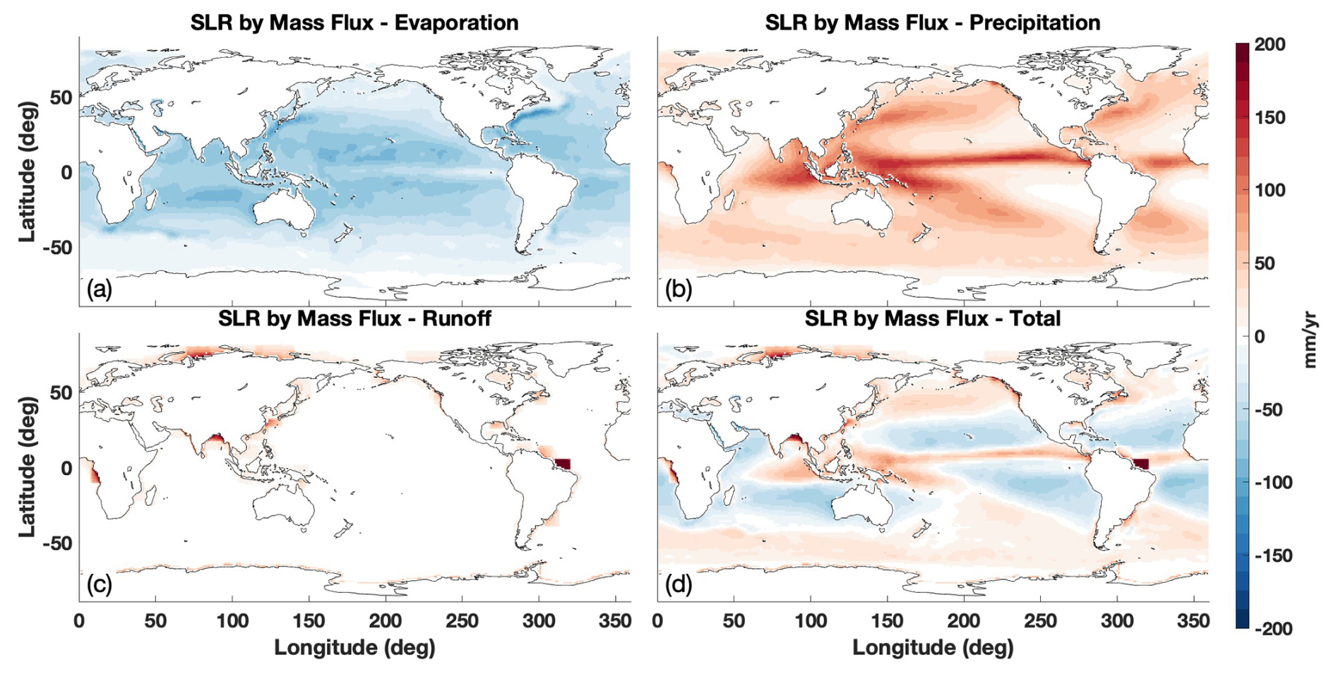
Resulting spatial patterns of sea level evolution due to E, P and R are a direct reflection of well-known evaporation, precipitation and runoff patterns (Fig. 1). Sea level decreases in subtropical regions where evaporation dominates, while sea level increases at higher latitudes and equatorial regions where precipitation dominates (Fig. 1d).

When examining the GMSL changes due to the constructed balanced mass flux products of CORE and OA (Sect. 3.5.1 and Appendix E), the net change in GMSL is of the order of 0.1 mm yr⁻¹, similar to that found by (Griffies and Greatbatch, 2012) in a numerical model. This is a consequence of mass entering the ocean at higher densities (higher latitudes), while leaving the ocean at lower densities (lower latitudes, Eq. 1).

Figure 1 The spatial impact of mass fluxes on sea level rise (mm yr⁻¹) due to Evaporation (a), Precipitation (b), Runoff (c) and their sum (d) for the CORE dataset. Derivations and discussion of these terms are found in Sects. 2.1, 3.5, 4.1, Eq. (4) and Table 2.

4.2 GMSL rise due to the surface freshwater flux

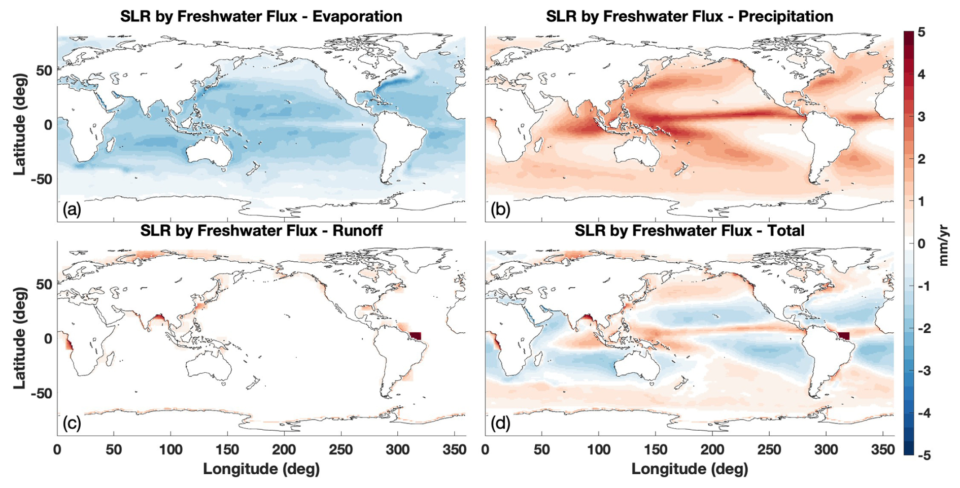
The mass flux (Eq. 3) is also a freshwater flux (Eq. B1) that can be converted into an equivalent salt-flux that alters salinity and thereby density and sea level (Sect. 2.2, Huang, 1993; Nurser and Griffies, 2019; Groeskamp et al., 2019b). The difference between the mass flux and salt flux is only a factor βS_A , meaning that the impact of the salt fluxes on local and GMSL rise is almost 40 times smaller than the direct impact of the individual mass flux terms (Table 2). The impact on GMSL rise due to freshening resulting from precipitation is about 27 mm yr⁻¹, a bit smaller than the impact from evaporation of about $-\mathrm{30}\mathrm{mm}{\mathrm{yr}}^{-\mathrm{1}}$ (Table 2). The residual is covered by the impact on freshening by river runoff (about 2 mm yr⁻¹). Resulting patterns of sea level evolution are different from E, P and R by the factor βS_A , but overall comparable (Fig. 2). Hence, as for the mass flux, sea level decreases in subtropical regions where evaporation dominates, while sea level increases at higher latitudes and equatorial regions where precipitation dominates (Fig. 2d).

The net impact of freshwater fluxes is about $-\mathrm{1}\mathrm{mm}{\mathrm{yr}}^{-\mathrm{1}}$, with the difference between OA and CORE being about the same size and thus of the same order as observed GMSL rise. As for the balanced mass flux products, the resulting “nonlinear haline expansion” leads to a GMSL change of about $-\mathrm{0.3}\mathrm{mm}{\mathrm{yr}}^{-\mathrm{1}}$ for both products, which is of the same order of magnitude as found by Griffies and Greatbatch (2012). This is nonzero as the balanced mass flux is weighted by the factor βS_A, which leads to a net GMSL rise that is non-negligible, but almost an order of magnitude smaller than observed GMSL rise.

Figure 2 The spatial impact of freshwater fluxes on sea level rise (mm yr⁻¹) due to Evaporation (a), Precipitation (b), Runoff (c) and their sum (d). Results are shown for the CORE dataset. Derivations and discussion of these terms are found in Sects. 2.2, 3.5, 4.2, Eq. (5) and Table 2.

4.3 GMSL rise due to the surface heat flux

This section presents the effect of the sensible heat flux, latent heat flux, and long-wave heat flux that are exchanged at the oceans surface on local and GMSL rise (Sect. 2.2). Also, the impact on GMSL rise due to shortwave radiative heat flux is presented, that may penetrate deeper into the ocean (Sect. 3.6, Table 2 and Fig. 3). The shortwave heat flux leads to an increase in sea level, where the other heat fluxes lead to a decrease. Their individual impacts on GMSL vary from $-\mathrm{200}-\mathrm{350}\mathrm{mm}{\mathrm{yr}}^{-\mathrm{1}}$ (Table 2). The total net impact of heat flux is about 10–50 mm yr⁻¹, i.e. with a difference between the two products of about 40 mm yr⁻¹, comparable to that due to global mass fluxes. This difference is not unexpected as heat flux products are notoriously difficult to close (Josey et al., 1999; Yu, 2019). A net global heat flux of 0.3 W m⁻² is enough to explain the observed increase in global heat content (Domingues et al., 2008; Ishii and Kimoto, 2009; Levitus et al., 2012; Lyman and Johnson, 2013), while imbalances up to 30 W m⁻² are not uncommon for available heat flux products (Balmaseda et al., 2015; Valdivieso et al., 2017). The CORE and OA flux products have some of the largest difference in net heat flux (Valdivieso et al., 2017), meaning that these results should be a good indication of the range that can be expected from the impact of heat fluxes on GMSL.

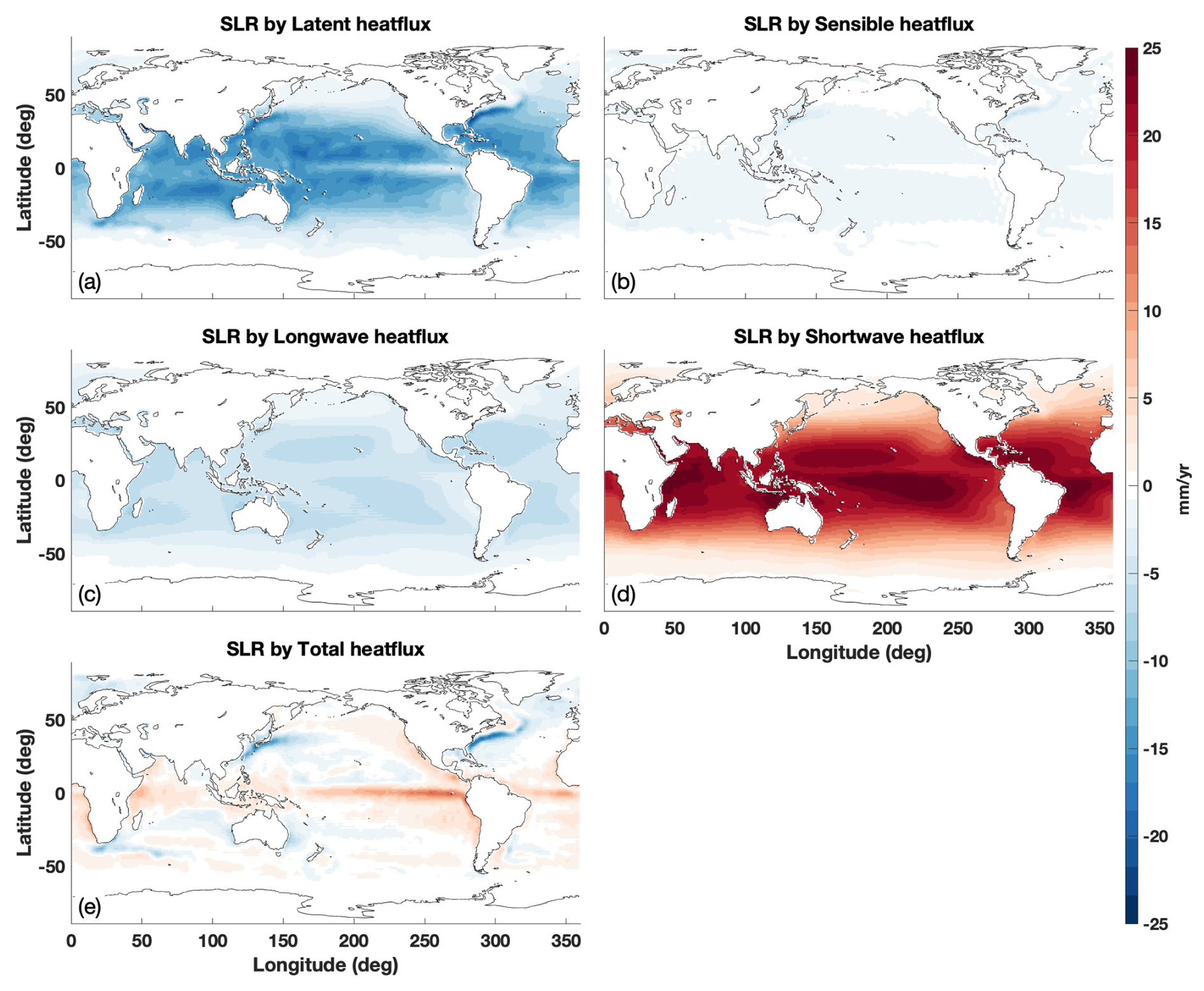
Figure 3 The spatial impact of heat fluxes on sea level rise (mm yr⁻¹) due to latent heat flux (a), sensible heat flux (b), longwave heat flux (c), shortwave heat flux (d) and their sum (e). For SWR penetration the Morel and Antoine (1994) parameterization is used (Eq. B7). Derivations and discussion of these terms are found in Sects. 2.2, 3.5, 4.3, Eq. (5), and Table 2.

Resulting patterns of sea level evolution (Fig. 3) are a direct reflection of heat flux patterns themselves that can be found in many different studies (Josey et al., 1999; Yu, 2019; Tang et al., 2024). Of interest is the distribution of these fluxes, showing warming around the equator and cooling at western boundary currents and higher latitudes (Fig. 3e). As the thermal expansion coefficient can vary up to a factor of 10 (especially with latitude), this leads to differently weighted impact of warming and cooling on sea level.

Nonlinear thermal expansion is calculated using the balanced heat flux products (so no expansion due to net warming, see Sect. 3.5.1) and estimated to be 1–6 mm yr⁻¹. This is comparable to the 10 mm yr⁻¹ found by Griffies and Greatbatch (2012) (their Fig. 7). Hence, both the magnitude of the nonlinear thermal expansion, as well as the difference between the products, is of the same order as the observed GMSL rise (4 mm yr⁻¹). The differences are related to different emphases between products in which heat leaves or enters the ocean, demonstrating the importance of carefully constructing heat flux products. Note that the impacts from both the nonlinear haline contraction and mass fluxes are about an order of magnitude smaller than those from nonlinear thermal expansion (Table 2). In Sect. 4.6 the balance between densification upon mixing and nonlinear thermal and haline expansion is examined.

4.4 GMSL rise due to different SWR penetration parameterizations

The total incoming SWR at the surface is vertically redistributed according to some vertical structure function F(z) (Sect. 2.2, or Eq. B8). This means that a part of the heat reaching the surface is actually accumulating and transforming water below the surface. Most often sub-surface temperatures will be cooler with a smaller thermal expansion coefficient α, and thus a net smaller volume increase compared to the hypothetical situation in which all SWR is absorbed at the surface. The results in row 11 of Table 2 were computed using the vertical distribution function of Morel and Antoine (1994) (Eq. B7). When the other two specified functions (Sect. 4.4) are applied to the balanced products for CORE, the observed change in GMSL due to the total heat flux is 4.7, 5.8, and 6.7 mm yr⁻¹ for F_PS77, F_MA94 (as above) and F_SF, respectively. Taking the balanced products for OA, this gives −0.05, 1.0 and 2.0 mm yr⁻¹ for F_PS77, F_MA94 (as above) and F_SF, respectively. As F_PS77 allows for the deepest penetration, this will lead to the least increase, followed by F_MA94 and F_SF. For the unbalanced heatflux products the difference due to different SWR parameterizations are similar (not shown). In conclusion, GMSL rise can change 1.0 mm yr⁻¹, depending on the choice of SWR depth penetration parameterization.

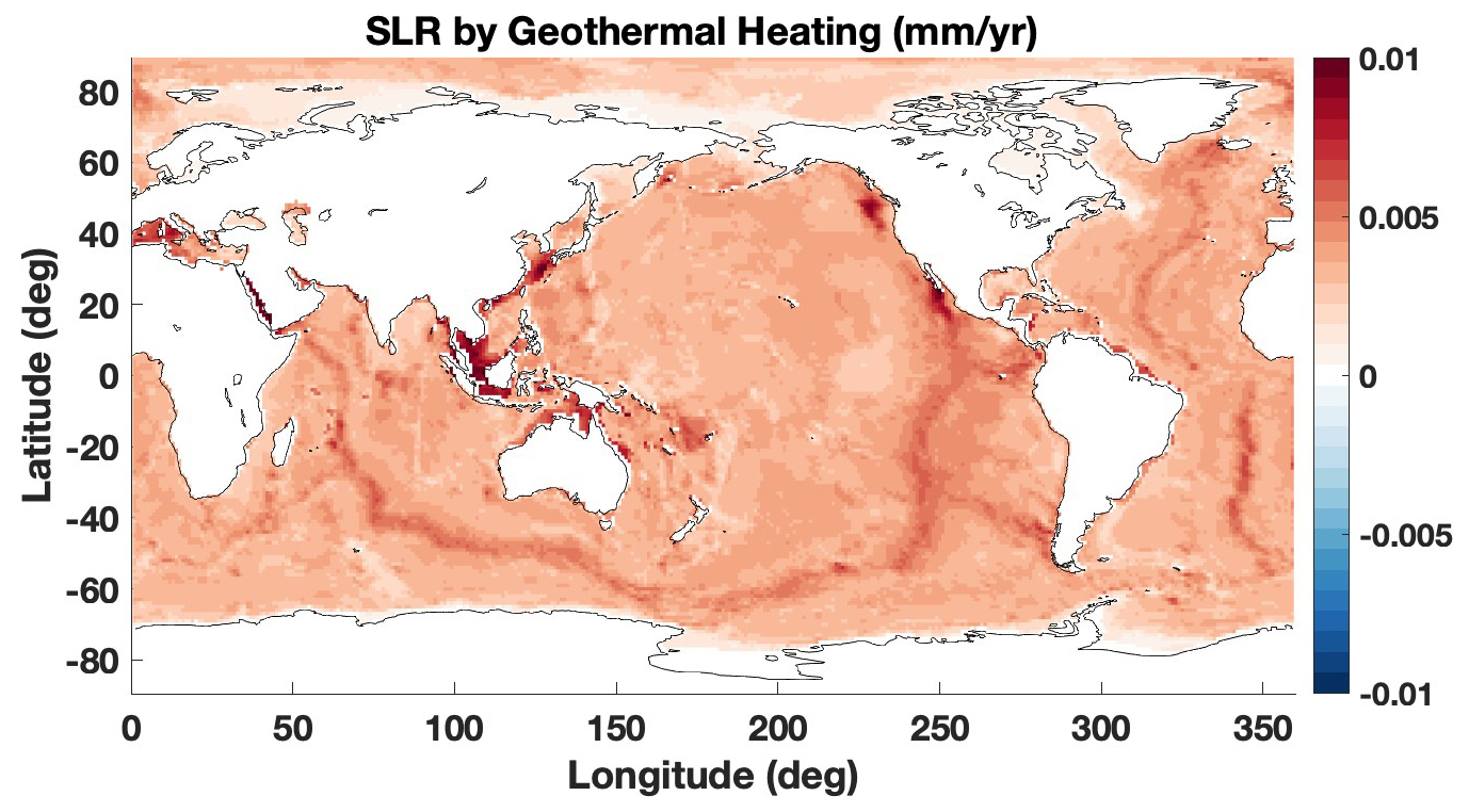
4.5 GMSL rise due to geothermal heating

Geothermal heat injection from the sea floor leads to sea water expansion and local sea level rise. This predominantly occurs along ocean ridges, with additional hot-spots in the Caribbean Sea and the waters around South East Asia (Fig. 4). The large ocean basins have values that are an order of magnitude lower, but cover large surface areas. The total impact of geothermal heating on GMSL is 0.08 mm yr⁻¹. This is relatively small compared to other processes (Table 6) and is exactly similar to that calculated in a numerical model (Griffies and Greatbatch, 2012) (their Table 1).

Figure 4 The spatial impact on sea level rise (mm yr⁻¹) by geothermal heating, which is derived and discussed in Sects. 2.2, 3.5, 4.5, Eq. (5), and Table 6.

4.6 GMSL rise due to mixing

Here the impact on GMSL due to mixing processes is quantified (Sect. 2.3, Eq. 6). The impact on GMSL rise by both constant diffusivities as well as the more realistic spatially varying diffusivities (Sect. 3) are compared and contrasted. This gauges the range of possible outcomes of the impact on GMSL rise due to using different mixing parameterizations. The results for a constant diffusivity are simply proportional to the diffusivity, and can therefore easily be rescaled with a different constant diffusivity in mind.

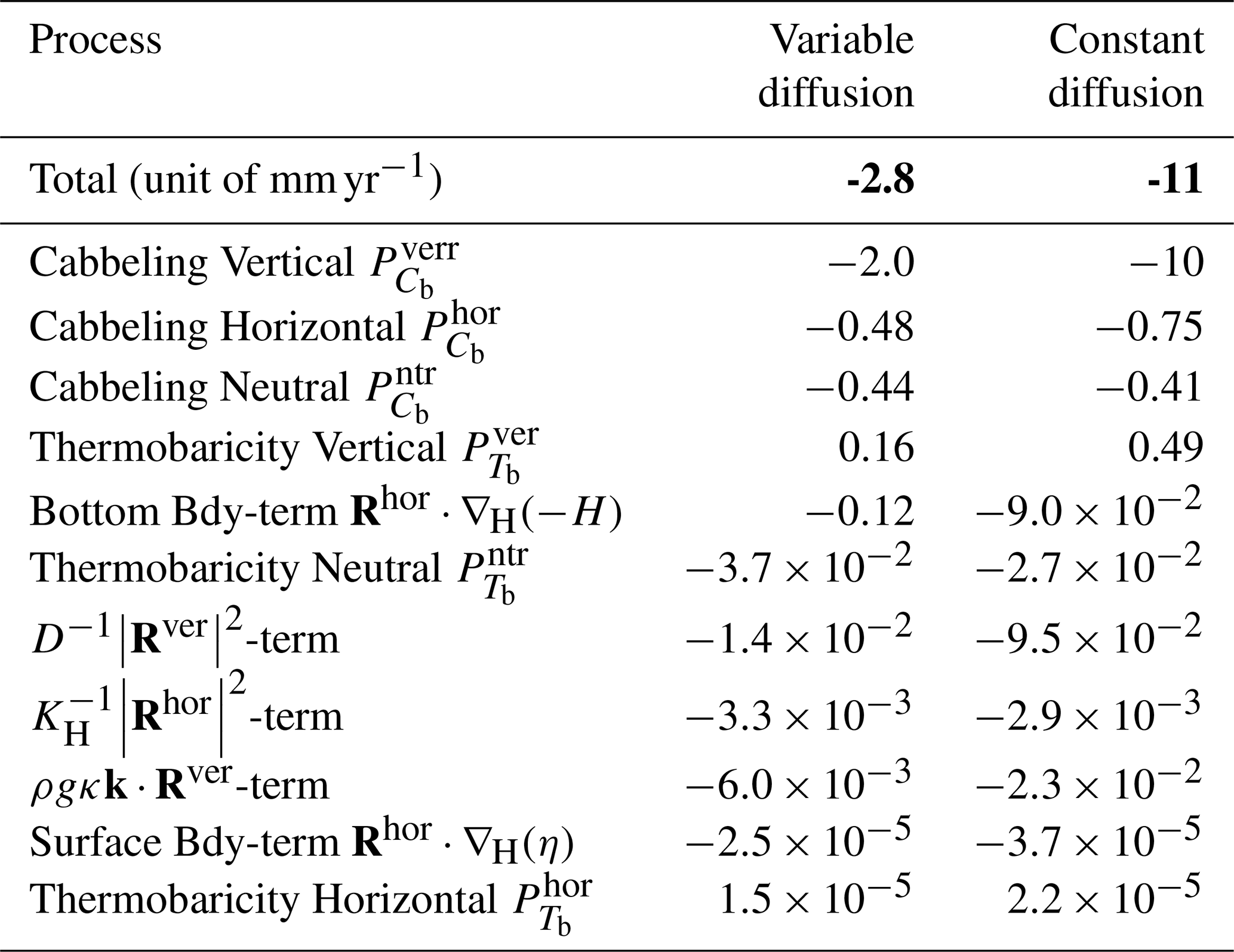
For variable diffusivities, the largest impact on GMSL is by vertical cabbeling ($-\mathrm{2}\mathrm{mm}{\mathrm{yr}}^{-\mathrm{1}}$), and to a lesser extent by horizontal ($-\mathrm{0.4}\mathrm{mm}{\mathrm{yr}}^{-\mathrm{1}}$) and neutral cabbeling ($-\mathrm{0.5}\mathrm{mm}{\mathrm{yr}}^{-\mathrm{1}}$). Together these processes are decreasing GMSL with a rate of about $-\mathrm{3}\mathrm{mm}{\mathrm{yr}}^{-\mathrm{1}}$ (Table 3). Somewhat important are vertical thermobaricity (0.2 mm yr⁻¹) and the bottom boundary condition term ($-\mathrm{0.1}\mathrm{mm}{\mathrm{yr}}^{-\mathrm{1}}$). All other mixing-related terms have an almost negligible impact on GMSL rise (Table 3).

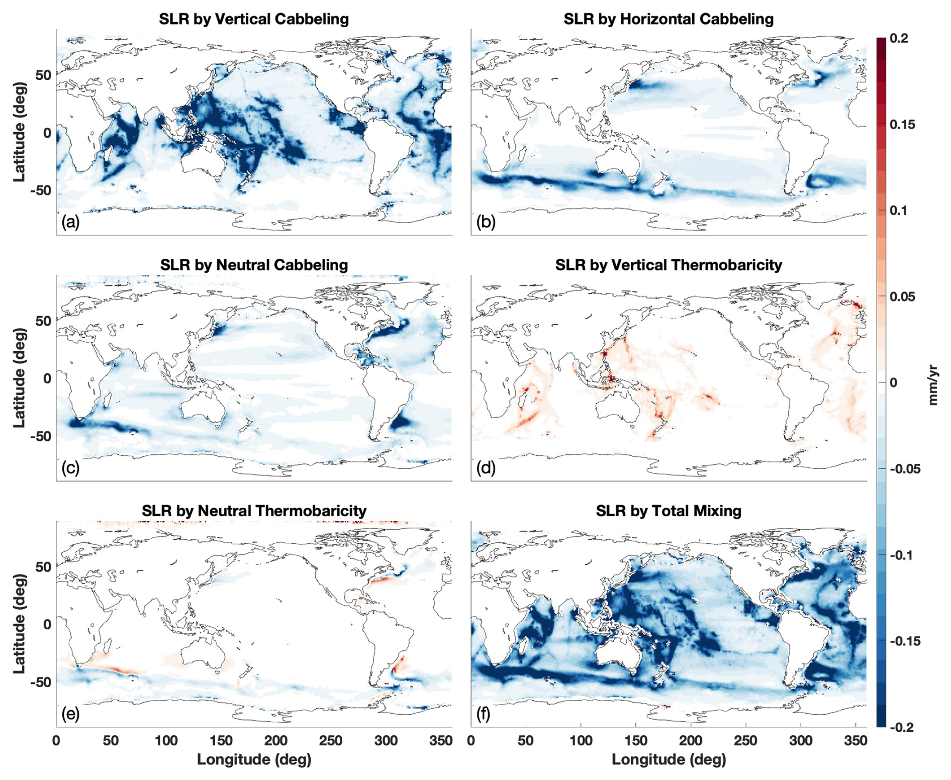
Figure 5 The spatial impact on sea level rise (mm yr⁻¹) by the most important mixing terms, due to vertical cabbeling (a), horizontal cabbeling (b), neutral cabbeling (c), vertical thermobaricity (d), Neutral Thermobaricity (e) and the sum of all mixing terms (f), including the ones shown in Fig. 6. The mixing terms are derived and discussed in Sects. 2.3, 3.2, 4.6, Eq. (6), and Table 3.

Table 3 Area weighted GMSL rise in mm yr⁻¹, calculated using Eq. (2) for different mixing terms as described in Sect. 2.3 and Eq. (6) and shown in Figs. 5 and 6.

The use of a constant diffusivity is an overly simplistic alternative that instead might overestimate the impact of vertical mixing and results in $D_{\text{constant}}>D(x,y,z)$ in the upper 2500 m of the ocean. This explains the difference of a factor 5 in GMSL rise due to vertical cabbeling, between using a variable or constant vertical diffusivity D. The best way to narrow down this estimate is to first include an observational-based estimate of a surface layer boundary mixing scheme, which is beyond the scope of this study.

Taken together, the total impact of all mixing on GMSL rise is between −3 and $-\mathrm{11}\mathrm{mm}{\mathrm{yr}}^{-\mathrm{1}}$. This indicates that both the impact of mixing itself, as well as the difference between mixing parameterizations, are of the same order as the observed GMSL rise. In addition, the impact of mixing is comparable in magnitude and of opposite sign to the impact from nonlinear thermal expansion (Table 2, Sect. 4.3), suggesting that densification upon mixing can counteract expansion due to nonlinear thermal expansion.

Vertical cabbeling takes place where there is vertical mixing by internal waves (de Lavergne et al., 2020) in combination with vertical gradients of temperature and salinity (Eq. C22), which is mostly around topography (Fig. 5a). Although the integrated impact of vertical diffusion on GMSL rise is comparable to that found in Griffies and Greatbatch (2012), the spatial structure of this effect is very different (their Fig. 10a). The differences between these studies is best explained by the different diffusivity parameterizations. Vertical thermobaricity is of opposite sign to cabbeling and smaller, this increasing sea level at locations where vertical cabbeling is also strong (Fig. 5d).

Neutral temperature and salinity gradients are particularly strong in the Southern Ocean at mid-depths, near western boundary currents and to a lesser extent in the major ocean basins (Groeskamp et al., 2019a). The mesoscale diffusivity are particularly strong near western boundary currents and in some of the subtropical regions (Groeskamp et al., 2020). Together this means the impact of neutral cabbeling on sea level rise is mostly centered around western boundary currents and to some extent in the Southern Ocean (Fig. 5c). This is expected, as other studies also found these location to be a hotspot for neutral cabbeling (Groeskamp et al., 2016; Klocker and McDougall, 2010; Griffies and Greatbatch, 2012; Urakawa and Hasumi, 2012). For similar reasons, neutral thermobaricity is large in many of the same places as neutral cabbeling, but is generally smaller and can lead to both sea level rise and fall (Fig. 5e). Horizontal cabbeling is defined using the same diffusivity as neutral mixing, but only in the mixed layer. This means it is more pronounced where mixed layers are also deeper (Fig. 5b), such as in the Southern Ocean and the North Atlantic (de Boyer Montégut et al., 2004).

Overall mixing decreases sea level (Fig. 5f), with the largest impact where the different cabbeling processes are strong. The spatial distribution of the small (negligible) terms are shown for completeness (Fig. 6), but not further discussed.

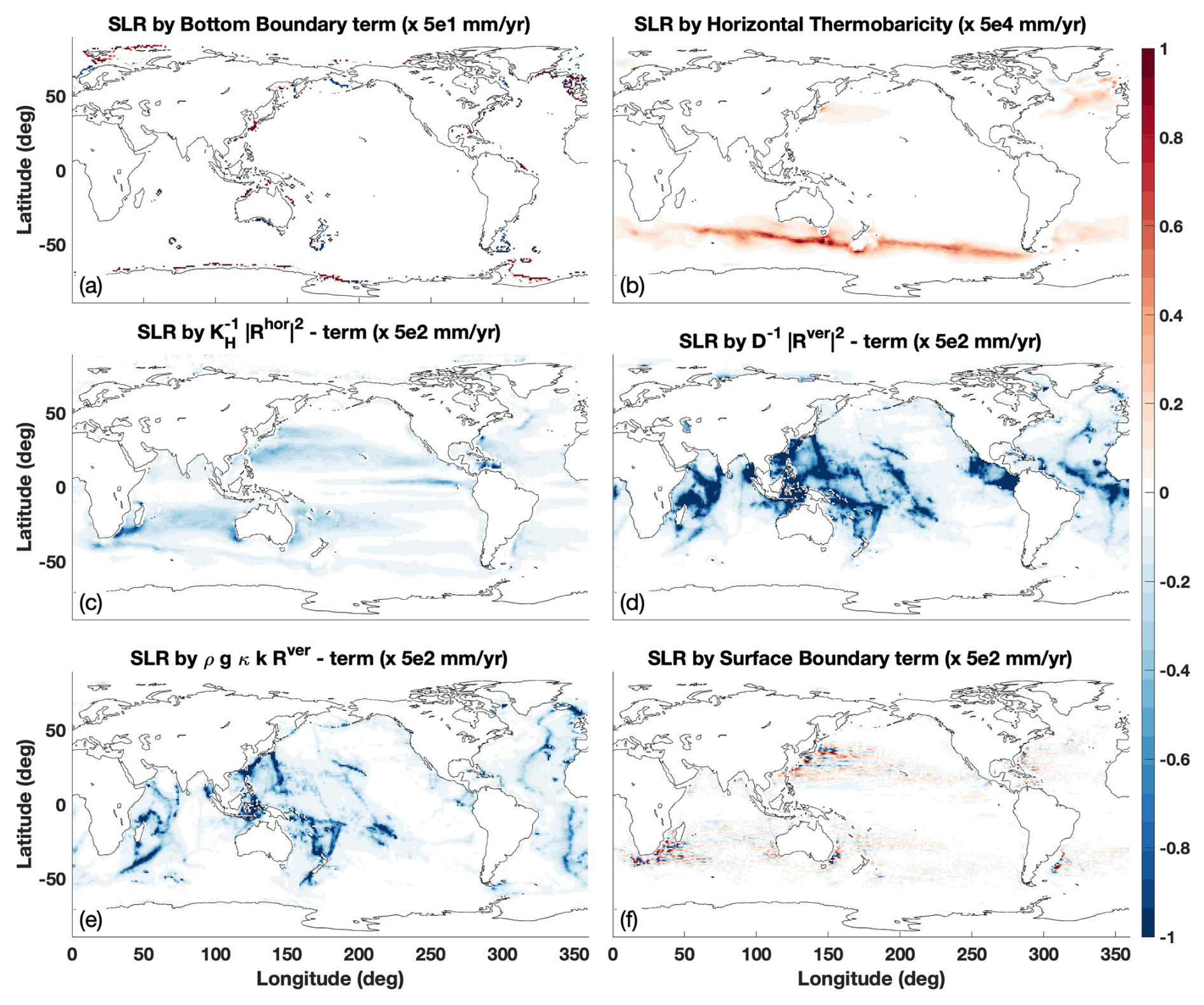
Figure 6 The spatial impact on sea level rise (mm yr⁻¹) by the mixing terms with a small impact. Shown are the bottom boundary term (a), horizontal thermobaricity (b), diffusion-density interaction with horizontal mixing $K_{\mathrm{H}}^{-\mathrm{1}}|{\mathbf{R}}^{\text{hor}}{|}^{\mathrm{2}}$-term (c), the diffusion-density interaction with vertical mixing $D^{-\mathrm{1}}|{\mathbf{R}}^{\text{ver}}{|}^{\mathrm{2}}$-term (d), diffusion-density interaction with horizontal mixing ρgκk⋅R^ver-term (e), and the surface Boundary term R^hor⋅∇_H(η) (f). Note the multiplication factor given in the title, which is used for all terms to have the same color-scale. The mixing terms are derived and discussed in Sects. 2.3, 3.2, 4.6, Eq. (6), and Table 3.

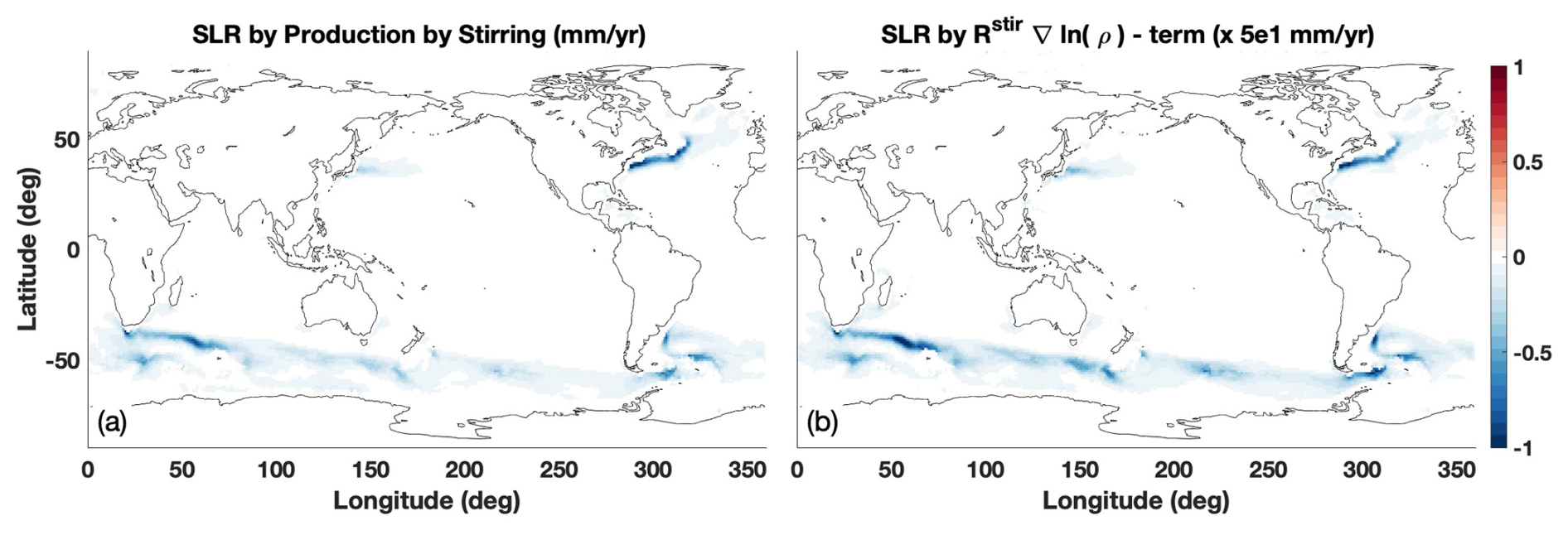
4.7 GMSL rise due to stirring

The impact of stirring on sea level (Sect. 2.4, Eq. 11) is investigated by comparing results using a constant mesoscale diffusivity to those using a spatially varying mesoscale diffusivity (Sect. 3.2). There are only three terms contributing to stirring, of which the first term is zero after global integration (Eq. 11). Of the remaining two terms, the production term P_stir has a non negligible impact on GMSL rise of about −0.4 to $-\mathrm{0.6}\mathrm{mm}{\mathrm{yr}}^{-\mathrm{1}}$ (Table 4), that is about 8 times smaller than observed GMSL rise.

Table 4 Area weighted GMSL rise in mm yr⁻¹, calculated using Eq. (2) for stirring. See also Sects. 2.4, 4.7, Eq. (11) and Fig. 7.

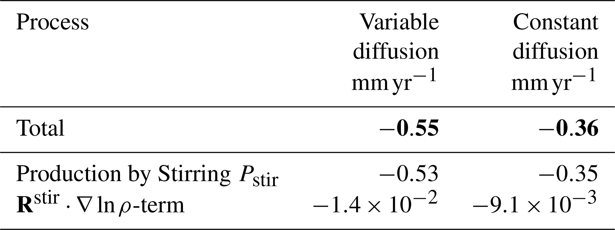
The stirring parameterization includes a factor K S (Eq. D6), causing the main impact on sea level to be where the combination of both neutral slopes and mesoscale diffusivity are large. This is between 40 an 50° S and in western boundary currents (Fig. 7). Although its global mean impact is moderate, it could locally be important.

Figure 7 The spatial impact of the stirring terms on sea level rise (mm yr⁻¹), due to stirring production term (a) and the R^stir⋅∇ln ρ-term (b). Note the multiplication factor given in the title of panel b. The stirring terms are derived and discussed in Sects. 2.4, 3.2, 4.7, Eq. (11), and Table 4.

4.8 GMSL rise due to Non-Neutrality

Here the impact of non-neutrality on GMSL is quantified (Sect. 2.5, Eq. 14). As explained in Sect. 3.3, two methods are used for calculating neutral slopes and gradients. The results from the VENM algorithm is used as perfectly neutral in Eq. (14), while using the results from the local method as ntr. As VENM is not perfectly neutral, the results should be interpret as the order of magnitude of the improvement that can be made when accurate neutral physics is implemented.

The first (non-divergent) term in Eq. (14) has no net contribution to GMSL rise by construction and is discussed in Sect. 4.9. The three non-neutral terms that are related to R^ntr (Eq. 14), all have very small contribution to GMSL (Table 5, Fig. 8c–e). Note these can be directly calculated using the gradients obtained from the VENM method, and these terms would be larger when using the local method as that is much less neutral and more irregular (Groeskamp et al., 2019a). However, these terms are small, even when using the local method, and are not further discussed.

Table 5 Area weighted GMSL rise in mm yr⁻¹, calculated using Eq. (2) for non-neutral terms. See also Sects. 2.5, 4.8, Eq. (14) and Fig. 8.

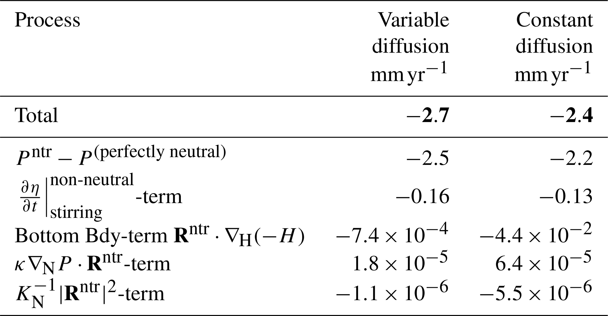
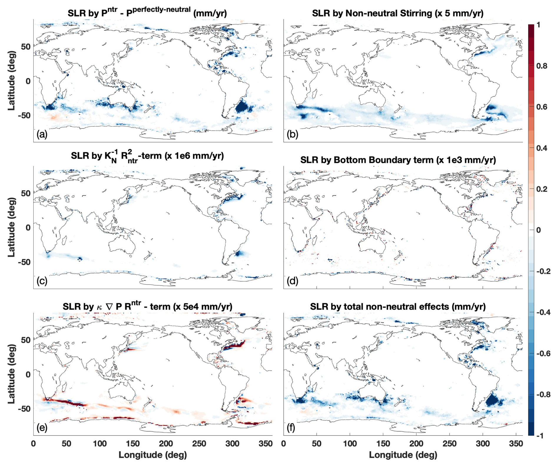
Figure 8 The spatial impact of the non-neutral terms on sea level rise (mm yr⁻¹), due to the production terms (a), the stirring production term (b), the $K_{\mathrm{N}}^{-\mathrm{1}}|{\mathbf{R}}^{\text{ntr}}{|}^{\mathrm{2}}$-term (c), the bottom boundary term (d), the κ∇_NP⋅R^ntr-term (e), and the sum of all these terms (f). Note the multiplication factor given in some of the titles, which is used for all terms to have the same color-scale. The non-neutral terms are derived and discussed in Sects. 2.5, 3.3, 4.8, Eq. (14), and Table 5.

The main impact of non-neutrality to GMSL rise comes from the neutral cabbeling and thermobaricity terms ($-\mathrm{2.5}\mathrm{mm}{\mathrm{yr}}^{-\mathrm{1}}$), and to a lesser extent from eddy stirring ($-\mathrm{0.2}\mathrm{mm}{\mathrm{yr}}^{-\mathrm{1}}$). The impact of calculating these terms using different methods is in total about -3 mm yr⁻¹, with a small impact from the difference in diffusivity. This means that the use of the local method makes an error of at least the same order of magnitude as observed GMSL rise rates themselves.

4.9 GMSL redistribution terms

The four redistribution terms that have local impact on sea level, but no net impact on GMSL, are from ocean currents (Eq. 10 and Sect. 2.4), from horizontal diffusion (Eq. 6 and Sect. 2.3), from neutral diffusion (a non-neutrality term, Eq. 14 and Sect. 2.5) and from stirring (Eq. 11 and Sect. 2.4). The redistribution terms have a large impact on local sea level rise (except the neutral term). The largest impact on local sea level is by dynamical sea level changes (Fig. 9d). In all cases, clear patterns of positive and negative change exist due to the divergence operator (Fig. 9). The shape and location of these patterns are related to specific processes. For example; the horizontal diffusion redistributes volume from the subtropics to the equator, while stirring does this within western boundary currents. Overall these results are not further examined, but the figures are provided for completeness.

Figure 9 The spatial impact of the redistribution terms on sea level rise (mm yr⁻¹), due to horizontal mixing divergence (a), non-neutral divergence (b), stirring divergence (c) and ocean dynamics (d). Note the multiplication factor given in the titles, which is used for all terms to have the same color-scale. The divergence terms are discussed in Sect. 4.9.

5 Summary and discussion

Observation-based mass and heat fluxes are by far the largest contributors to GMSL changes, but they are notoriously hard to balance due to a lack of observational constraints. For example, the GMSL rise estimates based on the mass flux ($-\mathrm{35}-\mathrm{3}\mathrm{mm}{\mathrm{yr}}^{-\mathrm{1}}$, Table 6) or the heat flux (13–57 mm yr⁻¹, Table 6) are both about ten times larger than the observed GMSL rise (4 mm yr⁻¹). For comparison, Griffies and Greatbatch (2012) found the net impact of the ocean mass flux on sea level to be 0.8 mm yr⁻¹ in a numerical model environment (their Fig. 2). The impact on GMSL rise estimated from different heat and mass fluxes is also about ten times larger than the observed GMSL rise. The main source of these differences for mass flux products is the representation of ocean evaporation and precipitation processes (Sect. 4.1 and Table 6), which overwhelm uncertainties in the representation of barystatic sea level rise. Similarly, different bulk formulas and choices in calculating heat fluxes may have a large impact on GMSL rise. Improving the mass and heat flux products is beyond the scope of this study. This study only gauges the magnitude of their impact and uncertainties. With such large inaccuracies in estimating GMSL rise, it is not yet possible to close the GMSL budget using the sum of the contributing processes, i.e., the bottom-up approach.

Table 6 Summary of the area weighted GMSL rise in mm yr⁻¹ for the different processes discussed in this paper. The results from the balances mass and heat flux product are given in brackets.

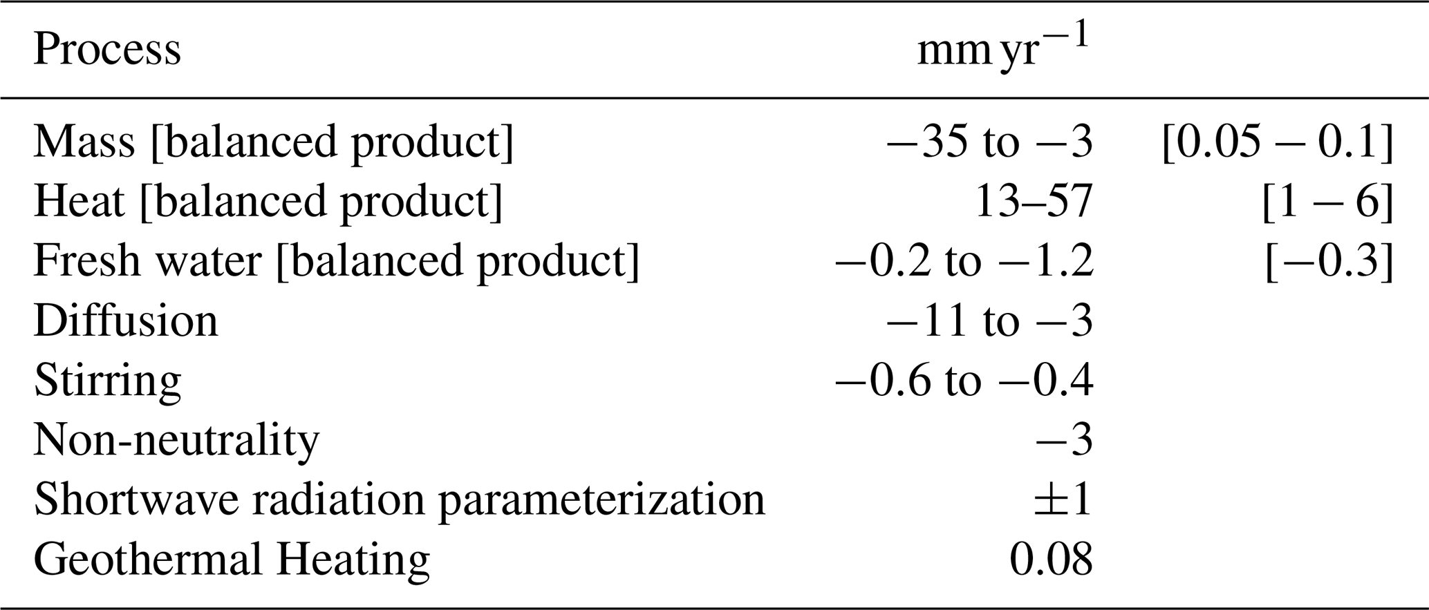
Therefore, this study also uses heat and mass flux products that are artificially forced to have a globally integrated net-zero mass and heat flux (Appendix E). This approach is somewhat comparable to numerical ocean models that remove global mass imbalances at each time step to prevent long-term drift (Griffies, 2012). For the balanced mass fluxes, the impact on GMSL is about 0.1 mm yr⁻¹. The residual is a consequence of nonlinear weighting of the mass fluxes by the ocean surface density (Eq. 4). The mass flux can also be recalculated into an equivalent salt flux (using the factor βS_A, Eq. B8), which affects density and changes GMSL by about $-\mathrm{0.3}\mathrm{mm}{\mathrm{yr}}^{-\mathrm{1}}$.

The impact of balanced heat flux products on GMSL is reduced by an order of magnitude compared to the unbalanced products to 1–6 mm yr⁻¹. This is not due to “regular” thermal expansion from climate change warming, as there is net-zero heat going into the ocean. Instead this is due to nonlinear thermal expansion as a consequence of the heat fluxes being weighted by the thermal expansion coefficient that varies strongly with temperature, before global integration (Eq. B8). Note that (slight) differences in spatial variation between the two heat flux products, lead to a difference in GMSL rise estimate of 5 mm yr⁻¹. Hence, both the value and the uncertainty in calculating the nonlinear thermal expansion are of similar magnitude as the observed GMSL rise of 4 mm yr⁻¹.

The combination of horizontal, neutral, and vertical mixing leads to densification upon mixing and subsequent reduction in GMSL of −3 to $-\mathrm{11}\mathrm{mm}{\mathrm{yr}}^{-\mathrm{1}}$. This is mostly due to vertical mixing, and to a lesser extent due to horizontal and neutral mixing. Griffies and Greatbatch (2012) found that the KPP-mixing scheme for the surface boundary layer (Large et al., 1994; Van Roekel et al., 2018) has a comparable impact on GMSL rise as vertical mixing over the entire ocean. The small-scale diffusivities used in this study (de Lavergne et al., 2019) to estimate the impact of vertical mixing on GMSL rise do not include surface boundary layer parameterizations and therefore underestimate surface boundary layer mixing processes. The impact of vertical mixing could therefore be underestimated by about a factor of 2. Note that thermobaricity, a nonlinear effect related to pressure and temperature changes, can lead to both a sea level rise and fall. However, this term is in general an order of magnitude smaller than the impact of densification upon mixing. The range of the impact of mixing on GMSL rise depends mostly on the parameterizations used for mixing diffusivity (mixing strength).

It is concluded here that (1) mixing itself has a first-order effect on GMSL rise, and (2) differences between mixing strength parameterizations have an impact on GMSL of the same order as the observed GMSL rise. This means that mixing matters for GMSL. This is of interest for numerical modeling purposes because mixing parameterizations can vary strongly between models (Pradal and Gnanadesikan, 2014), thereby differently impacting GMSL rise budgets. Stirring of heat and salt by mesoscale eddies decreases GMSL rise at a rate of −0.4 to $-\mathrm{0.6}\mathrm{mm}{\mathrm{yr}}^{-\mathrm{1}}$, which is important but smaller than the impact of diffusion.

In this study, both nonlinear thermal expansion and densification upon mixing are separately quantified and are, within the range of the estimates, indeed of the same order of magnitude but of opposite sign. Note that if the ocean were of uniform temperature and salinity, both effects would not exist. Hence, these two processes will always occur together: as heat fluxes create extremes and induce nonlinear thermal expansion, mixing acts to homogenize the ocean, causing densification upon mixing. As models include choices about mixing parameterizations and boundary flux products, this leads to some balance between nonlinear thermal expansion and densification upon mixing. It is complex to understand what impact these choices have on the GMSL budgets and related predictions of future sea level rise. In addition, the time scales related to the impact of densification upon mixing and nonlinear thermal expansion are likely very different, implying a time lag between the effects of these two processes. Understanding this interplay is of interest but beyond the scope of this study. This study thus emphasizes the importance of ocean mixing, not only for circulation (de Lavergne et al., 2022; Holmes et al., 2022), climate (Melet et al., 2022) and biogeochemical processes (Lévy et al., 2022; Spingys et al., 2021), but also for sea level rise (Gille, 2004; Jayne et al., 2004).

This study shows that the way neutral physics is implemented, has a first order effect on GMSL rise. Incorrect implementation of neutral physics leads to additional mixing and related densification upon mixing. Differences in neutral physics methods used to calculate neutral slopes and gradients lead to a GMSL difference of about $-\mathrm{3}\mathrm{mm}{\mathrm{yr}}^{-\mathrm{1}}$, which is a leading-order term. This results in a low bias, something also hinted at by Gille (2004) in a numerical model. This emphasizes the need to integrate the most advanced and accurate methods for neutral physics calculation in numerical models for predicting future sea level rise (Groeskamp et al., 2019a; Shao et al., 2020).

Different ways of parameterizing the vertical distribution of shortwave radiation cause differences in which water layers are heated. Parameterizations that allow for deeper penetration heat colder waters. As colder water has a lower thermal expansion coefficient, heating cold water leads to less sea level rise than heating warm water. Parameterizations that allow deeper penetration of shortwave radiation will thus have a smaller impact on GMSL rise. Differences in sea level rise between such parameterizations lead to GMSL rise differences of about $\pm \mathrm{1}\mathrm{mm}{\mathrm{yr}}^{-\mathrm{1}}$. Not only is this a large term, but the effect is unidirectional over time and has the potential to accumulate to 10 cm per century.

6 Conclusions

The sum of barystatic and steric sea level change can explain the observed GMSL rise as derived from tide gauges and satellite altimetry (Moore et al., 2011; Horwath et al., 2022; Frederikse et al., 2020; Church et al., 2011; Ludwigsen et al., 2024; Frederikse et al., 2020). The calculations and methods involved in obtaining the steric and barystatic estimates are derived from large top-down integrals of ocean hydrographies and satellite observations. However, this top-down approach glosses over the impact on the GMSL budget of individual physical oceanographic processes. This study therefore applied a bottom-up approach in which the contributions of individual physical processes to GMSL rise are estimated from observation-based products.

Such processes include, but are not limited to, the impacts of diffusion, stirring, neutral physics, shortwave radiation, and boundary fluxes, all of which alter oceanic density and thus affect GMSL. It is valuable to be able to close the GMSL rise budget, as estimated from observations, by summing the contributions from the physical processes underlying changes in the GMSL rise budget. This provides insight into the fundamental processes behind the observed global sea level rise and how these processes may change in a transient ocean and climate.

This study provides a comparison of both the magnitude and uncertainty of the impact on GMSL by single processes or parameterizations. With the observed GMSL rise currently being about 4 mm yr⁻¹, this indicates that processes causing changes of the order of 1 mm yr⁻¹ can be considered leading order terms in calculating GMSL rise. For accurately closing the GMSL rise budget, one should arguably have an accuracy of about 0.1 mm yr⁻¹. This immediately clarifies that it is not yet possible to close the GMSL budget using the bottom-up approach applied in this study.

For example, this study finds differences in GMSL rise estimates of about 30 and 40 mm yr⁻¹ between different boundary heat flux products or different mass flux products, respectively (Table 6). These estimates would improve if better observation-based constraints were available. Improving the mass and heatflux products is beyond the scope of this study. Instead, this study also used artificially balanced (i.e., globally net-zero) boundary mass and heat flux products for calculating the impacts on GMSL rise. Taken together, this study concludes that:

• It is currently not possible to close the GMSL rise budget using available ocean heat or mass flux products (Sects. 4.1 and 4.3).

• Between different balanced heat flux products (no net global heating), differences in GMSL rise estimates are of the same order as the observed GMSL rise. This indicates that the spatial distribution of a heat flux product plays an important role for the GMSL rise budget (Sects. 4.1 and 4.3).

• Mixing strength parameterizations have a leading-order impact on GMSL rise estimates (Sect. 4.6).

• Implementation of neutral physics has a leading-order impact on GMSL rise estimates (Sect. 4.8).

• The choice of shortwave radiation parameterizations has a leading-order impact on GMSL rise budgets, and its impact accumulates over time (Sect. 4.4).

• Parameterized eddy advection and freshwater fluxes have a second order impact on GMSL (Sects. 4.7 and 4.2).

• Nonlinear thermal expansion and densification upon mixing occur together, are of the same order of magnitude but of opposite sign, and therefore compensate each other. However, different time scales are involved for both processes due to differing physical mechanisms and geographical locations (Sect. 5).

The accuracy of the estimates is limited by both a lack of knowledge and observation-based constraints for several of the physical processes involved (e.g. boundary heat and mass fluxes, mixing, shortwave radiation), as well as due to the complexity to numerically implementing neutral physics. The above points should also be of interest to ocean modelers, as they must make specific choices about how to represent heat fluxes, mixing diffusivities, shortwave penetration, eddy stirring, and neutral physics. All these factors have a non-negligable impact on GMSL rise calculations. It remains unclear how the combination of these choices would impact GMSL rise predictions in, for example, IPCC-class models, as these require significant spin-up and equilibrium time during which some of these errors might balance out–or may lead to the right estimate for the wrong reason. It also raises the question if non-Boussinesq ocean models can accurately capture these impacts or will encounter too large uncertainties to obtain a realistic sea level budget from steric changes. Therefore, these results advocate for a thorough analysis of these processes in both models and observations, to improve understanding of such choices on GMSL rise predictions and increase the accuracy of predicted future sea level rise upon which policy will be based.

Appendix A: The material derivative of density

In Eq. (1), the material derivative of density is given by:

$$\begin{array}{}\text{(A1)}& {\displaystyle \frac{\mathrm{d}\mathit{\rho }}{\mathrm{d}t}}=-\mathit{\alpha }\mathit{\rho }{\displaystyle \frac{\mathrm{d}\mathrm{\Theta }}{\mathrm{d}t}}+\mathit{\beta }\mathit{\rho }{\displaystyle \frac{\mathrm{d}{S}_{\mathrm{A}}}{\mathrm{d}t}}+\mathit{\kappa }\mathit{\rho }{\displaystyle \frac{\mathrm{d}P}{\mathrm{d}t}}.\end{array}$$

Here $\mathrm{d}\mathrm{\Theta }/\mathrm{d}t$, $\mathrm{d}{S}_{\mathrm{A}}/\mathrm{d}t$ and $\mathrm{d}P/\mathrm{d}t$ are the material derivatives of Conservative Temperature Θ, Absolute Salinity S_A and pressure P, respectively. The thermal expansion coefficient α, the saline contraction coefficient β, and the isentropic compressibility κ are given by:

$$\begin{array}{}\text{(A2)}& \begin{array}{rl}{\displaystyle }& {\displaystyle }\mathit{\alpha }=-{\displaystyle \frac{\mathrm{1}}{\mathit{\rho }}}{\displaystyle \frac{\partial \mathit{\rho }}{\partial \mathrm{\Theta }}}{|}_{S_{\mathrm{A}},P},\mathit{\beta }={\displaystyle \frac{\mathrm{1}}{\mathit{\rho }}}{\displaystyle \frac{\partial \mathit{\rho }}{\partial S_{\mathrm{A}}}}{|}_{\mathrm{\Theta },P},\\ {\displaystyle }& {\displaystyle }\mathit{\kappa }={\displaystyle \frac{\mathrm{1}}{\mathit{\rho }}}{\displaystyle \frac{\partial \mathit{\rho }}{\partial P}}{|}_{S_{\mathrm{A}},\mathrm{\Theta }}.\end{array}\end{array}$$

Here the ${|}_{S_{\mathrm{A}},P}$ indicates that the derivative is obtained at constant S_A and P, etc. Changes in density are related to changes in S_A, Θ and P through α, β and κ. Because α, β and κ also depend on S_A, Θ and P, the equation of state is nonlinear. The convergence of heat and salt that can be written as:

$$\begin{array}{}\text{(A3)}& {\displaystyle }& {\displaystyle }\mathit{\rho }{\displaystyle \frac{\mathrm{d}\mathrm{\Theta }}{\mathrm{d}t}}=-\mathrm{\nabla }\cdot \left({\mathbf{J}}_{\text{diff}}^{\mathrm{\Theta }}+{\mathbf{J}}_{\text{stir}}^{\mathrm{\Theta }}\right)+F_{\text{mass}}^{\mathrm{\Theta }}+\mathit{\rho }{F}_{\text{source}}^{\mathrm{\Theta }},\text{(A4)}& {\displaystyle }& {\displaystyle }\mathit{\rho }{\displaystyle \frac{\mathrm{d}{S}_{\mathrm{A}}}{\mathrm{d}t}}=-\mathrm{\nabla }\cdot \left({\mathbf{J}}_{\text{diff}}^{S_{\mathrm{A}}}+{\mathbf{J}}_{\text{stir}}^{S_{\mathrm{A}}}\right)+F_{\text{mass}}^{S_{\mathrm{A}}}+\mathit{\rho }{F}_{\text{source}}^{S_{\mathrm{A}}}.\end{array}$$

Here salt and heat changes due to convergence of diffusive fluxes are given by ${\mathbf{J}}_{\text{diff}}^{\mathrm{\Theta }}$ and ${\mathbf{J}}_{\text{diff}}^{S_{\mathrm{A}}}$ (in tracer $\mathrm{kg}{\mathrm{m}}^{-\mathrm{2}}{\mathrm{s}}^{-\mathrm{1}}$), and include a diversity of mixing processes that are detailed in Sect. 2.3. The minus sign assures positive numbers when heat or salt accumulate (converge). Salt and heat convergence due to advective subgridscale processes or “skew fluxes” are given by ${\mathbf{J}}_{\text{stir}}^{\mathrm{\Theta }}$ and ${\mathbf{J}}_{\text{stir}}^{S_{\mathrm{A}}}$ (in tracer $\mathrm{kg}{\mathrm{m}}^{-\mathrm{2}}{\mathrm{s}}^{-\mathrm{1}}$) (Gent and McWilliams, 1990; Gent et al., 1995; Griffies, 1998; McDougall and McIntosh, 2001). The changes of heat and salt due to boundary mass fluxes are given by $F_{\text{mass}}^{\mathrm{\Theta }}$ and $F_{\text{mass}}^{S_{\mathrm{A}}}$. Meanwhile the source terms $F_{\text{source}}^{S_{\mathrm{A}}}$ and $F_{\text{source}}^{\mathrm{\Theta }}$ (tracer $\mathrm{kg}{\mathrm{m}}^{-\mathrm{3}}{\mathrm{s}}^{-\mathrm{1}}$) contain all other possible direct sources and sinks of salt and heat. Also the impact of pressure variations on density ($\mathit{\kappa }\frac{DP}{Dt}$, the last term in Eq. A1) is not accounted for. This is rationalized because (1) the impact is measurable but small (Dewar et al., 1998) , and (2) Griffies and Greatbatch (2012) showed the impact on GMSL rise of this term is about 1000–10 000 times smaller than recent sea level rise estimates. As this term is difficult to calculate from observation-based products and almost negligible, it is not further investigated in this study.

Appendix B: Specifying the impact of boundary fluxes of salinity and temperature on density and sea level

In this section the impact of mass and source fluxes of salinity and temperature are combined, to express their impact on density and sea level. Surface mass fluxes Q_mass change salinity and temperature through $F_{\text{mass}}^{S_{\mathrm{A}}}$ and $F_{\text{mass}}^{\mathrm{\Theta }}$ in Eq. (A4). Combined, they alter density as follows:

$$\begin{array}{}\text{(B1)}& \begin{array}{rl}{\displaystyle }{F}_{\text{mass}}^{\mathit{\rho }}& {\displaystyle }=\underset{F_{\text{mass}}^{\mathrm{\Theta }}}{\underbrace{-\mathit{\alpha }{Q}_{\text{mass}}({\mathrm{\Theta }}_{\mathrm{m}}-\mathrm{\Theta })\mathit{\delta }(z-\mathit{\eta })}}\\ {\displaystyle }& {\displaystyle }+\underset{F_{\text{mass}}^{S_{\mathrm{A}}}}{\underbrace{\mathit{\beta }{Q}_{\text{mass}}(S_{\mathrm{m}}-S_{\mathrm{A}})\mathit{\delta }(z-\mathit{\eta })}}.\end{array}\end{array}$$

Here $F_{\text{mass}}^{\mathit{\rho }}$ ($\mathrm{kg}{\mathrm{m}}^{-\mathrm{3}}{\mathrm{s}}^{-\mathrm{1}}$) contains Θ_m and S_m that are the mass-flux-weighted average of the salinity and temperature of the various components of the mass flux that are entering the ocean, while Θ and S_A are the oceanic values at the point of entry. The Dirac delta function δ(z−η) has units of inverse length (m⁻¹). Note that it is often assumed that the temperature of the mass flux equals the ocean such that $({\mathrm{\Theta }}_{\mathrm{m}}-\mathrm{\Theta })=\mathrm{0}$, while the air–sea mass flux generally has a vanishing salinity (S_m=0), making the salinity term an important term in the sea level budget (Nurser and Griffies, 2019).

Direct sources of salinity and heat at the surface of the ocean also impact the density budget. Surface heat fluxes ($F_{\text{surface}}^{\mathrm{\Theta }}$, W m⁻²) are given by longwave radiation as well as turbulent fluxes associated with latent and sensible heat. Surface salt fluxes ($F_{\text{surface}}^S$, $\mathrm{g}{\mathrm{m}}^{-\mathrm{2}}{\mathrm{s}}^{-\mathrm{1}}$) are associated with, but not limited to, sea ice or spray. This term can often be ignored, as is done in this study. The impact of these fluxes gives a change in density according to:

$$\begin{array}{}\text{(B2)}& F_{\text{surface}}^{\mathit{\rho }}=\left(-{\displaystyle \frac{\mathit{\alpha }}{C_p}}{F}_{\text{surface}}^{\mathrm{\Theta }}+\mathit{\beta }{F}_{\text{surface}}^S\right)\mathit{\delta }(z-\mathit{\eta }).\end{array}$$

Here $F_{\text{surface}}^{\mathit{\rho }}$ is given in $\mathrm{kg}{\mathrm{m}}^{-\mathrm{3}}{\mathrm{s}}^{-\mathrm{1}}$ and C_p is the seawater heat capacity ($\mathrm{J}{\mathrm{kg}}^{-\mathrm{1}}{\mathrm{K}}^{-\mathrm{1}}$). At the ocean bottom, geothermal heating ($F_{\text{geo}}^{\mathrm{\Theta }}$, W m⁻²) is a direct source of heat that alters the density budget as:

$$\begin{array}{}\text{(B3)}& F_{\text{geo}}^{\mathit{\rho }}=-{\displaystyle \frac{\mathit{\alpha }}{C_p}}{F}_{\text{geo}}^{\mathrm{\Theta }}\mathit{\delta }\left(z+H\right).\end{array}$$

Here $F_{\text{geo}}^{\mathit{\rho }}$ is given in $\mathrm{kg}{\mathrm{m}}^{-\mathrm{3}}{\mathrm{s}}^{-\mathrm{1}}$. Shortwave radiation (SWR) is a direct source of heat that enters the ocean at the surface and penetrates to deeper layers depending on the clarity of the water (Paulson and Simpson, 1977). The impact on density by convergence of SWR is given by:

$$\begin{array}{}\text{(B4)}& F_{\text{swr}}^{\mathit{\rho }}=\left({\displaystyle \frac{\mathit{\alpha }}{C_p}}\mathrm{\nabla }\cdot {\mathbf{J}}_Q^{\text{swr}}\right)={\displaystyle \frac{\mathit{\alpha }}{C_p}}{Q}_{\text{swr}}{\displaystyle \frac{\partial F\left(z\right)}{\partial z}}.\end{array}$$

Here $F_{\text{swr}}^{\mathit{\rho }}$ is given in $\mathrm{kg}{\mathrm{m}}^{-\mathrm{3}}{\mathrm{s}}^{-\mathrm{1}}$ and ${\mathbf{J}}_Q^{\text{swr}}=Q_{\text{swr}}F\left(z\right)\mathbf{k}$ is the amount of SWR at the surface (Q_swr, W m⁻²) spread over depth according to the function F(z). The convergence of this depth-depending influx leads to a net heating (hence the extra minus sign to assure positive convergence). This study compares the following three realizations of F(z):

$$\begin{array}{}\text{(B5)}& {\displaystyle }& {\displaystyle }{F}_{\text{SF}}=\left\{\begin{array}{ll}\mathrm{1}& \text{if }z=\mathrm{0}\\ \mathrm{0}& \text{if }z>\mathrm{0}\end{array}\right.\text{(B6)}& {\displaystyle }& {\displaystyle }{F}_{\text{PS77}}=R{\mathrm{e}}^{-\frac{z}{h_{\mathrm{1}}}}+(\mathrm{1}-R){\mathrm{e}}^{-\frac{z}{h_{\mathrm{2}}}},\text{(B7)}& {\displaystyle }& {\displaystyle }{F}_{\text{MA94}}=I_{\text{IR}}+I_{\text{VIS}}\left(c_{\mathrm{1}}{\mathrm{e}}^{-\frac{z}{{\mathit{\zeta }}_{\mathrm{1}}}}+c_{\mathrm{2}}{\mathrm{e}}^{-\frac{z}{{\mathit{\zeta }}_{\mathrm{2}}}}\right),\end{array}$$

For F_SF, all SWR is absorbed at the surface. F_PS77 is an exponential decay function (Paulson and Simpson, 1977) in which R=0.58, h₁=0.35 m, h₂=23 m, corresponding to Type-1 water from Jerlov (1968). In the equation for F_MA94, I_IR and I_VIS are the infrared and visible light components of the SWR, respectively (Morel and Antoine, 1994). All infrared radiation will be absorbed within 2 m (within the upper bin of the data used in this study), I_IR=0.43(Sweeney et al., 2005), where $I_{\text{IR}}+I_{\text{VIS}}=\mathrm{1}$. The dependence of the depth penetration on Chlorophyll-a (Chl-a) for the visible component of the SWR, is included in the factors c₁, c₂, ζ₁ and ζ₂ in the exponents (which can be found in Table 2 of Morel and Antoine, 1994), such that $c_{\mathrm{1}}+c_{\mathrm{2}}=\mathrm{1}$, while ζ₁ and ζ₂ are e-folding depths (like h₁ and h₂).

Accounting for all considerations above, inserting that into Eq. (1) and using that $({\mathrm{\Theta }}_{\mathrm{m}}-\mathrm{\Theta })=\mathrm{0}$, S_m=0, $F_{\text{source}}^{S_{\mathrm{A}}}=\mathrm{0}$ leaves:

$$\begin{array}{}\text{(B8)}& \begin{array}{rl}{\displaystyle }& {\displaystyle }{\left.{\displaystyle \frac{\partial \mathit{\eta }}{\partial t}}\right|}_{\text{boundary}}=-{\int }_H^{\mathit{\eta }}{\displaystyle \frac{\mathrm{1}}{\mathit{\rho }}}\left(F_{\text{mass}}^{\mathit{\rho }}+F_{\text{surface}}^{\mathit{\rho }}+F_{\text{geo}}^{\mathit{\rho }}+F_{\text{swr}}^{\mathit{\rho }}\right)\mathrm{d}z\\ {\displaystyle }& {\displaystyle }={\left[{\displaystyle \frac{\mathit{\beta }{S}_{\mathrm{A}}}{\mathit{\rho }}}{Q}_{\text{mass}}+{\displaystyle \frac{\mathit{\alpha }}{\mathit{\rho }{C}_p}}{F}_{\text{surface}}^{\mathrm{\Theta }}\right]}_{\mathit{\eta }}+{\left[{\displaystyle \frac{\mathit{\alpha }}{\mathit{\rho }{C}_p}}{F}_{\text{geo}}^{\mathrm{\Theta }}\right]}_{-H}\\ {\displaystyle }& {\displaystyle }-{\int }_H^{\mathit{\eta }}{\displaystyle \frac{\mathit{\alpha }}{\mathit{\rho }{C}_p}}{Q}_{\text{swr}}{\displaystyle \frac{\partial f\left(z\right)}{\partial z}}\mathrm{d}z.\end{array}\end{array}$$

Note that in this integral, even a net-zero global integral of the surface heat flux (including shortwave radiation), would lead to a non-zero integral due to a spatially varying factor αρ⁻¹, that for current planetary conditions leads to a net increase in sea level. Similar conceptual processes occur for the mass flux, salt flux and geothermal flux.

Appendix C: Specifying the impact of diffusive fluxes of salinity and temperature on density and sea level

Here an expression is derived for the impact of diffusive mixing on density and sea level. Mixing is represented in a mixing tensor K (m² s⁻¹) as a symmetric positive-definite kinematic diffusivity tensor that contains the contributions of the mesoscale neutral and horizontal diffusion, and small-scale isotropic diffusion (Fox-Kemper et al., 2019), which can be written as

$$\begin{array}{}\text{(C1)}& \mathbf{K}=K_{\mathrm{N}}(\mathbf{I}-{\widehat{\mathbf{n}}}_{\mathit{\rho }}{\widehat{\mathbf{n}}}_{\mathit{\rho }})+K_{\mathrm{H}}(\mathbf{I}-\mathbf{kk})+D\mathbf{I}.\end{array}$$

Here $\mathbf{k}=(\mathrm{0},\mathrm{0},\mathrm{1})$, I is 3-dimensional the identity tensor. The dia-neutral unit vector ${\widehat{\mathbf{n}}}_{\mathit{\rho }}=\mathrm{\nabla }{\mathit{\rho }}_{\mathrm{l}}|\mathrm{\nabla }{\mathit{\rho }}_{\mathrm{l}}{|}^{-\mathrm{1}}$ is defined according to the gradient of locally referenced potential density ρ_l (McDougall et al., 2014), where $\mathrm{\nabla }{\mathit{\rho }}_{\mathrm{l}}=\mathit{\rho }(-\mathit{\alpha }\mathrm{\nabla }\mathrm{\Theta }+\mathit{\beta }\mathrm{\nabla }S)$. The mixing tensor K is written as:

$$\begin{array}{}\text{(C2)}& \mathbf{K}\cdot \mathrm{\nabla }\mathrm{\Theta }=\underset{\text{horizontal}}{\underbrace{K_{\mathrm{H}}{\mathrm{\nabla }}_{\mathrm{H}}\mathrm{\Theta }}}+\underset{\text{neutral}}{\underbrace{K_{\mathrm{N}}{\mathrm{\nabla }}_{\mathrm{N}}\mathrm{\Theta }}}+\underset{\text{vertical}}{\underbrace{D{\displaystyle \frac{\partial \mathrm{\Theta }}{\partial z}}\mathbf{k}}},\end{array}$$

where ${\mathrm{\nabla }}_{\mathrm{N}}\mathrm{\Theta }=(\mathbf{I}-{\widehat{\mathbf{n}}}_{\mathit{\rho }}{\widehat{\mathbf{n}}}_{\mathit{\rho }})\cdot \mathrm{\nabla }\mathrm{\Theta }$, ${\mathrm{\nabla }}_{\mathrm{H}}\mathrm{\Theta }=(\mathbf{I}-\mathbf{kk})\cdot \mathrm{\nabla }\mathrm{\Theta }$. It is used that it is a very good approximation if D only acts on vertical gradients. See McDougall et al. (2014) for a visual representation of the full and small-slope rotation tensor. A similar expression is obtained for salinity gradients, defined by the J_diff-terms as the density weighted down-gradient diffusive tracer concentration fluxes for S_A and Θ, given by:

$$\begin{array}{}\text{(C3)}& \begin{array}{rl}{\displaystyle }& {\displaystyle }{\mathbf{J}}_{\text{diff}}^{\mathrm{\Theta }}=-\mathit{\rho }\mathbf{K}\cdot \mathrm{\nabla }\mathrm{\Theta }=\mathit{\rho }{\mathbf{V}}_{\mathrm{\Theta }},\\ {\displaystyle }& {\displaystyle }{\mathbf{J}}_{\text{diff}}^{S_{\mathrm{A}}}=-\mathit{\rho }\mathbf{K}\cdot \mathrm{\nabla }{S}_{\mathrm{A}}=\mathit{\rho }{\mathbf{V}}_{S_{\mathrm{A}}}.\end{array}\end{array}$$

It helps to define ${\mathbf{V}}_{\mathrm{\Theta }}=-\mathbf{K}\cdot \mathrm{\nabla }\mathrm{\Theta }$ and ${\mathbf{V}}_{S_{\mathrm{A}}}=-\mathbf{K}\cdot \mathrm{\nabla }{S}_{\mathrm{A}}$ as the down-gradient diffusive tracer flux of Θ and S_A, respectively. The minus sign in the expression for the J_diff-terms assures the down-gradient nature of the diffusive flux. The impact of mixing on sea level rise is obtained by inserting the J_diff-terms into the last term on the r.h.s. of Eq. (1). This provides the component of sea level rise that is only due to diffusive fluxes of heat and salt that alter the density, and can be written as (Griffies and Greatbatch, 2012; Groeskamp et al., 2019b):

$$\begin{array}{}\text{(C4)}& {\left.{\displaystyle \frac{\partial \mathit{\eta }}{\partial t}}\right|}_{\text{diffusion}}=-\underset{-H}{\overset{\mathit{\eta }}{\int }}\mathit{\nu }\left(\mathit{\alpha }\mathrm{\nabla }\cdot {\mathbf{J}}_{\text{diff}}^{\mathrm{\Theta }}-\mathit{\beta }\mathrm{\nabla }\cdot {\mathbf{J}}_{\text{diff}}^{S_{\mathrm{A}}}\right)\mathrm{d}z.\end{array}$$

Here $\mathit{\nu }={\mathit{\rho }}^{-\mathrm{1}}$ is specific volume (m³ kg⁻¹). Using the following identities (Griffies and Greatbatch, 2012):

$$\begin{array}{}\text{(C5)}& {\displaystyle }& {\displaystyle }\mathit{\nu }\mathit{\beta }\mathrm{\nabla }\cdot \mathit{\rho }{\mathbf{V}}_{S_{\mathrm{A}}}=\mathrm{\nabla }\cdot \mathit{\beta }{\mathbf{V}}_{S_{\mathrm{A}}}-{\mathbf{V}}_{S_{\mathrm{A}}}\cdot \mathrm{\nabla }\mathit{\beta }-\mathit{\beta }{\mathbf{V}}_{S_{\mathrm{A}}}\cdot \mathrm{\nabla }\ln \mathit{\rho },\text{(C6)}& {\displaystyle }& {\displaystyle }\mathit{\nu }\mathit{\alpha }\mathrm{\nabla }\cdot \mathit{\rho }{\mathbf{V}}_{\mathrm{\Theta }}=\mathrm{\nabla }\cdot \mathit{\alpha }{\mathbf{V}}_{\mathrm{\Theta }}-{\mathbf{V}}_{\mathrm{\Theta }}\cdot \mathrm{\nabla }\mathit{\alpha }-\mathit{\alpha }{\mathbf{V}}_{\mathrm{\Theta }}\cdot \mathrm{\nabla }\ln \mathit{\rho },\end{array}$$

allows us to write

$$\begin{array}{}\text{(C7)}& \mathit{\nu }\mathit{\alpha }\mathrm{\nabla }\cdot {\mathbf{J}}_{\text{diff}}^{\mathrm{\Theta }}-\mathit{\nu }\mathit{\beta }\mathrm{\nabla }\cdot {\mathbf{J}}_{\text{diff}}^{S_{\mathrm{A}}}=\mathrm{\nabla }\cdot \mathbf{R}-\mathrm{P}-\mathbf{R}\cdot \mathrm{\nabla }\ln \mathit{\rho },\end{array}$$

with

$$\begin{array}{}\text{(C8)}& {\displaystyle }& {\displaystyle }\begin{array}{rl}{\displaystyle }\mathbf{R}=& {\displaystyle }-\mathit{\alpha }\mathbf{K}\cdot \mathrm{\nabla }\mathrm{\Theta }+\mathit{\beta }\mathbf{K}\cdot \mathrm{\nabla }{S}_{\mathrm{A}}=\mathit{\alpha }{\mathbf{V}}_{\mathrm{\Theta }}-\mathit{\beta }{\mathbf{V}}_{S_{\mathrm{A}}}\\ {\displaystyle }=& {\displaystyle }{\mathbf{R}}^{\text{ntr}}+{\mathbf{R}}^{\text{hor}}+{\mathbf{R}}^{\text{ver}},\end{array}\text{(C9)}& {\displaystyle }& {\displaystyle }\begin{array}{rl}{\displaystyle }\mathrm{P}=& {\displaystyle }\mathrm{\nabla }\mathit{\alpha }\cdot (\mathbf{K}\cdot \mathrm{\nabla }\mathrm{\Theta })-\mathrm{\nabla }\mathit{\beta }\cdot (\mathbf{K}\cdot \mathrm{\nabla }{S}_{\mathrm{A}})\\ {\displaystyle }=& {\displaystyle }\mathrm{\nabla }\mathit{\alpha }\cdot {\mathbf{V}}_{\mathrm{\Theta }}-\mathrm{\nabla }\mathit{\beta }\cdot {\mathbf{V}}_{S_{\mathrm{A}}},\\ {\displaystyle }=& {\displaystyle }{P}^{\text{ntr}}+P^{\text{hor}}+P^{\text{ver}}.\end{array}\end{array}$$

Here R^ntr, R^hor, and R^ver (m s⁻¹) are the components of R for the three different mixing direction, while P^ntr, P^hor, and P^ver are the components of P (s⁻¹) for the three different mixing direction. The full expressions for R^ntr, R^hor, and R^ver are given by

$$\begin{array}{}\text{(C10)}& \begin{array}{rl}{\displaystyle }{\mathbf{R}}^{\text{ntr}}& {\displaystyle }=-K_{\mathrm{N}}\left[\mathit{\alpha }{\mathrm{\nabla }}_{\mathrm{N}}\mathrm{\Theta }-\mathit{\beta }{\mathrm{\nabla }}_{\mathrm{N}}{S}_{\mathrm{A}}\right]=\mathrm{0},\\ {\displaystyle }{\mathbf{R}}^{\text{hor}}& {\displaystyle }=-K_{\mathrm{H}}\left[\mathit{\alpha }{\mathrm{\nabla }}_{\mathrm{H}}\mathrm{\Theta }-\mathit{\beta }{\mathrm{\nabla }}_{\mathrm{H}}{S}_{\mathrm{A}}\right],\\ {\displaystyle }{\mathbf{R}}^{\text{ver}}& {\displaystyle }=-D\left[-\mathit{\alpha }{\displaystyle \frac{\partial \mathrm{\Theta }}{\partial z}}+\mathit{\beta }{\displaystyle \frac{\partial S_{\mathrm{A}}}{\partial z}}\right]\mathbf{k}.\end{array}\end{array}$$

By definition, for the neutral direction α∇_NΘ=β∇_NS_A and therefore R^ntr=0. The full expressions for P^ntr, P^hor, and P^ver are given by

$$\begin{array}{}\text{(C11)}& \begin{array}{rl}{\displaystyle }{P}^{\text{ntr}}& {\displaystyle }=K_{\mathrm{N}}\left({\mathrm{\nabla }}_{\mathrm{N}}\mathit{\alpha }\cdot {\mathrm{\nabla }}_{\mathrm{N}}\mathrm{\Theta }-{\mathrm{\nabla }}_{\mathrm{N}}\mathit{\beta }\cdot {\mathrm{\nabla }}_{\mathrm{N}}{S}_{\mathrm{A}}\right)\\ {\displaystyle }& {\displaystyle }=P_{T_{\mathrm{b}}}^{\text{ntr}}+P_{C_{\mathrm{b}}}^{\text{ntr}},\\ {\displaystyle }{P}^{\text{hor}}& {\displaystyle }=K_{\mathrm{H}}\left({\mathrm{\nabla }}_{\mathrm{H}}\mathit{\alpha }\cdot {\mathrm{\nabla }}_{\mathrm{H}}\mathrm{\Theta }-{\mathrm{\nabla }}_{\mathrm{H}}\mathit{\beta }\cdot {\mathrm{\nabla }}_{\mathrm{H}}{S}_{\mathrm{A}}\right)\\ {\displaystyle }& {\displaystyle }=P_{T_{\mathrm{b}}}^{\text{hor}}+P_{C_{\mathrm{b}}}^{\text{hor}},\\ {\displaystyle }{P}^{\text{ver}}& {\displaystyle }=D\left({\displaystyle \frac{\partial \mathit{\alpha }}{\partial z}}{\displaystyle \frac{\partial \mathrm{\Theta }}{\partial z}}-{\displaystyle \frac{\partial \mathit{\beta }}{\partial z}}{\displaystyle \frac{\partial S_{\mathrm{A}}}{\partial z}}\right)=P_{T_{\mathrm{b}}}^{\text{ver}}+P_{C_{\mathrm{b}}}^{\text{ver}}\end{array}\end{array}$$

where the production terms in Eq. (C11) are further expanded into the more well know cabbeling and thermobaricity components, for which the expressions are provided in Eqs. (C17)–(C22) in Appendix C1. When inserting Eq. (C7) into Eq. (C4) and applying the Leibniz integral rule for differentiation under an integral to rewrite the ∇⋅R term (see Appendix C2), to obtain

$$\begin{array}{}\text{(C12)}& \begin{array}{rl}{\displaystyle }{\left.{\displaystyle \frac{\partial \mathit{\eta }}{\partial t}}\right|}_{\text{diffusion}}& {\displaystyle }=-{\mathrm{\nabla }}_{\mathrm{H}}\cdot {\int }_{-H}^{\mathit{\eta }}\mathbf{R}\mathrm{d}z+\mathbf{R}\left(\mathit{\eta }\right)\cdot {\mathrm{\nabla }}_{\mathrm{H}}\mathit{\eta }-\mathbf{R}(-H)\\ {\displaystyle }& {\displaystyle }\cdot {\mathrm{\nabla }}_{\mathrm{H}}(-H)+{\int }_{-H}^{\mathit{\eta }}\mathrm{P}\mathrm{d}z+{\int }_{-H}^{\mathit{\eta }}\mathbf{R}\cdot \mathrm{\nabla }\ln \left(\mathit{\rho }\right)\mathrm{d}z.\end{array}\end{array}$$

As there are no diffusive fluxes through any of the ocean boundaries, a global integral of ${\left.\partial \mathit{\eta }/\partial t\right|}_{\text{diffusion}}$ would cause the first term on the r.h.s. to vanish. Hence, comparable to volume redistribution by ocean currents, this term locally changes sea level without a net global effect. Even though this only applies to the first term on the r.h.s. of Eq. (C12) where R is involved, this inspired the naming of “R” as “redistribution” term. All other terms in the equation, have both a local and net global contribution to GMSL. Of special interest is the term P, that is directly related to cabbeling and thermobaricity in all three mixing direction (McDougall, 1987b), as detailed in Appendix C1. To further develop the impact of ocean mixing on sea level rise, the following steps are applied. First (1) use that there are no fluxes through the boundaries, thus ${\mathbf{R}}^{\text{ver}}\left(H\right)={\mathbf{R}}^{\text{ver}}\left(\mathit{\eta }\right)=\mathrm{0}$, and the vertical integral of $\partial {\mathbf{R}}^{\text{ver}}/\partial z$ is zero, (2) write $\mathrm{P}=P_{T_{\mathrm{b}}}^{\text{ntr}}+P_{C_{\mathrm{b}}}^{\text{ntr}}+P_{C_{\mathrm{b}}}^{\text{hor}}+P_{T_{\mathrm{b}}}^{\text{hor}}+P_{T_{\mathrm{b}}}^{\text{ver}}+P_{C_{\mathrm{b}}}^{\text{ver}}$ , and (3) rewrite ∇ln ρ⋅R using the identity $\mathrm{\nabla }\ln \left(\mathit{\rho }\right)\cdot \mathbf{R}=\mathit{\nu }\mathbf{R}\cdot \mathrm{\nabla }\mathit{\rho }$ in combination with the specific mixing direction to write these terms from Eq. (C12) as:

$$\begin{array}{}\text{(C13)}& {\displaystyle }& {\displaystyle }\begin{array}{rl}{\displaystyle }{\mathrm{\nabla }}_{\mathrm{H}}\ln \left(\mathit{\rho }\right)\cdot {\mathbf{R}}^{\text{hor}}=& {\displaystyle }{K}_{\mathrm{H}}^{-\mathrm{1}}|{\mathbf{R}}^{\text{hor}}{|}^{\mathrm{2}}+\mathit{\kappa }{\mathrm{\nabla }}_{\mathrm{H}}P\cdot {\mathbf{R}}^{\text{hor}}\\ {\displaystyle }\approx & {\displaystyle }{K}_{\mathrm{H}}^{-\mathrm{1}}{\left|{\mathbf{R}}^{\text{hor}}\right|}^{\mathrm{2}}\end{array}\text{(C14)}& {\displaystyle }& {\displaystyle \frac{\partial \ln \left(\mathit{\rho }\right)}{\partial z}}\mathbf{k}\cdot {\mathbf{R}}^{\text{ver}}=D^{-\mathrm{1}}|{\mathbf{R}}^{\text{ver}}{|}^{\mathrm{2}}-\mathit{\rho }g\mathit{\kappa }\mathbf{k}\cdot {\mathbf{R}}^{\text{ver}}\text{(C15)}& {\displaystyle }& {\displaystyle }{\mathrm{\nabla }}_{\mathrm{N}}\ln \left(\mathit{\rho }\right)\cdot {\mathbf{R}}^{\text{ntr}}=K_{\mathrm{N}}^{-\mathrm{1}}|{\mathbf{R}}^{\text{ntr}}{|}^{\mathrm{2}}+\mathit{\kappa }{\mathrm{\nabla }}_{\mathrm{N}}P\cdot {\mathbf{R}}^{\text{ntr}}.\end{array}$$

Inserting this all these points into Eq. (C12), leaves the final expression for the impact of diffusive fluxes on sea level:

$$\begin{array}{}\text{(C16)}& \begin{array}{rl}{\displaystyle }& {\displaystyle }{\left.{\displaystyle \frac{\partial \mathit{\eta }}{\partial t}}\right|}_{\text{diffusion}}\approx \\ {\displaystyle }& {\displaystyle }-\underset{\text{Redistribution}}{\underbrace{{\mathrm{\nabla }}_{\mathrm{H}}\cdot \underset{-H}{\overset{\mathit{\eta }}{\int }}{\mathbf{R}}^{\text{hor}}\mathrm{d}z}}+{\mathbf{R}}^{\text{hor}}\left(\mathit{\eta }\right)\cdot {\mathrm{\nabla }}_{\mathrm{H}}\mathit{\eta }-{\mathbf{R}}^{\text{hor}}(-H)\cdot {\mathrm{\nabla }}_{\mathrm{H}}(-H)\\ {\displaystyle }& {\displaystyle }+{\int }_{-H}^{\mathit{\eta }}{K}_{\mathrm{H}}^{-\mathrm{1}}|{\mathbf{R}}^{\text{hor}}{|}^{\mathrm{2}}\mathrm{d}z+{\int }_{-H}^{\mathit{\eta }}{D}^{-\mathrm{1}}|{\mathbf{R}}^{\text{ver}}{|}^{\mathrm{2}}\mathrm{d}z\\ {\displaystyle }& {\displaystyle }-{\int }_{-H}^{\mathit{\eta }}\mathit{\rho }g\mathit{\kappa }\mathbf{k}\cdot {\mathbf{R}}^{\text{ver}}\mathrm{d}z\\ {\displaystyle }& {\displaystyle }+{\int }_{-H}^{\mathit{\eta }}{P}_{T_{\mathrm{b}}}^{\text{ntr}}+P_{C_{\mathrm{b}}}^{\text{ntr}}+P_{C_{\mathrm{b}}}^{\text{hor}}+P_{T_{\mathrm{b}}}^{\text{ver}}+P_{C_{\mathrm{b}}}^{\text{ver}}\mathrm{d}z.\end{array}\end{array}$$

C1 The Production terms expanded

The production term of Eq. (C9) can be rewritten using the mixing tensor of Eq. (C2) into the more well know cabbeling and thermobaricity components. The expression below allow us to see the similarities between thermobaricity and cabbeling (densification upon mixing) for the different mixing direction:

$$\begin{array}{}\text{(C17)}& {\displaystyle }& {\displaystyle }{P}_{T_{\mathrm{b}}}^{\text{ntr}}=K_{\mathrm{N}}{T}_{\mathrm{b}}{\mathrm{\nabla }}_{\mathrm{N}}P\cdot {\mathrm{\nabla }}_{\mathrm{N}}\mathrm{\Theta },\text{(C18)}& {\displaystyle }& {\displaystyle }{P}_{C_{\mathrm{b}}}^{\text{ntr}}=K_{\mathrm{N}}{C}_{\mathrm{b}}{\left|{\mathrm{\nabla }}_{\mathrm{N}}\mathrm{\Theta }\right|}^{\mathrm{2}},\text{(C19)}& {\displaystyle }& {\displaystyle }\begin{array}{rl}{\displaystyle }{P}_{T_{\mathrm{b}}}^{\text{hor}}& {\displaystyle }=K_{\mathrm{H}}{\mathrm{\nabla }}_{\mathrm{H}}P\cdot \left({\displaystyle \frac{\partial \mathit{\alpha }}{\partial p}}{\mathrm{\nabla }}_{\mathrm{H}}\mathrm{\Theta }-{\displaystyle \frac{\partial \mathit{\beta }}{\partial p}}{\mathrm{\nabla }}_{\mathrm{H}}{S}_{\mathrm{A}}\right)\\ {\displaystyle }& {\displaystyle }=K_{\mathrm{H}}{T}_{\mathrm{b}}^{\text{hor}}{\mathrm{\nabla }}_{\mathrm{H}}P\cdot {\mathrm{\nabla }}_{\mathrm{H}}\mathrm{\Theta }\end{array}\text{(C20)}& {\displaystyle }& {\displaystyle }\begin{array}{rl}{\displaystyle }{P}_{C_{\mathrm{b}}}^{\text{hor}}& {\displaystyle }=K_{\mathrm{H}}\left({\displaystyle \frac{\partial \mathit{\alpha }}{\partial \mathrm{\Theta }}}{\left|{\mathrm{\nabla }}_{\mathrm{H}}\mathrm{\Theta }\right|}^{\mathrm{2}}+\mathrm{2}{\displaystyle \frac{\partial \mathit{\alpha }}{\partial S_{\mathrm{A}}}}{\mathrm{\nabla }}_{\mathrm{H}}{S}_{\mathrm{A}}\cdot {\mathrm{\nabla }}_{\mathrm{H}}\mathrm{\Theta }\right.\\ {\displaystyle }& {\displaystyle }\left.-{\displaystyle \frac{\partial \mathit{\beta }}{\partial S_{\mathrm{A}}}}{\left|{\mathrm{\nabla }}_{\mathrm{H}}{S}_{\mathrm{A}}\right|}^{\mathrm{2}}\right)\\ {\displaystyle }& {\displaystyle }=K_{\mathrm{H}}{C}_{\mathrm{b}}^{\text{hor}}{\left|{\mathrm{\nabla }}_{\mathrm{H}}\mathrm{\Theta }\right|}^{\mathrm{2}}\end{array}\text{(C21)}& {\displaystyle }& {\displaystyle }\begin{array}{rl}{\displaystyle }{P}_{T_{\mathrm{b}}}^{\text{ver}}=& {\displaystyle }-D\mathit{\rho }g\left({\displaystyle \frac{\partial \mathit{\alpha }}{\partial P}}{\displaystyle \frac{\partial \mathrm{\Theta }}{\partial z}}-{\displaystyle \frac{\partial \mathit{\beta }}{\partial P}}{\displaystyle \frac{\partial S_{\mathrm{A}}}{\partial z}}\right)\\ {\displaystyle }=& {\displaystyle }-D\mathit{\rho }g{T}_{\mathrm{b}}^{\text{ver}}{\displaystyle \frac{\partial \mathrm{\Theta }}{\partial z}}\end{array}\end{array}$$

$$\begin{array}{}\text{(C22)}& {\displaystyle }{\displaystyle }\begin{array}{rl}{\displaystyle }{P}_{C_{\mathrm{b}}}^{\text{ver}}& {\displaystyle }=D\left({\displaystyle \frac{\partial \mathit{\alpha }}{\partial \mathrm{\Theta }}}{\left|{\displaystyle \frac{\partial \mathrm{\Theta }}{\partial z}}\right|}^{\mathrm{2}}+\mathrm{2}{\displaystyle \frac{\partial \mathit{\alpha }}{\partial S_{\mathrm{A}}}}{\displaystyle \frac{\partial S_{\mathrm{A}}}{\partial z}}{\displaystyle \frac{\partial \mathrm{\Theta }}{\partial z}}\right.\\ {\displaystyle }& {\displaystyle }\left.-{\displaystyle \frac{\partial \mathit{\beta }}{\partial S_{\mathrm{A}}}}{\left|{\displaystyle \frac{\partial S_{\mathrm{A}}}{\partial z}}\right|}^{\mathrm{2}}\right)\\ {\displaystyle }& {\displaystyle }=D{C}_{\mathrm{b}}^{\text{ver}}{\left|{\displaystyle \frac{\partial \mathrm{\Theta }}{\partial z}}\right|}^{\mathrm{2}}\end{array}\end{array}$$

In order to break down Eq. (C11) into Eqs. (C17)–(C22), we usd variables and identities define below. First, C_b (K⁻²) and T_b (${\mathrm{Pa}}^{-\mathrm{1}}{\mathrm{K}}^{-\mathrm{1}}$) are the cabbeling and thermobaricity coefficients for the neutral direction, as previously defined by (McDougall, 1984, 1987a) given by

$$\begin{array}{}\text{(C23)}& C_{\mathrm{b}}={\displaystyle \frac{\partial \mathit{\alpha }}{\partial \mathrm{\Theta }}}+\mathrm{2}{\displaystyle \frac{\mathit{\alpha }}{\mathit{\beta }}}{\displaystyle \frac{\partial \mathit{\alpha }}{\partial S_{\mathrm{A}}}}-{\displaystyle \frac{{\mathit{\alpha }}^{\mathrm{2}}}{{\mathit{\beta }}^{\mathrm{2}}}}{\displaystyle \frac{\partial \mathit{\beta }}{\partial S_{\mathrm{A}}}},T_{\mathrm{b}}={\displaystyle \frac{\partial \mathit{\alpha }}{\partial P}}-{\displaystyle \frac{\mathit{\alpha }}{\mathit{\beta }}}{\displaystyle \frac{\partial \mathit{\beta }}{\partial P}}.\end{array}$$

This study introduces $C_{\mathrm{b}}^{\text{ver}}$ and $C_{\mathrm{b}}^{\text{hor}}$ (K⁻²) and $T_{\mathrm{b}}^{\text{ver}}$ and $T_{\mathrm{b}}^{\text{hor}}$ (${\mathrm{Pa}}^{-\mathrm{1}}{\mathrm{K}}^{-\mathrm{1}}$) as the vertical and horizontal equivalents of their neutral counterparts, given by:

$$\begin{array}{}\text{(C24)}& {\displaystyle }& {\displaystyle }\begin{array}{rl}{\displaystyle }{C}_{\mathrm{b}}^{\text{hor}}=& {\displaystyle \frac{\partial \mathit{\alpha }}{\partial \mathrm{\Theta }}}+\mathrm{2}{\displaystyle \frac{\mathit{\alpha }}{\mathit{\beta }}}{\displaystyle \frac{\partial \mathit{\alpha }}{\partial S_{\mathrm{A}}}}{\displaystyle \frac{\mathrm{1}}{R_{\mathrm{H}}}}-{\displaystyle \frac{{\mathit{\alpha }}^{\mathrm{2}}}{{\mathit{\beta }}^{\mathrm{2}}}}{\displaystyle \frac{\partial \mathit{\beta }}{\partial S_{\mathrm{A}}}}{\displaystyle \frac{\mathrm{1}}{R_{\mathrm{H}}^{\mathrm{2}}}},\\ {\displaystyle }{T}_{\mathrm{b}}^{\text{hor}}=& {\displaystyle \frac{\partial \mathit{\alpha }}{\partial P}}-{\displaystyle \frac{\mathit{\alpha }}{\mathit{\beta }}}{\displaystyle \frac{\partial \mathit{\beta }}{\partial P}}{\displaystyle \frac{\mathrm{1}}{R_{\mathrm{H}}}},\end{array}\text{(C25)}& {\displaystyle }& {\displaystyle }\begin{array}{rl}{\displaystyle }{C}_{\mathrm{b}}^{\text{ver}}=& {\displaystyle \frac{\partial \mathit{\alpha }}{\partial \mathrm{\Theta }}}+\mathrm{2}{\displaystyle \frac{\mathit{\alpha }}{\mathit{\beta }}}{\displaystyle \frac{\partial \mathit{\alpha }}{\partial S_{\mathrm{A}}}}{\displaystyle \frac{\mathrm{1}}{R_{\mathit{\rho }}}}-{\displaystyle \frac{{\mathit{\alpha }}^{\mathrm{2}}}{{\mathit{\beta }}^{\mathrm{2}}}}{\displaystyle \frac{\partial \mathit{\beta }}{\partial S_{\mathrm{A}}}}{\displaystyle \frac{\mathrm{1}}{R_{\mathit{\rho }}^{\mathrm{2}}}},\\ {\displaystyle }{T}_{\mathrm{b}}^{\text{ver}}=& {\displaystyle \frac{\partial \mathit{\alpha }}{\partial P}}-{\displaystyle \frac{\mathit{\alpha }}{\mathit{\beta }}}{\displaystyle \frac{\partial \mathit{\beta }}{\partial P}}{\displaystyle \frac{\mathrm{1}}{R_{\mathit{\rho }}}}.\end{array}\end{array}$$

Here

$$\begin{array}{}\text{(C26)}& R_{\mathit{\rho }}={\displaystyle \frac{\mathit{\alpha }}{\mathit{\beta }}}{\displaystyle \frac{\frac{\partial \mathrm{\Theta }}{\partial z}}{\frac{\partial S_{\mathrm{A}}}{\partial z}}},\text{and}{R}_{\mathrm{H}}={\displaystyle \frac{\mathit{\alpha }}{\mathit{\beta }}}{\displaystyle \frac{{\mathrm{\nabla }}_{\mathrm{H}}\mathrm{\Theta }}{{\mathrm{\nabla }}_{\mathrm{H}}{S}_{\mathrm{A}}}}\end{array}$$

are the vertical R_ρ and horizontal stability ratio R_H. Although the latter may have less physical meaning in turbulence theory, it is of symbolic use for comparing between the newly defined horizontal and vertical cabbeling and thermobaricity terms. To obtain Eqs. (C23)–(C25), use that ρ, α, β and κ are given by polynomials, such that Clairaut's theorem can be used:

$$\begin{array}{}\text{(C27)}& \begin{array}{rl}{\displaystyle \frac{\partial }{\partial \mathit{\phi }}}{\displaystyle \frac{\mathrm{1}}{\mathit{\rho }}}{\displaystyle \frac{\partial \mathit{\rho }}{\partial \mathit{\varphi }}}=& {\displaystyle \frac{\mathrm{1}}{\mathit{\rho }}}{\displaystyle \frac{{\partial }^{\mathrm{2}}\mathit{\rho }}{\partial \mathit{\phi }\partial \mathit{\varphi }}}+{\displaystyle \frac{\mathrm{1}}{{\mathit{\rho }}^{\mathrm{2}}}}{\displaystyle \frac{\partial \mathit{\rho }}{\partial \mathit{\varphi }}}{\displaystyle \frac{\partial \mathit{\rho }}{\partial \mathit{\phi }}}\\ {\displaystyle }=& {\displaystyle \frac{\mathrm{1}}{\mathit{\rho }}}{\displaystyle \frac{{\partial }^{\mathrm{2}}\mathit{\rho }}{\partial \mathit{\varphi }\partial \mathit{\phi }}}+{\displaystyle \frac{\mathrm{1}}{{\mathit{\rho }}^{\mathrm{2}}}}{\displaystyle \frac{\partial \mathit{\rho }}{\partial \mathit{\phi }}}{\displaystyle \frac{\partial \mathit{\rho }}{\partial \mathit{\varphi }}}\\ {\displaystyle }=& {\displaystyle \frac{\partial }{\partial \mathit{\varphi }}}{\displaystyle \frac{\mathrm{1}}{\mathit{\rho }}}{\displaystyle \frac{\partial \mathit{\rho }}{\partial \mathit{\phi }}}.\end{array}\end{array}$$

This is used to fill in the nine different combination (using S_A, Θ or P) and obtain the following identities (McDougall, 1984, 1987a):

$$\begin{array}{}\text{(C28)}& -{\displaystyle \frac{\partial \mathit{\alpha }}{\partial S_{\mathrm{A}}}}={\displaystyle \frac{\partial \mathit{\beta }}{\partial \mathrm{\Theta }}},-{\displaystyle \frac{\partial \mathit{\alpha }}{\partial P}}={\displaystyle \frac{\partial \mathit{\kappa }}{\partial \mathrm{\Theta }}},{\displaystyle \frac{\partial \mathit{\beta }}{\partial P}}={\displaystyle \frac{\partial \mathit{\kappa }}{\partial S_{\mathrm{A}}}}.\end{array}$$

In addition, this study uses that:

$$\begin{array}{}\text{(C29)}& {\displaystyle }\mathrm{\nabla }\mathit{\alpha }=& {\displaystyle \frac{\partial \mathit{\alpha }}{\partial \mathrm{\Theta }}}\mathrm{\nabla }\mathrm{\Theta }+{\displaystyle \frac{\partial \mathit{\alpha }}{\partial S_{\mathrm{A}}}}\mathrm{\nabla }{S}_{\mathrm{A}}+{\displaystyle \frac{\partial \mathit{\alpha }}{\partial p}}\mathrm{\nabla }P,\text{(C30)}& {\displaystyle }\mathrm{\nabla }\mathit{\beta }=& {\displaystyle \frac{\partial \mathit{\beta }}{\partial \mathrm{\Theta }}}\mathrm{\nabla }\mathrm{\Theta }+{\displaystyle \frac{\partial \mathit{\beta }}{\partial S_{\mathrm{A}}}}\mathrm{\nabla }{S}_{\mathrm{A}}+{\displaystyle \frac{\partial \mathit{\beta }}{\partial p}}\mathrm{\nabla }P,\end{array}$$

C2 Leibniz Rule applied to R

To obtain Eq. (C12) from Eq. (C4) the Leibniz integral rule for differentiation under an integral is used:

$$\begin{array}{}\text{(C31)}& \begin{array}{rl}{\displaystyle }& {\displaystyle \frac{\partial }{\partial x}}{\int }_{a\left(x\right)}^{b\left(x\right)}f(x,t)\mathrm{d}t={\int }_{a\left(x\right)}^{b\left(x\right)}{\displaystyle \frac{\partial f(x,t)}{\partial x}}\mathrm{d}t\\ {\displaystyle }& {\displaystyle }+f(x,b(x\left)\right){\displaystyle \frac{\partial b\left(x\right)}{\partial x}}-f(x,a(x\left)\right){\displaystyle \frac{\partial a\left(x\right)}{\partial x}}.\end{array}\end{array}$$

This can also be written as

$$\begin{array}{}\text{(C32)}& \begin{array}{rl}{\displaystyle }& {\displaystyle }{\int }_{a\left(x\right)}^{b\left(x\right)}{\displaystyle \frac{\partial f(x,t)}{\partial x}}\mathrm{d}t={\displaystyle \frac{\partial }{\partial x}}{\int }_{a\left(x\right)}^{b\left(x\right)}f(x,t)\mathrm{d}t\\ {\displaystyle }& {\displaystyle }-f(x,b(x\left)\right){\displaystyle \frac{\partial b\left(x\right)}{\partial x}}+f(x,a(x\left)\right){\displaystyle \frac{\partial a\left(x\right)}{\partial x}}.\end{array}\end{array}$$

Using $\mathbf{R}=(R_x,R_y,R_z)$, this allows us to write:

$$\begin{array}{}\text{(C33)}& {\displaystyle }& {\displaystyle }\begin{array}{rl}{\displaystyle }{\int }_{-H}^{\mathit{\eta }}{\displaystyle \frac{\partial R_x}{\partial x}}\mathrm{d}z=& {\displaystyle \frac{\partial }{\partial x}}{\int }_{-H}^{\mathit{\eta }}{R}_x\mathrm{d}z-R_x\left(\mathit{\eta }\right){\displaystyle \frac{\partial \mathit{\eta }}{\partial x}}\\ {\displaystyle }& {\displaystyle }+R_x(-H){\displaystyle \frac{\partial (-H)}{\partial x}},\end{array}\text{(C34)}& {\displaystyle }& {\displaystyle }\begin{array}{rl}{\displaystyle }{\int }_{-H}^{\mathit{\eta }}{\displaystyle \frac{\partial R_y}{\partial y}}\mathrm{d}z& {\displaystyle }={\displaystyle \frac{\partial }{\partial y}}{\int }_{-H}^{\mathit{\eta }}{R}_y\mathrm{d}z-R_y\left(\mathit{\eta }\right){\displaystyle \frac{\partial \mathit{\eta }}{\partial y}}\\ {\displaystyle }& {\displaystyle }+R_y(-H){\displaystyle \frac{\partial (-H)}{\partial y}},\end{array}\text{(C35)}& {\displaystyle }& {\displaystyle }\begin{array}{rl}{\displaystyle }& {\displaystyle }{\int }_{-H}^{\mathit{\eta }}{\displaystyle \frac{\partial R_z}{\partial z}}\mathrm{d}z=R_z\left(\mathit{\eta }\right)-R_z(-H)=\mathrm{0}\\ {\displaystyle }& {\displaystyle }\text{(No diffusion through boundary).}\end{array}\end{array}$$

which leaves

$$\begin{array}{}\text{(C36)}& \begin{array}{rl}{\displaystyle }{\int }_{-H}^{\mathit{\eta }}\mathrm{\nabla }\cdot \mathbf{R}\mathrm{d}z=& {\displaystyle }{\mathrm{\nabla }}_{\mathrm{H}}\cdot {\int }_{-H}^{\mathit{\eta }}\mathbf{R}\mathrm{d}z-\mathbf{R}\left(\mathit{\eta }\right)\cdot {\mathrm{\nabla }}_{\mathrm{H}}\mathit{\eta }\\ {\displaystyle }& {\displaystyle }+\mathbf{R}(-H)\cdot {\mathrm{\nabla }}_{\mathrm{H}}(-H).\end{array}\end{array}$$

Appendix D: Specifying the sea level change due to eddy-induced transport

Here the impact of quasi-Stokes transport on sea level is derived. First the eddy-induced velocity $(u^{*},v^{*},w^{*})$ is defined using the eddy induced transport Υ as:

$$\begin{array}{}\text{(D1)}& {\mathbf{u}}_{\text{eddy}}=(u^{*},v^{*},w^{*})=\left({\displaystyle \frac{\partial \mathbf{{\rm Y}}}{\partial z}},-\mathrm{\nabla }\cdot \mathbf{{\rm Y}}\right).\end{array}$$

Ferrari et al. (2010) argued that the eddy induced transport should be zero at the ocean surface and bottom $\mathbf{{\rm Y}}\left(\mathit{\eta }\right)=\mathbf{{\rm Y}}(-H)=\mathrm{0}$, to ensure a zero barotropic component due to the eddy-induced velocity. The vertical integral of the eddy-induced velocity, which is a component of u in Eq. (1), is then zero. Yet, the eddy-induced transport will impact density by transporting salt and heat. Following Griffies (1998), this impact can be written as a density weighted skew flux given by:

$$\begin{array}{}\text{(D2)}& \begin{array}{rl}{\displaystyle }& {\displaystyle }{\mathbf{J}}_{\text{stir}}^{\mathrm{\Theta }}=-\mathit{\rho }{\mathbf{K}}_{\text{stir}}\cdot \mathrm{\nabla }\mathrm{\Theta }=\mathit{\rho }{\mathbf{V}}_{\text{stir}}^{\mathrm{\Theta }},\\ {\displaystyle }& {\displaystyle }{\mathbf{J}}_{\text{stir}}^{S_{\mathrm{A}}}=-\mathit{\rho }{\mathbf{K}}_{\text{stir}}\cdot \mathrm{\nabla }{S}_{\mathrm{A}}=\mathit{\rho }{\mathbf{V}}_{\text{stir}}^{S_{\mathrm{A}}}.\end{array}\end{array}$$

where

$$\begin{array}{}\text{(D3)}& {\mathbf{K}}_{\text{stir}}=\left(\begin{array}{ccc}\mathrm{0}& \mathrm{0}& {\mathrm{{\rm Y}}}^{\left(x\right)}\\ \mathrm{0}& \mathrm{0}& {\mathrm{{\rm Y}}}^{\left(y\right)}\\ -{\mathrm{{\rm Y}}}^{\left(x\right)}& -{\mathrm{{\rm Y}}}^{\left(y\right)}& \mathrm{0}\end{array}\right),\end{array}$$

and

$$\begin{array}{}\text{(D4)}& {\displaystyle }& {\displaystyle }{\mathbf{V}}_{\text{stir}}^{\mathrm{\Theta }}=-{\mathbf{K}}_{\text{stir}}\cdot \mathrm{\nabla }\mathrm{\Theta }=\left({\mathrm{{\rm Y}}}^x{\displaystyle \frac{\partial \mathrm{\Theta }}{\partial z}},{\mathrm{{\rm Y}}}^y{\displaystyle \frac{\partial \mathrm{\Theta }}{\partial z}},-\mathbf{{\rm Y}}\cdot {\mathrm{\nabla }}_H\mathrm{\Theta }\right),\text{(D5)}& {\displaystyle }& {\displaystyle }{\mathbf{V}}_{\text{stir}}^{S_{\mathrm{A}}}=-{\mathbf{K}}_{\text{stir}}\cdot \mathrm{\nabla }{S}_{\mathrm{A}}=\left({\mathrm{{\rm Y}}}^x{\displaystyle \frac{\partial S_{\mathrm{A}}}{\partial z}},{\mathrm{{\rm Y}}}^y{\displaystyle \frac{\partial S_{\mathrm{A}}}{\partial z}},-\mathbf{{\rm Y}}\cdot {\mathrm{\nabla }}_H{S}_{\mathrm{A}}\right).\end{array}$$

Hence ${\mathbf{V}}_{\text{stir}}^{\mathrm{\Theta }}$ and ${\mathbf{V}}_{\text{stir}}^{S_{\mathrm{A}}}$ are the down gradient eddy tracer flux of temperature and salinity, respectively. Following Gent et al. (1995); McDougall and McIntosh (2001); Ferrari et al. (2010) the eddy transport flux (m² s⁻¹) is defined as:

$$\begin{array}{}\text{(D6)}& {\mathrm{{\rm Y}}}^x=-K_{\text{stir}}{S}_x{f}_{\text{stir}}\left(z\right),{\mathrm{{\rm Y}}}^y=-K_{\text{stir}}{S}_y{f}_{\text{stir}}\left(z\right).\end{array}$$

Here K_stir is the stirring strength, also known as the GM diffusivity (Gent and McWilliams, 1990), S_x and S_y are neutral slopes and f_stir(z) is some vertical tapering function that assures that $\mathbf{{\rm Y}}=({\mathrm{{\rm Y}}}^x,{\mathrm{{\rm Y}}}^y)$ satisfies the boundary condition $\mathbf{{\rm Y}}\left(\mathit{\eta }\right)=\mathbf{{\rm Y}}(-H)=\mathrm{0}$. For the vertical tapering function f_stir(z) a linear tapering between 0 and 1 is used over the upper 400 m from the surface down and from the bottom up. Analogues to Eq. (C7) it is found that:

$$\begin{array}{}\text{(D7)}& \mathit{\nu }\mathit{\alpha }\mathrm{\nabla }\cdot {\mathbf{J}}_{\text{stir}}^{\mathrm{\Theta }}-\mathit{\nu }\mathit{\beta }\mathrm{\nabla }\cdot {\mathbf{J}}_{\text{stir}}^{S_{\mathrm{A}}}=\mathrm{\nabla }\cdot {\mathbf{R}}_{\text{stir}}-P_{\text{stir}}-{\mathbf{R}}_{\text{stir}}\cdot \mathrm{\nabla }\ln \mathit{\rho }\end{array}$$

with

$$\begin{array}{}\text{(D8)}& {\displaystyle }& {\displaystyle }\begin{array}{rl}{\displaystyle }{\mathbf{R}}_{\text{stir}}& {\displaystyle }=\mathit{\alpha }{\mathbf{V}}_{\text{stir}}^{\mathrm{\Theta }}-\mathit{\beta }{\mathbf{V}}_{\text{stir}}^{S_{\mathrm{A}}},\\ {\displaystyle }& {\displaystyle }={\mathrm{{\rm Y}}}^x\left[\mathit{\alpha }{\displaystyle \frac{\partial \mathrm{\Theta }}{\partial z}}-\mathit{\beta }{\displaystyle \frac{\partial S_{\mathrm{A}}}{\partial z}}\right]\mathbf{i}+{\mathrm{{\rm Y}}}^y\left[\mathit{\alpha }{\displaystyle \frac{\partial \mathrm{\Theta }}{\partial z}}-\mathit{\beta }{\displaystyle \frac{\partial S_{\mathrm{A}}}{\partial z}}\right]\mathbf{j}\\ {\displaystyle }& {\displaystyle }-{\mathrm{{\rm Y}}}^x\left[\mathit{\alpha }{\displaystyle \frac{\partial \mathrm{\Theta }}{\partial x}}-\mathit{\beta }{\displaystyle \frac{\partial S_{\mathrm{A}}}{\partial x}}\right]\mathbf{k}-{\mathrm{{\rm Y}}}^y\left[\mathit{\alpha }{\displaystyle \frac{\partial \mathrm{\Theta }}{\partial y}}-\mathit{\beta }{\displaystyle \frac{\partial S_{\mathrm{A}}}{\partial y}}\right]\mathbf{k},\end{array}\text{(D9)}& {\displaystyle }& {\displaystyle }\begin{array}{rl}{\displaystyle }{P}_{\text{stir}}& {\displaystyle }=\mathrm{\nabla }\mathit{\alpha }\cdot {\mathbf{V}}_{\text{stir}}^{\mathrm{\Theta }}-\mathrm{\nabla }\mathit{\beta }\cdot {\mathbf{V}}_{\text{stir}}^{S_{\mathrm{A}}}\\ {\displaystyle }& {\displaystyle }={\mathrm{{\rm Y}}}^x\left({\displaystyle \frac{\partial \mathrm{\Theta }}{\partial z}}{\displaystyle \frac{\partial \mathit{\alpha }}{\partial x}}-{\displaystyle \frac{\partial \mathrm{\Theta }}{\partial x}}{\displaystyle \frac{\partial \mathit{\alpha }}{\partial z}}-{\displaystyle \frac{\partial S_{\mathrm{A}}}{\partial z}}{\displaystyle \frac{\partial \mathit{\beta }}{\partial x}}+{\displaystyle \frac{\partial S_{\mathrm{A}}}{\partial x}}{\displaystyle \frac{\partial \mathit{\beta }}{\partial z}}\right)\\ {\displaystyle }& {\displaystyle }+{\mathrm{{\rm Y}}}^y\left({\displaystyle \frac{\partial \mathrm{\Theta }}{\partial z}}{\displaystyle \frac{\partial \mathit{\alpha }}{\partial y}}-{\displaystyle \frac{\partial \mathrm{\Theta }}{\partial y}}{\displaystyle \frac{\partial \mathit{\alpha }}{\partial z}}-{\displaystyle \frac{\partial S_{\mathrm{A}}}{\partial z}}{\displaystyle \frac{\partial \mathit{\beta }}{\partial y}}+{\displaystyle \frac{\partial S_{\mathrm{A}}}{\partial y}}{\displaystyle \frac{\partial \mathit{\beta }}{\partial z}}\right).\end{array}\end{array}$$

Inserting Eq. (D7) into Eq. (1), and using the Leibniz rule again, gives the impact of stirring on sea level evolution given by:

$$\begin{array}{}\text{(D10)}& \begin{array}{rl}{\displaystyle }{\left.{\displaystyle \frac{\partial \mathit{\eta }}{\partial t}}\right|}_{\text{stirring}}& {\displaystyle }=-{\int }_{-H}^{\mathit{\eta }}\mathit{\nu }\left(\mathit{\alpha }\mathrm{\nabla }\cdot {\mathbf{J}}_{\text{stir}}^{\mathrm{\Theta }}-\mathit{\beta }\mathrm{\nabla }\cdot {\mathbf{J}}_{\text{stir}}^{S_{\mathrm{A}}}\right)\mathrm{d}z,\\ {\displaystyle }& {\displaystyle }=-{\mathrm{\nabla }}_{\mathrm{H}}\cdot {\int }_{-H}^{\mathit{\eta }}{\mathbf{R}}_{\text{stir}}\mathrm{d}z+{\int }_{-H}^{\mathit{\eta }}{P}_{\text{stir}}\mathrm{d}z\\ {\displaystyle }& {\displaystyle }+{\int }_{-H}^{\mathit{\eta }}{\mathbf{R}}_{\text{stir}}\cdot \mathrm{\nabla }\ln \mathit{\rho }\mathrm{d}z.\end{array}\end{array}$$

Here it is used that the boundaries Υ=0 and that the vertical integral of R_stir is zero. Now using the same identity as for Eqs. (C13)–(C15), for computer coding purposes, the last term on the r.h.s. is expanded as:

$$\begin{array}{}\text{(D11)}& \begin{array}{rl}{\displaystyle }& {\displaystyle }{\int }_{-H}^{\mathit{\eta }}{\mathbf{R}}_{\text{stir}}\cdot \mathrm{\nabla }\ln \mathit{\rho }\mathrm{d}z={\int }_{-H}^{\mathit{\eta }}\mathit{\nu }{\mathbf{R}}_{\text{stir}}\cdot \mathrm{\nabla }\mathit{\rho }\mathrm{d}z,\\ {\displaystyle }& {\displaystyle }={\int }_{-H}^{\mathit{\eta }}{\mathbf{R}}_{\text{stir}}\cdot (-\mathit{\alpha }\mathrm{\nabla }\mathrm{\Theta }+\mathit{\beta }\mathrm{\nabla }{S}_{\mathrm{A}}+\mathit{\kappa }\mathrm{\nabla }P)\mathrm{d}z,\\ {\displaystyle }& {\displaystyle }={\int }_{-H}^{\mathit{\eta }}{\mathrm{{\rm Y}}}^x\left[\mathit{\alpha }{\displaystyle \frac{\partial \mathrm{\Theta }}{\partial z}}-\mathit{\beta }{\displaystyle \frac{\partial S_{\mathrm{A}}}{\partial z}}\right]\left(-\mathit{\alpha }{\displaystyle \frac{\partial \mathrm{\Theta }}{\partial x}}+\mathit{\beta }{\displaystyle \frac{\partial S_{\mathrm{A}}}{\partial x}}+\mathit{\kappa }{\displaystyle \frac{\partial P}{\partial x}}\right)\mathrm{d}z,\\ {\displaystyle }& {\displaystyle }+{\int }_{-H}^{\mathit{\eta }}{\mathrm{{\rm Y}}}^y\left[\mathit{\alpha }{\displaystyle \frac{\partial \mathrm{\Theta }}{\partial z}}-\mathit{\beta }{\displaystyle \frac{\partial S_{\mathrm{A}}}{\partial z}}\right]\left(-\mathit{\alpha }{\displaystyle \frac{\partial \mathrm{\Theta }}{\partial y}}+\mathit{\beta }{\displaystyle \frac{\partial S_{\mathrm{A}}}{\partial y}}+\mathit{\kappa }{\displaystyle \frac{\partial P}{\partial y}}\right)\mathrm{d}z,\\ {\displaystyle }& {\displaystyle }+{\int }_{-H}^{\mathit{\eta }}-\left({\mathrm{{\rm Y}}}^x\left[\mathit{\alpha }{\displaystyle \frac{\partial \mathrm{\Theta }}{\partial x}}-\mathit{\beta }{\displaystyle \frac{\partial S_{\mathrm{A}}}{\partial x}}\right]+{\mathrm{{\rm Y}}}^y\left[\mathit{\alpha }{\displaystyle \frac{\partial \mathrm{\Theta }}{\partial y}}-\mathit{\beta }{\displaystyle \frac{\partial S_{\mathrm{A}}}{\partial y}}\right]\right)\\ {\displaystyle }& {\displaystyle }\times \left(-\mathit{\alpha }{\displaystyle \frac{\partial \mathrm{\Theta }}{\partial z}}+\mathit{\beta }{\displaystyle \frac{\partial S_{\mathrm{A}}}{\partial z}}-\mathit{\kappa }\mathit{\rho }g\right)\mathrm{d}z.\end{array}\end{array}$$

Through Eq. (D6), stirring depends on the accuracy of the calculated neutral slope. This allows us to define the impact of non-neutrality on stirring and sea level as:

$$\begin{array}{}\text{(D12)}& \begin{array}{rl}{\displaystyle }{\mathrm{{\rm Y}}}_{\text{non-neutral}}^x=& {\displaystyle }-K_{\text{stir}}\left(S_x-S_x^{\text{(perfectly neutral)}}\right)f_{\text{stir}}\left(z\right),\\ {\displaystyle }{\mathrm{{\rm Y}}}_{\text{non-neutral}}^y=& {\displaystyle }-K_{\text{stir}}\left(S_y-S_y^{\text{(perfectly neutral)}}\right)f_{\text{stir}}\left(z\right).\end{array}\end{array}$$

An overestimate of the neutral slopes will lead to more reduction in GMSL by eddy stirring.

Appendix E: Balancing the heat fluxes

To construct the balanced heat and mass fluxes, this study distributes the global mass or heat imbalance over all grid points and time, proportionally to the local flux. Larger flux terms compensate for a larger fraction of the imbalance for a grid point. Here the mass flux is used to illustrate the procedure, but the same procedure is applied to the heat fluxes. First, define the global mass imbalances as ϵ (kg s⁻¹), which is determined for the different mass flux components (note that the contribution for evaporation E are split in a positive and negative part):

$$\begin{array}{}\text{(E1)}& \begin{array}{rl}{\displaystyle }& {\displaystyle }{\mathit{ϵ}}_P=\underset{\text{global}}{\int }P\mathrm{d}A,{\mathit{ϵ}}_R=\underset{\text{global}}{\int }R\mathrm{d}A,\\ {\displaystyle }& {\displaystyle }{\mathit{ϵ}}_{E>\mathrm{0}}=\underset{\text{global}}{\int }(E>\mathrm{0})\mathrm{d}A,\text{and}\\ {\displaystyle }& {\displaystyle }{\mathit{ϵ}}_{E<\mathrm{0}}=\underset{\text{global}}{\int }(E<\mathrm{0})\mathrm{d}A.\end{array}\end{array}$$

Then the total net flux imbalance ϵ_q is calculated, as well as the total flux exchange that has occurred ${\mathit{ϵ}}_{\left|q\right|}$. This is the sum of the absolute values:

$$\begin{array}{}\text{(E2)}& {\displaystyle }& {\displaystyle }{\mathit{ϵ}}_q={\mathit{ϵ}}_P+{\mathit{ϵ}}_R+{\mathit{ϵ}}_{E<\mathrm{0}}+{\mathit{ϵ}}_{E>\mathrm{0}},\text{(E3)}& {\displaystyle }& {\displaystyle }{\mathit{ϵ}}_{\left|q\right|}=\left|{\mathit{ϵ}}_P\right|+\left|{\mathit{ϵ}}_R\right|+\left|{\mathit{ϵ}}_{E<\mathrm{0}}\right|+\left|{\mathit{ϵ}}_{E>\mathrm{0}}\right|+\left|{\mathit{ϵ}}_{E>\mathrm{0}}\right|.\end{array}$$

Note that ϵ_q is equal to ∫_globalQ_m dA and thus the total global net mass flux. Now define a vector of the individual flux terms and exchange terms:

$$\begin{array}{}\text{(E4)}& {\displaystyle }& {\displaystyle }\mathbf{L}=\left[{\mathit{ϵ}}_P,{\mathit{ϵ}}_R,{\mathit{ϵ}}_{E<\mathrm{0}},{\mathit{ϵ}}_{E>\mathrm{0}}\right],\text{(E5)}& {\displaystyle }& {\displaystyle }{\mathbf{L}}_{\mathrm{A}}=\left[\right|{\mathit{ϵ}}_P|,|{\mathit{ϵ}}_R|,|{\mathit{ϵ}}_{E<\mathrm{0}}|,|{\mathit{ϵ}}_{E>\mathrm{0}}\left|\right].\end{array}$$

The above definitions are used to redistribute the imbalance over all the terms. Then compute the fraction r that each term should compensate for, with respect to the total exchange with the ocean:

$$\begin{array}{}\text{(E6)}& r={\mathit{ϵ}}_{\left|q\right|}^{-\mathrm{1}}{\mathbf{L}}_{\mathrm{A}}\end{array}$$

The sum of r is 1, and each number is the fraction that a mass flux term needs to compensate in total. Using this, the new imbalances are defined (e.g. ${\mathit{ϵ}}_P^{\mathrm{0}}$ instead of ϵ_P) that are the new globally integrated total fluxes for each individual term, such that the net global imbalance adds up to zero:

$$\begin{array}{}\text{(E7)}& \left[{\mathit{ϵ}}_P^{\mathrm{0}},{\mathit{ϵ}}_R^{\mathrm{0}},{\mathit{ϵ}}_{E<\mathrm{0}}^{\mathrm{0}},{\mathit{ϵ}}_{E>\mathrm{0}}^{\mathrm{0}}\right]=\mathbf{L}-r{\mathit{ϵ}}_q=\mathbf{L}-{\displaystyle \frac{{\mathit{ϵ}}_q}{{\mathit{ϵ}}_{\left|q\right|}}}{\mathbf{L}}_{\mathrm{A}}.\end{array}$$

The new “balanced” mass flux then becomes:

$$\begin{array}{}\text{(E8)}& {\displaystyle }& {\displaystyle }{P}_{\mathrm{b}}(x,y,t)=P(x,y,t){\displaystyle \frac{{\mathit{ϵ}}_P^{\mathrm{0}}}{{\mathit{ϵ}}_P}}\text{(E9)}& {\displaystyle }& {\displaystyle }{R}_{\mathrm{b}}(x,y,t)=R(x,y,t){\displaystyle \frac{{\mathit{ϵ}}_R^{\mathrm{0}}}{{\mathit{ϵ}}_R}}\text{(E10)}& {\displaystyle }& {\displaystyle }(E>\mathrm{0}{)}_{\mathrm{b}}(x,y,t)=(E>\mathrm{0}\left)\right(x,y,t){\displaystyle \frac{{\mathit{ϵ}}_{E>\mathrm{0}}^{\mathrm{0}}}{{\mathit{ϵ}}_{E>\mathrm{0}}}}\text{(E11)}& {\displaystyle }& {\displaystyle }(E<\mathrm{0}{)}_{\mathrm{b}}(x,y,t)=(E<\mathrm{0}\left)\right(x,y,t){\displaystyle \frac{{\mathit{ϵ}}_{E<\mathrm{0}}^{\mathrm{0}}}{{\mathit{ϵ}}_{E<\mathrm{0}}}}\text{(E12)}& {\displaystyle }& {\displaystyle }{E}_{\mathrm{b}}(x,y,t)=(E>\mathrm{0}{)}_{\mathrm{b}}(x,y,t)+(E<\mathrm{0}{)}_{\mathrm{b}}(x,y,t).\end{array}$$

A similar exercise is done with the heat fluxes.