A realistic physical model of the Gibraltar Strait

We present a large-scale laboratory model of the Strait of Gibraltar that reproduces realistic topography, tidal forcing, stratification, and rotation, enabling controlled investigation of key exchange processes linking the Mediterranean Sea and Atlantic Ocean. Velocity and density measurements confirm dynamic similarity with ocean observations. Analysis of the flow near Camarinal Sill shows that bottom boundary layers are the primary source of turbulent kinetic energy, exceeding contributions from shear at the interface between Atlantic and Mediterranean waters. The enhanced role of bottom-generated turbulence is linked to separation of the Mediterranean gravity current induced by an adverse pressure gradient during outflow, providing a new explanation for the well-documented detachment of the Mediterranean plume west of the sill. This detachment intensifies during spring tides, driving diluted waters farther into the Atlantic, while during neap tides bottom-generated and interfacial turbulence coincide, offering a consistent explanation for the high dissipation rates reported in field measurements. Overall, tidal forcing promotes full-depth mixing, with up to 20 % density reduction west of CS and oscillatory 20 % variations east, consistent with field data, and simultaneously introducing an important shift between vertical gradients of along-strait velocity and density, with implications for parameterizing turbulent exchange and definition of the composite internal Froude number for reliable diagnostics of hydraulic control. During spring tides, hydraulic control is intermittently lost during inflow (for about 50 % of the tidal cycle) and this loss propagates eastward, while additional control points arise west of the sill. Neap tides exhibit signatures of control which persist much longer during a tidal cycle (up to 88 %) as compared to spring tides, but does not propagate to the east when the tide reverses, offering an explanation of the different release of internal solitary waves observed in the literature (Roustan et al., 2024a). Transport and energy budgets reveal strong longitudinal and transverse variability, highlighting the need for fully three-dimensional diagnostics. Volume and buoyancy transports, dominated by transverse topographic variability, exceed tidal and turbulent transports by up to two orders of magnitude, confirming net Atlantic inflow. These results demonstrate that high-fidelity laboratory modeling can capture the essential three-dimensional dynamics of energetic straits and provides a powerful complement to observational and numerical approaches.

1 Introduction

Density-driven flows interacting with topography generate dense currents, or gravity currents, which play a crucial role in transporting water masses, heat, and momentum in the oceans. These flows exemplify mesoscale dynamics that give rise to small-scale processes, including boundary layers, strong shears, instabilities, and kilometer-scale sub-mesoscale eddies. The mixing induced by these processes affects the stabilization depth of water masses and ultimately influences the global thermohaline circulation (Price and O'Neil Baringer, 1994; Danabasoglu et al., 2010). Oceanic examples include the Denmark Strait (Käse et al., 2003), Arctic and Antarctic continental shelves (Aagaard et al., 1981; Muench et al., 2009), and marginal seas where dense waters form due to high evaporation, such as the Red Sea, the Arabian Gulf, and the Mediterranean Sea (Peters and Johns, 2005; Vic et al., 2016; Baringer and Price, 1997).

The Strait of Gibraltar connects the Mediterranean Sea to the Atlantic Ocean through a narrow passage between southern Spain and northern Morocco. It is both a major maritime route and the Mediterranean’s only natural outlet to the global ocean, making it one of the most extensively studied regions in oceanography (Farmer and Armi, 1988; Baringer and Price, 1999; García-Lafuente et al., 2007, 2013). Beyond its strategic importance, it supports significant biological productivity (Echevarria et al., 2002), influencing fisheries and the regional economy. Oceanographically, the Mediterranean Outflow Water contributes to the Atlantic Meridional Overturning Circulation (AMOC) (Reid, 1979), stabilizes North Atlantic climate within natural variability over the past 2 Ma (Rogerson et al., 2012), and contributes to the Azores Current and the Gulf of Cadiz Current systems (Jia, 2000; Peliz et al., 2007). A deeper understanding of the Strait’s dynamics is therefore crucial for improving regional climate modeling and predicting the influence of Mediterranean salinity on North Atlantic circulation.

From a fluid dynamics perspective, the Strait provides a clear example of how fine-scale processes influence larger-scale ocean dynamics (Hilt et al., 2020; Roustan et al., 2023). With depths ranging from 175 to 1000 m and widths of approximately 15 km, the Strait channels an exchange of roughly 0.8 Sv in each direction (Soto-Navarro et al., 2010), supplemented by a net barotropic transport of 0.05 Sv to balance Mediterranean freshwater deficits (Bryden et al., 1994). Strong tidal currents interact with the bathymetry to generate flows exceeding one meter per second, which evolve on hourly timescales. These dynamics create a highly constrained environment in which small-scale mixing processes significantly impact large-scale exchanges.

Most previous studies of the Strait have relied on idealized numerical or experimental models, based on observational data. These have explored internal hydraulics (Farmer and Armi, 2001; Pawlak and Armi, 1996; Zhu and Lawrence, 2000; Fouli and Zhu, 2011), shear instabilities driving turbulent mixing (Baines, 2002; Negretti et al., 2008a; Odier et al., 2014), and the effects of Earth’s rotation on vorticity, stratification, and turbulence (Negretti et al., 2021; Tassigny et al., 2024; Rétif et al., 2024). While these models provide valuable insights, they often fail to capture the feedback of localized, small-scale turbulence on broader circulation patterns (Danabasoglu et al., 2010; Ferrari and Wunsch, 2009; Ferrari et al., 2016). Accurate representation of non-hydrostatic, multi-scale gravity current dynamics remains a major challenge for numerical simulations, despite advances in two-layer, three-dimensional, and non-hydrostatic modeling approaches (Brandt et al., 1996; Izquierdo et al., 2001; Sannino et al., 2002; Sánchez-Garrido et al., 2011; Sannino et al., 2014; Naranjo et al., 2014). Embedded high-resolution grids and focused modeling of the Strait have improved simulation of Mediterranean stratification and convective events.

Despite significant advances in climate and ocean modelling, the accurate representation of turbulent processes governing vertical heat and mass transport remains a major challenge. Inadequate parameterizations can lead to biased simulations, missing key nonlinear feedbacks and multiple equilibria observed in geophysical flows (Danabasoglu et al., 2010; Rubino et al., 2020; Gačić et al., 2021; Pierini et al., 2022; Shi et al., 2022; Pirro et al., 2024).

Observational limitations further complicate our understanding. In situ measurements, while increasingly detailed, cannot always capture the full three-dimensional, intermittent nature of the flow, particularly over steep bottom slopes. Remote sensing provides broader spatial coverage but is limited to surface observations and cannot resolve fast-evolving small-scale processes.

Large-scale laboratory experiments reproducing geophysical flows in dynamic similarity provide a complementary approach, allowing turbulent processes to be directly observed under controlled conditions, enabling independent variation of key parameters and measurement of small-scale, non-hydrostatic processes and their feedback on the mean flow by synoptic measurements, establishing robust scaling laws and physically grounded parameterizations.

Even if widely studied, several key processes remain under debate at the Strait of Gibraltar, including the persistence of hydraulic control at major topographic features (Armi and Farmer, 1986; Wesson and Gregg, 1994; Bray et al., 1995; Pratt and Helfrich, 2005; Pratt, 2008; Sannino et al., 2009; Hilt et al., 2020; Roustan et al., 2023), the observed detachment of the Mediterranean vein on the western flank of CS (Baines, 2002; Roustan et al., 2024b), the role of bottom boundary layers (Pratt, 1986; Zhu and Lawrence, 2000; Negretti et al., 2008b, 2017), the importance of 3D and non-hydrostatic effects (Zhu and Lawrence, 2000; Pratt, 2008; Sannino et al., 2009; Sánchez-Garrido et al., 2011; Sannino et al., 2014; Wirth, 2025), the quantification of turbulent dissipation rates and their unexpectedly high values measured during neap tides (Wesson and Gregg, 1994; Roustan et al., 2024b), and the generation mechanisms and properties of internal solitary waves observed in the Strait during neap tides (Roustan et al., 2024a).

In this study, we present the first large-scale physical model of the Strait of Gibraltar including the Gulf of Cadiz and the westernmost Alboran Sea, achieving an unprecedented level of realism. The model incorporates tidal and baroclinic forcing, rotational effects, realistic bathymetry, and a sufficiently large domain to capture the synoptic interaction of small-scale processes with regional circulation, similar in approach to previous scaled models of the Luzon Strait (Mercier et al., 2013). The experimental configuration reproduces global internal hydraulics, small-scale turbulence, internal wave generation, and Mediterranean Outflow propagation with realistic velocities and dilution patterns. The experiments reveal the critical role of bottom boundary layers and topography in shaping flow dynamics, transport, dilution, and vorticity production, factors previously assumed secondary relative to interface shear or tidal forcing. Analysis of three-dimensional transport and energy budgets highlights strong spatial variability, demonstrating that two-dimensional or averaged fields cannot reliably represent fluxes. Moreover, our experiments offer a unique dataset to improve parametrizations in numerical models, help observational data interpretation, inform AI-based approaches, and develop diagnostics for nonlinear processes and turbulence in the Strait of Gibraltar.

This paper focuses on the design and implementation of the physical model (Sects. 2–3) and presents results on overall flow dynamics within the Strait (Sect. 4), followed by conclusions (Sect. 5). Detailed analyses of internal wave dynamics, high frequency dynamics including turbulence and mixing over Camarinal Sill, Espartell, West Espartell, and Mediterranean Outflow propagation in the Gulf of Cadiz are presented in companion papers (Tassigny et al., 2026b, c, a; Bardoel et al., 2026).

2 The physical model

2.1 Governing equations

The coordinate origin is set at the Camarinal Sill (CS) summit. A right-handed coordinate system is used, with the x-axis oriented eastward and the y-axis oriented northward. We distinguish the horizontal velocity ${\widehat{\mathit{u}}}_{\mathrm{H}}$ and vertical velocity $\widehat{w}$, as well as temporal (${\partial }_{\widehat{t}}$), vertical (${\partial }_{\widehat{z}}$) and horizontal (${\mathrm{\nabla }}_{\mathrm{H}}={\mathit{e}}_x{\partial }_{\widehat{x}}+{\mathit{e}}_y{\partial }_{\widehat{y}}$) partial derivatives. We consider the equations under the Boussinesq approximation, implying variations of density being small ($\mathit{\delta }\mathit{\rho }/\mathit{\rho }\ll \mathrm{1}$). Thus the density is assumed constant (equal to ρ₀) for the inertial terms of the momentum equation, but the small density variations are essential for the gravitational forcing. The bottom topography is represented by the variable h_b(x,y) and the vertical coordinate by $\widehat{z}=-h_{\mathrm{b}}(\widehat{x},\widehat{y})+\mathit{\eta }(\widehat{x},\widehat{y},\widehat{t})$, where the axis $\widehat{z}$ is directed upward, $h_{\mathrm{b}}(\widehat{x},\widehat{y})$ is the depth of the bottom topography with respect to $\widehat{z}=\mathrm{0}$, and the free surface is given by $\widehat{z}=\widehat{\mathit{\eta }}(\widehat{x},\widehat{y},\widehat{t})$ assumed at rest at $\widehat{z}=\mathrm{0}$ and the pressure $\widehat{p}=\mathrm{0}$ at $\widehat{\mathit{\eta }}$. The buoyancy is given by $\widehat{b}=-g(\mathit{\rho }-{\mathit{\rho }}_{\mathrm{0}})/{\mathit{\rho }}_{\mathrm{0}}$, where ρ₀ is a reference density assumed to be the one of the Atlantic water. The pressure $\widehat{p}$ is composed of a hydrostatic part ${\widehat{p}}_{\mathrm{0}}$ and a non-hydrostatic component ${\widehat{p}}_{\mathrm{nh}}$ so that $\widehat{p}={\widehat{p}}_{\mathrm{0}}+{\widehat{p}}_{\mathrm{nh}}$. The hydrostatic pressure ${\widehat{p}}_{\mathrm{0}}$ is given by a barotropic and a baroclinic part such that

$$\begin{array}{}\text{(1)}& {\partial }_z{\widehat{p}}_{\mathrm{0}}=-{\mathit{\rho }}_{\mathrm{0}}g+{\mathit{\rho }}_{\mathrm{0}}\widehat{b}.\end{array}$$

The governing equations read then

$$\begin{array}{}\text{(2a)}& {\displaystyle }\begin{array}{rl}{\partial }_{\widehat{t}}{\widehat{\mathit{u}}}_{\mathrm{H}}& +{\widehat{\mathit{u}}}_{\mathrm{H}}\cdot {\mathrm{\nabla }}_{\mathrm{H}}{\widehat{\mathit{u}}}_{\mathrm{H}}+\widehat{w}{\partial }_{\widehat{z}}{\widehat{\mathit{u}}}_{\mathrm{H}}=-{\displaystyle \frac{\mathrm{1}}{{\mathit{\rho }}_{\mathrm{0}}}}{\mathrm{\nabla }}_{\mathrm{H}}({\widehat{p}}_{\mathrm{0}}+{\widehat{p}}_{\mathrm{nh}})\\ & -f({\mathit{e}}_z\times \widehat{\mathit{u}}{)}_{\mathrm{H}}+\mathit{\nu }\left({\mathrm{\nabla }}_{\mathrm{H}}^{\mathrm{2}}{\widehat{\mathit{u}}}_{\mathrm{H}}+{\partial }_{{\widehat{z}}^{\mathrm{2}}}{\widehat{\mathit{u}}}_{\mathrm{H}}\right)\end{array}\text{(2b)}& {\displaystyle }\begin{array}{rl}{\partial }_{\widehat{t}}\widehat{w}& +{\widehat{\mathit{u}}}_{\mathrm{H}}\cdot {\mathrm{\nabla }}_{\mathrm{H}}\widehat{w}+\widehat{w}\cdot {\partial }_{\widehat{z}}\widehat{w}=-{\partial }_{\widehat{z}}({\widehat{p}}_{\mathrm{nh}}/{\mathit{\rho }}_{\mathrm{0}})\\ & +\mathit{\nu }\left({\mathrm{\nabla }}_{\mathrm{H}}^{\mathrm{2}}\widehat{w}+{\partial }_{{\widehat{z}}^{\mathrm{2}}}\widehat{w}\right)\end{array}\text{(2c)}& {\displaystyle }{\mathrm{\nabla }}_{\mathrm{H}}\cdot {\widehat{\mathbf{u}}}_{\mathrm{H}}+{\partial }_z\widehat{w}=\mathrm{0}\text{(2d)}& {\displaystyle }{\partial }_{\widehat{t}}\widehat{b}+{\widehat{\mathit{u}}}_{\mathrm{H}}\cdot {\mathrm{\nabla }}_{\mathrm{H}}\widehat{b}+\widehat{w}{\partial }_{\widehat{z}}\widehat{b}=\mathrm{0}\text{(2e)}& {\displaystyle }{\partial }_{\widehat{t}}\widehat{\mathit{\eta }}+{\widehat{\mathit{u}}}_{\mathrm{H}}\cdot {\mathrm{\nabla }}_{\mathrm{H}}\widehat{\mathit{\eta }}=\widehat{w}\text{at}\widehat{z}=\widehat{\mathit{\eta }}\end{array}$$

where ν is the kinematic viscosity of the fluid and the scalar diffusivity is neglected.

Let us introduce the non-dimensional variables denoted without hat $\widehat{\cdot }$:

$$\begin{array}{ll}{\displaystyle }(\widehat{x},\widehat{y})& {\displaystyle }=L(x,y)\\ {\displaystyle }\widehat{z}& {\displaystyle }=Hz,\\ {\displaystyle }{\widehat{\mathit{u}}}_{\mathrm{H}}& {\displaystyle }=U{\mathit{u}}_{\mathrm{H}},\\ {\displaystyle }\widehat{w}& {\displaystyle }=Ww,\\ {\displaystyle }\widehat{b}& {\displaystyle }=g^{\prime }b,\\ {\displaystyle }{\widehat{p}}_{\mathrm{0}}& {\displaystyle }={\mathit{\rho }}_{\mathrm{0}}{U}^{\mathrm{2}}{p}_{\mathrm{0}},\\ {\displaystyle }{\widehat{p}}_{\mathrm{nh}}& {\displaystyle }={\mathit{\rho }}_{\mathrm{0}}{\left({\displaystyle \frac{H}{L}}\right)}^{\mathrm{2}}{U}^{\mathrm{2}}{p}_{\mathrm{nh}},\\ {\displaystyle }\widehat{\mathit{\eta }}& {\displaystyle }=H\mathit{\eta },\\ {\displaystyle }\widehat{t}& {\displaystyle }=T_{\mathrm{tide}}t\end{array}$$

where $g^{\prime }=g({\mathit{\rho }}_{\mathrm{M}}-{\mathit{\rho }}_{\mathrm{0}})/{\mathit{\rho }}_{\mathrm{0}}$ is the constant reference value of reduced gravity obtained by the initial density difference between the Mediterranean (ρ_M) and the Atlantic (ρ₀) densities. The non-dimensional equations are then given by

$$\begin{array}{}\text{(3a)}& {\displaystyle }{\mathrm{\nabla }}_{\mathrm{H}}\cdot {\mathit{u}}_{\mathrm{H}}+{\displaystyle \frac{\partial w}{\partial z}}=\mathrm{0}\text{(3b)}& {\displaystyle }{\partial }_z{p}_{\mathrm{0}}=-{\displaystyle \frac{\mathrm{1}}{{\mathit{Fr}}_{\mathrm{0}}^{\mathrm{2}}}}+{\displaystyle \frac{b}{{\mathit{Fr}}^{\mathrm{2}}}}\text{(3c)}& {\displaystyle }\begin{array}{rl}St{\partial }_t{\mathit{u}}_{\mathrm{H}}& +{\mathit{u}}_{\mathrm{H}}\cdot {\mathrm{\nabla }}_{\mathrm{H}}{\mathit{u}}_{\mathrm{H}}+w{\partial }_z{\mathit{u}}_{\mathrm{H}}=-{\mathrm{\nabla }}_{\mathrm{H}}(p_{\mathrm{0}}+{\displaystyle \frac{H^{\mathrm{2}}}{L^{\mathrm{2}}}}{p}_{\mathrm{nh}})\\ & -{\displaystyle \frac{\mathrm{1}}{\mathit{Ro}}}({\mathit{e}}_z\times \mathit{u}{)}_{\mathrm{H}}+{\displaystyle \frac{\mathrm{1}}{\mathit{Re}}}\left({\displaystyle \frac{H}{L}}{\mathrm{\nabla }}_{\mathrm{H}}^{\mathrm{2}}{\mathit{u}}_{\mathrm{H}}+{\displaystyle \frac{L}{H}}{\partial }_{zz}{\mathit{u}}_{\mathrm{H}}\right)\end{array}\text{(3d)}& {\displaystyle }\begin{array}{rl}{\displaystyle \frac{H^{\mathrm{2}}}{L^{\mathrm{2}}}}& \left(St{\partial }_{t}w+{\mathit{u}}_{\mathrm{H}}\cdot {\mathrm{\nabla }}_{\mathrm{H}}w+w{\partial }_{z}w\right)=-{\displaystyle \frac{H^{\mathrm{2}}}{L^{\mathrm{2}}}}{\partial }_z{p}_{\mathrm{nh}}\\ & +{\displaystyle \frac{\mathrm{1}}{\mathit{Re}}}{\displaystyle \frac{H^{\mathrm{2}}}{L^{\mathrm{2}}}}\left({\displaystyle \frac{H}{L}}{\mathrm{\nabla }}_{\mathrm{H}}^{\mathrm{2}}w+{\displaystyle \frac{L}{H}}{\partial }_{zz}w\right)\end{array}\text{(3e)}& {\displaystyle }St{\partial }_{t}b+{\mathit{u}}_{\mathrm{H}}\cdot {\mathrm{\nabla }}_{\mathrm{H}}b+w{\partial }_{z}b=\mathrm{0}\text{(3f)}& {\displaystyle }St{\partial }_t\mathit{\eta }+{\mathit{u}}_{\mathrm{H}}\cdot {\mathrm{\nabla }}_{\mathrm{H}}\mathit{\eta }=w\text{ at }z=\mathit{\eta }\end{array}$$

where $W=UH/L$ from the continuity equation, ${\mathit{Fr}}_{\mathrm{0}}=U/\sqrt{gH}$ and $\mathit{Fr}=U/\sqrt{g^{\prime }H}$ are the external and internal Froude numbers, $\mathit{Ro}=U/\left(fL\right)$, $\mathit{Re}=UH/\mathit{\nu }$ are the Rossby and Reynolds numbers, respectively, and $St=L/\left(U{T}_{\mathrm{tide}}\right)$ is the Strouhal number which compares the time scale of the oscillation (tide) and the advection time scale, and hence it is a measure of the unsteadiness of the flow. In the horizontal momentum equation (Eq. 3c) we used the hydrostatic pressure decomposition (Eq. 3b), in which both the external and internal Froude numbers appear, whereas the non-hydrostatic pressure term scales as the squared aspect ratio. From equation (Eq. 3b), the ratio of the two terms with the external and internal Froude numbers scale like $g/g^{\prime }$. Hence, achieving similarity of both Fr₀ and Fr would prevent rescaling of the density. However, since Fr₀≫Fr and free-surface waves propagate much faster than the internal dynamics of interest, the term containing the external Froude number is of higher order and is therefore not further considered in the present analysis.

2.2 Scaling

To design the experimental model, we first set the maximum available length which determines the ratio of the horizontal scales L. Then we set the vertical scale sufficiently large to minimise viscous and surface tension effects, but not too large to avoid excessive slopes. These considerations lead to the scale factor 25 000 in the horizontal and 2500 in the vertical (see Table 1). This increases the slopes s by a factor 10, which is not critical as long as they satisfy s<1 (see further Sect. 3.1).

The next step is to set the scale factor for the time, or equivalently for the velocity. In fact we must distinguish the barotropic and the baroclinic contributions to velocity, denoted respectively U_b and U_g. The ratio of these two contributions must be preserved in the scaled model.

The baroclinic contribution to velocity is set by the initial velocity U_g of the gravity current. It is given by the hydraulic control condition ${\mathit{Fr}}^{\mathrm{2}}=U_{\mathrm{g}}^{\mathrm{2}}/\left(g^{\prime }{H}_{\mathrm{s}}\right)=\mathrm{1}$ at Camarinal Sill (CS), where g^′ corresponds to the relative density difference $({\mathit{\rho }}_{\mathrm{M}}-{\mathit{\rho }}_{\mathrm{0}})/{\mathit{\rho }}_{\mathrm{0}}\simeq \mathrm{0.003}$ between the Mediterranean and surface Atlantic waters (Roustan et al., 2023) and H_s≃100 m is the half water depth at CS approximately. This estimate gives U_g≃1.7 m s⁻¹. A more precise estimate is obtained by introducing the control condition for the composite Froude number $G^{\mathrm{2}}={\mathit{Fr}}_{\mathrm{1}}^{\mathrm{2}}+F{r}_{\mathrm{2}}^{\mathrm{2}}=\mathrm{1}$, with ${\mathit{Fr}}_{\mathrm{1},\mathrm{2}}^{\mathrm{2}}$ being the internal Froude numbers of each layer. The velocity is then reduced by a factor $\sqrt{\mathrm{2}}$, in closer agreement with observation values of 1 m s⁻¹. In the experiments, the corresponding height is reduced by a factor 2500, so the baroclinic velocity is reduced by a factor $\sqrt{\mathrm{2500}}=\mathrm{50}$ if we keep the same relative density difference. To increase the velocity, hence the Reynolds number, we choose a higher density difference $({\mathit{\rho }}_{\mathrm{M}}-{\mathit{\rho }}_{\mathrm{0}})/{\mathit{\rho }}_{\mathrm{0}}=\mathrm{0.019}$, which enhances U_g by $\sqrt{\mathrm{6.3}}\simeq \mathrm{2.5}$. This value of the relative density difference is still small, well within the condition for the Boussinesq approximation, so it comes into play only through the reduced gravity g^′. The baroclinic velocity is then reduced by a factor 20 with respect to the ocean. Since the horizontal scale is reduced by a factor 25 000, the time scale $L/U_{\mathrm{g}}$ is reduced by a factor 1250.

Table 1 Primary, derived and relevant non-dimensional parameters in the laboratory model of the Gibraltar Strait.

To reproduce the Coriolis effect we need therefore to increase the Coriolis parameter f by a factor 1250. Then the Rossby number $\mathit{Ro}=U_{\mathrm{g}}/\left(fL\right)$ is preserved from the ocean value. With a ocean value $f=\mathrm{0.8}\times {\mathrm{10}}^{-\mathrm{4}}{\mathrm{s}}^{-\mathrm{1}}$, we set f=0.1 s⁻¹ in the laboratory, corresponding to a tank rotation period $T_{\mathrm{c}}=\mathrm{4}\mathit{\pi }/f=\mathrm{124.8}\mathrm{s}$.

For the representation of the Mediterranean outflow in the Gulf of Cadiz, the relevant non-dimensional number is the Burger number $\mathit{Bu}=(R_{\mathrm{D}}/L{)}^{\mathrm{2}}$, where $R_{\mathrm{D}}=L\mathit{Ro}/\mathit{Fr}=(g^{\prime }{H}_{\mathrm{s}}{)}^{\mathrm{1}/\mathrm{2}}/f$ is the Rossby deformation radius. Note that this definition corresponds to $\mathit{Bu}=(\mathit{Ro}/\mathit{Fr}{)}^{\mathrm{2}}$, from which follows that Bu is automatically preserved since both Fr and Ro are preserved. The only problematic issue for the correct representation of the propagation of Mediterranean waters in the Gulf of Cadiz could be the turbulent friction (mixing) which may not be reproduced correctly in the relevant sites, such as at CS, due to the stretching factor of 10. This will be further discussed in Sect. 2.3.

A further time scale is given by the tidal period T_tide which must be also scaled by a factor 1250. The semi-diurnal tide M2 with period 12 h 25 min then results in a tidal period of 35.77 s in the laboratory. The main effect of the tide is a time oscillating (barotropic) velocity in the Gibraltar Strait with amplitude U_b≃1 m s⁻¹, which gives a second velocity scale after the baroclinic velocity U_g. It must be scaled in the laboratory by the same factor 20 as the baroclinic velocity U_g (cf. Table 1). The non-dimensional tidal amplitude $A_{\mathrm{tide}}=U_{\mathrm{b}}/U_{\mathrm{g}}$ is then preserved. This is adjusted by the oscillation amplitude of our plunger device. Note that the Strouhal number is the constructed using the barotropic velocity scale (cf. Table 1). The propagation speed of the external tide $(gH{)}^{\mathrm{1}/\mathrm{2}}\sim \mathrm{50}$ m s⁻¹ corresponds to a half wave length of the order 1000 km so its phase can be considered as constant at the considered scale of the order of 100 km. It is therefore well reproduced by our plunger device.

In summary, the laboratory model reproduces the key non-dimensional parameters except for the slope itself and the Reynolds number, see Table 1.

2.3 Viscous, turbulent and bottom friction

The Reynolds number is of course much reduced in the model, by a factor 50 000 (since the horizontal velocity is reduced by a factor 20 and the vertical scale by a factor 2500). Therefore the reproduction of turbulent mixing and friction phenomena requires specific analysis. We must distinguish the interfacial friction between the two density layers and the friction in the bottom boundary layer.

Interfacial friction is related to entrainment at the interface. According to many studies Turner (1973) it becomes fully turbulent and independent of the Reynolds number beyond Re>2000, which is achieved in our experiments. In a self-similar steady regime, the entrainment velocity w_e depends on the bottom slope angle by the empirical law of Turner (1973) (see also Ellison and Turner, 1959; Beghin et al., 1981; Negretti et al., 2017; Martin et al., 2019)

$$\begin{array}{}\text{(4)}& {\displaystyle }{w}_{\mathrm{e}}\simeq (\mathrm{0.005}+\mathrm{0.06}{\mathit{\alpha }}_{\mathrm{s}}){\mathit{u}}_{\mathrm{H}},\end{array}$$

where α_s is the slope expressed in radians. As far as α_s<0.1, the turbulent interfacial friction does not depend on the slope, so that the slope rescaling ${\mathit{\alpha }}_{\mathrm{s}}\propto H/L$ does not modify the gravity current dynamics. The stretching factor of 10 imposed in the bathymetric model implies slopes larger than α_s>0.1 at CS, so that a local smoothing in the region around CS has been applied to the topography (see Sect. 3.1 for further details).

The bottom boundary layer is less prone to instabilities, and it remains laminar in many experiments of gravity currents on flat surfaces. In that case, the bottom friction force on a layer of thickness h can be estimated as $u_{*}^{\mathrm{2}}\simeq \mathit{\nu }{\mathit{u}}_{\mathrm{H}}/h$, or $u_{*}^{\mathrm{2}}=\sqrt{\mathit{\nu }f/\mathrm{2}}{\mathit{u}}_{\mathrm{H}}$ for an established laminar Ekman layer. The transition to a turbulent friction law occurs at u∼5 cm s⁻¹ in our experimental conditions (Sous et al., 2013), so we are in a transitional regime, with possibly slightly higher friction. Moreover, our rough bottom is prone to local boundary layer detachment, leading to form drag effects. Over an obstacle of height h_d, the friction force is $\propto c_{\mathrm{D}}{h}_{\mathrm{d}}{\mathit{u}}_{\mathrm{H}}^{\mathrm{2}}$. On a series of obstacles separated by a distance λ_d, this yields an effective friction $u_{*}^{\mathrm{2}}=c_{\mathrm{f}}{\mathit{u}}_{\mathrm{H}}^{\mathrm{2}}$, with $c_{\mathrm{f}}\sim c_{\mathrm{D}}{h}_{\mathrm{d}}/{\mathit{\lambda }}_{\mathrm{d}}$.

For the ocean, a turbulent friction law $u_{*}^{\mathrm{2}}=c_{\mathrm{f}}{\mathit{u}}_{\mathrm{H}}^{\mathrm{2}}$ is generally verified, with c_f≃0.001. However, on very rough terrain leading to boundary layer detachment, we expect an effective friction coefficient $c_{\mathrm{f}}\sim c_{\mathrm{D}}{h}_{\mathrm{d}}/{\mathit{\lambda }}_{\mathrm{d}}$, according to the previous argument. For a steady current of thickness h submitted to such a bottom friction, we may write

$$\begin{array}{}\text{(5)}& h{\mathit{u}}_{\mathrm{H}}\mathrm{d}{\mathit{u}}_{\mathrm{H}}/\mathrm{d}x=-c_{\mathrm{f}}{\mathit{u}}_{\mathrm{H}}^{\mathrm{2}}\end{array}$$

The resulting relative velocity variation $\mathit{\delta }u/u$ therefore scales like $c_{\mathrm{f}}L/h$. Thus for a given friction coefficient c_f, the vertical stretching factor 10 leads to a friction effect reduced by the same factor in the experiment. This may be partly balanced by the enhanced viscous friction in the experiment, which increases c_f. For example, taking the laminar Ekman layer expression stated above, we get $c_{\mathrm{f}}=\sqrt{\mathit{\nu }f/\mathrm{2}}/u$. With our parameters, this gives c_f=0.01 for u=2.2 cm s⁻¹, typically 10 times the ocean value. It then compensates the vertical stretching factor 10. In the case of a very rough terrain leading to boundary layer detachment, we argued that $c_{\mathrm{f}}\sim h_{\mathrm{d}}/{\mathit{\lambda }}_{\mathrm{d}}$, which is increased by the stretching factor 10. A good similarity with the oceanic case is then expected.

Therefore we expect that turbulent friction effects can be reasonably reproduced in the laboratory, although not within the rigorous similarity of the inviscid equations in the hydrostatic approximation.

3 Experimental design

The experimental campaign HERCULES has been conducted in the Coriolis Rotating Platform at LEGI, Grenoble. The experimental setup incorporates realistic topography over an area equivalent to 250 km×150 km, with a reduced vertical-to-horizontal stretching factor of 10, and includes barotropic and baroclinic forcing, as well as Earth's rotation. We used the traditional approximation neglecting the horizontal component of the Earth's rotation, as well as the variation of the Coriolis parameter with latitude, since, at the considered scales, effects of the planetary β-plane are irrelevant. Each forcing was calibrated so that it matched in-situ oceanic data reported in the literature, confirming dynamic similarity. A total number of 140 experiments have been realized, (≈40 for calibration of each dynamical forcing and to check repeatability) using the same initial conditions but focusing on different regions and processes. In the following, a detailed description of the physical model is given and general results about the tidal dynamics in the Strait are presented.

3.1 Realistic topography

The bathymetric model represents a region of 150 km × 250 km. For this, the SHOM bathymetry has been used (https://services.data.shom.fr/geonetwork/srv/fre/catalog.search#/metadata/LOTS_BATHY, last access: 2 February 2026), with an initial horizontal resolution of 100 m smoothed to 400 m, corresponding to a resolution in the laboratory of 2 mm. The surface elevation of the topography has been corrected with the parabolic deformation of the free surface due to the rotation rate of the tank $\mathrm{\Omega }=f/\mathrm{2}=\mathrm{0.4782}$ rev min⁻¹, corresponding to $h_{\mathrm{b}}=h_{\mathrm{0}}+\mathrm{0.5}{\mathrm{\Omega }}^{\mathrm{2}}/g(r^{\mathrm{2}}-\mathrm{0.5}{R}^{\mathrm{2}})$, with R=6.5 m the radius of the Coriolis tank.

The origin of the axes is set at the CS summit (35.95° N, 5.75° W). To link the Cartesian coordinate system to Earth's latitude (ϕ) and longitude (λ) system, the sinusoidal projection (also known as Sanson–Flamstedd) was used. The transformation relation is written as:

$$\begin{array}{}\text{(6)}& \begin{array}{rl}\mathit{\lambda }& ={\displaystyle \frac{\mathrm{180}}{\mathit{\pi }}}{\displaystyle \frac{\sqrt{\mathrm{1}-e^{\mathrm{2}}{\sin }^{\mathrm{2}}{\mathit{\varphi }}_{\mathrm{CS}}}}{R_{\mathrm{eq}}\cos \mathit{\varphi }}}x+{\mathit{\lambda }}_{\mathrm{CS}},\\ & \mathit{\varphi }={\displaystyle \frac{\mathrm{180}}{\mathit{\pi }}}{\displaystyle \frac{\sqrt{\mathrm{1}-e^{\mathrm{2}}{\sin }^{\mathrm{2}}{\mathit{\varphi }}_{\mathrm{CS}}}}{R_{\mathrm{eq}}}}y+{\mathit{\varphi }}_{\mathrm{CS}},\end{array}\end{array}$$

where R_eq=6378.137 km is the radius of the Earth at the equator, $e=\mathrm{1}/\mathrm{149.38}$ a first-order eccentricity parameter of the Earth, and (ϕ_CS, λ_CS) are respectively, the latitude and longitude of CS and are chosen as the origin of the right hand coordinate system. In the following, depending on the presented results, we will give both references to the experimental and real ocean scales.

Because of the vertical stretching factor of 10, slopes are enhanced, which may be problematic for non-hydrostatic effects, as well as regions of strong mixing like the CS area. Hence, we smoothed a region around CS of dimension $(\mathrm{\Delta }x,\mathrm{\Delta }y)=(-\mathrm{0.4}:\mathrm{0.1},-\mathrm{0.15}:\mathrm{0.24})\mathrm{cm}$, corresponding to an area of 12.5 km in East–West and 10 km in North–South directions, respectively, in order to keep maximum slopes s below s<1 and ensure the similarity of the gravity currents dynamics (Ellison and Turner, 1959; Beghin et al., 1981; Negretti et al., 2017), while preserving the total cross sectional area of the strait (see Fig. 3a).

The model was realized using a 3D print (Company BorelAssocies, Ba3d, Saint Rambert d'Albon, France) in pieces of 40 cm × 50 cm assembled and delivered by the company in elements of 1.2 m × 1 m that were then further assembled within the Coriolis tank to finally give the total dimension of the model of $\mathrm{9.6}\mathrm{m}\times \mathrm{7}\mathrm{m}\times \mathrm{0.5}\mathrm{m}$, sketched in Fig. 1. After mounting, the bathymetry heights h_b were carefully measured at each vertex of the assembled components and verified with the original bathymetric data-file depths. The realistic bathymetry was elevated by 15 cm with respect to the tank bottom, enabling to drain the Mediterranean water reaching the bottom end of the topography.

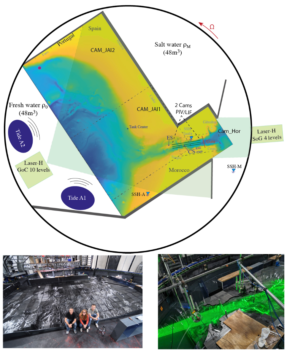
Figure 1 Sketch of the experimental setup with the topography position inside the Coriolis tank, the position of the tidal generators and the gate position for the lock-exchange baroclinic initial condition. Dashed lines indicate the horizontal and vertical views of the optical measurements and the positions of the lasers. The three green parallel lines in the strait represent the vertical sections for PIV/LIF measurements. Three capacitors measured the variation of the free surface at three positions in the Atlantic (SSH-A), in the Mediterranean (SSH-M) and at Tarifa (SSH-T). The dot off of Faro is a CTD used to detect the arrival of Mediterranean waters at the end of the topography. The bottom panels display an instantaneous picture of the topography installed within the Coriolis tank with a global view on the bathymetry of the Gulf of Cadiz (left) and an instantaneous image with horizontal laser prior to gate removal focused on the Strait viewed from the Spanish coast.

3.2 Dynamical forcings

3.2.1 Baroclinic flow

The initial condition for the baroclinic flow is the lock-exchange configuration, to spontaneously reproduces the equal exchange flow with the correct hydraulic controls. The duration of the experiment is then limited by the volumes of water that can be exchanged. This method does not allow to take into account the net barotropic transport of about 0.05 Sv towards the Mediterranean to compensate the excess of evaporation Soto-Navarro et al. (2010). Since it represents 1.5 %–2 % of the tidal barotropic oscillations, results will not be affected by this approximation.

The tank was divided in two equal volume compartments (with 5.5 m³ effectively available for the exchange flow) by a gate positioned within the strait (cf. Fig. 1, red strait line). The tank was filled simultaneously in both compartments up to a total depth of 65 cm (9.6 cm above CS) and put in anticlockwise rotation with a rotation period of T_c=124.8 s, as from the scaling given in Table 1. One reservoir was filled with saline water with density ρ_M, representing the Mediterranean Sea, the second with a lighter fluid of density ρ₀ corresponding to the Atlantic Ocean, both at the same temperature of ≈18° so that in the experiment the density is a function of salinity only. The density difference was kept constant with $\mathrm{\Delta }{\mathit{\rho }}_{\mathrm{0}}=\mathrm{19}(\pm \mathrm{1})$ kg m⁻³ in accord with the scaling given in Table 1. Considering an emptying speed U_g and the half-section at CS, the experimental duration was estimated to be about 30 min, corresponding roughly to $t/T_{\mathrm{c}}\sim \mathrm{15}$ rotational days.

At the start of the experiment following the gate removal, the flow through the strait undergoes through three regimes (Lawrence, 1990; Zhu and Lawrence, 2000; Negretti et al., 2007a): an initial unsteady phase in which the flow in each layer increases rapidly, a stationary regime called of maximum exchange and, finally, a sub-maximal exchange in which the flow decreases because no sufficient density difference is still present to maintain the initial hydrostatic pressure gradient. The useful phase for the experiment is the maximal exchange regime and this phase must be maintained long enough for the outflowing Mediterranean water to reach the end of the topography along the Portugal coast in geostrophic adjustment. During the maximum exchange phase, the strait is bounded by two hydraulic controls, preventing the changing boundary conditions of the two basins from influencing the flow at CS and keeping it stationary (Armi, 1986; Armi and Farmer, 1986; Lawrence, 1990, 1993; Zhu and Lawrence, 2000; Negretti et al., 2007b; Prastowo et al., 2006; Fouli and Zhu, 2011). Fig. 2a shows the time evolution of the flow speed (blue continuous line) in the salty layer at CS at 1.6 cm (40 m in the ocean) from the bottom, where a stationary, maximal exchange flow regime is rapidly reached, with an average velocity of 6.9 cm s⁻¹. The speed resulting from applying $G^{\mathrm{2}}=\mathrm{2}{U}_g^{\mathrm{2}}/\left(g^{\prime }{H}_{\mathrm{s}}\right)=\mathrm{1}$ corresponds to 6.8 cm s⁻¹. The figure also shows that the baroclinic experiment lasts at least 25 min (21.7 d for the ocean) during the stationary maximal exchange. The grey continuous line in Fig. 2a gives the salinity evolution from a CTD placed at the end of the topography ($-\mathrm{7.830}\mathit{°},\mathrm{36.840}\mathit{°}$) 1 cm (25 m in the ocean) from the bottom along the Portugal continental shelf (see Fig. 1). It shows that the first saline water is detected after 7 min after gate removal in the Strait (≈6 d in the ocean). This gives a stationary condition everywhere for $\mathrm{7}<T\left(\text{days}\right)<\mathrm{22}$.

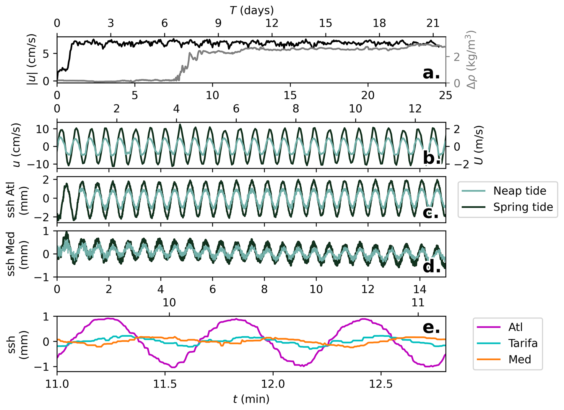
Figure 2 (a) Time evolution of the baroclinic velocity (black line) measured using an ADV at the CS summit within the Mediterranean layer 1.6 cm (40 m in the ocean) from the bottom, highlighting the rapid initial settling of the maximal exchange regime, which lasts up to 14 rotational days. The grey line is relative to a density measurement off of Faro (Portugal) along the continental shelf using a CTD-F probe 1 cm (25 m in the ocean) from the bottom, highlighting the time for the Mediterranean Outflow needed to reach the Portugal coast at the end of the topography, corresponding to roughly 6 rotational days. (b) Purely barotropic velocities measured with the ADV at the CS summit within the Mediterranean layer 2.6 cm (65 m in the ocean) from the bottom, being of maximum 10 cm s⁻¹ in the spring tide configuration (black lines), and half in the neap tide configuration (green lines), with the corresponding SSH anomalies in the Atlantic (c) and in the Mediterranean (d) basins. (e) Comparison of the SSH anomaly over three tidal cycles for the Atlantic (purple line), the Mediterranean (orange line) and at Tarifa (cyan line), highlighting a phase shift between the Atlantic basin and the Tarifa station for the tidal amplitude of 0.2T_tide. Experimental units (bottom-left), real ocean units (top-right).

3.2.2 Barotropic flow

The experimental parameter that has been varied in the experiments is the strength of the barotropic forcing: without tides (purely baroclinic flow) and stationary spring and neap tides. To reproduce tidal forcing, two different plungers A₁ and A₂ were both placed in the Atlantic basin (cf. Fig. 2), moving vertically and each displacing up to 80 L of water, at a frequency f_M2=35.77 s (12 h 25 min in the real ocean case), which corresponds to the frequency of the main tidal component in this region, i.e. the semi-diurnal tide M2 (Lafuente et al., 2015; Hilt et al., 2020; Roustan et al., 2023). The neap tide current has been reproduced using a single plunger with a given amplitude (A), whereas the spring tide was reproduced with a second plunger moving with the same amplitude A and frequency f_M2 as the first plunger. Further experiments have been performed also adding the modulation of the M2 component with the S2 component (corresponding to a 12 h period), in which case the plungers worked with a different amplitude and a different frequency (f_M2 and f_S2=34.56 s corresponding to 12 h in the real ocean). These measurements have been only used in Sect. 4.2.5 in the present paper.

The tide in the Strait of Gibraltar creates a barotropic current of the order of magnitude of 1 m s⁻¹ at CS during neap tide and up to twice during spring tide (Hilt et al., 2020; Roustan et al., 2023). The barotropic flow for both neap tide and spring tide conditions in the laboratory model are reported in Fig. 2b. The ADV (Acoustic Doppler Velocimetry, see Sect. 3.3) placed at CS at $z=-\mathrm{7.2}\mathrm{cm}$ from the free surface, measured an amplitude of 10 cm s⁻¹ for the purely barotropic velocity¹ in the spring tide configuration and 5 cm s⁻¹ in the neap tide configuration, which is in agreement with in situ measurements (Roustan et al., 2023) considering a velocity scale factor of 20 (cf. Table 1).

The barotropic speed is associated with a very low sea level (SSH) variation within the Strait and in the Mediterranean Sea. In the Gulf of Cadiz, on the other hand, the tidal amplitude can reach up to 1 m, but barotropic velocities are 10 times lower than those observed in the Strait.

An interesting feature of the Strait of Gibraltar is that the barotropic flow, responding to the standing-wave nature of the tidal sea level oscillation, heads west (tidal outflow) between low water and high water and heads east (tidal inflow) between high water and low water (Lafuente et al., 2015; Naranjo et al., 2015). This cannot be represented by our experimental set-up, in which an increase of sea level in the Atlantic corresponds to an eastward flow, and reversely during the SSH decrease.

The plungers can also reproduce the relative difference in SSH between the Atlantic and the Mediterranean basins, as their location in the western reservoir means that sea levels rise much less to the east of the strait than to the west. This is shown in Fig. 2c, d, in which the SSH anomalies due to spring tide (black curves) and neap tide (green curves) forcing are reported in the Atlantic (c) and in the Mediterranean (d). In the Atlantic basin, SSH variations are up to 2 mm for the spring tide forcing and half for the neap tide forcing, corresponding to 5 and 2.5 m in the real ocean. This is not in similarity with the real ocean since we have not respected similarity of the external Froude number. The variations in the Mediterranean are much smaller, reduced by a factor 2.5 with respect to the Atlantic ocean SSH variations, in accord with observations (Lafuente et al., 2015; Candela et al., 1990). Since we are interested here in the dynamics related to the barotropic/baroclinic flow rather that the effects of the SSH, the consequences of these differences on the dynamics with respect to the real ocean case have no impact on the generality of our results.

Note that when combining the baroclinic and barotropic forcings, a refinement of the plunger's amplitudes has been performed to match oceanic measurements, since the strength of the barotropic forcing leads to a different net baroclinic exchange flux across the Strait, as reported from observations. Indeed, previous authors (Bryden et al., 1994; Tsimplis and Bryden, 2000; García-Lafuente et al., 2002a; Morozov et al., 2002) reported that the strong interaction of the tidal forcing with the rough topography leads to non-linear interactions between the transport and the density interface location, making the tide to contribute to the exchange flow at subinertial scale, via eddy fluxes. We will show in Sect. 4.2.5 and 4.3 that in fact, the eddy fluxes contribution is negligible with respect to 3D topographical effects. Figure 2e displays a zoom on three tidal cycles of the Atlantic (violet), Mediterranean (orange) and at Tarifa (cyan) SSH, highlighting a phase shift between the Atlantic basin and the Tarifa station for the tidal amplitude of 0.2T_tide.

3.3 Measurements techniques

Measurements consisted in both intrusive and optical techniques, which are detailed below.

Three Acoustic Doppler Velocimetry (ADV, Vectrino, operating at 240 Hz), four 125 MicroScale Conductivity and Temperature Instrument (MSCTI, PME Vista, California, USA) and seven digital 4-electrode conductivity sensors (Endress Hauser Memosens CLS82E) devices were used to monitor the velocities and densities in several regions along the Spanish/Portugal continental shelf and in several channels within the Strait, at the exit of the Strait and in the Gulf of Cadiz channels (e.g. Majuan Banks, Gibraltar Channels, Cadiz and Guadalquivir Channels and Gil Eanes Furrow). Since this paper focuses on the dynamics of the Strait in which we used optical measurements techniques, the detailed map and a table with the exact positions of the intrusive devices is given in Bardoel et al. (2026) only. The free surface elevation anomaly (SSH) in both the Atlantic and Mediterranean basins and close to Tarifa were monitored throughout the experimental runs using highly precise interferometers with a precision of 10⁻² mm.

Optical measurements were made using PIV in both horizontal and vertical views, combined with Planar Laser Induced Fluorescence (PLIF) for the vertical views in some experiments.

The PIV set-up consisted of a light source, light-sheet optics, seeding particles, several cameras, and PCs equipped with a frame grabber and image acquisition software. Polyamide particles (Orgasol) with a mean diameter of 60 µm and a specific density of 1.022 kg m⁻³ were added to both salt and fresh water compartments as tracer material for the PIV measurements. The laser provided a continuous light source, with the beam passing through an optical lens with an angle of 75° that diverged the laser sheet in the area of interest for the horizontal measurements. An oscillating mirror was used to produce the laser sheet in the vertical views experiments.

A set of experiments to capture the horizontal velocity fields in the Strait was run with the laser sheet coming from the Mediterranean side, using a high-resolution SCMOS camera (PCO) with a resolution of 2560×2160 pixels. The laser system could be moved vertically along a linear axis to scan the water depth, yielding laser sheets for the Strait east of CS at five horizontal levels at $z=-\mathrm{0.065},-\mathrm{0.10},-\mathrm{0.14},-\mathrm{0.17},-\mathrm{0.20}$ m scanned twice. For each plane, 1400 images were taken at a frequency of 10 Hz, corresponding to 140 s measurement time for each plane.

Velocity fields were computed from PIV measurements using a cross-correlation PIV algorithm encoded with the UVMAT software (http://servforge.legi.grenoble-inp.fr/projects/soft-uvmat, last access: 2 February 2026). Each element of the resulting vector field represents an area of roughly 0.5 cm × 0.5 cm. The maximum instantaneous velocity error is estimated to be ≈3 %–5 %.

In the vertical configuration, the laser sheets coming from the top illuminated the full water column along the longitudinal section sketched in Fig. 3 in the Strait area, with an inclination of 18.5° North with respect to the East–West direction and passing through the CS summit. Images were recorded using a PCO camera at a frame rate of 50 Hz to capture the velocity fields. The laser system could be moved horizontally along a linear axis to scan the cross Strait section, yielding laser sheets at three parallel longitudinal transects at a distance of 5 and 6 cm from South to North respectively, relative to the middle transect passing through the CS summit, as sketched in Fig. 3b.

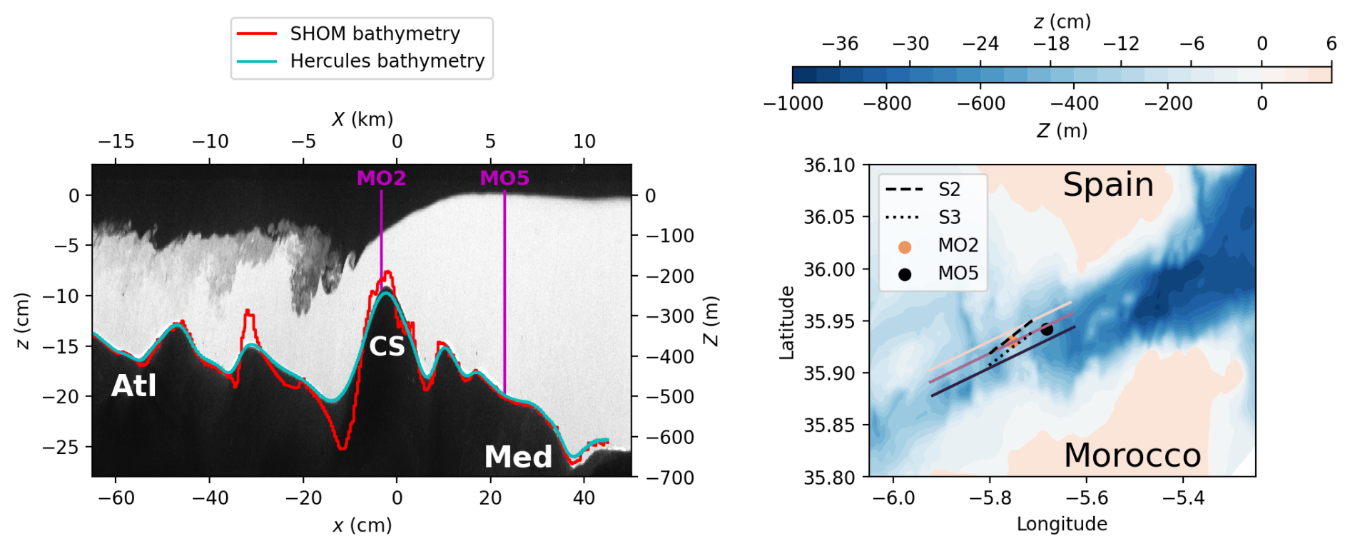
Figure 3 On the left, an instantaneous image of the laser plane during the experiment comparing the real topography (red line), the smoothed topography used in the present experiments (blue line) and the topography after calibration as registered on the camera images (black shadow), for the central transect. Vertical magenta lines gives the position closest to MO2 and MO5 moorings. On the right, sketch of the three transects considered for the PIV/LIF measurements (continuous lines), the middle one passing through the CS summit, and further southern and northern transects. The positions of the moorings MO2 and MO5 of the PROTEVS GIB2020 campaign (Bordois and Dumas, 2020) are given as well, along with the transects S2 and S3 (dashed and dotted lines, respectively), that will be used for comparison with the experimental data.

For some of the experiments in the vertical configuration, the PIV measurements were simultaneous to PLIF measurements, for which an identical high-resolution SCMOS camera (PCO) with the same lens as for PIV was used, at the same frame rate of 50 Hz, placed adjacently to the PIV camera and looking through the free surface with the same angle. An interferometer bandpass 532 nm for PIV and a high pass filter with cut-off 552 nm for PLIF were used to separate the emitted wavelengths for PIV and PLIF, respectively. The known initial concentration c₀ of Rhodamine 6G dye was then diluted and thoroughly mixed in the Mediterranean compartment, whereas Atlantic water was mixed with Ethanol for refractive-index matching to deliver the 2D instantaneous velocity and density fields. The detailed calibration procedure for the PLIF measurements is given in Appendix A. Rhodamine 6G was also used for flow visualization, especially to qualitatively track the pathways of the Mediterranean Outflow in the Gulf of Cadiz as used in Bardoel et al. (2026) and the interface in the Alboran Sea for internal waves, examined in Tassigny et al. (2026).

4 Dynamics in the Strait of Gibraltar

Since the flow is composed of a baroclinic (stationary) contribution, a periodic barotropic contribution and the fluctuating turbulent contribution, it is convenient to express the velocity and the density fields as the sum of the following three contributions (Hussain and Reynolds, 1970):

$$\begin{array}{}\text{(7)}& \begin{array}{rl}[u,\mathit{\rho }](x,z,t)& =[\stackrel{\mathrm{‾}}{u},\stackrel{\mathrm{‾}}{\mathit{\rho }}](x,z)+[\stackrel{\mathrm{̃}}{u},\stackrel{\mathrm{̃}}{\mathit{\rho }}](x,z,t)\\ & +[u^{\prime },{\mathit{\rho }}^{\prime }](x,z,t)\end{array}\end{array}$$

The mean flow $[\stackrel{\mathrm{‾}}{u},\stackrel{\mathrm{‾}}{\mathit{\rho }}]$ is computed as a time average over 7 tidal cycles.The tidal oscillating contribution is computed with the phase average operator:

$$\begin{array}{}\text{(8)}& {\displaystyle }[\stackrel{\mathrm{̃}}{u},\stackrel{\mathrm{̃}}{\mathit{\rho }}]\left(t\right)=\int \left(\right[u,\mathit{\rho }\left]\right(s)-[\overline{u},\overline{\mathit{\rho }}\left]\right)G(t-s)\mathrm{d}s\end{array}$$

where G is a Gaussian kernel with a standard deviation of 0.2 s (0.6 % of T_tide) and a period T_tide. The turbulent component $[u^{\prime },{\mathit{\rho }}^{\prime }]$ is obtained by subtracting these two averages to the raw signal.

In the following Sect. 4.1, we first present time averaged velocity and density fields ($\stackrel{\mathrm{‾}}{u}$, $\stackrel{\mathrm{‾}}{\mathit{\rho }}$), whereas the inflow and outflow dynamics during both spring tide and neap tide ($\stackrel{\mathrm{̃}}{u}$, $\stackrel{\mathrm{̃}}{\mathit{\rho }}$) are analyzed in Sect. 4.2.

In the following sections, some experimental results are directly compared with in situ observations obtained during the PROTEVS GIB20 campaign (Bordois and Dumas, 2020) conducted by SHOM (Service Hydrographique et Océanographique de la Marine, the French Naval Hydrographic and Oceanographic Service). This large-scale intensive survey covered the Strait of Gibraltar, the Bay of Cadiz, and the Alboran Sea during a strong (near-equinox) fortnightly tidal cycle in October 2020. In this study, we focus on a subset of measurements collected at moorings MO2 and MO5, which were equipped with Conductivity–Temperature–Depth (CTD) sensors used to reconstruct the vertical density field and an acoustic doppler current profiler. Data collected along transects S2 and S3 included velocity profiles measured with vessel-mounted Acoustic Doppler Current Profiler (VMADCP), conductivity and temperature profiles measured with moving vessel profiler as well as acoustic backscatter measurements. The instrumentation and their main characteristics are described in detail in Roustan et al. (2023). The locations of the moorings and transects are shown schematically in Fig. 3b.

4.1 Mean flow dynamics

4.1.1 Averaged velocity and density fields

Figure 4 presents characteristics of the mean velocity and density fields around CS averaged over seven tidal cycles during the stationary maximal exchange regime for the middle transect (cf. Fig. 3b) under three different tidal forcing scenarios: without tide (left column), neap tide (middle column), and spring tide (right column). The same for the northern and southern transects is presented in Figs. B1 and B2, respectively, given in the Appendix B. The arrows in the top panels represent the in-plane mean velocities. Note that the quiver plot is displayed with unequal vertical and horizontal scaling. Arrow angles are defined in data coordinates, so a velocity tangent to the seabed appears as an arrow tangent to the bottom. Because the figures are vertically stretched for readability, preserving geometric angles would misrepresent the actual flow direction. Arrow length is hence determined solely by the in-plane speed as commonly done in the literature. The colormap highlights the mean dimensionless ratio of density differences ${\mathit{\rho }}^{*}\equiv \mathrm{\Delta }\mathit{\rho }/\mathrm{\Delta }{\mathit{\rho }}_{\mathrm{0}}=(\stackrel{\mathrm{‾}}{\mathit{\rho }}-{\mathit{\rho }}_{\mathrm{0}})/({\mathit{\rho }}_{\mathrm{M}}-{\mathit{\rho }}_{\mathrm{0}})$, with $\stackrel{\mathrm{‾}}{\mathit{\rho }}$ being the averaged density over the seven considered tidal cycles. Comparison of the top panels indicates that increasing tidal forcing leads to a thickening of the mixed layer on both sides of the sill. This effect is partly due to the time-averaging procedure, as the interface oscillates more strongly with increasing tidal amplitude, and partly due to enhanced mixing associated with stronger tides, as will be shown in Sect. 4.2, where tidal averages corresponding to maximum out- and inflow are presented.

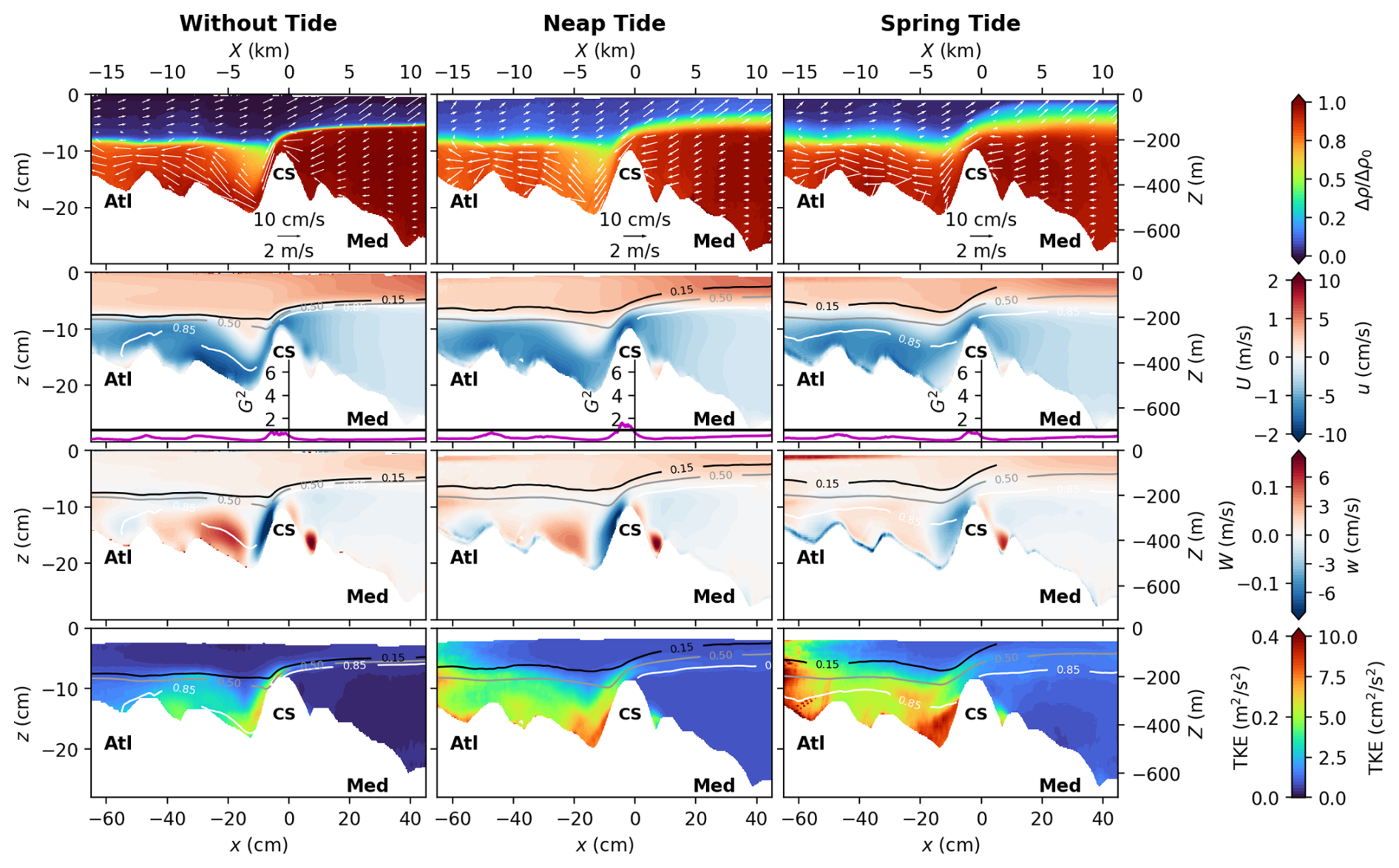
Figure 4 Mean flow characteristics for the middle transect passing through the CS summit (cf. Fig. 3b), for the three tidal forcings: without tide, neap tide, and spring tide from left to right. The x axis represents the along-transect coordinate, being positive toward the east. The first row displays the mean dimensionless ratio of density differences ${\mathit{\rho }}^{*}\equiv \mathrm{\Delta }\mathit{\rho }/\mathrm{\Delta }{\mathit{\rho }}_{\mathrm{0}}=\stackrel{\mathrm{‾}}{\mathit{\rho }}-{\mathit{\rho }}_{\mathrm{0}}/({\mathit{\rho }}_{\mathrm{M}}-{\mathit{\rho }}_{\mathrm{0}})$, with $\stackrel{\mathrm{‾}}{\mathit{\rho }}$ being the averaged density over the seven considered tidal cycles. Averaged in-plane velocities $(\stackrel{\mathrm{‾}}{u},\stackrel{\mathrm{‾}}{w})$ are given by the white arrows. Note that the quiver plot is displayed with unequal vertical and horizontal scaling. Arrow angles are defined in data coordinates and the arrow length is determined solely by the in-plane speed. The second and third rows panels display the mean horizontal $\stackrel{\mathrm{‾}}{u}$ and vertical $\stackrel{\mathrm{‾}}{w}$ velocities, respectively, superposed with the $\mathrm{\Delta }\stackrel{\mathrm{‾}}{\mathit{\rho }}/\mathrm{\Delta }{\mathit{\rho }}_{\mathrm{0}}=\mathrm{0}$.15, 0.5, and 0.85 (black, grey, and white lines respectively). In between, the time-averaged composite Froude number G² is displayed as a purple line. The last row panels display the turbulent kinetic energy $\mathrm{TKE}=(\stackrel{\mathrm{‾}}{u^{\prime \mathrm{2}}}+\stackrel{\mathrm{‾}}{w^{\prime \mathrm{2}}})/\mathrm{2}$. Experimental units (bottom-left), real ocean units (top-right).

The mean density fields ρ^* shown in the top panels of Fig. 4 reveal that the time-averaged density is overall more diluted, by approximately (0.15–0.2)ρ^* east of the CS, when tides are present, particularly during spring tide, compared with the purely baroclinic case (left panel). Direct comparison of the mean dimensionless ratio of density differences ρ^* at different position in the along-strait direction for the three tidal forcings is given in the Appendix C. This will be also further discussed in Sect. 4.2.

Also, it appears that Mediterranean waters are more diluted (of about 0.3ρ^*) west of CS in neap tide compared to spring tide conditions, an aspect which will be further discussed in Sect. 4.2. These observations are also applicable in the case of the northern (Fig. B1) and southern (Fig. B2) transects given in the Appendix.

In the absence of tides, the surface of maximum vertical gradient of the along-strait velocity h_u closely follows the pycnocline h_p on the eastern side of the sill, defined as the iso-density lines with ${\mathit{\rho }}^{*}=\mathrm{1}/\mathrm{2}$, and illustrated by the grey line presented in the middle rows panels of Fig. 4. The alignment between h_u and h_p is disrupted when tidal forcing is introduced, suggesting that tides generate entrainment of Mediterranean water to the west of CS. This aspect is further discussed in Sect. 4.2 as well. Along-strait velocities u averaged over the tidal cycles weaken west of CS when the tide is applied, compared to the purely baroclinic case (see second row panels of Fig. 4).

The abrupt downward plunge of the pycnocline and the increased thickness of the mixed layer west of CS suggests the presence of an internal hydraulic jump for all tidal conditions. This is supported by the strong vertical velocity $\stackrel{\mathrm{‾}}{w}$ change in the third row panels of Fig. 4 observed at the same location. When the tidal amplitude increases in spring tide conditions, the positive/negative maxima of the vertical velocity descend. This can be understood considering that the differences between inflow and outflow are more pronounced during spring tide as compared to neap tide: during outflow, the Mediterranean waters are advected further downstream and the internal hydraulic jump oscillates west of CS with the tidal phase and disappears even during inflow, such that the averaged velocity fields are homogenized over the entire considered field on the west of CS. During neap tide instead, the internal hydraulic jump is stably localized close to the western flank of the sill and persists longer during the tidal cycle, even during part of the inflow. This will be further discussed in the following Sect. 4.2 below.

The local composite Froude number G² provides insights into the local criticality of the flow. To compute the composite Froude number, a two-dimensional two-layer model has been defined, with the interface defined as the pycnocline ${\mathit{\rho }}^{*}=\mathrm{1}/\mathrm{2}$, each layer of mean thickness ${\stackrel{\mathrm{‾}}{h}}_i$ characterized by a constant along-strait mean velocity ${\stackrel{\mathrm{‾}}{u}}_i$ and a local value for g^′ (see Appendix E), i.e.

$$\begin{array}{}\text{(9)}& {\displaystyle }{G}^{\mathrm{2}}={\displaystyle \frac{{\stackrel{\mathrm{‾}}{u}}_{\mathrm{1}}^{\mathrm{2}}}{g^{\prime }{\stackrel{\mathrm{‾}}{h}}_{\mathrm{1}}}}+{\displaystyle \frac{{\stackrel{\mathrm{‾}}{u}}_{\mathrm{2}}^{\mathrm{2}}}{g^{\prime }{\stackrel{\mathrm{‾}}{h}}_{\mathrm{2}}}}.\end{array}$$

The validity of these assumptions is still largely debated in the community, as several studies emphasize that the mixed layer plays an important role in controlling exchange-flow dynamics (e.g. Bray et al., 1995; Sannino et al., 2007). In the Appendix E, we present and discuss different ways of computing the composite Froude number including three-layers models. Since results do not present particularly relevant differences, we will use the classical two-layer model with the pycnocline ${\mathit{\rho }}^{*}=\mathrm{1}/\mathrm{2}$ defined as interface and using a local g^′ instead of the initial constant value of $g_{\mathrm{0}}^{\prime }$, which are more consistent with the hypothesis under which the composite Froude number is derived.

Mathematically, a condition of G²⩾1 is necessary for the development of a stationary shock such as hydraulic jumps (Armi and Farmer, 1985; Sánchez-Garrido et al., 2011). However, the condition G²⩾1 alone does not guarantee hydraulic control at a cross-strait section (Pratt, 2008). The analysis presented here remains local and restricted to each transect and focuses on the potential for the development of localized shocks.

The composite Froude number G², shown in Fig. 4 below the second row panels as a purple line, exhibits averaged values below unity everywhere and approaches unity at CS in all transects. Note that some uncertainty is present in the determination of G since velocity values close to the bottom boundary and the free surface are subject to more uncertainty and in some transects or tide conditions the upper layer velocities are sometimes missing close to the free surface. Hence, we expect our computed G² being rather underestimated. These effects combined with the three-dimensional nature of the flow, which calls for a global criticality of the flow to be defined (Pratt, 2008), can explain the failure of the computed composite Froude number to capture regions in which G²⩾1 in the average. Note also that the presented values are a total temporal average: when computing the internal Froude number during a tidal cycle, values of G²⩾1 are captured, as it will be shown further below in Sect. 4.2. The same conclusions are also valid for the northern and southern transects given in Figs. B1 and B2, respectively, that are given in the Appendix.

The bottom panels of Fig. 4 (and Figs. B1 and B2 for the northern and southern transects given in the Appendix) report the turbulent kinetic energy ($\mathrm{TKE}=(\stackrel{\mathrm{‾}}{u^{\prime \mathrm{2}}}+\stackrel{\mathrm{‾}}{w^{\prime \mathrm{2}}})/\mathrm{2}$), which interestingly appears to be highest close to the bottom boundaries. The intensity of the TKE also increases with increasing tidal forcing and appears to be linked to the bottom boundary-layer detachment on the west side of CS and the formation of a recirculation area. In comparison, the TKE between the two layers at the interface of Mediterranean and Atlantic waters is roughly half as strong. Moreover, since the detachment appears only when the tidal forcing is present, as shown from the second row panels for the velocity u. In the purely baroclinic case, high TKE values at the interface are observed at the onset of the descent. Further downstream, the interface becomes indistinguishable due to the development of the hydraulic jump, where TKE values increase. It should be noted that, due to the larger aspect ratio used in the experiments, the TKE is not strictly in similarity to that in the real ocean. Since the characteristic velocity scales are U in the horizontal and $(H/L)U$ in the vertical, the relative contribution of vertical velocity fluctuations (w^′) to the TKE is enhanced in the experimental configuration, potentially leading to elevated turbulence levels. Nevertheless, because the vertical contribution remains smaller in magnitude than the horizontal one, the overall order of magnitude of the TKE is preserved.

An overview of the averaged flow over four tidal cycles in the Strait at different depths (from −142.5 to −365 m) is shown in Fig. 5, for the considered three tidal conditions (without tide, neap tide, and spring tide from left to right). Horizontal velocities are displayed by the arrows, whereas the color fields indicate the relative vertical vorticity component ω, normalized by the Coriolis parameter f.

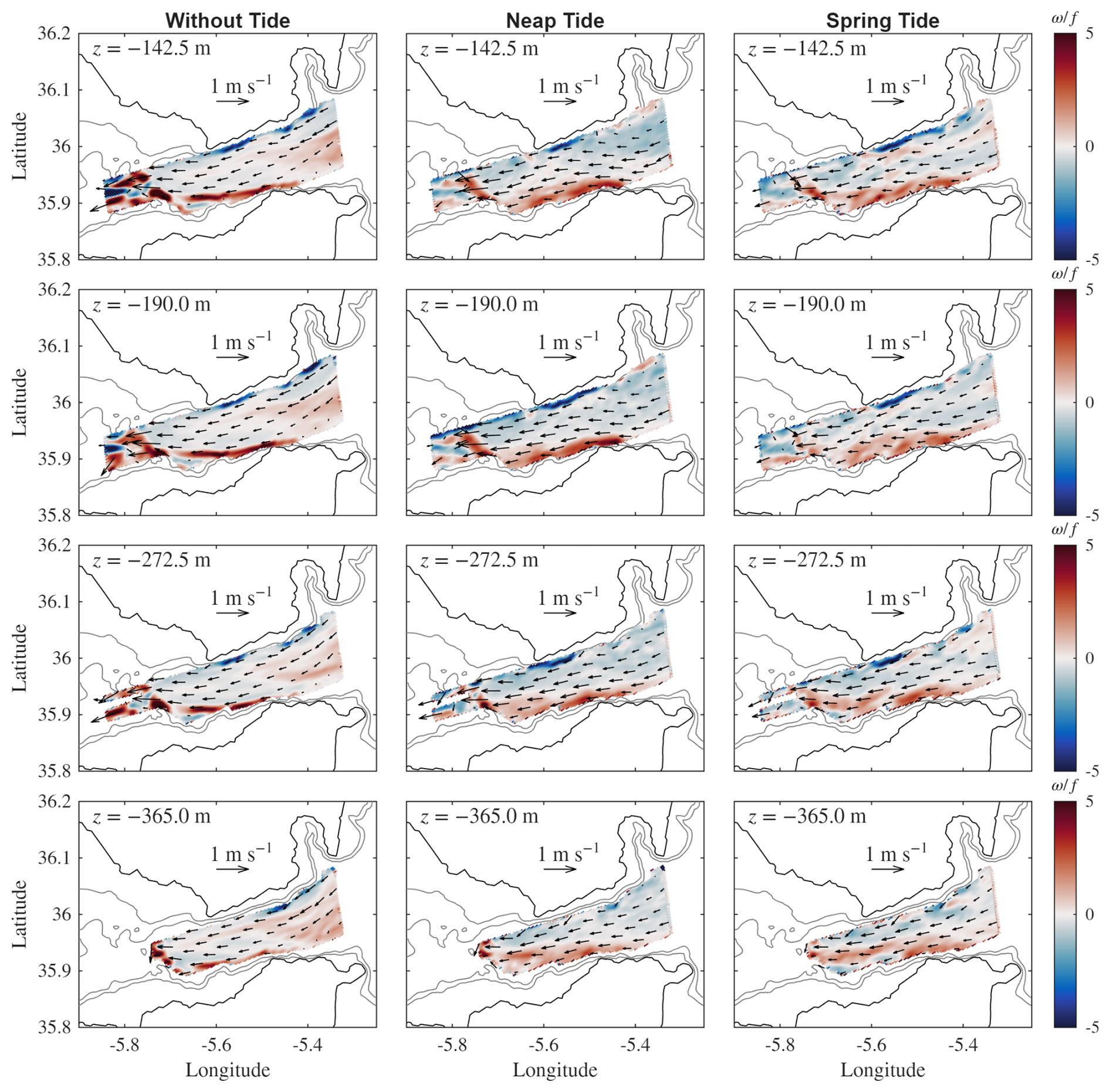
Figure 5 Averaged (over four tidal cycles) in-plane horizontal velocities with superposed relative vorticity field (colormap) in the Strait of Gibraltar at various depths for the three tidal forcings: without tide (left column), neap tide (center column), and spring tide (right column).

Overall, the flow is channeled toward the Tarifa narrow increasing the velocity while approaching CS, with similar velocity amplitudes in all depths except the deepest one at $z=-\mathrm{365}$ m, for all three tidal conditions. Velocities are overall smaller in the purely baroclinic case. From the colored vorticity plots, it appears again that the highest values are reported along the coastline where strong changes of bathymetry (depth) appear, highlighted by the grey contour lines in Fig. 5, and in the region where the hydraulic jump appears immediately downstream of CS. When approaching the bottom, the vertical vorticity is increasing overall within the displayed field especially for the spring tide conditions (left column) because of the increasing shear due to the the bottom topography and flow detachment.

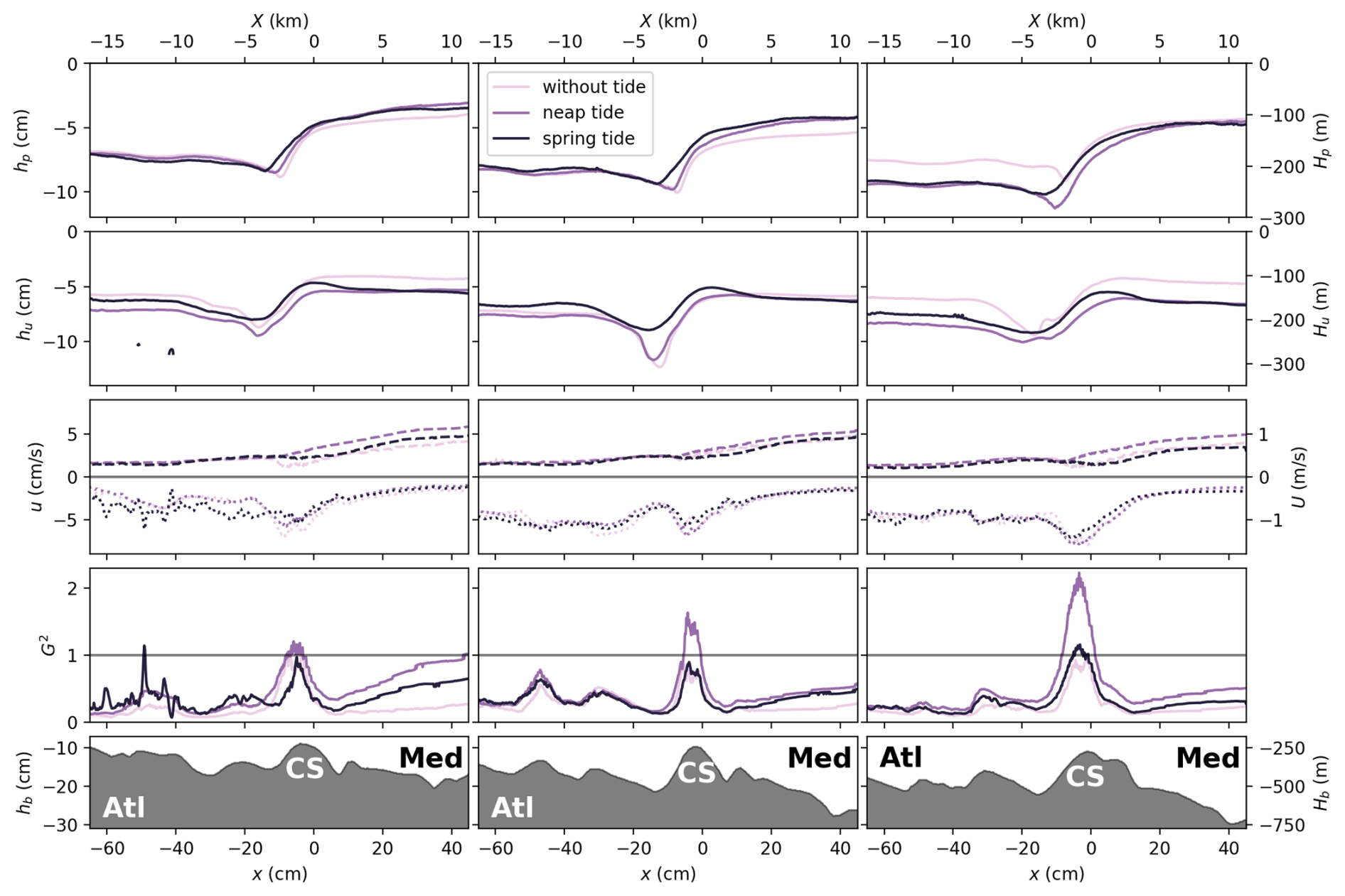
Figure 6 Two-layer time-averaged (over seven tidal cycles) flow characteristics at CS for the planes (from left to right: northern, middle and southern transects) for the three tidal forcing. From top to bottom: pycnocline depth h_p; surface of maximum vertical gradient of along-strait velocity h_u; vertically integrated along-strait velocity u for the Mediterranean (dotted lines) and Atlantic (dashed lines) layers; two layer composite Froude number G²; bathymetry. Experimental units (bottom-left), real ocean units (top-right).

4.1.2 Mean flow characteristics

The vertically averaged two-layer flow characteristics are summarized in Fig. 6 for the three tidal configurations and for the three transects: the left column corresponds to the southern transect, the central column to the middle transect, and the right column to the northern transect (cf. Fig. 3b).

The first row of the figure presents the pycnocline depth h_p defined as ${\mathit{\rho }}^{*}=\mathrm{1}/\mathrm{2}$. The pycnocline depth h_p shows minimal variation with changes in tidal forcing. In the northern plane, it remains essentially unchanged regardless of the tidal conditions. In the central plane, the tides cause a slight elevation of the pycnocline on the eastern side of CS, likely due to the thickening of the mixed layer, as predicted by hydraulic theory. This depth increase has been also reported in the numerical simulations of Sannino et al. (2007) and in observations Roustan et al. (2023). On the western side, the downward plunge of the pycnocline is less pronounced for spring tide conditions, likely as a result of the detachment of the Mediterranean waters from the bottom boundary during outflow. The surface of maximum vertical gradient of the along-strait velocity h_u exhibits limited sensitivity to tidal forcing as well, except near the sill where it becomes slightly shallower for spring tide, again likely linked to the boundary-layer detachment occurring during outflow. The third row panels of Fig. 6 shows the vertically averaged horizontal velocities in both the Atlantic (dashed lines) and in the Mediterranean (dotted lines) layers. Very little difference in these averaged values is reported for the different tidal conditions, except of lower values for the purely baroclinic case, as already reported in the literature (Roustan et al., 2023; Wesson and Gregg, 1994) and observed in the previous Fig. 5. In the Atlantic layer, velocities are increasing when moving toward the East due to the decreasing pycnocline depth and are nearby constant in all three sections for $x>\approx \mathrm{30}$ cm (≈7 km west of CS). In the Mediterranean layer velocities are increasing when moving to the West, reaching the highest values at CS, and then decreasing to a nearby constant value after the flow re-adjustemnt with the internal hydraulic jump for $x>\approx \mathrm{30}$ cm (≈7 km west of CS).

The local composite Froude number G² computed from Eq. (9) and shown in the following row panels, remains subcritical throughout the sections as already mentioned above, but exhibits a noticeable increase approaching the sill location. The maximum value of G² is up to 50 % higher during neap tide compared to the spring tide condition with exception of the northern transect where values remain similar for all tidal conditions. A local increase in G² is also reported in correspondence of other topographical features at $x=-\mathrm{30}$ and $x=-\mathrm{45}\mathrm{cm}$ (corresponding to −7.5 and −11.25 km in the real ocean) West of CS, where other hydraulic controls have been suggested by previous authors (Wesson and Gregg, 1994; Izquierdo et al., 2001; Hilt et al., 2020; Roustan et al., 2023). The criticality of the flow varying with the tidal phase is further discussed in the following section.

4.2 Dynamics in the tidal average

4.2.1 Horizontal fields

Figure 7 displays the in-plane horizontal velocities averaged over the four measured tidal cycles at the given phase with superposed relative vorticity field (colormap). We see that during inflow, the flow is arrested and slightly reversed within the Strait at this depth ($z=-\mathrm{190}$ m) and is clearly reversed during spring tide. The mean flow is directed following the continental shelf and influenced by the Coriolis force, resulting in canalizing the flow toward the North and the Spanish coast. We also see that very high values of relative vorticity (5 to 10 times the Coriolis frequency f) are concentrated along the coasts in proximity of the continental shelf characterized by strong depth gradients. Generally, during outflow and high water slack (the top row panels) the northern coastline is characterized by negative relative vorticity values, whereas the southern coastline is characterized by positive relative vorticity. During inflow and low water slack (latter two row panels) positive relative vorticity dominates overall. Also, during low water slack, bands of positive and negative vorticity are present just east of CS, possibly suggesting the presence of internal waves.

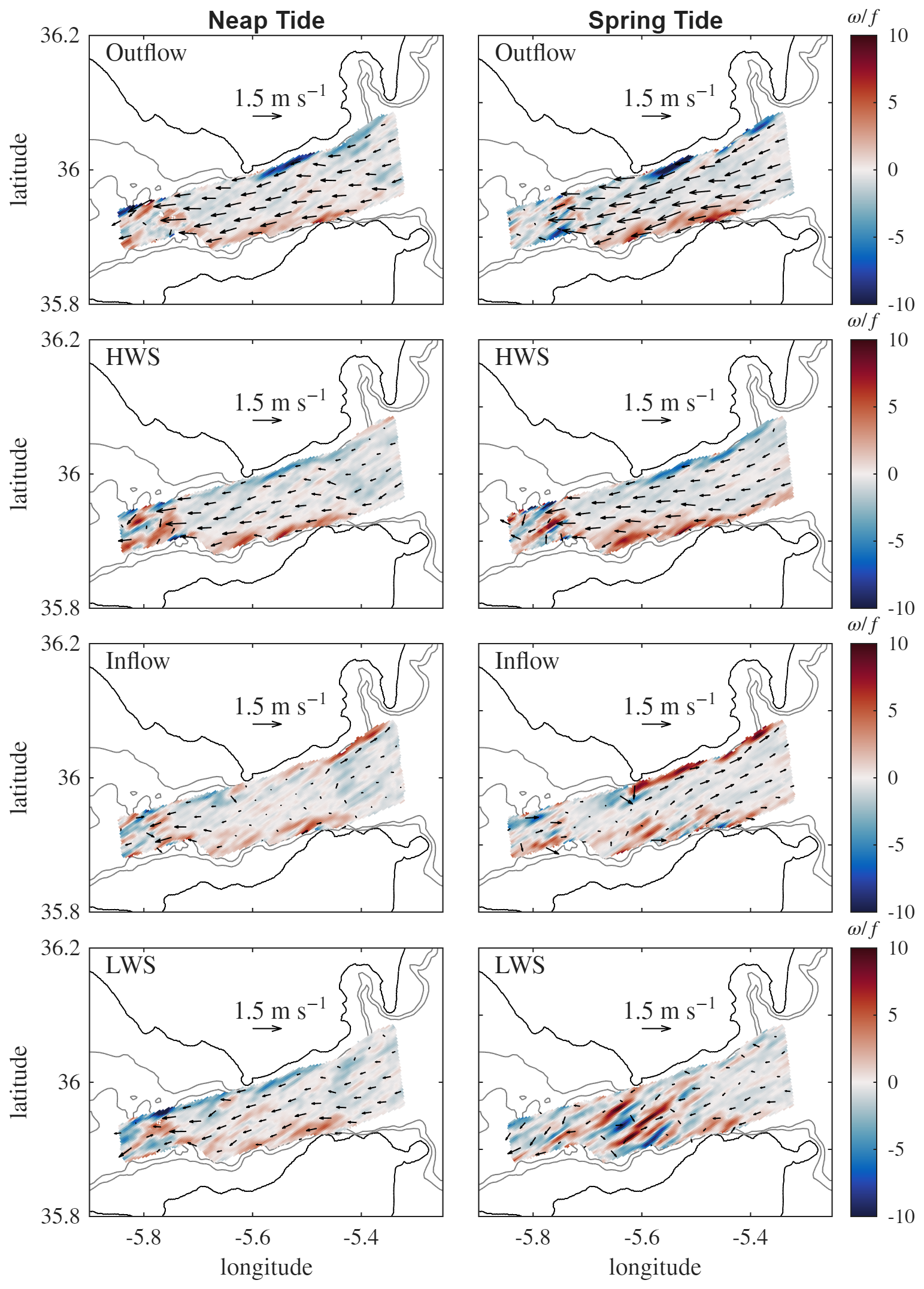
Figure 7 Averaged in-plane horizontal velocities over the four measured tidal cycles at the given phase with superposed relative vorticity field (colormap) in the Strait of Gibraltar at $z=-\mathrm{190}\mathrm{m}$ for neap tide (left column) and spring tide (right column) conditions, at four tidal phases corresponding to outflow (first row), high water slack (HWS, second row), inflow (third row), and low water slack (LWS, fourth row).

4.2.2 Inflow, outflow and slack dynamics

Similar to the panels in Fig. 4 presented in the previous section, Fig. 8 shows the results from simultaneous velocity and density measurements, averaged over the seven measured tidal cycles at maximum inflow (first and second rows) and maximum outflow (third and fourth rows) for both neap tide and spring tide conditions. Here, we focus on the middle transect only.

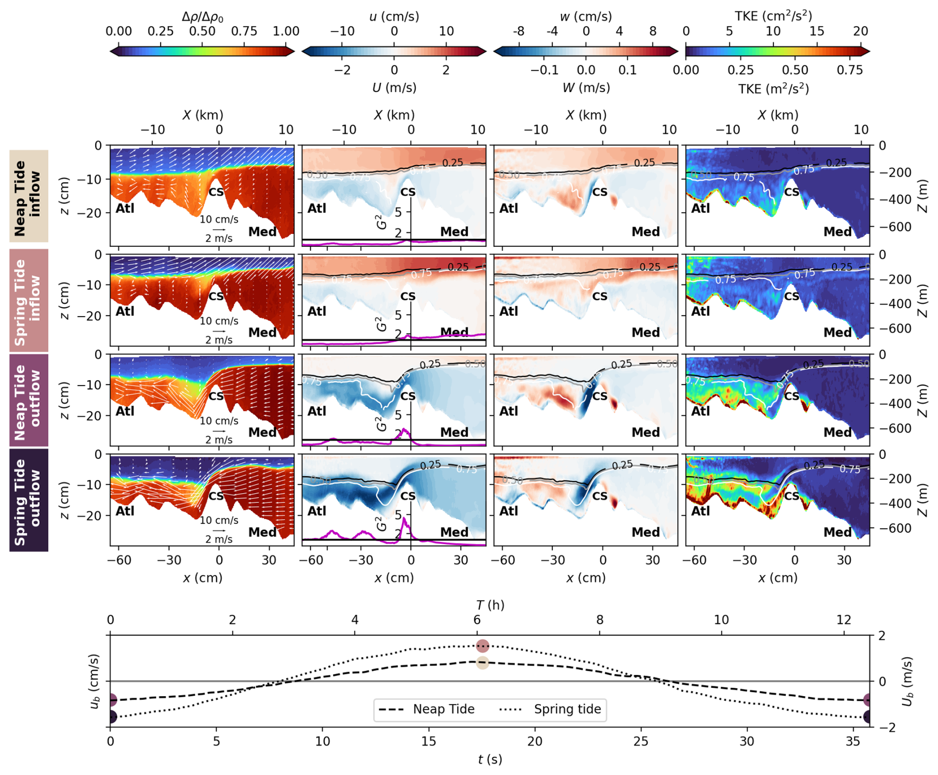
Figure 8 Mean flow characteristics for the middle transect passing through the CS summit (cf. Fig. 3b), for maximum inflow (first two row panels) and maximum outflow (last two row panels) for both neap tide and spring tide conditions. The x axis represents the along-transect coordinate, being positive toward the east. The first column displays the mean density with the averaged velocities $(\stackrel{\mathrm{‾}}{u},\stackrel{\mathrm{‾}}{w})$ (white arrows). The second and third columns panels display the mean horizontal u and vertical w velocities, respectively, superposed with the $\mathrm{\Delta }\mathit{\rho }/\mathrm{\Delta }{\mathit{\rho }}_{\mathrm{0}}=\mathrm{0.15}$, 0.5, and 0.85 (black, grey, and white lines respectively). The composite Froude number G² is displayed as a purple line below the along-strait velocity u panels. The last column panels display the turbulent kinetic energy $\mathrm{TKE}=(\stackrel{\mathrm{‾}}{u^{\prime \mathrm{2}}}+\stackrel{\mathrm{‾}}{w^{\prime \mathrm{2}}})/\mathrm{2}$. The bottom panel indicates the variation of the depth integrated barotropic velocity at CS over a tidal cycle with the dots indicating the maximum inflow and outflow corresponding to the above panels for neap and spring tides. Experimental units (bottom-left), real ocean units (top-right).

The density fields displayed in the left panels show that during both maximum inflow and outflow, dilution is enhanced under neap tide conditions on both sides of the sill, consistent with the total averaged fields in Fig. 4, except during the spring tide maximum outflow, where the strong barotropic tide produces slightly greater dilution $\approx \mathrm{0.1}{\mathit{\rho }}^{*}$ east of the sill.

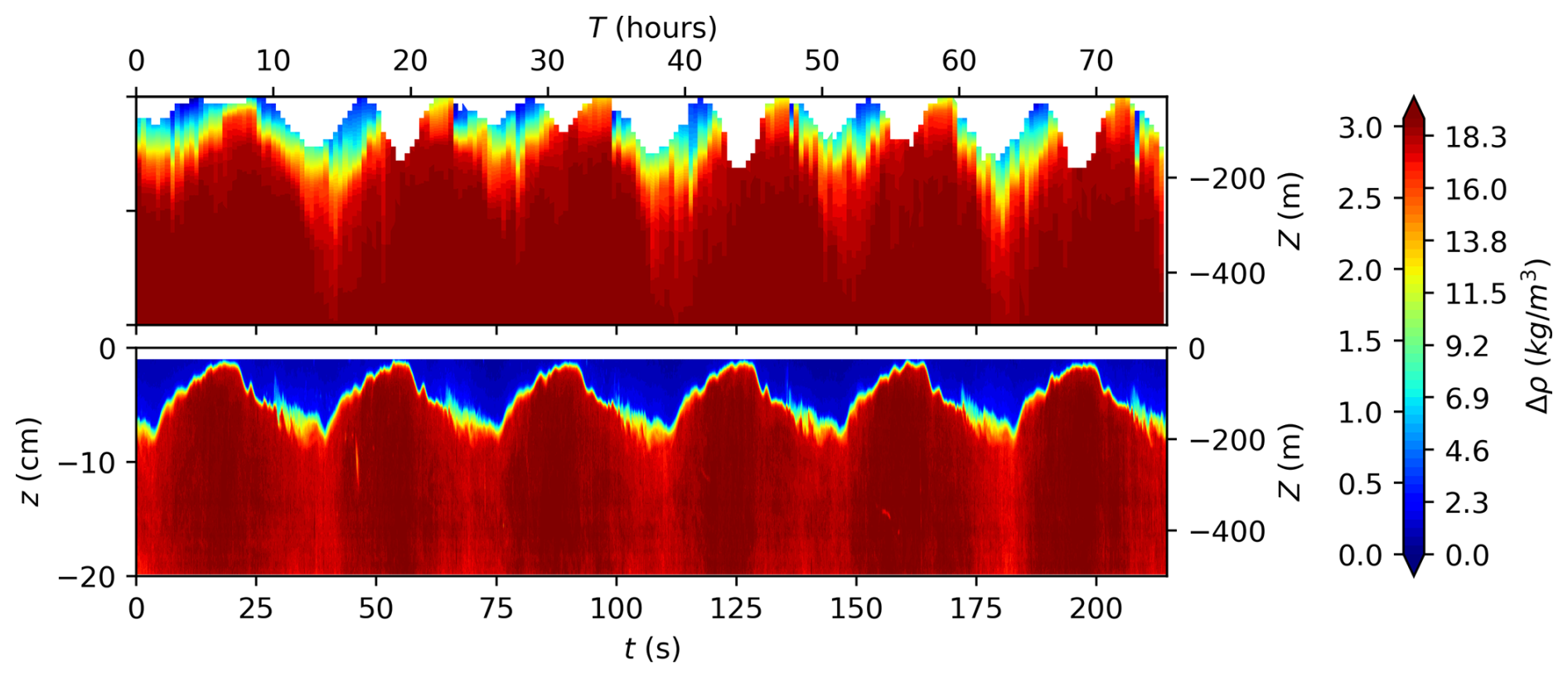
Figure 9 Hovmöller diagram at the position correspondent to MO5 mooring in the observational campaign GIB2020 displaying the relative density (left colorbar values: real ocean; right colorbar values: experiments) for the observational (top panel) and the experimental data of the experiment (bottom panels). A tidal variation of the order of $(\mathrm{0.15}-\mathrm{0.2}){\mathit{\rho }}^{*}$ in the full water column is evident in both panels.

A closer inspection, presented in Fig. 9, demonstrates that tidal forcing is capable of advecting the full water column down to 500 m of mixed waters east of CS during spring tide, with oscillations of the density ratio as a function of the tidal phase of the order of $(\mathrm{0.15}-\mathrm{0.2}){\mathit{\rho }}^{*}$. Since in the experiment we do not have different density components in the Mediterranean and in the Atlantic waters, in the experiment the whole Mediterranean layer is well mixed from the bottom to the interface with clearer differences between inflow and outflow. A direct comparison between our measurements at the MO5 mooring and the in situ observations from the PROTEVS GIB20 field experiment confirms the presence of the same tide-phase-dependent oscillations and the full-depth density ratio oscillation east of the sill. A pronounced thickening of the pycnocline is also evident when tidal forcing is applied, compared with the purely baroclinic case in Fig. 4.

During maximum neap tide inflow, examination of both the density (left panels) and velocity fields (further right panels) shows that the Mediterranean flow can still overflow the sill, forming a thin layer that is spilling down the western flank of the sill. In contrast, under maximum spring tide inflow, the Mediterranean Outflow is blocked. The internal hydraulic jump disappears for both neap tide and spring tide maximum inflow conditions, as indicated by the purple line representing the composite Froude number G² below the along-strait velocity field. Note that now G² is computed taking into account the contribution from the mean and the tidal flow, i.e.:

$$\begin{array}{}\text{(10)}& {\displaystyle }{G}^{\mathrm{2}}={\displaystyle \frac{({\stackrel{\mathrm{‾}}{u}}_{\mathrm{1}}+{\stackrel{\mathrm{̃}}{u}}_{\mathrm{1}}{)}^{\mathrm{2}}}{g^{\prime }({\stackrel{\mathrm{‾}}{h}}_{\mathrm{1}}+{\stackrel{\mathrm{̃}}{h}}_{\mathrm{1}})}}+{\displaystyle \frac{({\stackrel{\mathrm{‾}}{u}}_{\mathrm{2}}+{\stackrel{\mathrm{̃}}{u}}_{\mathrm{2}}{)}^{\mathrm{2}}}{g^{\prime }({\stackrel{\mathrm{‾}}{h}}_{\mathrm{2}}+{\stackrel{\mathrm{̃}}{h}}_{\mathrm{2}})}}.\end{array}$$

The hydraulic control that forms above CS during the outflow phase is distinct from the control that develops during inflow to the east of the sill, in the direction permitted for internal wave propagation. The control at CS prevents the eastward propagation of internal waves, whereas the control located to the east blocks westward propagation. When the control at CS is subsequently relaxed, the internal hydraulic jump propagates eastward, potentially contributing to the generation of internal solitary waves. This behavior is more clearly illustrated in the slack-water dynamics presented below and in the Hovmöller diagram of G² shown in Fig. 14. A detailed discussion of this process is provided in a separate study focusing on internal solitary wave generation (Tassigny et al., 2026).

TKE values presented in the rightmost panels of Fig. 8 are markedly reduced during maximum inflow for both neap tide and spring tide conditions compared with those in the total averages of Fig. 4. However, under neap tide conditions, since Mediterranean waters still pass over the sill, the strong shear in the thin Mediterranean vein close to the bottom boundary continue to generate localized moderate TKE.

During maximum outflow, very high TKE values are observed, concentrated in the bottom boundary layers west of the sill, with approximately half those values occurring along the sheared layer between the Mediterranean and Atlantic waters. The second-column panels suggest an offset between the pycnocline and the region of maximum velocity shear west of CS, particularly during spring tide. This will be further discussed below with Fig. 11 and in the Appendix D.

The hydraulic jump west of CS is characterized by an abrupt reversal in vertical velocity, transitioning from strongly negative to strongly positive values over a short distance. Consequently, the vertical velocity field provides a clear indicator of the location and intensity of the internal hydraulic jump. The internal hydraulic jump is evident at the sill for both neap tide and spring tide maximum outflow conditions, along with two additional control points farther downstream (to the west), more pronounced during spring tide. Our observations show that during neap tides, the vertical velocity attains higher maximum and minimum values within a confined region west of the sill. In contrast, during spring tides, the vertical velocity extremes are lower in magnitude but spread over a broader area. This behavior indicates that the hydraulic jump is displaced farther west during spring tides, whereas it remains confined to a more restricted region closer to the western flank of CS during neap tides.

A particularly noteworthy feature, previously visible in the total averaged along-strait velocity fields of Fig. 4 but now more clearly defined, is the region of weak or even positive velocities on the western flank of the sill, especially during spring tide outflow conditions. This pattern indicates that the Mediterranean vein detaches from the bottom boundary, which may be due to an adverse pressure gradient generated by the barotropic flow during outflow in the divergent region west of the CS. This divergent pressure field can become sufficiently strong to overcome the opposing baroclinic pressure gradient of the gravity current. This mechanism, which accounts for the elevated TKE values observed in the bottom boundary layers during outflow (see right column panels), is further examined in the following Sect. 4.2.3.

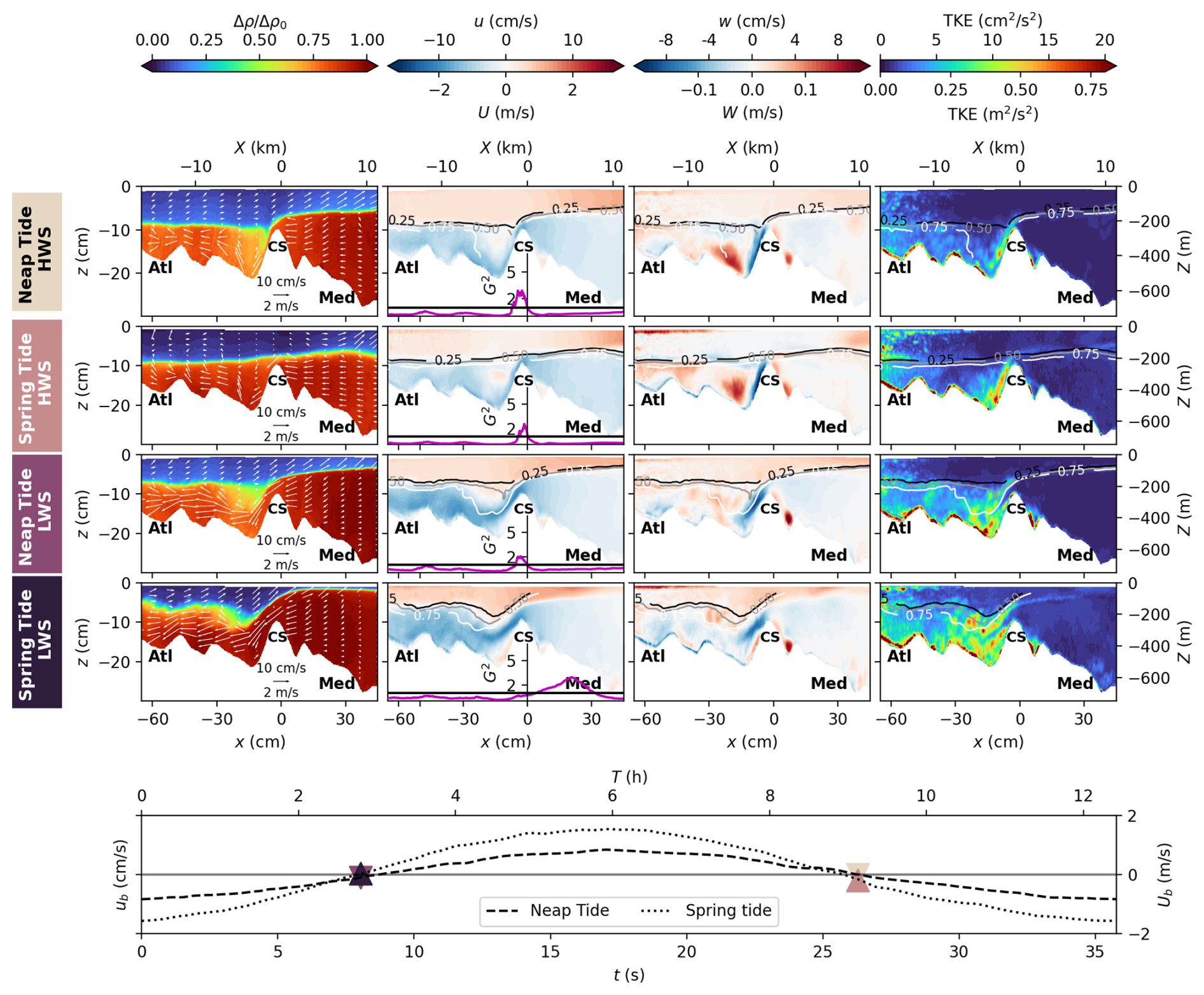
Figure 10 Same as in Fig. 8 but for the slack dynamics: high water slack (HWS) and low water slack (LWS).

Figure 10 presents the dynamics at high-water slack (top panels) and low-water slack (bottom panels) for both neap tide and spring tide conditions. Overall, it can be seen that even at these tidal phases, neap tide conditions produce stronger dilution of Mediterranean waters west of the CS compared with spring tide, with a difference of roughly 0.2ρ^*. East of the sill, the high-water slack exhibits about 0.1ρ^* greater dilution overall than the low-water slack, with mean dilution values of approximately 0.8ρ^* and 0.9ρ^*, respectively.

During high-water slack, a thin layer of Mediterranean water continues to spill down the western flank of the sill (see along-strait velocity fields), while part of this flow forms a recirculation cell particularly evident under neap tide conditions in the first panel of Fig. 10 and in the along-strait velocity fields of the second-column panels, where a circular region of positive velocity appears. Similar behavior has been observed in situ in Figs. 9b and 12 of Roustan et al. (2023), who reported large overturns along the slope, suggesting a reversal of the Mediterranean outflow acting as a strong gravity current, in addition to the shear instabilities in the interfacial mixed layer previously described.

An internal hydraulic control, indicated by the composite Froude number (G²>1), is present at the sill for both neap tide and spring tide conditions during high-water slack, with an internal hydraulic jump farther west, as shown by the strong positive and negative vertical velocities in the third-column panels. The thin layer flowing along the western boundary of the sill is responsible for the high TKE values observed there (see first panels of the right column).

During high-water slack, a decorrelation between the pycnocline and the region of maximum velocity shear is visible west of CS and up to x=20 cm (5 km in the real ocean) in the second-column panels of Fig. 10, for both spring tide and neap tide conditions, even if less marked in this latter case (see also Fig. 11). The same holds true during low-water slack.

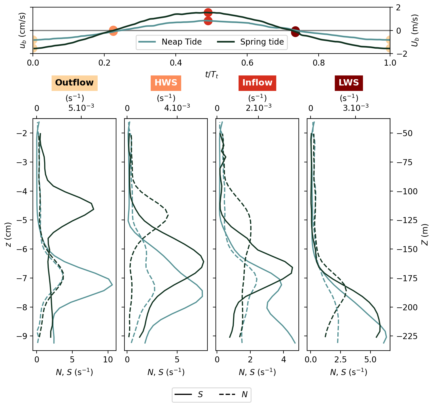
Figure 11 Vertical profiles of shear (full lines) and Brunt-Väisälä frequency (dashed lines) (at CS) corresponding to the MO2 mooring during maximum outflow (first column), high waters slack (second column), maximum inflow (third column) and low water slack (fourth column) for neap tide (green lines) and spring tide (black lines) forcing.

As already reported previously for the maximum inflow and outflow dynamics, tidal forcing induces a strong decorrelation between velocity shear and vertical stratification. Figure 11 shows vertical profiles of shear (S, continuous lines) and Brunt–Väisälä frequency (N, dashed lines) at the CS summit (see Appendix D for spatial correlation maps of S and N), corresponding to the position of the MO2 mooring, during four tidal phases: maximum outflow (first column), low-water slack (second column), maximum inflow (third column), and high-water slack (fourth column), under both neap tide (green lines) and spring tide (black lines) forcing conditions. The shear, S, is computed by accounting for all measured components of the velocity gradient, i.e.,

$$\begin{array}{}\text{(11)}& \begin{array}{rl}& S=\\ & \sqrt{\left[{\partial }_x\right(\overline{u}+\stackrel{\mathrm{̃}}{u}){]}^{\mathrm{2}}+[{\partial }_z(\overline{u}+\stackrel{\mathrm{̃}}{u}){]}^{\mathrm{2}}+\left[{\partial }_x\right(\overline{w}+\stackrel{\mathrm{̃}}{w}){]}^{\mathrm{2}}+[{\partial }_z(\overline{w}+\stackrel{\mathrm{̃}}{w}){]}^{\mathrm{2}}}.\end{array}\end{array}$$

As predicted by scaling arguments, the shear is primarily governed, to first order, by the vertical gradient of the along-strait velocity, ${\partial }_z(\overline{u}+\stackrel{\mathrm{̃}}{u})$. Since the tidally averaged density profiles are statically stable, the Brunt–Väisälä frequency, N, is computed directly from the absolute value of the vertical density gradient as:

$$\begin{array}{}\text{(12)}& {\displaystyle }N=\sqrt{-{\displaystyle \frac{g}{{\mathit{\rho }}_{\mathrm{0}}}}\left|{\partial }_z\right(\overline{\mathit{\rho }}+\stackrel{\mathrm{̃}}{\mathit{\rho }}\left)\right|}.\end{array}$$

Under neap tide conditions, during most tidal phases, the depth of maximum vertical density gradient is nearby co-located with the depth of maximum velocity shear. In spring tide conditions, instead, there is a permanent shift between the maximum velocity shear and the pycnocline, as highlighted by the difference between the black continuous and dashed lines in Fig. 11. During outflow, strong entrainment of Atlantic water shifts the shear profile upward, positioning the maximum velocity shear within the Atlantic layer. As the tide transitions from outflow to inflow, the direction of entrainment reverses, and the Mediterranean layer is advected eastward. Consequently, the region of maximum velocity shear is displaced downward, below the pycnocline, within the Mediterranean layer.

The frequent decorrelation between the region of maximum vertical density gradient N and the shear maximum S, implies that shear alone does not effectively mix the two water masses, since it is located within a layer of almost homogeneous water with a constant density. This explains why even with a stronger tidal amplitude, spring tide conditions are less effective in diluting water westward of CS compared to neap tide conditions.

As during outflow, a clear detachment of the Mediterranean vein from the bottom boundary, driven by an adverse pressure gradient in the divergent region on the western flank of the sill, is evident during low-water slack for both neap tide and spring tide conditions. This detachment again produces high TKE values in the bottom boundary layer. High values of TKE are also present in the interfacial region between Atlantic and Mediterranean waters west of the sill (x<0). Under neap tide low-water slack, a hydraulic control remains at the sill, accompanied by a weaker internal hydraulic jump farther west. In contrast, under spring tide conditions, this control propagates eastward as a bore, with the G² line reaching criticality at approximately x≈25 cm, corresponding to a sign change in the vertical velocity at the same position. This eastward-propagating bore is not observed under neap tide conditions, consistent with the findings of Armi and Farmer (1986), Wesson and Gregg (1994), and Roustan et al. (2023).

4.2.3 Flow detachment

To better understand the interesting observation that the Mediterranean vein detaches from the bottom boundary, we investigate closer the conditions for the boundary-layer detachment and consider the variations with the tidal phase.

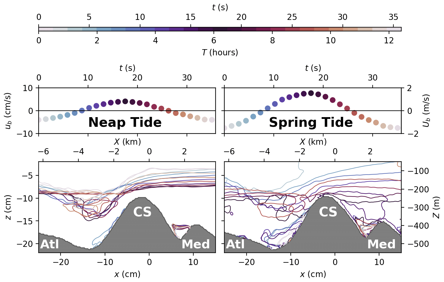
Figure 12 Recirculation and flow detachment at CS. Top row panels display the barotropic velocity u_b above CS for neap tide (left) and spring tide (right) conditions. The bottom panels display the correspondent contours of zero-horizontal velocity u colored as a function of the tidal phase, highlighting the presence of a recirculation area along the west bottom slope of CS during outflow.

Figure 12 presents contours of zero-horizontal velocity $\stackrel{\mathrm{‾}}{u}+\stackrel{\mathrm{̃}}{u}$ colored as a function of the tidal phase, highlighting the presence of a recirculation area along the western bottom slope of CS during outflow in neap tide and spring tide conditions. The tidal phase is expressed in terms of the vertical average of horizontal tidal velocity u_b above CS (top panels). Since the reversal of the tide is not synchronized in both layers, this average gives slightly lower values than expected and previously measured. The detachment is characterized by contours of zero-horizontal velocities at a given phase of the tidal cycle and this is shown in the bottom panels of Fig. 12. During outflow (negative values of u_b), detachment of the Mediterranean layer occurs, generating a reverse flow (eastward) on the western flank of CS. The detachment appears earlier in the tidal phase, persists over a longer time, and has a larger amplitude in spring tide compared to neap tide, consequently delivering stronger bottom turbulence.

According to Prandtl's boundary-layer theory, flow detachment occurs when an adverse pressure gradient is present. We consider a simplified two-dimensional model of the flow, consisting of two immiscible fluid layers separated by a pycnocline at a depth h_p. Detachment occurs when ${\partial }_{x}p>\mathrm{0}$, where x is the along slope coordinate. The total pressure gradient ∂_xp can be decomposed into three components:

$$\begin{array}{}\text{(13)}& {\displaystyle }{\partial }_{x}p={\partial }_x{p}_{\mathrm{b}}+{\mathit{\rho }}_{\mathrm{0}}{g}^{\prime }{\partial }_x{h}_{\mathrm{p}}+{\partial }_x{p}_{\mathrm{nh}},\end{array}$$

where ${\partial }_x{p}_{\mathrm{b}}={\mathit{\rho }}_{\mathrm{0}}g{\partial }_x\mathit{\eta }$ represents the hydrostatic barotropic pressure gradient driven by tidal forcing, ${\mathit{\rho }}_{\mathrm{0}}{g}^{\prime }{\partial }_x{h}_{\mathrm{p}}$ is the hydrostatic baroclinic pressure gradient due to the tilt of the pycnocline h_p, which is always positive for a downslope gravity current, and ∂_xp_nh denotes the non-hydrostatic pressure gradient. Assuming that viscous effects on the tidal flow are negligible, the barotropic pressure gradient can be approximated using Bernoulli's principle:

$$\begin{array}{}\text{(14)}& {\displaystyle }{\partial }_x{p}_{\mathrm{b}}=-{\mathit{\rho }}_{\mathrm{0}}{\partial }_x\left({\displaystyle \frac{u_{\mathrm{b}}^{\mathrm{2}}}{\mathrm{2}}}\right).\end{array}$$

This formulation clearly shows that deceleration of the tidal flow, such as that caused by a bathymetric divergence during outflow, leads to an adverse pressure gradient. Conversely, in regions where the tidal flow accelerates, the barotropic pressure gradient becomes negative, driving the motion of the flow. The sign of the non-hydrostatic pressure gradient cannot be determined from this simplified analysis, although its magnitude can be estimated. Considering L being the typical horizontal length scale, H the vertical length scale, U_g the baroclinic speed scale, U_b the tidal speed scale and g^′ the reduced gravity, the non-dimensional momentum equation in the bottom layer becomes:

$$\begin{array}{}\text{(15)}& {\displaystyle \frac{\mathrm{d}u}{\mathrm{d}t}}={\left({\displaystyle \frac{U_{\mathrm{b}}}{U_{\mathrm{g}}}}\right)}^{\mathrm{2}}{u}_{\mathrm{b}}{\partial }_x{u}_{\mathrm{b}}-{\displaystyle \frac{g^{\prime }H}{U_{\mathrm{g}}^{\mathrm{2}}}}{\partial }_x{h}_{\mathrm{p}}+{\left({\displaystyle \frac{H}{L}}\right)}^{\mathrm{2}}{\partial }_x{p}_{\mathrm{nh}}.\end{array}$$

In our experimental setup, the barotropic pressure gradient is of order one, by design of the tidal forcing. Similarly, the baroclinic pressure gradient scales as the inverse of the squared internal Froude number, which is also of order one. Therefore, the barotropic and baroclinic pressure gradients are expected to be dynamically similar with the real ocean case, as the ratio $U_{\mathrm{b}}/U_{\mathrm{g}}$ and the internal Froude number are preserved by the experimental design. The non-hydrostatic pressure gradient is two orders of magnitude smaller than the hydrostatic terms. Due to the tenfold increase in the aspect ratio in the laboratory compared to oceanic conditions, non-hydrostatic effects are expected to be more pronounced in the experiment. Nevertheless, they only influence the flow characteristics at second order and hence differences can be neglected.

Roustan et al. (2023) inferred strong turbulence near the summit of CS, and observed large overturns on its western flank further downstream during neap tide (compare their Figs. 8 and 11 in transects S2 and S3). These overturns extended down to depths of approximately ≈70 m, significantly larger than those typically produced by shear instabilities, which were estimated to be one order of magnitude smaller. They attributed these large overturns to the detachment of the Mediterranean vein from the western slope of CS during outflow conditions. Their explanation was based on the experiments of Baines (2008), who argued that on the western slope of CS, the gravity-driven flow behaves more like a turbulent plume than a smooth gravity current, resulting in substantial entrainment, rapidly mixing the current with the surrounding water, and causing it to intrude at an intermediate depth rather than to continue following the bottom topography. According to Wesson and Gregg (1994) and Roustan et al. (2024b) high turbulent dissipation rates during neap tide outflows were reported, comparable to those measured under spring tide conditions at the interface between the two layers. They attributed these elevated rates to the Mediterranean intrusion phenomenon proposed by Baines (2008).

Our results clearly indicate that the detachment of the Mediterranean vein is primarily driven by the adverse pressure gradient induced by the barotropic flow, rather than by intense mixing and subsequent intrusion of the Mediterranean vein, a condition present during both spring tide and neap tide phases. This barotropic component of the pressure gradient exceeds the gravitational forcing that drives the dense current downslope, ultimately causing the current to detach from the boundary. Under spring tide conditions, the strength of the barotropic flow leads to reattachment and deceleration of the Mediterranean vein further downstream promoting the transport (advection) of waters mixed through shear instabilities and the internal hydraulic jump further downstream as well. In contrast, during neap tide outflows, it seems that the shear turbulence at the interface, interacts with the boundary-layer turbulence induced by the detachment of the Mediterranean vein, as argued already by Wesson and Gregg (1994), as it can be observed from the TKE distribution and the combined velocity/density fields given in Fig. 4 (but also in Figs. 8 and 10). This effect, combined with a more co-localized positioning of maximum velocity shear and maximum vertical density gradient shown in Fig. 11, results in more localized (less advected) and intense dilution during neap tide conditions as compared to spring tide conditions.

These results therefore suggest the importance of boundary layers (bottom and coastal) in producing TKE and vorticity, which appears to be equivalent to or higher than that produced at the interface between the two layers because of shear. Boundary layers then contribute rather to energy dissipation than to mixing Atlantic and Mediterranean waters in particular during spring tide. These findings may explain why similarly high turbulent dissipation rates levels are observed under both neap tide and spring tide conditions in observational data (Wesson and Gregg, 1994; Roustan et al., 2024b). They also underscore the critical role that topography and bottom boundary layers (friction) play in governing the overall flow dynamics and turbulence and the strong interaction with shear-induced instabilities in promoting water mixing and dilution, an effect that, in some cases, can surpass that of interfacial mixing alone, as already reported in Negretti et al. (2017) and Martin et al. (2019).

4.2.4 Hydraulic criticality

Figure 13 displays the Hovmöller diagrams of the pycnocline depth h_p (${\mathit{\rho }}^{*}=\mathrm{1}/\mathrm{2}$) along the three considered transects (south to north from the top to the bottom panels, see the bathymetry on the left) as a function of the tidal cycle, evolving from maximal outflow to maximal outflow through maximal inflow. The top panels give the variation of the vertically averaged along-strait tidal velocity in both the Atlantic and the Mediterranean for neap tide (left) and spring tide (right) conditions (see the locations indicated in Fig. 1). First of all, an increasing pycnocline depth in the Mediterranean at a given x position moving from the northern to the southern transect can be observed for both neap tide and spring tide conditions, due to the geostrophic slope induced by rotation within the Strait. A remarkable strong variation in time of the pycnocline depth is reported when passing from outflow to inflow (t>8 s) to the east of CS, suggesting that an internal bore is propagating to the East when the flow reverses. This is particularly evident during spring tide conditions in all three transects. The trapped bore is released when the flow criticality is attained. Across-strait variations of the tidal current, stratification conditions, and topography can modulate the shape of the released bore. Lafuente et al. (2015); García-Lafuente et al. (2018) evidenced that the semi-diurnal tidal wave M2 propagates southward in the Strait of Gibraltar. The author exhibited a 15° lag for M2, which corresponds to 29 mn delay between North and South for the external tide. Sanchez-Roman et al. (2018) confirmed that a counter current heading east precedes the tidal signal in the central part of the Strait of Gibraltar. Thus, the tide tilts the internal bore south-eastward, a feature generally preserved in the far field as illustrated by a selection of SAR images presented in Roustan et al. (2024a). Note that differences in the values of phase shifts is attributed to the different considered locations in the different studies (Lafuente et al., 2015; García-Lafuente et al., 2018; Sanchez-Roman et al., 2018; Roustan et al., 2024a) considering that some of them focus on the external tide instead of the internal tide as in our experimental study.

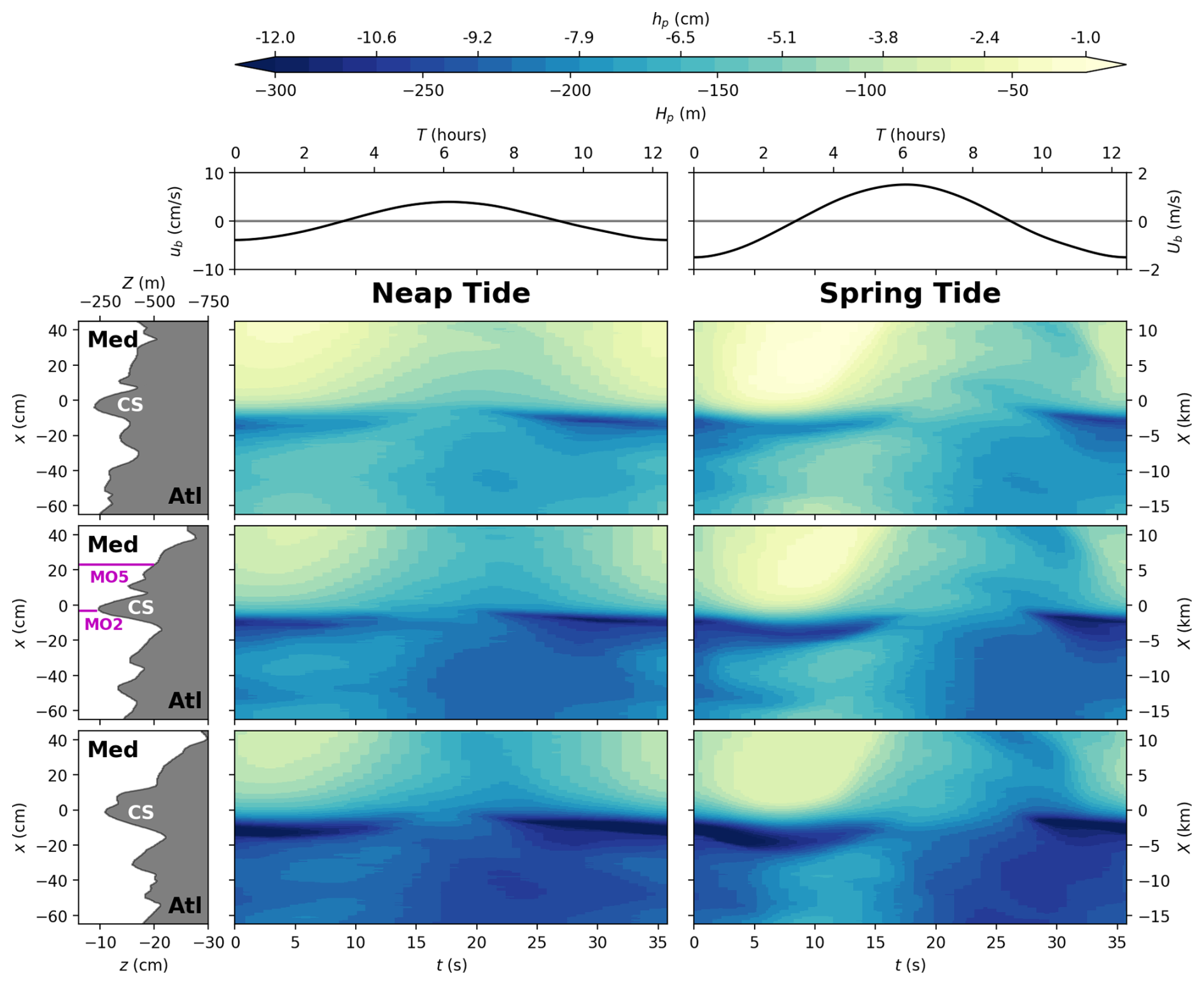
Figure 13 Evolution of the pycnocline depth h_p (${\mathit{\rho }}^{*}=\mathrm{1}/\mathrm{2}$) with the tide from the northern transect (top panels), to the southern transect (bottom panels) in neap tide (left column) and spring tide (right column) conditions. The top panels indicate the vertically averaged along-strait tidal velocity u_b. The bathymetry is given on the left panels. Experimental units (bottom-left), real ocean units (top-right).

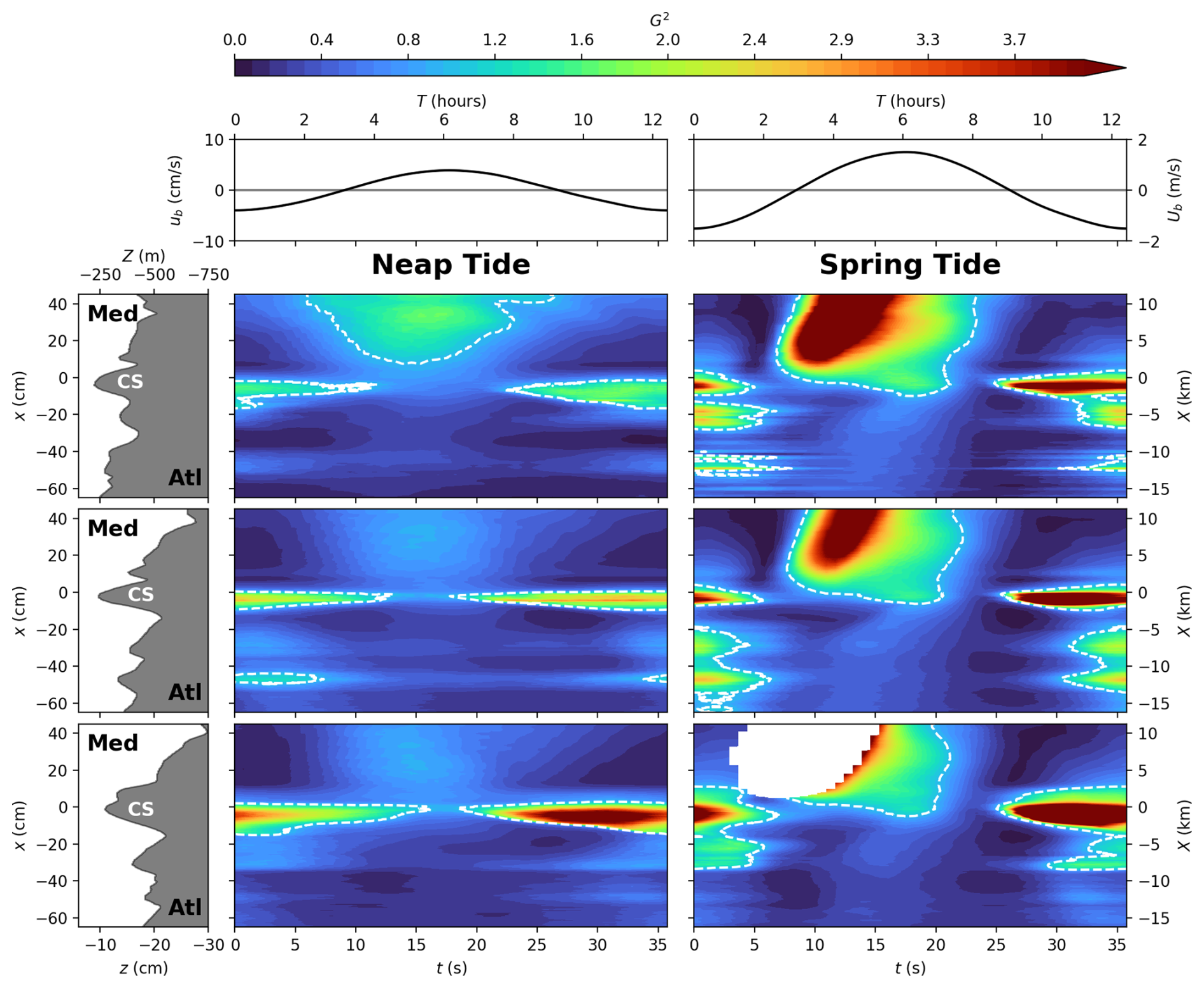
Figure 14 Evolution of the composite Froude number G² (cf. Eq. 10) with the tide for the northern (top panels), the middle (middle panels) and the southern (bottom panels) transects in neap tide (left columns) and spring tide (right column). White dashed lines delimit G²=1. Experimental units (bottom-left), real ocean units (top-right).

We attempted a quantitative estimate of the phase shift using our experimental data; however, it proved difficult to identify and was found to vary from one tidal cycle to another, preventing any robust conclusion. This issue is more appropriately addressed in a forthcoming paper focusing on internal solitary waves (Tassigny et al., 2026).

During outflow (t<10 and t>30 s), we see strong variations in the pycnocline depth around CS, suggesting the presence of hydraulic control for both neap tide and spring tide conditions in all three transects. During inflow, these gradients of h_p are quite reduced, especially for the neap tide conditions, suggesting that the hydraulic control may have been lost at CS in all three transects. Note also the presence of quite high variations in the pycnocline depth in correspondence of the two other topographical features at $x=-\mathrm{30}$ and $x=-\mathrm{45}$ cm, as mentioned in the previous section, for both the neap tide and spring tide conditions.

The composite Froude number of the tidally averaged flow (see Appendix E and Eq. 10) is displayed in the Hovmöller diagram of Fig. 14 for both neap tide and spring tide conditions (left and right panels, respectively). The top panels display the vertically averaged along-strait tidal velocity u_b, whereas the bathymetry is shown on the left panels. The values G²=1 are given by the white dashed lines.

During neap tide conditions, hydraulic criticality is clearly present at CS for ≈88 % of the tidal cycle, and is lost during the maximum amplitude of the inflow $\mathrm{0.38}<t/T_{\mathrm{tide}}<\mathrm{0.5}$. This is consistent with the strong gradients of the pycnocline depth h_p and the strong variations in the averaged vertical velocity $\overline{w}$ reported in Figs. 13 and 4 (and Figs. B1 B2 given in the Appendix B), even though the composite Froude number G² of the mean flow as given in Eq. (10) remains below unity at CS when considering the overall time average. In the southern transect (top panel) an area of G²>1 to the east of CS during inflow appears which may indicate a possible propagation of a bore to the east. Also, as reported previously, we observe locally G²≥1 at $x=-\mathrm{20}\mathrm{cm}$ ($x=-\mathrm{5}\mathrm{km}$ in the real ocean). During spring tide conditions, hydraulic criticality is clearly present at CS for ≈50 % of the tidal cycle, and is lost during inflow. A clear propagation of the bore to the east when control is lost at CS at flow reversal is evident in all three transects under spring tides conditions, which is not evident for neap tide conditions. This difference reflects the different internal solitary waves propagating toward the east that are observed under neap and spring tides, which show to behave differently, an issue examined in the companion paper Tassigny et al. (2026). Further supercritial zones appear during outflow at $x=-\mathrm{30}$ and $x=-\mathrm{45}$ cm (−7.5 and −11.25 km respectively for the real ocean) in correspondence of the other two topographic features during outflow to the west of CS.

As noted above, the frequent misalignment between the pycnocline and the region of maximum shear across tidal phases (cf. Figs. 11, and D1) calls into question the conventional definition of the composite Froude number. Layer depths, h₁ and h₂, can be determined either from the density or the surface of maximum shear of the along-strait velocity, creating inherent ambiguity. Introducing a third layer could mitigate this issue, and a possible definition could delimit the third intermediate layer as the region bounded by the maximum velocity shear and the maximum density gradient, a departure from the more common definition based on intermediate density (Sánchez-Garrido et al., 2011). Different computation methods using different definitions of the interface for both two- and three-layer systems are presented and discussed in detail in the Appendix E, where we conclude that adopting the two-layer method with a local g^′ is the most appropriate definition. For easier comparison with the literature, it is possible to retain the definition of the pycnocline as the intermediate density value (${\mathit{\rho }}^{*}=\mathrm{1}/\mathrm{2}$, approximately equivalent to N_max), although the definition based on S_max as the interface also remains equivalently valid.

The question of the location and permanence of hydraulic controls in the Strait of Gibraltar is central to resolving the long-standing debate on whether the exchange flow is maximal or sub-maximal. If the Strait is bounded by two hydraulic controls, it is hydraulically isolated from both the Mediterranean Sea and the Atlantic Ocean. In that case, the exchange is maximal and does not depend on the pycnocline depth on either side of the Strait, but only on the local bathymetry and the density difference between the two water masses (Armi, 1986; Armi and Farmer, 1986; Lawrence, 1993). The Camarinal and Espartel sills, as well as the Tarifa Narrows, are often cited as likely locations for such controls (Farmer and Armi, 1988). In this paper, we only present measurements at the Camarinal sill section, and the presence of a dual permanent control is thus out of the scope of this paper. However, the speed above Camarinal see have been shown to be constant for almost 25 min (see Fig. 2) despite of changing reservoir conditions, suggesting a maximal exchange regime.

These issues, however, are beyond the scope of the present paper and are therefore not discussed further here. Additional measurements of velocity and density, collected from west of CS to the eastern outer exit of the Strait, as well as over the Espartel and West Espartel sites and including both northern and southern channels, will allow a more comprehensive assessment of these questions and will be addressed in future work.

4.2.5 Transports

Under the Boussinesq approximation, the mean mass transport per unit cross section can be separated into four components. The first corresponds to the advection of the reference density ρ₀ by the mean flow, hereafter referred to as the volume transport. The second arises from the advection of the mean density anomaly, $\mathrm{\Delta }\stackrel{\mathrm{‾}}{\mathit{\rho }}=\mathit{\rho }-{\mathit{\rho }}_{\mathrm{0}}$ by the mean flow, and physically represents the transport of salt. The third and fourth correspond to the transports of the tidal and turbulent flow. Accordingly, the mean transport per unit cross section can be expressed as:

$$\begin{array}{}\text{(16)}& \begin{array}{rl}\underset{h_{\mathrm{b}}}{\overset{\mathrm{0}}{\int }}\stackrel{\mathrm{‾}}{\mathit{\rho }u}\mathrm{d}z& =\underset{\text{volume transport}}{\underbrace{{\mathit{\rho }}_{\mathrm{0}}\underset{h_{\mathrm{b}}}{\overset{\mathrm{0}}{\int }}\stackrel{\mathrm{‾}}{u}\mathrm{d}z}}+\underset{\text{mean buoyancy transport}}{\underbrace{\underset{h_{\mathrm{b}}}{\overset{\mathrm{0}}{\int }}\mathrm{\Delta }\stackrel{\mathrm{‾}}{\mathit{\rho }}\stackrel{\mathrm{‾}}{u}\mathrm{d}z}}\\ & +\underset{\text{tidal transport}}{\underbrace{\underset{h_{\mathrm{b}}}{\overset{\mathrm{0}}{\int }}\stackrel{\mathrm{‾}}{\stackrel{\mathrm{̃}}{\mathit{\rho }}\stackrel{\mathrm{̃}}{u}}\mathrm{d}z}}+\underset{\text{turbulent transport}}{\underbrace{\underset{h_{\mathrm{b}}}{\overset{\mathrm{0}}{\int }}\stackrel{\mathrm{‾}}{{\mathit{\rho }}^{\prime }{u}^{\prime }}\mathrm{d}z}}.\end{array}\end{array}$$

The volume, buoyancy, tidal and turbulent transports are plotted from top to bottom, respectively, of the Fig. 15, for the three transects considered, north to south from left to right. The three tidal forcings are represented by different color's lines, as in the previous Fig. 6. The four terms are arranged from top to bottom according to the amplitude of their contributions to the mean transport, with the volume transport being the dominant component. Each subsequent term is at least one order of magnitude smaller.

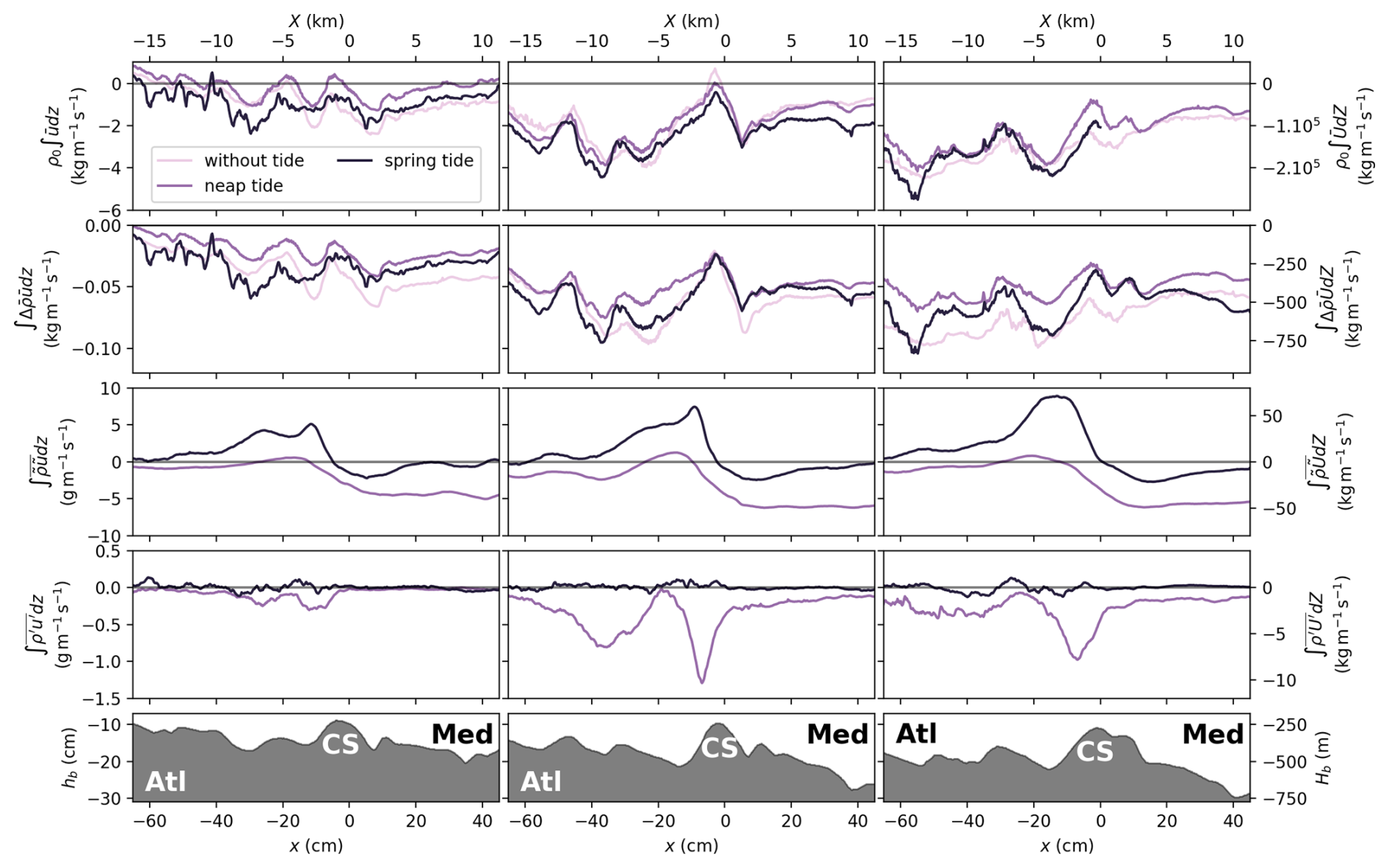
Figure 15 Mean transport contributions (per width unit) for the three transects (from left to right: northern, middle and southern transects), for tidal forcing cases (Without tide, Neap tide an Spring tide). Volume transport (first line), buoyancy transport (second line), tidal transport (third line) and turbulent transport (fourth line).

In an idealized exchange flow without lateral variations, the volume transport (first row panels) should remain zero and constant along the strait axis. In contrast, the results show pronounced local variations at the main topographic constrictions, where strong cross-sectional velocity components develop to bypass the obstacles, as CS and those to the west. Overall, the transport is predominantly negative, indicating that, across the examined transects, a larger volume of Mediterranean water flows westward through CS than Atlantic water eastward. This imbalance is expected to be compensated by an enhanced transport of Atlantic water south of the transects, where the topography features an extended plateau. In addition, the geostrophic slope associated with rotation favors a greater westward transport of Mediterranean water in the northern part of the Strait (see Fig. 3b).

The vertically averaged mean buoyancy transport per unit cross section is displayed in the second row panel of Fig. 15. A significant decrease in transport is observed just upstream of CS for all tidal scenarios, suggesting again the presence of three-dimensional flow structures around the sill, with more water circumventing the sill than overflowing it above the summit. Mass transports are overall everywhere negative and decrease when moving from the southern to the northern transects because of the decreasing depth containing more diluted waters west of CS.

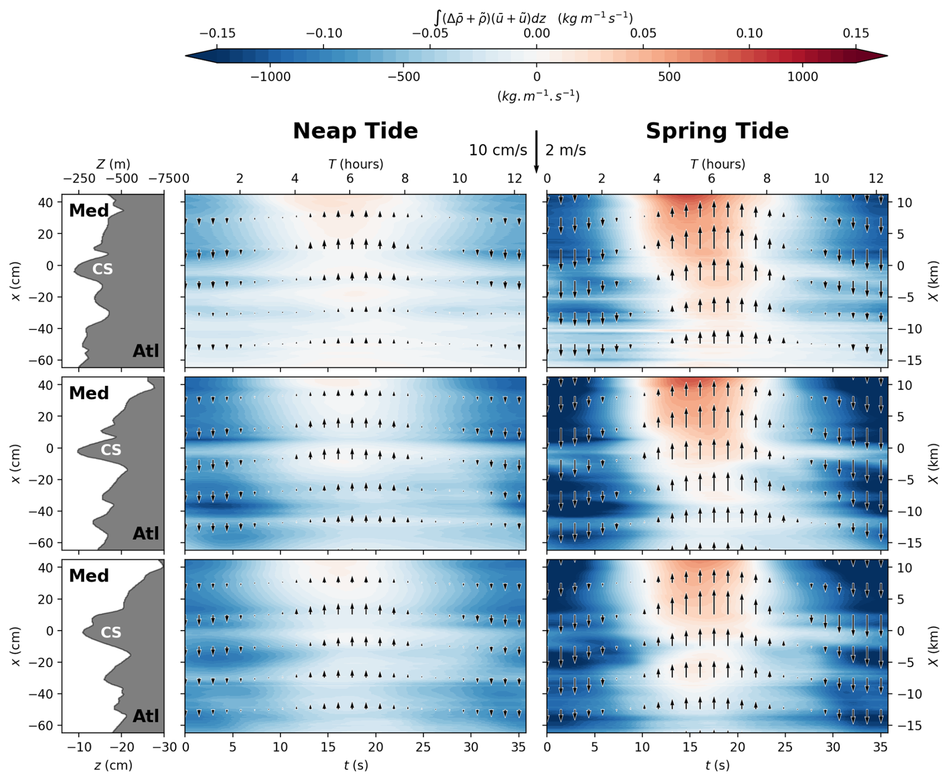
Figure 16 Evolution of the vertically averaged buoyancy transport $\int \left[\mathrm{\Delta }\overline{\mathit{\rho }}+\stackrel{\mathrm{̃}}{\mathit{\rho }}\right](\overline{u}+\stackrel{\mathrm{̃}}{u})\mathrm{d}z$ with the tide for the northern to southern transects from top to bottom panels in neap tide (left columns) and spring tide (right column) conditions. Black arrows are the vertically averaged along-strait tidal velocities u_b, giving the reference of the tidal phase. Experimental units (bottom-left), real ocean units (top-right).

The tidal transport, shown in the next row of panels, exhibits distinct patterns under different tidal forcing conditions. During neap tide, the transport is negative east of the CS and approaches zero immediately west of the sill across all three transects. Under spring tide conditions, by contrast, the tidal transport remains close to zero both east and farther west of the sill, but becomes increasingly positive from north to south in the vicinity of and just west of the sill.

The turbulent transport, presented in the bottom row of Fig. 15, remains near zero for both tidal regimes in the northern transect and for spring tide conditions in the middle and southern transects as well. However, it becomes negative approaching and west of the sill for the neap tide conditions. This negative sign indicates that more diluted waters are advected downstream during neap tide conditions compared with spring tide, for which the transport is dominated instead by the tidal rather than the turbulent component. Figure 16 shows the tidal-mean, vertically averaged buoyancy transport over a full tidal cycle for neap tide (left column) and spring tide (right column) conditions. The volume transport component is not included, as we have shown in the previous Fig. 15 it is two orders of magnitude larger than the buoyancy transport and primarily driven by transverse variability linked to the Strait’s complex topography. buoyancy transport is again enhanced over the southern flanks, where water depth increases. The M2 tidal constituent modulates the mass transport, leading to a pronounced reduction of buoyancy transport during neap tide inflow, and even reversing the direction to positive buoyancy transport during spring tide inflow. Overall, tidal forcing promotes buoyancy transport from the Mediterranean toward the Atlantic.

4.3 Fortnightly modulation of the baroclinic flow

Previous studies (Candela et al., 1989; Helfrich, 1995; García-Lafuente et al., 2002b, a; Vargas, 2004; Vargas et al., 2006; Roustan et al., 2023) reported that the baroclinic flow varies inversely with tidal strength, corresponding to the fortnightly oscillation of the subinertial current induced by the modulation of tidal mixing. According to these authors, the modulation results from enhanced tidal mixing during spring tides, which increases turbulent viscosity and reduces vertical shear between the layers.

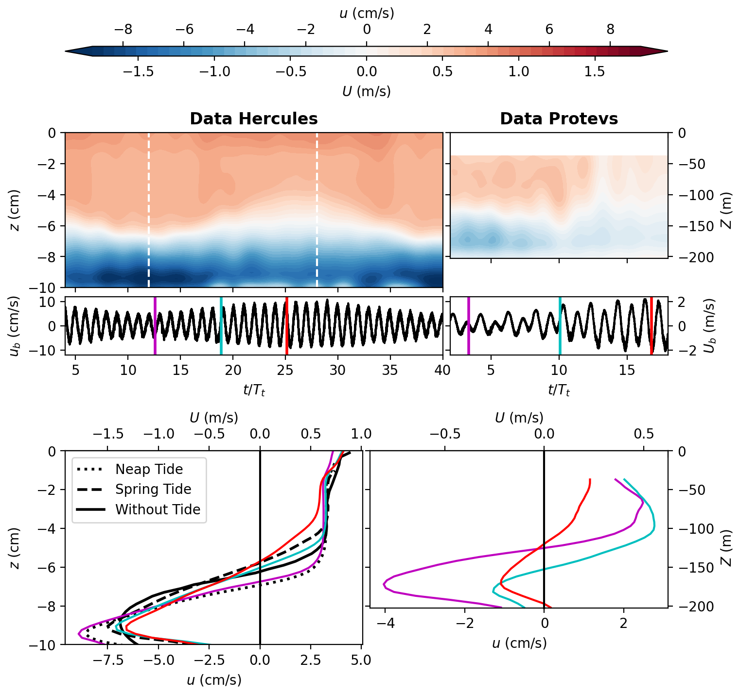
Figure 17 (Top panels) Hovmöller diagram of baroclinic along-strait velocity for the transient tidal forcing experiment (including the M2 and S2 tidal constituents) (left column) and from the PROTEVS GIB20 campaign (Bordois and Dumas, 2020) (right column) at the location of the MO2 mooring. Corresponding barotropic velocities u_b, computed as the vertical average of the along-strait velocity, are given below. (Bottom panels) Vertical profiles of horizontal baroclinic velocity for neap tide (magenta line), spring tide (red line) and intermediate tide (cyan line) in the transient tide experiment. Black lines give the mean profiles of the along-strait velocity for the steady-forcing experiments: without tide – solid lines; neap tide – dotted lines; spring tide – dashed lines.

Using velocity data obtained from the experiment with transient tidal forcing (including the M2 and S2 tidal constituents) to allow direct comparison with observational data, we observe a similar reduction in baroclinic flow to that reported by previous authors when considering the same location (MO2 mooring at the CS summit) and applying identical data filtering. This behavior is illustrated in Fig. 17.

The top panels display the along-strait velocity component, computed from the velocity data using an eighth-order Butterworth low-pass filter with a cutoff period of 95 s (35 h), thereby retaining long-term and subinertial components following the approach of Roustan et al. (2023) based on the methodology of Vargas et al. (2006). It shows the temporal evolution of the filtered along-strait velocity throughout the analyzed interval and demonstrates excellent agreement between the transient tide experiment (left column) and with the PROTEVS GIB20 measurements (Bordois and Dumas, 2020) (right column). The ∼30 % reduction in net baroclinic horizontal flow with increasing tidal forcing from neap tide to spring tide is also consistent with earlier field measurements and modeling studies (Candela et al., 1989; Helfrich, 1995; García-Lafuente et al., 2002b, a; Vargas, 2004; Vargas et al., 2006; Roustan et al., 2023).

The second row panels presents the time series of the barotropic flow, marking three instants in the tidal cycle corresponding to neap tide amplitude (magenta line), spring tide amplitude (red line) and intermediate amplitude (cyan line).

In the third row, we compare the tidally averaged steady-forcing experiments (without tide, solid lines; neap tide, dotted lines; spring tide, dashed lines) with the results of the transient-forcing experiment (colored lines) at three different time instants corresponding to the above mentioned varying tidal strengths. For the purely baroclinic case (solid black line), the lowest maximum along-strait baroclinic velocities are found in the Mediterranean layer. When a constant tidal forcing is applied, the maximum along-strait baroclinic velocity decreases inversely with tidal strength. Similarly, in the transient-forcing experiment, the maximum along-strait baroclinic velocity also decreases with increasing tidal amplitude in agreement with the in situ observations of the aforementioned authors (although the reduction is slightly weaker than in the steady-forcing cases in the experiments).

Horizontal maximum along-strait baroclinic velocities decrease from approximately 9.5 to about 6.5 cm s⁻¹, corresponding to a ≈ 30 % reduction from neap tide to spring tide tidal forcing. Moreover, the shape of vertical profiles of along-strait velocity changes systematically with the imposed tidal strength.

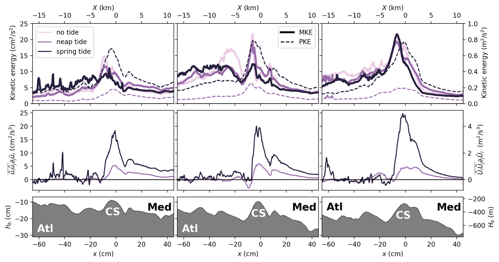
Figure 18 Kinetic energy characteristics at CS for the three tidal conditions the three transect from north, to south (from left to right). First row panels display the vertically averaged mean kinetic energy (MKE, thick lines) and the vertically averaged tidal kinetic energy (PKE, dashed lines). The second row panels display the transfer rate between mean kinetic energy and tidal kinetic energy. Positives values indicate energy transfer from the tidal to the mean flow.

Different mechanisms could explain the reduction of net baroclinic flow with increasing tidal amplitude at the considered location.

The first, proposed by earlier authors, attributes it to enhanced mixing during spring tide. However, we have shown earlier in this paper that mixing is, in fact, stronger during neap tide, making this explanation unlikely.

A second possible mechanism is the transfer of periodic (tidal) kinetic energy into the mean kinetic energy of the flow. These quantities, along with the turbulent kinetic energy (TKE), are shown in the top panels of Fig. 18 for the three analyzed transects (north, middle, and south, from left to right). The different colored lines indicate the increasing strength of the tidal flow, with darker colors representing stronger tides. In the northern and middle transects, the mean kinetic energy at the CS clearly decreases as tidal strength increases, whereas the opposite trend is observed in the southern transect. Moreover, outside the sill summit, these tendencies exhibit strong spatial variability in both the transverse and longitudinal directions.

The bottom panels of Fig. 18 show the conversion rate between periodic kinetic energy and mean kinetic energy, given by $\stackrel{\mathrm{‾}}{\stackrel{\mathrm{̃}}{u}\stackrel{\mathrm{̃}}{w}}({\partial }_z\stackrel{\mathrm{‾}}{u}+{\partial }_x\stackrel{\mathrm{‾}}{w})+\stackrel{\mathrm{‾}}{{\stackrel{\mathrm{̃}}{u}}^{\mathrm{2}}}{\partial }_x\stackrel{\mathrm{‾}}{u}+\stackrel{\mathrm{‾}}{{\stackrel{\mathrm{̃}}{w}}^{\mathrm{2}}}{\partial }_z\stackrel{\mathrm{‾}}{w}$ in [W kg⁻¹]. For tidal flow extracting energy from the mean flow (i.e., decelerating it), this conversion term should be negative. However, the figure shows it is positive everywhere, especially around the sill, indicating that the tidal flow transfers energy to the mean flow, thereby accelerating it. This trend intensifies with tidal forcing: the curve corresponding to spring tide conditions (black line) exceeds that for neap tide (purple line) near the sill. Consequently, the observed decrease in net along-strait baroclinic velocity at the sill cannot be attributed to the tidal-to-mean energy transfer.

Another possible mechanism which may explain the reduced net baroclinic velocity when tidal amplitude increases is the phenomenon of the tidally driven eddy fluxes, which can account for large portions (up to 40 %–60 %) of the total exchange transport (Bryden et al., 1994; Vargas et al., 2006) in regions where hydraulic control is intermittently lost, such as at Camarinal. These studies (see also García-Lafuente et al., 2002a; Morozov et al., 2002) state that an increase in tidal amplitude leads to a decrease in the net buoyancy transport, which is instead compensated by tidal transport via the eddy fluxes. Tsimplis and Bryden (2000); Bryden et al. (1994) documented strong tidal variability and interface depth oscillations at CS, which are associated with significant fortnightly and monthly fluctuations in layer transports that reflect the influence of tidal eddying on exchange dynamics. These eddy fluxes, arising from the positive correlation between vertical interface and tidal current fluctuations, contribute to augment the net transport beyond what is predicted by traditional, steady two-layer hydraulic theory.

In the present study, we interpret the concept of eddy fluxes as representing the tidal and turbulent transports defined in Eq. (16) and shown in Fig. 15 (third and fourth rows, respectively). As discussed above with Fig. 15, the tidal and turbulent transports are approximately one order of magnitude smaller than the volume and buoyancy transports. In particular, the tidal transport is of order $\approx \mathrm{5}\times {\mathrm{10}}^{-\mathrm{3}}$ kg m⁻³ (the turbulent transport is even smaller), whereas the buoyancy transport is of order $\approx \mathrm{5}\times {\mathrm{10}}^{-\mathrm{2}}$ kg m⁻³. Although we observe an increase in tidal transport with increasing tidal strength (cf. third row of Fig. 15), this increase is not sufficient to explain the corresponding reduction in buoyancy transport. Therefore, the diminished net baroclinic velocity with increasing tidal amplitude reported in our experiments, as well as in observational data, cannot be attributed to the action of eddy fluxes alone.

The last possible mechanism is the cross-strait spatial variability. The analysis along and between transects reveals pronounced variability in both the longitudinal and transverse directions, underscoring the strongly three-dimensional nature of the flow. When the tidal forcing is strong, the flow bypassing the obstacle laterally increases compared to what overflows it. This conclusion is consistent with the computed transports shown in Fig. 15, which display increasingly large transport values as the tidal forcing decreases at the CS summit, while also exhibiting pronounced spatial variability in both the longitudinal and transverse directions.

Therefore, from these considerations we conclude that fluxes and transports cannot be accurately derived from horizontally or vertically averaged fields. The significant spatial heterogeneity makes full three-dimensional budgets indispensable for correctly quantifying these exchanges and for drawing robust physical conclusions.

5 Conclusions and perspectives

In this study, we present the design and implementation of a large-scale physical model representing the Strait of Gibraltar and its surrounding regions. The selection of this key area in ocean dynamics is justified by its intense, small-scale, non-hydrostatic processes, which have significant feedback effects on larger-scale circulation patterns in both the Mediterranean Sea and the North Atlantic Ocean.

The novelty of this work lies in the unprecedented level of realism achieved in a laboratory setting. The model incorporates the realistic topography of a 250 km × 150 km area, maintains a limited horizontal-to-vertical stretching ratio of 10, and includes both barotropic and baroclinic forcing as well as the Coriolis effect due to Earth's rotation. Utilizing advanced measurement techniques, we captured essential flow characteristics, including velocity and density fields, which confirmed the dynamic similarity of our model to oceanic observations (Roustan et al., 2023; Gasser et al., 2017).

Through combined velocity and density measurements across vertical transects in the Strait and near the critical region of Camarinal Sill (CS), we reveal the dominant role of bottom boundary layers. These generate significantly higher levels of turbulent kinetic energy compared to the sheared interface between Mediterranean and Atlantic waters. We attribute the enhanced impact of bottom boundary layers to the detachment of the gravity current from the sloping topography west of CS, induced by an adverse pressure gradient during outflow, when superimposed with tidal flow. This provides a new explanation for the previously debated detachment of the Mediterranean vein observed via moorings on the western side of CS (Baines, 2008; Roustan et al., 2024b), attributing it to boundary layer separation rather than due to the gravity current intrusion after enhanced interfacial mixing produced by shear instabilities or the internal hydraulic jump as proposed by previous authors.

The detachment becomes even more pronounced during spring tides, leading to advection of the diluted waters further westward beyond CS. In contrast, during neap tides, the turbulent kinetic energy from bottom boundary layers coincides with the turbulent kinetic energy at the interface between the two layers. This dual mechanism may explain the high dissipation rates observed in-situ during neap tides (Wesson and Gregg, 1994; Roustan et al., 2024b), an issue which is investigated in detail in a forthcoming paper (Tassigny et al., 2026b). Overall, we observe up to 20 % reduction in density west of CS when tidal forcing is active, compared to purely baroclinic conditions, underscoring the crucial role of tidal dynamics in promoting full-depth mixing, as opposed to solely stratified shear-induced interfacial mixing.

We also evaluated the composite internal Froude number, using temporally averaged velocity and density data under the assumption of a two-dimensional, two-layer flow. Results from the overall time averaged analysis reveal that relying solely on the criteria G²=1 is insufficient to identify internal hydraulic criticality. Instead, critical conditions are better indicated when additionally abrupt changes in vertical velocity, sharp pycnocline plunges, and local thickening of the mixed layer coincides. When averaged over the tidal cycle, instead, values of G²⩾1 are consistently found at CS during outflow for both neap tide and spring tide conditions across all three considered transects. However, during spring tide, hydraulic control is lost for 50 % of the tidal cycle during inflow and this loss of control propagates eastward as an internal bore. Additional regions of G²⩾1 are identified west of CS, associated with strong pycnocline gradients and vertical velocity changes, suggesting multiple sites of hydraulic control out of CS during spring tide. For neap tide conditions control is lost only for 12 % of the tidal cycle during inflow and only one further location present a clear control west of CS.

The observed propagation of hydraulic control, together with sudden pycnocline displacement during tidal reversals, suggests the release of a trapped internal bore moving eastward. The volume and mean buoyancy transports are up to two orders of magnitude larger than the tidal and turbulent transports and primarily driven by transverse variability linked to the Strait’s complex topography. Fortnightly variations of the baroclinic velocity of the order of 20 %–30 % are shown to be primarily linked to the complex 3D dynamics. Mass transport is found to be positive across all transects and tidal phases, indicating a net flux into the Atlantic Ocean. Also, tidal forcing produces a marked shift between the maximum velocity shear and vertical density gradients, with possible implications for turbulent mixing parametrizations and proper definition of the interface, for example for the composite Froude number.

These findings highlight the invaluable role of laboratory experiments in advancing our understanding of oceanic physical processes. In particular, we demonstrate that experimental modeling at a high level of realism leads to a coverage of the dynamics which is comparable to numerical experiments even in realistic configurations. It becomes a powerful and efficient approach not only to complement numerical modeling but also to bridge the gap between experimental, observational, and numerical methodologies.

The HERCULES experimental campaign comprises approximately 140 experiments, resulting in an extensive dataset that addresses a wide range of regions and physical processes. These experiments include configurations with purely barotropic and purely baroclinic forcing, which are particularly valuable for the calibration and validation of numerical models. Given the already substantial length of the present manuscript, it was obviously not possible to include results from all investigated areas and processes.

In addition to the overall dynamics in the Strait presented here, a dedicated set of experiments focuses on the generation and propagation of internal solitary waves in the Alboran Sea. These experiments allow for the investigation of different generation mechanisms and of the various wave types produced under increasing tidal strength; the corresponding results are presented in the companion paper by Tassigny et al. (2026). The free surface wind effects (blowing constantly toward the East) on internal solitary waves dynamics has been addressed with combined PIV and interface measurements for different amplitudes of the wind speed and the tide. High-frequency analyses in the Strait, including turbulence characteristics and fluxes as well as entrainment and mixing budgets in the region of CS, also valuable to correctly parametrize turbulence in numerical models, are the subject of two additional publications currently in preparation (Tassigny et al., 2026c, b).

Further dedicated experiments address transient dynamics, including the S2 tidal constituent, and reveal preliminary yet intriguing results related to hysteresis and memory effects in the flow. Synoptic measurements of high-frequency density and velocity were also conducted along southern and northern transects of the Espartell sill, extending down to the West Espartell site, delivering a unique dataset to estimate turbulent fluxes and mixing characteristics (Tassigny et al., 2026a). Another subset of experiments focuses on measurements in the Gulf of Cadiz, tracking the propagation of the Mediterranean Outflow and the associated large-scale Atlantic circulation. These experiments provide insight into the synoptic coupling between the Strait and the Gulf of Cadiz, and their results are presented in an additional companion paper (Bardoel et al., 2026). Complementary measurements were conducted in both the Gulf of Cadiz and the Strait using an enhanced density contrast between the Atlantic and Mediterranean basins. These experiments enable the investigation of potential climate-driven variations in the density of the Mediterranean Outflow and their subsequent impact on its downstream evolution in the Gulf of Cadiz.

We encourage interested members of the community to contact us regarding access to and use of the HERCULES experiment dataset.

Appendix A: Planar Laser Induced Fluorescence (PLIF) calibration procedure

In stratified flow experiments, accurately matching the refractive indices of the heavy and light fluids is essential for precise optical flow diagnostics. This is commonly achieved by using a saltwater solution as the denser fluid and an ethanol-water mixture as the lighter one. However, Daviero et al. (2001) showed that variations in refractive index can often be neglected if the salt and dye concentrations remain below specific limits: density differences under 20  kg m⁻³ and dye concentrations (c₀) below 70 µg L⁻¹. These conditions are satisfied in the present study, with c₀=5 µg L⁻¹, ensuring minimal optical distortion and reliable diagnostic results.

The Laser Induced Fluorescence (LIF) technique was employed to determine the density distribution across three vertical planes in the Strait of Gibraltar, coinciding with the Particle Image Velocimetry (PIV) measurement planes. Rhodamine 6G was introduced into the saline Mediterranean water at the onset of the experiment. This fluorescent dye exhibits an absorption maximum near 530 nm and an emission maximum around 550 nm. Upon illumination with a laser operating at 532 nm, the dye emits fluorescence, the intensity of which is proportional to the local Rhodamine concentration. To account for the attenuation of laser light as it propagates through the fluid, corrections based on the Beer–Lambert law are applied. Accordingly, for a pixel representing a fluid volume located at position (x,z), with I₀ denoting the incident laser intensity, c the Rhodamine concentration, which is indepedent of the pixel's position for the calibration procedure, and E the intensity of the emitted fluorescence recorded by the camera, the following relationship applies:

$$\begin{array}{}\text{(A1)}& {\displaystyle }E(x,z)=c\mathit{\alpha }{I}_{\mathrm{0}}{e}^{-(a_{\mathrm{w}}+\mathit{ϵ}c)z}+\mathit{\beta }\end{array}$$

with a_w the absorption coefficient of water, ϵ the absorption coefficient of Rhodamine and α, β adjustable constants (here we discard the absortion coefficient of salt and ethanol which can be neglected as suggested by Negretti et al., 2022).

To determine the values of β and αI₀, an in-situ calibration procedure was conducted. This involved capturing fluorescence images for six known Rhodamine concentrations. The calibration coefficients were then estimated through linear regression. It was assumed that the laser illumination at the free surface, I₀, is uniform across the measurement plane, and that each pixel of the camera sensor exhibits identical sensitivity to light. The latter assumption is justified by the fact that the image edges – where sensor sensitivity may vary – were cropped. Consequently, the parameters I₀, α and β are considered spatially invariant with respect to the (x,y) coordinates. As values for very low concentration are highly subject to noise, the linear regression is weighted by the coefficient of determination of the last linear regression (colorbar in Fig. A1a). We measured $a_{\mathrm{w}}=\mathrm{3.2}\times {\mathrm{10}}^{-\mathrm{3}}$ cm⁻¹ and $\mathit{ϵ}=\mathrm{3.7}\times {\mathrm{10}}^{-\mathrm{3}}$ cm⁻¹ µg L⁻¹, which values are very close to values measured by Negretti et al. (2022). For each known Rhodamine concentration, a linear regression of the measured fluorescence intensity E on the camera sensor is performed independently at each pixel of the image. This procedure yields estimates of the calibration constant β and the combined proportionality term $c\mathit{\alpha }{I}_{\mathrm{0}}{e}^{-(a_{\mathrm{w}}+\mathit{ϵ}c)z}$, which varies with depth z. To extract the attenuation coefficient (a_w+ϵc), a second linear regression is conducted on the logarithm of the proportionality term obtained from the initial fit.

The resulting attenuation coefficients, calculated across all horizontal rows of pixels and for each of the six Rhodamine concentrations, are shown in Fig. A1a. These values are subsequently fitted using a linear regression to determine the individual absorption coefficients a_w (for water) and ϵ (for Rhodamine). Since measurements at very low dye concentrations are more susceptible to noise, the regression is weighted by the coefficient of determination from the preceding logarithmic fit, as indicated by the colorbar in Fig. A1a. The calibration yielded absorption coefficients of $a_{\mathrm{w}}=\mathrm{3.2}\times {\mathrm{10}}^{-\mathrm{3}}$ cm and $\mathit{ϵ}=\mathrm{3.7}\times {\mathrm{10}}^{-\mathrm{4}}$ cm⁻¹ µg l⁻¹, which are in close agreement with the values reported by Negretti et al. (2022). Figure A1b plots the light on the sensor E against the corrected concentration of Rhodamine ce${}^{-(a_{\mathrm{w}}+\mathit{ϵ}c)z}$ for each pixel of the image. A final linear regression is performed to compute the value of αI₀ and β. Knowing all the parameters, the concentration of Rhodamine can thus be recovered using the formula:

$$\begin{array}{}\text{(A2)}& {\displaystyle }c\left(z\right)={\displaystyle \frac{\left[E\left(z\right)-\mathit{\beta }\right]\frac{e^{a_{\mathrm{w}}z}}{\mathit{\alpha }}}{\mathrm{1}-\mathit{ϵ}{\int }_{\mathrm{0}}^z\left[E\left(z\right)-\mathit{\beta }\right]\frac{e^{a_{\mathrm{w}}z}}{\mathit{\alpha }}\mathrm{d}z}}.\end{array}$$

Retrieving the concentration of calibration images from this formula, an error below 5 % is found. Following a detailed analysis of the data, an additional correction was applied to account for the absorption of fluorescent light emitted by Rhodamine along its path to the camera. Figure A1c displays five representative density profiles: four located east of CS at $x=-\mathrm{45.2}$, −35.2, −25.2 and −15.2 cm all corresponding to the outflow phase. In this figure, dashed lines represent uncorrected profiles, dotted lines correspond to profiles corrected for absorption along the vertical laser path, and solid lines show profiles corrected for both in-plane absorption and attenuation along the path to the camera. During the experiment, the imposed density contrast between Mediterranean and Atlantic waters was Δρ=19 kg m⁻³. By applying both absorption corrections, the density profiles East of CS reveal a well-defined, uniform lower layer, with the density difference between the upper and lower layers closely matching the experimental conditions, as shown in Fig. A1c by the vertical solid line. The correction of the absorption is also significant west of CS: although the absence of correction does not result in an apparently unstable profile, neglecting it would lead to an overestimation of the mixing intensity.

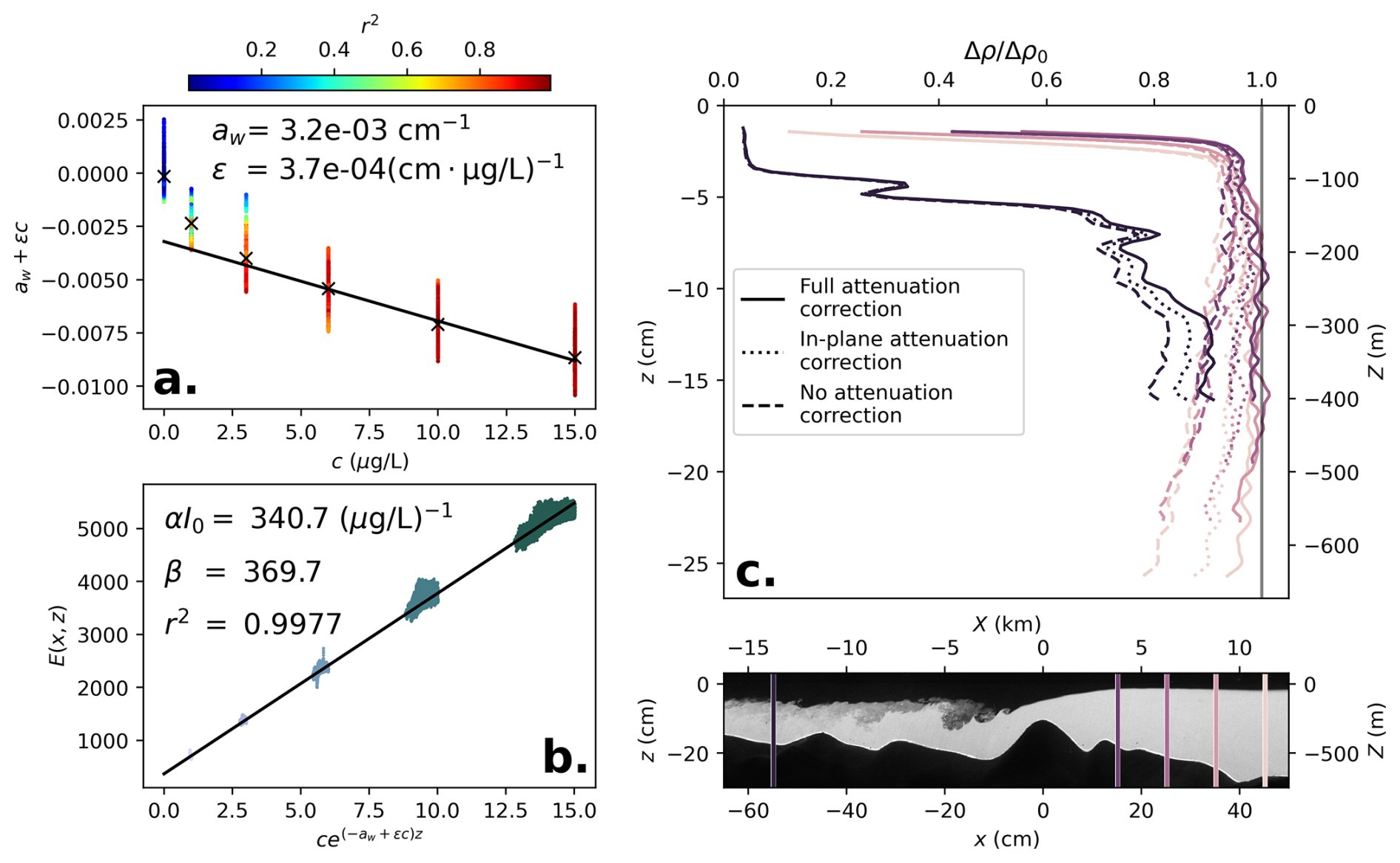
Figure A1 (a) Attenuation coefficient as a function of Rhodamine concentration. The colorbar indicates the determined coefficient r² of each linear regression used to compute the attenuation coefficient. (b) Light E on the camera sensor against the corrected Rhodamine concentration ce${}^{-(a_{\mathrm{w}}+\mathit{ϵ}c)z}$. Black lines represent linear interpolations. (c) Effect of the LIF corrections on five vertical density profiles during outflow. Dashed lines represent no correction, dotted lines include correction for absorption along the laser paths, solid lines include additionally the absorption of light along the path to the camera. The vertical solid line indicates the initial imposed density difference between Mediterranean and Atlantic waters for reference.

Appendix B: Time averaged characteristics in the northern and southern transects at CS in the Strait

Figures B1 and B2 show the velocity and density fields around the Camarinal Sill, averaged over seven tidal cycles during the stationary maximal exchange regime for the northern and southern transects, respectively, under three tidal forcing scenarios: weak tides (without tide, left column), neap tides (neap tide, middle column), and spring tides (spring tide, right column). In the top panels, arrows indicate the in-plane velocity vectors, while the colormap represents the dimensionless density ratio ρ^*. Along-strait (u) and vertical (w) velocity components are displayed in the second and third rows, together with iso-density contours shown as black and grey lines. The time-averaged composite Froude number, G², is indicated by the purple line, and the bottom panels display the turbulent kinetic energy (TKE).

The main features observed, namely, density dilution enhanced in neap tide conditions, vertical displacement between maximum density and along-strait velocity gradients, boundary layer detachment of the Mediterranean flow on the western flank of CS, and elevated turbulent kinetic energy near the bottom topography relative to the sheared interface, are consistent across the northern and southern transects and with the results presented in Sect. 4.1 in the middle transect.

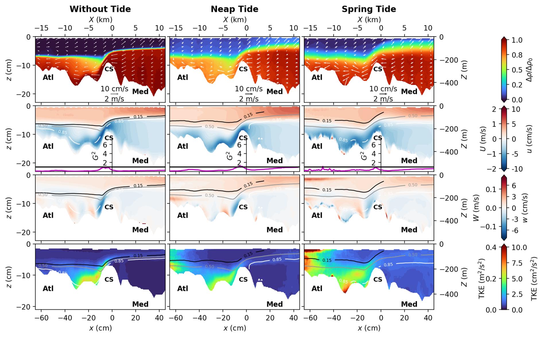
Figure B1 Mean flow characteristics for the northern transect passing north of the CS summit (cf. Fig. 3b), for the three tidal forcings: without tide, neap tide, and spring tide from left to right. The x axis represents the along-transect coordinate, being positive toward the east. The first row displays the mean density with the averaged velocities $(\stackrel{\mathrm{‾}}{u},\stackrel{\mathrm{‾}}{w})$ (white arrows). The second and third rows panels display the mean horizontal u and vertical w velocities, respectively, superposed with the $\mathrm{\Delta }\mathit{\rho }/\mathrm{\Delta }{\mathit{\rho }}_{\mathrm{0}}=$ 0.15, 0.5, and 0.85 (black, grey, and white lines respectively). In between, the composite Froude number G² is displayed as a purple line. The last row panels display the turbulent kinetic energy $\mathrm{TKE}=(\stackrel{\mathrm{‾}}{u^{\prime \mathrm{2}}}+\stackrel{\mathrm{‾}}{w^{\prime \mathrm{2}}})/\mathrm{2}$. Experimental units (bottom-left), real ocean units (top-right).

Figure B2 Same as Fig. B1 but for the southern transect.

Appendix C: Dilution

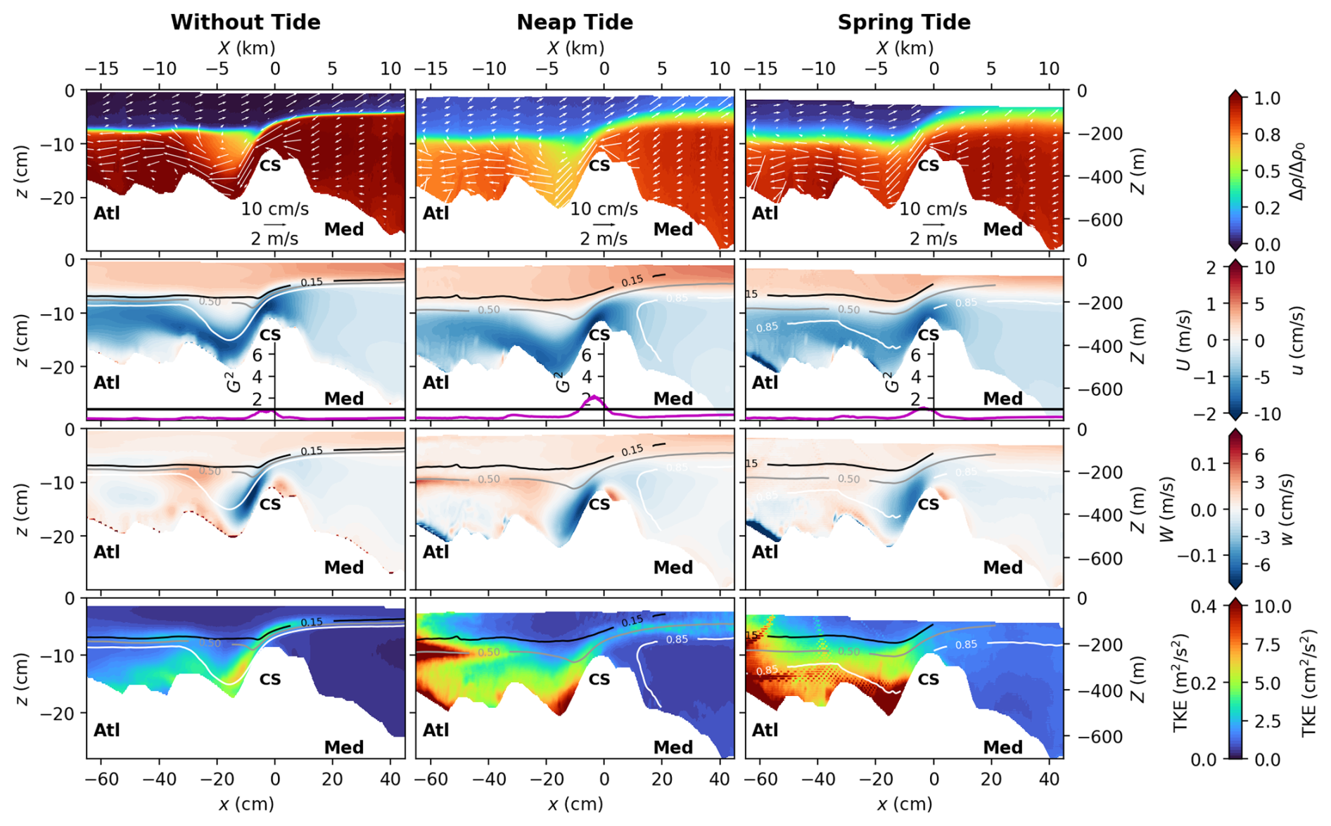
Figure C1 shows the mean dimensionless density difference ratio, ${\mathit{\rho }}^{*}\equiv \mathrm{\Delta }\mathit{\rho }/\mathrm{\Delta }{\mathit{\rho }}_{\mathrm{0}}$, at five locations along the central transect for the no-tide (left column), neap-tide (center column), and spring-tide (right column) cases. The two easternmost locations correspond to the MO2 and MO5 moorings of the PROTEVS campaign. In all cases, the mean reduced density in the bottom layer decreases westward. Dilution is strongest during neap tide, with the mean bottom-layer density west of CS decreasing by approximately 20 % relative to that at MO5. This dilution is significantly reduced during spring tide, with a density decrease of only a few percent across CS. The baroclinic case differs slightly from the two tidal cases, exhibiting the formation of a third mixed layer west of the sill with ${\mathit{\rho }}^{*}\simeq \mathrm{0.8}$, while the bottom-layer dilution remains limited to only a few percent.

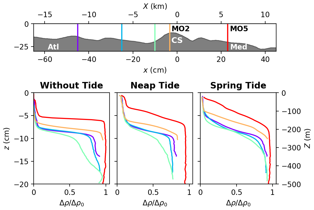
Figure C1 Mean dimensionless density-difference ratio, ${\mathit{\rho }}^{*}\equiv \mathrm{\Delta }\mathit{\rho }/\mathrm{\Delta }{\mathit{\rho }}_{\mathrm{0}}$, at five locations along the central transect for the no-tide (left column), neap-tide (center column), and spring-tide (right column) cases. The two easternmost locations correspond to the MO2 and MO5 moorings of the PROTEVS campaign.

Appendix D: Vertical profiles of density and along-strait velocity gradients east and west of the CS summit

In this section we present additional evidence of the shift between the maximum vertical gradient of along-strait velocity and density. Figure D1 displays correlation maps between the vertical velocity shear S (see Eq. 11) (green colormap) and the Brunt–Väisälä frequency N (colored iso-contours) for maximum outflow, high water slack, maximum inflow and low water slack (from top to bottom, see bottom panel for tidal reference). Neap tide conditions are shown in the left panels and spring tide conditions in the right panels. The figure demonstrates that a frequent shift between the locations of maximum S and N west of CS and up to 20 cm (5 km in the real ocean), a phenomenon that can have implications for parameterizing turbulent exchange and for the definition of the composite internal Froude number for reliable diagnostics of hydraulic control.

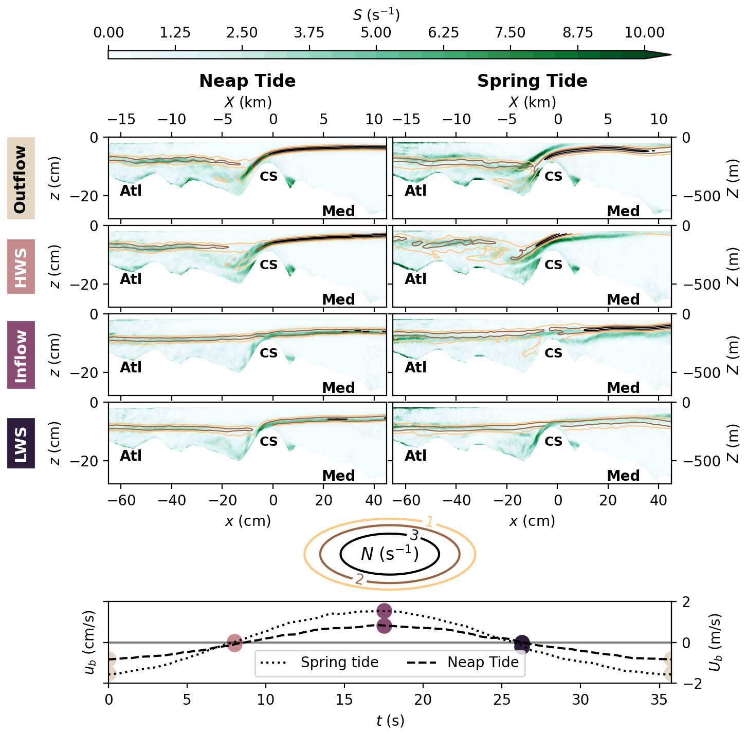
Figure D1 Correlation maps between the vertical velocity shear S (see Eq. 11) (green colormap) and the Brunt–Väisälä frequency N (colored iso-contours) for maximum outflow, high water slack, maximum inflow and low water slack (from top to bottom, see bottom panel for tidal reference). Neap tide (left panels) and spring tide (right panels). Experimental units (bottom-left), real ocean units (top-right).

Appendix E: Computing the composite Froude number

The local composite Froude number G² provides an indication of the local criticality of the flow. It is defined by assuming a two-layer exchange flow with mean layer thicknesses ${\overline{h}}_i$ and constant mean horizontal velocities ${\overline{u}}_i$:

$$G^{\mathrm{2}}={\displaystyle \frac{{\overline{u}}_{\mathrm{1}}^{\mathrm{2}}}{g^{\prime },{\overline{h}}_{\mathrm{1}}}}+{\displaystyle \frac{{\overline{u}}_{\mathrm{2}}^{\mathrm{2}}}{g^{\prime },{\overline{h}}_{\mathrm{2}}}},$$

where g^′ is the reduced gravity. Mathematically, the condition G²≥1 is necessary for the development of a stationary shock such as an internal hydraulic jump (Armi and Farmer, 1985; Sannino et al., 2007). However, this condition alone does not guarantee hydraulic control at the scale of the entire strait section (Pratt, 2008). To compute G², several authors discuss the possibility of using a two-dimensional, two-layer model, although the validity of this assumption remains a matter of debate.

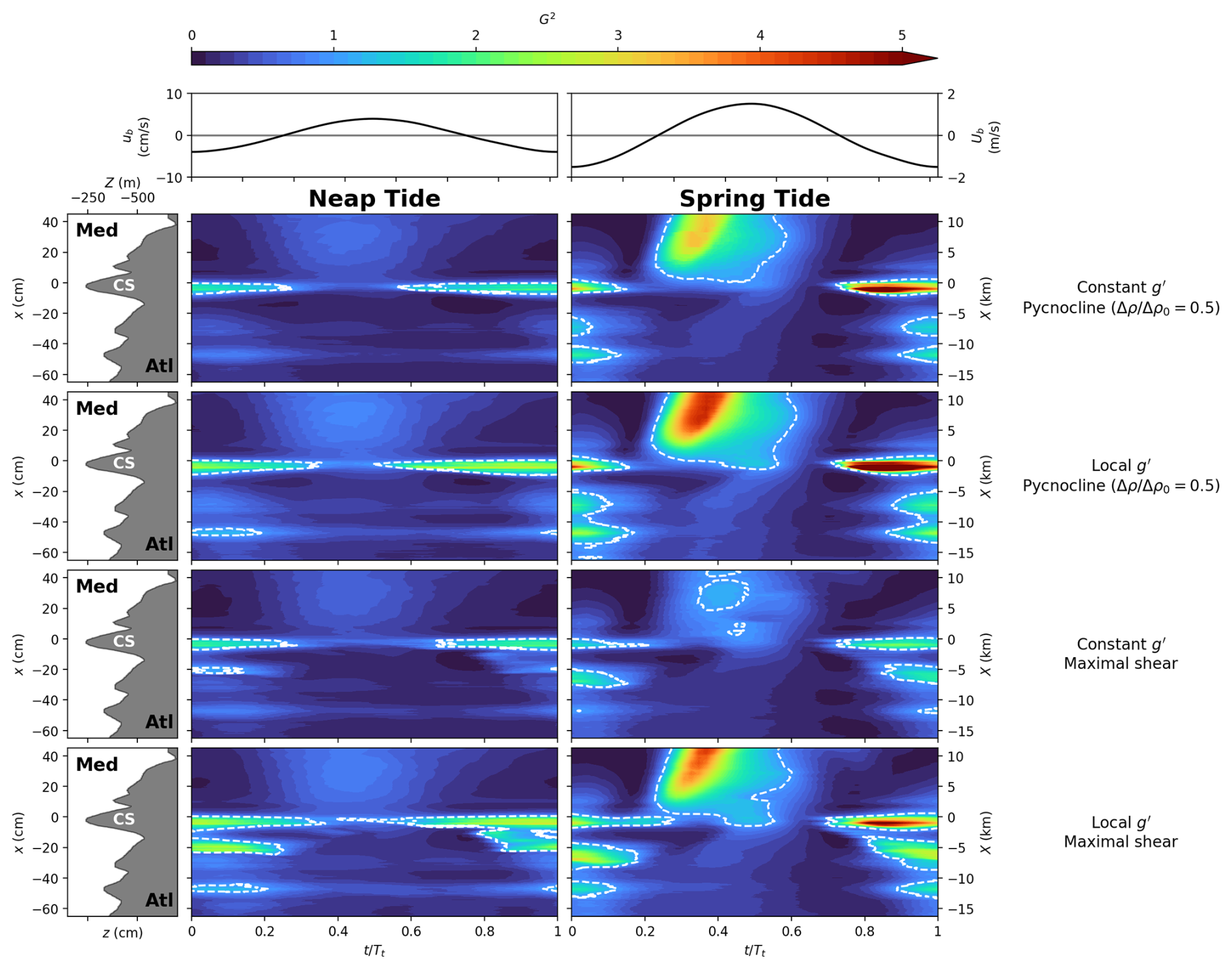
Figure E1 Comparison between different methods for calculating the composite Froude number G² for neap tides (left panels) and spring tides (right panels). The first row shows the method considering a constant reduced gravity g^′ and a pycnocline defined by $\mathrm{\Delta }\mathit{\rho }=\mathrm{\Delta }{\mathit{\rho }}_{\mathrm{0}}/\mathrm{2}$. The second row uses a local g^′ while retaining the pycnocline at $\mathrm{\Delta }\mathit{\rho }=\mathrm{\Delta }{\mathit{\rho }}_{\mathrm{0}}/\mathrm{2}$. In the third row, G² is calculated with a constant g^′ using as the pycnocline the depth of the maximum vertical velocity gradient S_max. Finally, the last panels correspond to the calculation with a local g^′ and the pycnocline at S_max. Supercritical regions are outlined by white dashed lines representing G²=1.

Our measurements reveal a frequent decorrelation between the layer of maximum vertical density gradient N and the layer of maximum shear S (see Fig. 11). This indicates that shear alone does not efficiently mix the two water masses, since it is located within a nearly homogeneous layer of almost constant density. This explains why, even with a stronger tidal amplitude, spring-tide conditions are less effective at diluting the flow west of CS than neap-tide conditions. This observation calls into question the definition of the composite Froude number. Indeed, the depths of layers h₁ and h₂ can be determined either from the density interface or from the velocity interface. Moreover, the equations used to derive the internal Froude number rely on the assumption that velocities and densities are uniform within each layer. These choices introduce ambiguity and raise doubts about the validity of this definition for computing the Froude number in configurations that depart strongly from the conditions and assumptions under which the theoretical formulation was established. Several studies have emphasized the central role of the mixed layer in controlling exchanges (e.g., Bray et al., 1995; Sannino et al., 2007; Roustan et al., 2023), as well as the importance of considering the full cross-section of the strait when evaluating hydraulic criticality (Pratt, 2008). This body of work has led to the proposal of more refined three-layer models, in which the third layer is generally defined from vertical density profiles, with local boundaries corresponding to the maximum and minimum values in the profile (Sannino et al., 2007; Roustan et al., 2023). In this section, we compare different methods for calculating the Froude number, including three-layer approaches, and we consider in particular the intermediate layer as the region located between the maximum velocity shear S_max and the maximum density gradient N_max. This approach is uncommon, since the third layer is usually defined by an intermediate density (Sannino et al., 2007). We also propose to define the reduced gravity anomaly g^′ locally.

The first row of Fig. E1 illustrates the method considering a constant reduced gravity $g^{\prime }\equiv g_{\mathrm{0}}^{\prime }$ and a pycnocline defined by ${\mathit{\rho }}^{*}=\mathrm{1}/\mathrm{2}$. The second row uses a locally determined g^′ while retaining the pycnocline at ${\mathit{\rho }}^{*}=\mathrm{1}/\mathrm{2}$. In the third row, G² is calculated with a constant g^′ using as the pycnocline the depth of the maximum vertical velocity gradient S_max. Finally, the last panels correspond to the calculation with a local g^′ and the pycnocline defined at S_max.

Overall, the regions of criticality and of over- or sub-criticality appear very similar for the four methods, particularly during spring tides. The Camarinal site remains under hydraulic control for approximately half of the tidal cycle in spring tides, with a loss of control at the time of flow reversal toward the inflow, while other topographic sites to the west, at $x=-\mathrm{20}$ and $x=-\mathrm{45}$ cm, as well as the critical region propagating eastward during inflow, are more or less pronounced for all computation methods used.

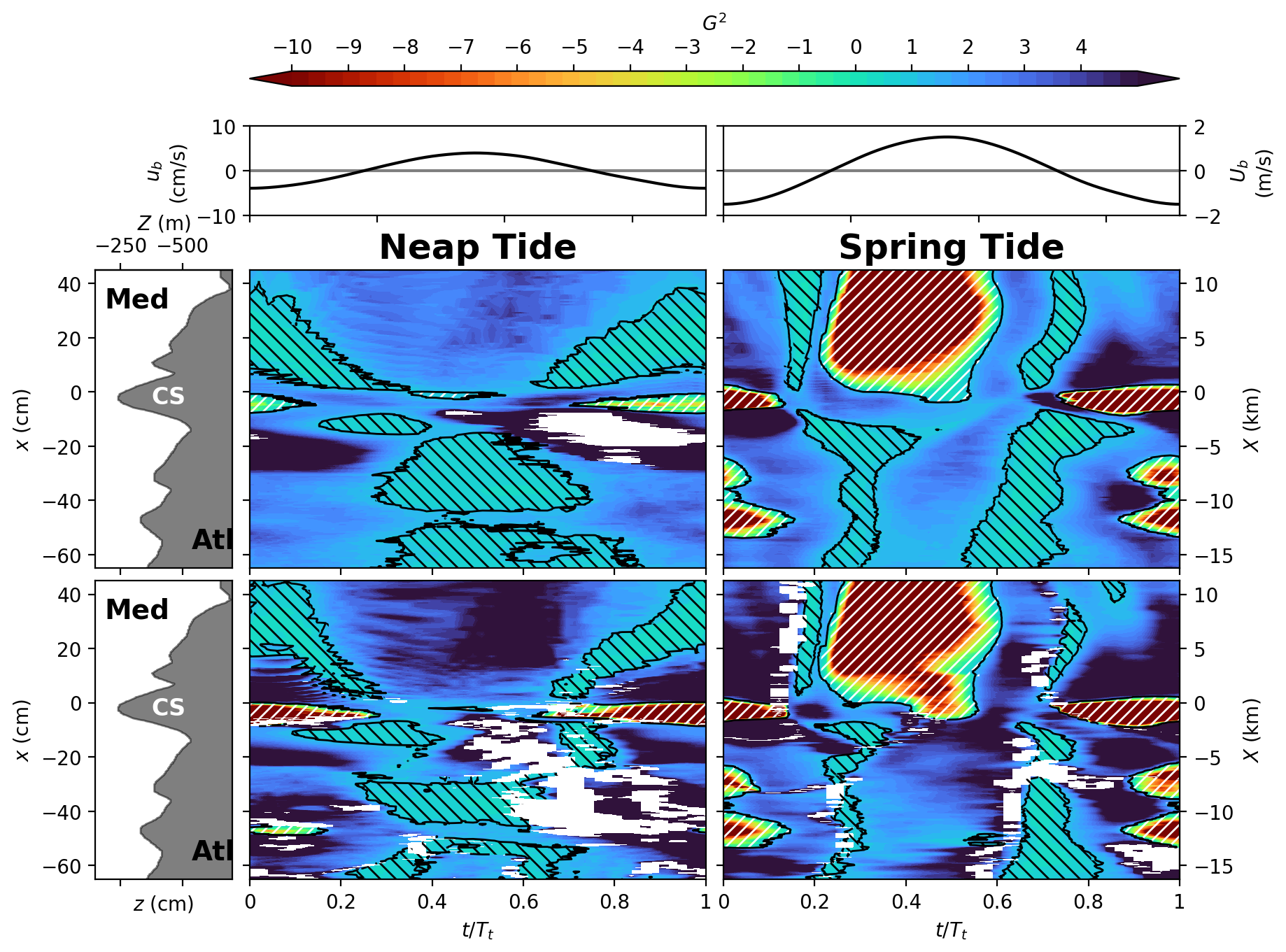
Figure E2 Comparison between the three-layer model proposed by Sannino et al. (2007), in which the layers are defined based on the density anomaly (${\mathit{\rho }}^{*}=\mathrm{0.25}$ and ${\mathit{\rho }}^{*}=\mathrm{0.75}$, top panels), and our model, in which the three layers are defined based on the depths corresponding to the maximum shear (S_max) and the maximum density gradient (N_max, bottom panels), for neap tides (left panels) and spring tides (right panels). The black contours indicate the condition G²=1. Regions with downward-sloping hatches correspond to areas where both modes are subcritical, while regions with upward-sloping hatches represent areas where both modes are supercritical. Blue-shaded areas indicate regions where only one of the two modes is supercritical, the other remaining subcritical. White areas correspond to regions where no third layer is defined.

Differences are more evident during neap tides, particularly regarding the persistence of control at CS throughout the tidal cycle. In the last left-hand panel of Fig. E1, corresponding to the calculation with a local g^′ and the depth at S_max, control at Camarinal is almost permanent, except for 2 % of the tidal cycle. In contrast, when the pycnocline is defined at ${\mathit{\rho }}^{*}=\mathrm{1}/\mathrm{2}$, approximately equivalent to N_max, the loss of control occurs over about 10 % of the tidal cycle.

When considering a three-layer system, multiple states are possible due to the presence of two modes that can propagate within the two intermediate layers. One can then distinguish a region where both modes are supercritical, a region where both are subcritical, and an intermediate region where one mode is subcritical while the other is supercritical (Sannino et al., 2007). The three-layer composite Froude number G² is defined as

$$\begin{array}{}\text{(E1)}& \begin{array}{rl}{G}^{\mathrm{2}}& ={\mathit{Fr}}_{\mathrm{1}}^{\mathrm{2}}+{\displaystyle \frac{{\mathit{Fr}}_{\mathrm{2}}^{\mathrm{2}}}{r}}+{\mathit{Fr}}_{\mathrm{3}}^{\mathrm{2}}-{\mathit{Fr}}_{\mathrm{1}}^{\mathrm{2}}{\mathit{Fr}}_{\mathrm{2}}^{\mathrm{2}}-{\mathit{Fr}}_{\mathrm{1}}^{\mathrm{2}}{\mathit{Fr}}_{\mathrm{3}}^{\mathrm{2}}\\ & -{\displaystyle \frac{\mathrm{1}-r}{r}}{\mathit{Fr}}_{\mathrm{2}}^{\mathrm{2}}{\mathit{Fr}}_{\mathrm{3}}^{\mathrm{2}},\end{array}\end{array}$$

where ${\mathit{Fr}}_{\mathrm{1}}=u_{\mathrm{1}}/\sqrt{g_{\mathrm{21}}^{\prime }{h}_{\mathrm{1}}}$, ${\mathit{Fr}}_{\mathrm{2}}=u_{\mathrm{2}}/\sqrt{g_{\mathrm{32}}^{\prime }{h}_{\mathrm{2}}}$, ${\mathit{Fr}}_{\mathrm{3}}=u_{\mathrm{3}}\sqrt{g_{\mathrm{32}}^{\prime }{h}_{\mathrm{3}}}$ with $g_{\mathrm{21}}^{\prime }=g({\mathit{\rho }}_{\mathrm{2}}-{\mathit{\rho }}_{\mathrm{1}})/{\mathit{\rho }}_{\mathrm{0}}$, $g_{\mathrm{32}}^{\prime }=g({\mathit{\rho }}_{\mathrm{3}}-{\mathit{\rho }}_{\mathrm{2}})/{\mathit{\rho }}_{\mathrm{0}}$ and $r=({\mathit{\rho }}_{\mathrm{2}}-{\mathit{\rho }}_{\mathrm{1}})/({\mathit{\rho }}_{\mathrm{3}}-{\mathit{\rho }}_{\mathrm{1}})$ (Smeed, 2000; Sannino et al., 2009). The doubly subcritical regime corresponds to

$$\begin{array}{}\text{(E2)}& {\displaystyle }{G}^{\mathrm{2}}<\mathrm{1}\text{and}{\mathit{Fr}}_{\mathrm{3}}^{\mathrm{2}}<{\displaystyle \frac{\mathrm{1}-r{\mathit{Fr}}_{\mathrm{1}}^{\mathrm{2}}}{\mathrm{1}-r}}.\end{array}$$

The doubly supercritical regime corresponds to

$$\begin{array}{}\text{(E3)}& {\displaystyle }{G}^{\mathrm{2}}<\mathrm{1}\text{and}{\mathit{Fr}}_{\mathrm{3}}^{\mathrm{2}}>{\displaystyle \frac{\mathrm{1}-r{\mathit{Fr}}_{\mathrm{1}}^{\mathrm{2}}}{\mathrm{1}-r}}.\end{array}$$

The comparison between the three-layer model proposed by Sannino et al. (2007), in which the layers are defined from the density anomaly (${\mathit{\rho }}^{*}=\mathrm{0.25}$ and ${\mathit{\rho }}^{*}=\mathrm{0.75}$, top panels), and our model, in which the three layers are defined from the depths corresponding to the maximum velocity shear (S_max) and maximum density gradient (N_max) (bottom panels), for neap tides (left panels) and spring tides (right panels), is presented in Fig. E2. The black contours indicate the condition G²=1. Regions with downward-sloping hatching correspond to areas where both modes are subcritical, whereas regions with upward-sloping hatching correspond to areas where both modes are supercritical. Blue regions indicate areas where only one of the two modes is supercritical, the other remaining subcritical.

Overall, we observe that our method and that of Sannino et al. (2007) show negligible differences during spring tides. For neap tides, the main difference concerns the duration of control at Camarinal: our model indicates control is maintained for approximately 75 % of the tidal cycle, compared to barely 50 % in the Sannino et al. (2007) model. Another difference is the appearance of a second control point at $x=-\mathrm{45}$ cm in our model, which is absent in Sannino et al. (2007).

These results remain consistent when considering the two-layer model. During spring tides, all models predict three control zones, at Camarinal and at the two western sites ($x=-\mathrm{20}$ and $x=-\mathrm{45}$ cm) during the outflow, while control is lost at Camarinal for approximately 45 %–55 % of the tidal cycle around the inflow, with a supercritical zone forming east of the sill. During neap tides, control at Camarinal is maintained for at least 50 % of the cycle using Sannino et al.'s three-layer model, 65 % with the two-layer model using a constant g^′ and ${\mathit{\rho }}^{*}=\mathrm{1}/\mathrm{2}$, and up to 88 %–98 % with the two-layer model using a local g^′ and a pycnocline defined by N_max or S_max.

In conclusion, we propose adopting the two-layer method with a local g^′. For comparison with the literature, it is possible to retain the definition of the pycnocline as the intermediate density value (${\mathit{\rho }}^{*}=\mathrm{1}/\mathrm{2}$, approximately equivalent to N_max), although the definition based on S_max also remains valid.