Phytoplankton blooms affect microscale differences of oxygen and temperature across the sea surface microlayer

The sea surface microlayer (SML) is the thin layer on top of the ocean that is in direct contact with the atmosphere and is crucial for air–sea interactions. Its properties are influenced in particular by surface-active substances (surfactants), mainly produced by phytoplankton and bacteria. Thus, phytoplankton blooms and their decay can have a considerable influence on the SML. A mesocosm study was conducted to assess the impact of a phytoplankton bloom on the SML using a multidisciplinary approach, which enabled in situ measurements under controlled yet natural conditions. A phytoplankton bloom was induced within a mesocosm facility filled with seawater, resulting in three phases of the study: the pre-bloom, bloom, and post-bloom phases. During all phases, microsensors measured in situ microprofiles of oxygen and temperature with a 125 µm vertical resolution through the air, SML, and underlying water. Microscale oxygen and temperature differences were determined from the profiles, as well as the thicknesses of the oxygen diffusion boundary layer (DBL) and thermal boundary layer (TBL). The night-time oxygen differences (Ø${}_{\mathrm{\Delta }{\mathrm{O}}_{\mathrm{2}},\text{pre-bloom}}$ = −2.16 ± 5.53 µmol L⁻¹, Ø${}_{\mathrm{\Delta }{\mathrm{O}}_{\mathrm{2}},\text{bloom}}$ = +24.90 ± 14.51 µmol L⁻¹, Ø${}_{\mathrm{\Delta }{\mathrm{O}}_{\mathrm{2}},\text{post-bloom}}$ = +2.07 ± 4.82 µmol L⁻¹) correlated highly with the chlorophyll a concentration (r = 0.755, p < 0.001), while the DBL thickness (Ø_{DBL, overall} = 937 ± 369 µm) showed a moderate correlation to the SML surfactant concentration (r = 0.490, p = 0.014). Both indicate the phytoplankton bloom's influence on oxygen differences across the SML. Night-time temperature differences (Ø_{ΔT, overall} = −0.133 ± 0.079 °C) and the TBL thickness (Ø_{TBL, overall} = 1300 ± 392 µm) were not correlated to the chlorophyll a or surfactant concentration. The mesocosm study and the microprofiling approach provide in situ data on the air–sea exchange processes in the SML, reflecting the distinct interplay of the SML and phytoplankton blooms in the exchange of oxygen and heat. This has implications for future studies on air–sea gas and heat exchange between the ocean and the atmosphere.

1 Introduction

The sea surface microlayer (SML) is of global importance as the layer that covers all oceans. Less than 1 mm thick, it forms the direct boundary between the atmosphere and the ocean (Cunliffe et al., 2013). This thin boundary layer is critical for the exchange of heat, momentum, gases, freshwater, and aerosols (Cunliffe et al., 2013; Wurl et al., 2016; Engel et al., 2017; Wong and Minnett, 2018; Cronin et al., 2019; Gassen et al., 2024; Laxague et al., 2024). A distinct SML covers large areas of the ocean under typical wind conditions and can therefore significantly influence processes such as global air–sea gas or heat exchange (Wurl et al., 2011, 2016, 2017). It accumulates biomass, in particular surface-active substances (i.e., surfactants) (Wurl et al., 2016), and serves as a unique habitat for microorganisms (Stolle et al., 2010; Cunliffe et al., 2013) and as a nursery ground for several species like crustaceans, molluscs, and fishes (Gallardo et al., 2021).

Slicks are an extreme form of the SML, covering approximately 30 % of coastal and 11 % of oceanic regions (Romano, 1996). They have a thicker viscous sublayer that dampens capillary waves and creates patches during calm water (Saunders, 1967; Katsaros, 1980). Physical and biological drivers, such as wind speed and primary production, play a crucial role in the formation and dispersion of slicks. The SML, enriched with surfactants including carbohydrates, proteins and lipids, harbours aggregates and gel-like particles exhibiting biofilm-like properties (Cunliffe et al., 2013; Wurl et al., 2016). Surfactants are produced by phytoplankton and heterotrophic bacteria in the SML or the underlying water (ULW), and are transported to the SML through rising air bubbles or buoyant particles (Žutić et al., 1981; Wurl et al., 2009; Kurata et al., 2016; Wurl et al., 2016). Heterotrophic activities in the SML are crucial for the formation and retention of slicks (Stolle et al., 2010; Wurl et al., 2016). Events such as phytoplankton blooms can increase surfactant concentrations, thereby leading to the formation of slicks (Sieburth and Conover, 1965; Wurl et al., 2018; Barthelmeß and Engel, 2022). By dampening surface waves, slicks significantly reduce air–sea heat and gas exchange fluxes (Katsaros, 1980; Laxague et al., 2024), for example, reducing global air–sea CO₂ fluxes by 19 % (Mustaffa et al., 2020).

Although the SML has distinct properties that differ from those of the ULW (Hunter, 1997), its thickness is difficult to determine because it is typically less than 1 mm and strongly influenced by environmental factors influencing near-surface turbulence, such as wind speed and surfactant concentration (Wurl et al., 2011, 2017). In field studies, the SML thickness is often defined operationally by the thickness of the layer that a sampling device can skim off the water surface. This approach does not necessarily represent the real thickness, and sampled thicknesses depend on the sampling device and vary between 10 and 250 µm (Falkowska, 1999). For the well-established glass plate method, sampled thicknesses agree well with the SML thickness of 50 µm, proposed through changes in chemical surface properties, but may vary from 40 to 100 µm (Harvey and Burzell, 1972; Zhang et al., 1998; Falkowska, 1999; Engel and Galgani, 2016).

Due to these difficulties in directly investigating the SML, other surface sub-layers are often considered. These sublayers include the diffusion boundary layer (DBL) of gases, such as oxygen or CO₂, and the thermal boundary layer (TBL) of temperature. Methods for determining the DBL thickness often rely on indirect measurements of gradients of dissolved gases. Carbon dioxide flux measurements were used to infer that the DBL thickness is approximately 50 µm (Robertson and Watson, 1992). The more recent application of microsensors has allowed for direct measurements of the DBL thickness of oxygen between 350 and 1100 µm (Rahlff et al., 2019; Adenaya et al., 2021). For determining the TBL, the sea surface temperature is typically measured using infrared radiometers and compared to subsurface temperatures. These measurements enable the calculation of both the surface temperature difference and the theoretical TBL thickness (Saunders, 1967). Surface temperature differences can range from +1.5 to −0.6 °C, but under common oceanic conditions, a cool skin layer with differences typically between −0.1 and −0.2 °C is observed due to a net heat loss at the ocean's surface (Ewing and McAlister, 1960; Robertson and Watson, 1992; Donlon et al., 1999; Murray et al., 2000; Donlon et al., 2002; Minnett et al., 2011). Reported TBL thicknesses can reach 8 mm (Ginzburg et al., 1977), but generally refer to the upper 1 mm (Donlon et al., 2002) and are highly dependent on the wind speed (Ward and Donelan, 2006).

Mesocosm experiments offer an optimal compromise between controlled laboratory conditions and natural field environments, allowing for the resolution of the dimensions of the SML (Galgani et al., 2014). They enable the mechanistic understanding of processes through the application of technology that is not applicable in open ocean settings. In this study, we induced a phytoplankton bloom in a mesocosm setting to assess its effects on the SML and ULW in a multidisciplinary study (Bibi et al., 2025a). To investigate the effect the bloom has on the DBL and TBL, we applied a novel method to obtain high-resolution in situ measurements of the oxygen concentration and temperature across the SML. Using a microprofiler equipped with microsensors, we continuously obtained in situ microprofiles of oxygen concentration and temperature from the air across the DBL/TBL into the ULW. We analysed night-time data without wind to ensure a focused assessment of the phytoplankton bloom's influence, independent of turbulent conditions or diurnal warming effects. The analysis of microprofiles provides in situ measurements of oxygen and temperature differences, oxygen exchange rates, and DBL and TBL thicknesses, while assessing the impact of the bloom. To our knowledge, this approach provides the first real DBL and TBL thicknesses representative of calm water masses at night conditions.

2 Methods

2.1 The mesocosm study

The mesocosm study was conducted between 15 May and 16 June 2023 at the Sea sURface Facility (SURF), located at the Institute for Chemistry and Biology of the Marine Environment (ICBM) in Wilhelmshaven, Germany (Bibi et al., 2025a). SURF is an 8.5 m × 2.0 m × 0.8 m large basin with a retractable roof, which can be filled with seawater from the Jade Bay, North Sea (Gassen et al., 2024). The multidisciplinary mesocosm study, part of the Biogeochemical processes and Air–sea exchange in the Sea–Surface microlayer (BASS) project, aimed to investigate the effects of a phytoplankton bloom on processes in the SML and is described in detail by Bibi et al. (2025a). The mesocosm was filled with filtered and skimmed seawater to remove suspended particles. Flow pumps at the bottom of the basin slightly mixed the ULW, resulting in a horizontally uniform water body and preventing particles and organisms from settling on the bottom. Through the addition of different nutrients on 26 May, 30 May, and 1 June, a phytoplankton bloom was induced.

As part of this multidisciplinary approach, various properties of the SML and ULW were recorded. Water temperature and salinity were measured using two conductivity–temperature–depth (CTD) sensors (48M; Sea and Sun Technology, Germany) at depths of approximately 2 and 40 cm below the surface. Discrete water samples from the SML and ULW were collected daily. To account for diurnal changes, sampling alternated between one hour after sunrise and ten hours after sunrise (Bibi et al., 2025a). SML samples were collected using the glass plate method of Harvey and Burzell (1972), while ULW samples at 40 cm depth were collected with a syringe attached to a tube (Bibi et al., 2025a). Subsamples of these samples were subsequently analysed for different parameters.

Surfactant concentrations in the SML and ULW, as concentrations of Triton equivalent (Teq), were measured in discrete samples using a Voltammetry technique (797 VA Computrace, including 863 Compact Autosampler, Metrohm, Switzerland) with a hanging drop mercury electrode (Ćosović and Vojvodić, 1987). The chlorophyll a concentration in the ULW (at 40 cm depth) was measured continuously using a FerryBox (-4H-Jena PocketBox, 4H Jena Engineering, Germany), which also measured oxygen concentration, temperature, and salinity. The FerryBox oxygen concentration was corrected with daily discrete samples analysed with the Winkler method (see Appendix B). Chlorophyll a measurements were corrected using discrete water samples. Bacterial abundances in the SML and ULW were measured in discrete samples. A comprehensive description of all these methods and the biogeochemical dynamics throughout the study can be found in Bibi et al. (2025a). Discrete samples of phytoplankton and protozooplankton were analysed from 250 mL Lugol-fixed samples by AquaEcology GmbH & Co. KG. For abundance determination, the samples were transferred to sedimentation chambers and allowed to settle overnight (Utermöhl, 1958; DIN, 2011). Individual cells were then counted under an inverted microscope (100×, 200× and 400× magnification). If possible, organisms were identified to species level or otherwise assigned to the genus or a higher taxonomic level.

2.2 The microprofiler setup

Continuous microprofiles across the SML were acquired using one oxygen (OX-200) and two temperature (TP-200) microsensors mounted on a MicroProfiling System (UNISENSE, Denmark) (Fig. 1). The microsensors were fast responding, exhibited minor drift over time and had a low stirring sensitivity. The oxygen microsensor possessed a detection limit of 0.3 µmol L⁻¹, and the resolution of the temperature microsensor was 0.1 °C. The oxygen microsensor measured the oxygen partial pressure in the air and water and converted it to an oxygen concentration which was accurate for the water without changing the shape of the microprofiles. The microsensors were mounted a few centimetres apart, with their tips facing upwards and close to the water surface, which was defined as a depth of 0 µm. To measure from the air, across the surface into the ULW, profiles were initiated at a height of 3000 µm in the air and descended to a depth of 7000 µm in the water, in increments of 125 µm, for optimal spatial and temporal resolution. At each step, the microsensors took three measurements with 50 Hz, each lasting 10 s, and recorded the mean and standard deviation before proceeding to the next step. The slow movement of the microprofiler ensured minimal artificial water flow and turbulence in proximity to the microsensors. Each profile took between 40 and 50 min, and profiling was performed continuously throughout the mesocosm study. To cover the time before, during and after the bloom, profiles from 22 May onward were further analysed. The transparent roof of SURF allowed the water to be exposed to natural diurnal variations in solar radiation. To reduce the effects of solar radiation and diurnal heating, only profiles from one hour after sunset to one hour before sunrise (approximately 22:30 to 04:00 local time) were analysed, yielding four to ten profiles per night and 141 in total. The roof of SURF was closed at night to exclude wind and rain effects, allowing examination of only the phytoplankton bloom's influence on oxygen concentration and temperature, and their differences across the SML. While the closed roof and walls prevented wind from freely blowing across the water surface, the interior of SURF continued to be affected by fluctuations in outside temperature due to heat transfer through the roof.

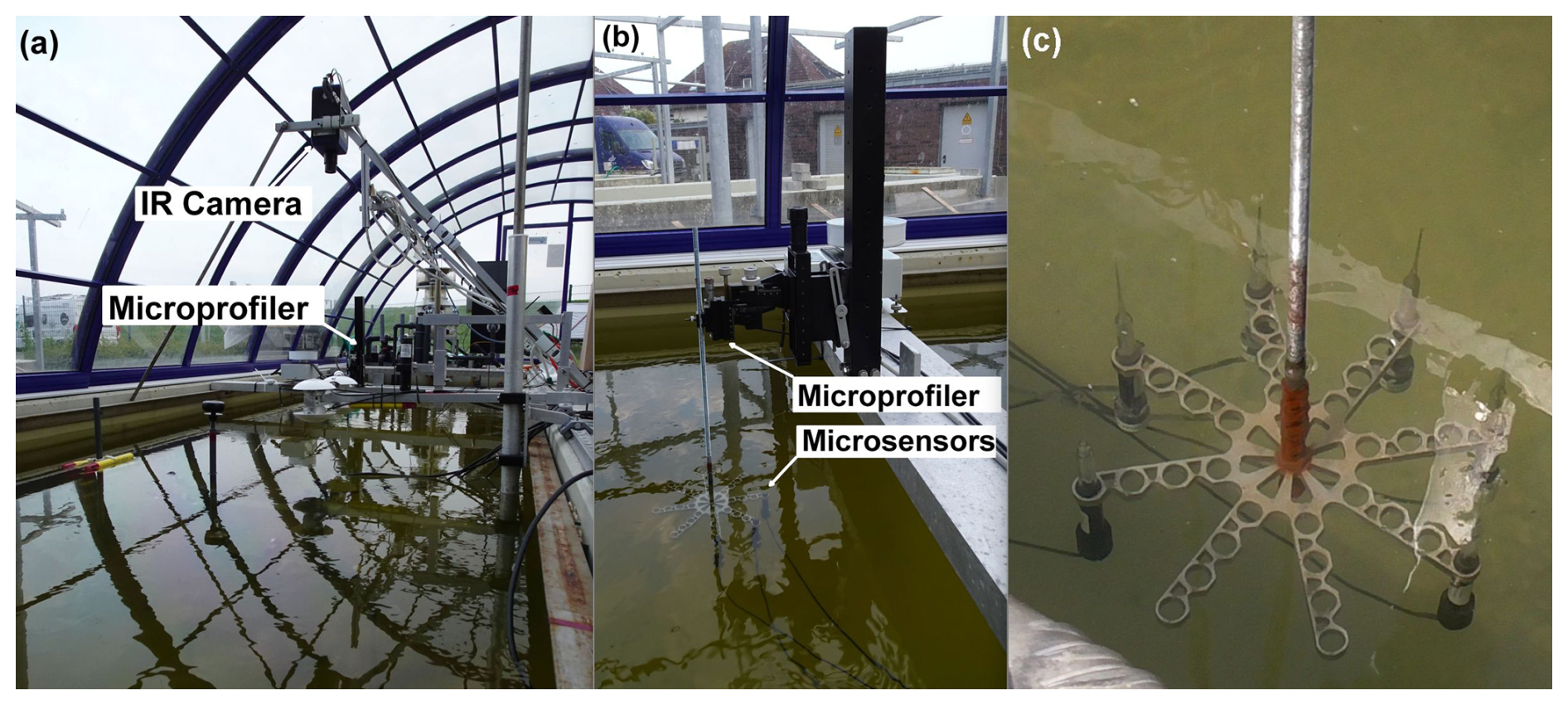
Figure 1 (a) Setup of different sensors inside SURF including the microprofiler and IR camera. (b) Microprofiler setup with microsensor array. (c) Close-up image of the microsensors and holder used during the mesocosm study.

The oxygen microsensor was calibrated before the study to ensure consistent data. Potential biases compared to a daily calibrated sensor were assessed separately, with no consistent offset being established (Appendix A). Furthermore, the microsensor measurements were compared to oxygen measurements of the FerryBox, and biases were minimal or explainable by oxygen gradients across the ULW (Appendix B). Our work focuses on the surface oxygen differences rather than absolute concentrations, prioritising data consistency for night-to-night comparability over absolute measurement accuracy. Based on the microprofiles, oxygen and temperature differences across the SML were calculated, along with the thicknesses of the oxygen DBL and TBL (Sect. 2.3 and 2.4). To compare the oxygen and temperature differences, as well as the DBL/TBL thicknesses, with chlorophyll a concentration and surfactant concentration, the mean of each parameter per night was calculated, checked for normality, and examined for correlation using a Spearman correlation analysis. This analysis shows the correlation between non-normally distributed variables, with a correlation coefficient r > 0.7 and a p-value < 0.05 indicating strong correlations, 0.4 < r < 0.7 and 0.05 < p < 0.10 indicating moderate correlations and r < 0.4 and p > 0.10 indicating weak or no correlations.

2.3 Determination of the diffusion boundary layer

To determine the DBL thickness and the oxygen differences across the DBL, the mean of the triplicates at each depth was calculated (Fig. 2). The microprofiler's 0 µm depth (nominal air–water interface) did not necessarily reflect the sensor tip's true position, as manual alignment of multiple sensors introduced minor vertical offsets (−371 ± 1292 µm), which were corrected in our analysis. Six points (P1–6) in the profile were manually assigned. P1 and P2 were in the air above a sharp gradient, which indicated the location of the water surface. P2 was selected near the water surface, with a nearly linear trend between P1 and P2. P3 and P4 marked the upper and lower ends of the DBL, respectively. The DBL could be found by a large oxygen concentration gradient or by enhanced standard deviations and different gradients compared to the air and the ULW. P5 and P6 were assigned to the ULW below the sharp DBL gradient, where a linear downward trend was present.

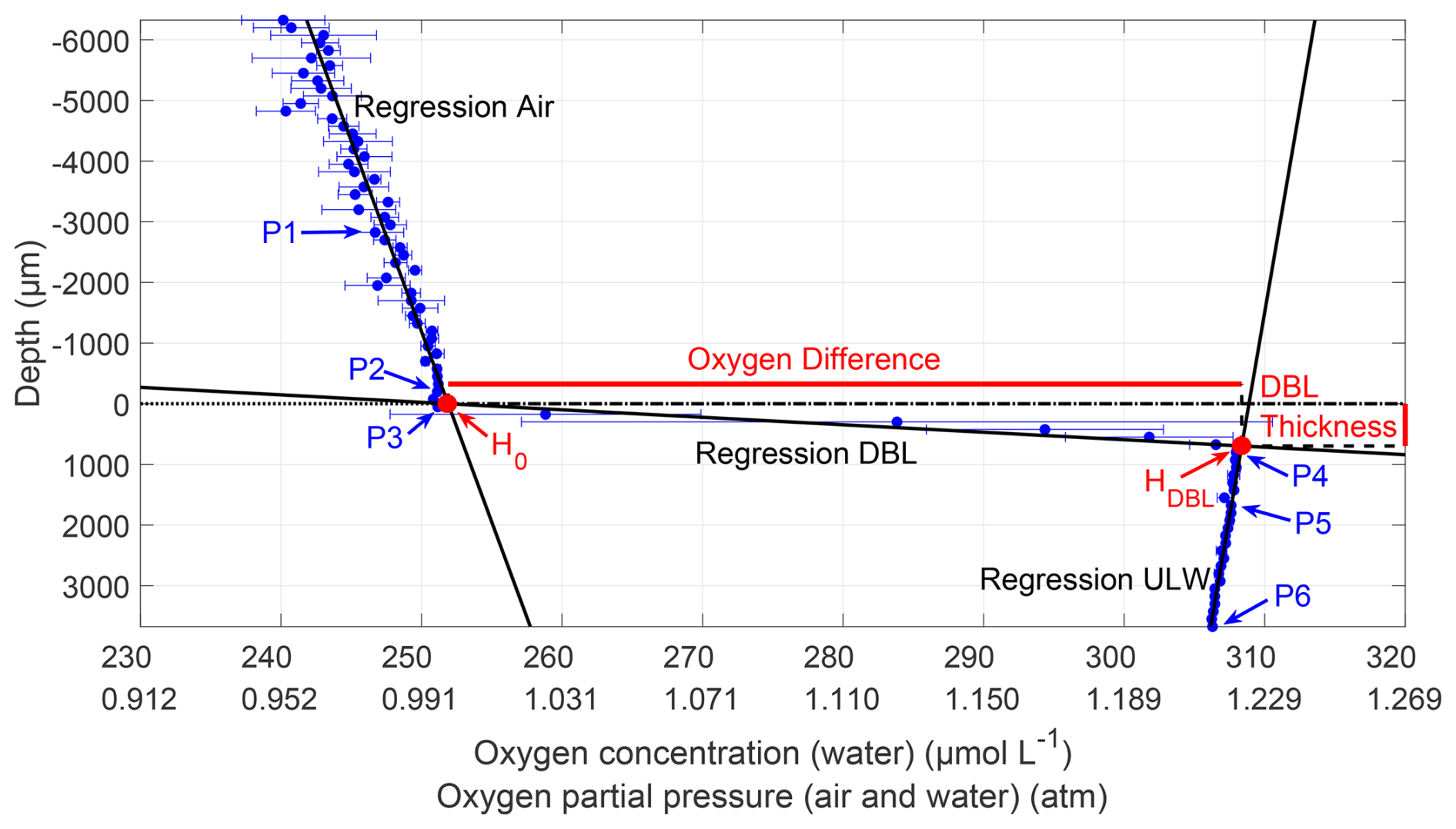
Figure 2 Microprofile of the oxygen concentration (31 May 2023, Profile 2). The oxygen concentration is accurate for the water profile but not for the air profile; the oxygen partial pressure is accurate for both profiles. Depth corrected for the proper sensor position; 0 µm indicates the air–water interface (dotted line); points P1–P6 were used to calculate regressions for air, DBL, and ULW. The intersection of air and DBL regression H₀ is the upper position of the water surface, and the intersection of DBL and ULW regression H_DBL is the lower DBL boundary. The vertical difference between H_DBL and H₀ represents the DBL thickness, and the horizontal difference represents the oxygen difference across the DBL.

Based on Rahlff et al. (2019), three linear regressions were computed with all measurements between the pairs P1 and P2, P3 and P4, and P5 and P6. The intersection between the air (P1 and P2) and DBL (P3 and P4) regression lines was the upper position of the water surface H₀. The intersection between the regression lines of DBL and ULW (P5 and P6) was the depth of the lower boundary of the DBL (H_DBL). The difference in depth between H_DBL and H₀ was the DBL thickness, and the difference in oxygen concentration between H_DBL and H₀ was the oxygen difference across the DBL. A positive difference indicated higher oxygen concentrations in the ULW than in the air.

2.4 Determination of the thermal boundary layer

The analysis of the temperature microprofiles followed the same steps as the oxygen microprofile analysis (Fig. 3). The difference between the TBL and ULW was apparent in the profiles, as the TBL showed a pronounced temperature gradient. In contrast, the temperature in the ULW remained nearly constant with depth. To differentiate the air and TBL, which had similar temperature trends, the standard deviation at each step in the profile was considered. Temperatures across the TBL were less variable than air temperatures, exhibiting apparent differences in standard deviations. This was used to identify the change from air to TBL and aided in assigning points P2 and P3. The TBL thickness was calculated as the difference between the depth of the lower boundary of the TBL H_TBL and the upper position of the water surface H₀; and the temperature difference across the TBL was the difference between the temperatures at H₀ and H_TBL. Contrary to the oxygen profiles and due to the nomenclature referring to a “cool skin layer” (Robertson and Watson, 1992; Soloviev and Schüssel, 1994; Wurl et al., 2018; Yan et al., 2024), a negative temperature difference refers to a cooler upper boundary than lower boundary of the TBL.

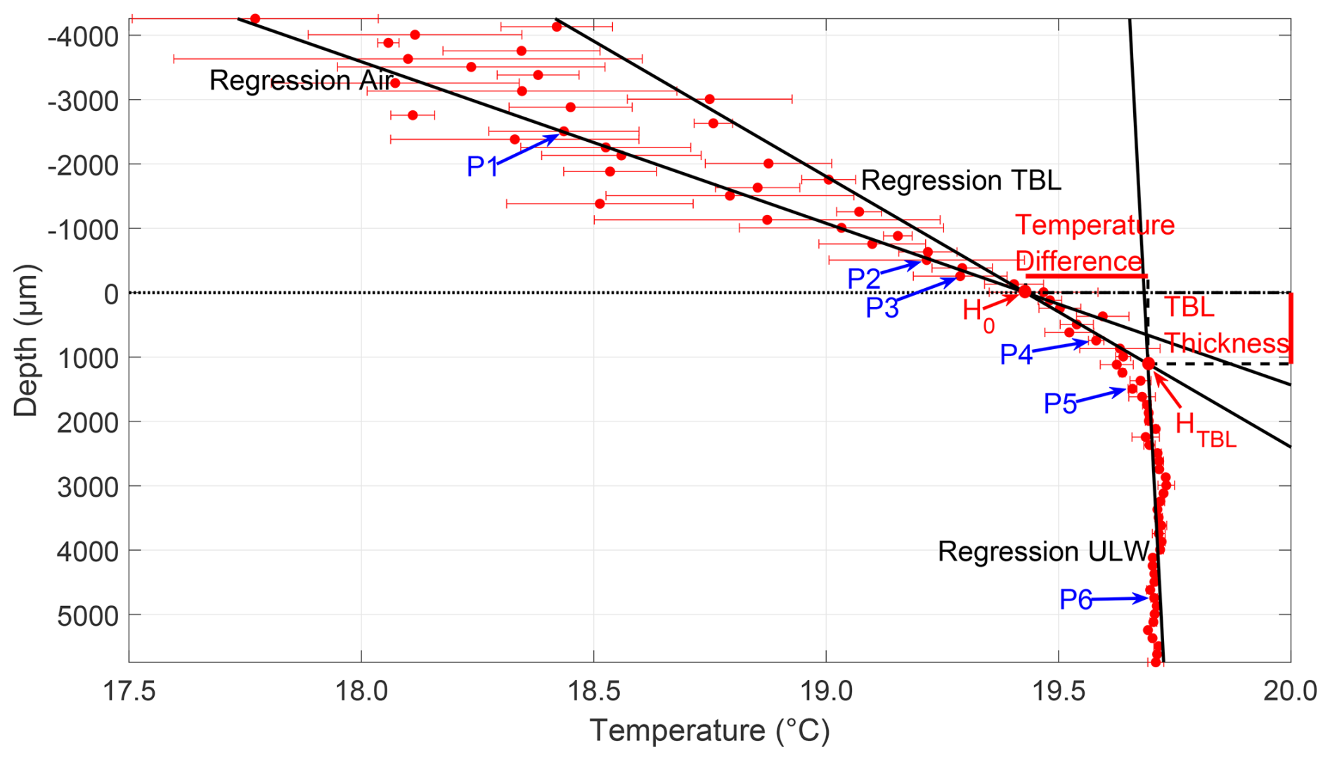
Figure 3 Microprofile of the temperature (31 May 2023, Profile 1). Depth corrected for the proper sensor position; 0 µm indicates air–water interface (dotted line); points P1–P6 were used to calculate the regressions for air, TBL, and ULW. The intersection of air and TBL regression H₀ is the upper position of the water surface, and the intersection of TBL and ULW regression H_TBL is the lower TBL boundary. The vertical difference between H_TBL and H₀ represents the TBL thickness, and the horizontal difference represents the temperature difference across the TBL.

2.5 Determination of the gas exchange rate

The oxygen microprofiles were used to calculate the gas exchange rate, which represents the overall decline of oxygen at the lower end of the DBL. It was calculated after Eq. (1) by Goldman et al. (1988)

$$\begin{array}{}\text{(1)}& K={\displaystyle \frac{V}{A}}\cdot {\displaystyle \frac{\mathrm{1}}{\mathrm{\Delta }t}}\cdot \ln \left({\displaystyle \frac{C_{\mathrm{0}}}{C_t}}\right)\end{array}$$

where K [cm h⁻¹] is the gas exchange rate, V [cm³] is the water volume and A [cm²] the surface area of SURF, C₀ [µmol L⁻¹] is the oxygen concentration at H_DBL in the first profile of the night, C_t [µmol L⁻¹] is the oxygen concentration at H_DBL in the last profile of the night, and Δt [h] is the time difference between the first and last profile. One gas exchange rate was calculated per night. Furthermore, the oxygen saturation of the water was calculated (Appendix C). To assess the phytoplankton bloom's impact on the gas flux between water and air, the diffusive rate was calculated (Appendix D). The diffusive rate indicates oxygen exchange between water and air for each profile, while the gas exchange rate represents the overall loss of oxygen in the water per night.

2.6 Horizontal temperature measurements with an infrared camera

Infrared (IR) imagery is capable of resolving horizontal temperature features across small eddies or slick edges (Marmorino et al., 2018). While studies of horizontal surface temperature gradients span local to global scales (Katsaros and Soloviev, 2004; Tozuka et al., 2018; Wurl et al., 2018; Zappa et al., 2019), analyses of the surface temperature on centimetre scales are mainly conducted in laboratory setups (Saylor et al., 2000; Flack et al., 2001; Saylor et al., 2001; Veron and Melville, 2001; Jessup et al., 2009; Wells et al., 2009). A FLIR SC7750-L infrared camera (Teledyne FLIR LLC, USA) was used to record horizontal small-scale temperature structures during this study. The camera, mounted near the microsensors, which were positioned just outside the field of view, provided a resolution of 640 × 512 pixels, with each pixel covering an area of 1.657 mm × 1.586 mm, and a total field of view of 1.061 m × 0.812 m. Images were recorded at a rate of one image per second. While the absolute value had an accuracy of ±1 °C, horizontal temperature differences larger than 35 mK could be detected, as the noise equivalent temperature difference was greater than 35 mK. Due to reflections, a reference image was created for correction by calculating the median from 60 images, which was subtracted from each original image. A two-dimensional moving median filter was used to remove small outliers from each image. The filter determined the median for each pixel in the image by examining a 3×3 window of surrounding pixel values. This median then replaced the original pixel value, becoming the new output pixel.

3 Results

To assess the influence of the phytoplankton bloom on the oxygen diffusion boundary layer (DBL) and thermal boundary layer (TBL), we first illustrate examples of oxygen microprofiles from different phases of the bloom. Then, we present the oxygen differences and DBL thicknesses, comparing them to the concentrations of chlorophyll a and surfactants. Next, we present the gas exchange rate and its influence by the phytoplankton and bacterial blooms. We subsequently present the temperature differences and TBL thicknesses in comparison to the concentrations of chlorophyll a and surfactants. Finally, we give an example of an infrared camera image of the surface temperature to assess horizontal temperature gradients.

3.1 Oxygen microprofiles

The mesocosm study was categorised into three distinct phases based on the dynamics of the chlorophyll a concentration: the pre-bloom phase (18 to 26 May), the bloom phase, starting with the addition of nutrients until chlorophyll a reached levels to those prior to the addition (27 May to 4 June), and the post-bloom phase (5 to 16 June) (Bibi et al., 2025a). During the bloom and post-bloom phases, a slick was visually observed at the water surface. The presence of a slick was confirmed, as the surfactant concentration exceeded the slick threshold of 1000 µg L⁻¹ during the bloom and post-bloom phases (Bibi et al., 2025a; Wurl et al., 2011).

For the oxygen microprofiles during the nights of all bloom phases, the oxygen partial pressure in both the air and the water decreased from one profile to the next, with the larger decrease in the water (Fig. 4). During all nights, a gradient in oxygen partial pressure existed in the air, with higher partial pressures near the water surface. Typically, air gradients exceeded 0.02 atm over a few millimetres. In addition, the oxygen concentration decreased with depth in the ULW. To test, whether this decrease was due to depth or time, vertical rates were calculated, similar to the gas exchange rate in Sect. 2.5. Equation (1) was used, now with C₀ being the oxygen concentration at the point P5 and C_t the concentration at P6. Δt was the time difference between the measurements at P5 and P6. Until 6 June, the mean vertical rate for each night was similar to the overall gas exchange rate (Sect. 3.4) (differences of 0.038 ± 0.157 cm h⁻¹), indicating, that a decline over time mainly caused the decrease in oxygen concentration with depth in the ULW. However, in the post-bloom phase from 7 June onward, the vertical rate constantly exceeded the gas exchange rate (differences of 0.538 ± 0.375 cm h⁻¹), indicating a vertical oxygen gradient in the ULW that was not solely due to temporal decreases.

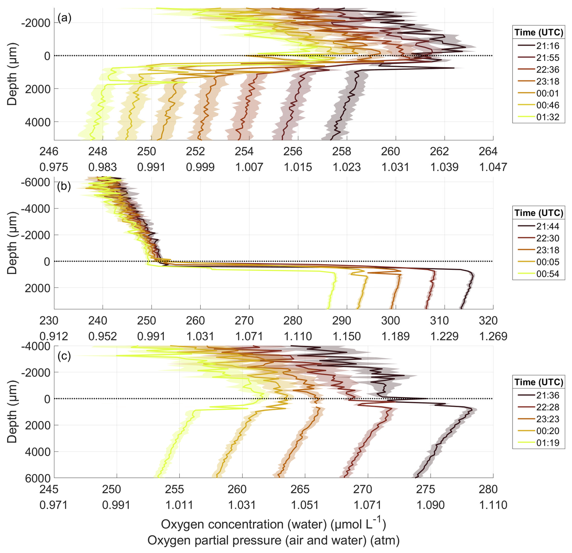
Figure 4 Oxygen microprofiles throughout the night of 22 May in the pre-bloom phase (a), 31 May in the bloom phase (b), and 11 June in the post-bloom phase (c), depth corrected for the proper sensor position. The oxygen concentration is accurate for the water profile but not for the air profile; the oxygen partial pressure is accurate for both profiles. 0 µm indicates the air–water interface (dotted line). Times are the mean times of the profile; one profile took between 40 and 50 min to complete.

On 22 May, before the bloom, the oxygen difference across the DBL was consistently negative. It intensified overnight with the oxygen concentration in the water decreasing by 10 µmol L⁻¹ (Fig. 4a). On 31 May, during the bloom, the oxygen difference across the DBL remained constantly positive (Fig. 4b). The oxygen concentration in the ULW was 48 µmol L⁻¹ higher than before the bloom. The decrease overnight of 28 µmol L⁻¹ was likewise greater. On 11 June, after the bloom, the oxygen concentration in the ULW was 36 µmol L⁻¹ lower than during the bloom, but 12 µmol L⁻¹ higher than before the bloom (Fig. 4c). The oxygen difference across the DBL shifted from positive to negative during the night and declined by 21 µmol L⁻¹.

3.2 Oxygen differences across the DBL

The oxygen differences exhibited a trend over time similar to that of the chlorophyll a concentration (Fig. 5). Before the bloom on 22 May, the chlorophyll a concentration was 1.5 µg L⁻¹, and the oxygen difference was negative, with a median of −6.81 µmol L⁻¹ and a low variability. After the induction of the bloom on 26 May, chlorophyll a increased and reached a maximum of 11.2 µg L⁻¹ on 2 June, while during the bloom, the oxygen differences and their variability also increased. On 31 May, a maximum difference of 49.48 µmol L⁻¹ was observed. As the chlorophyll a concentration declined in the post-bloom phase to background levels, oxygen differences also decreased to a minimum of −5.90 µmol L⁻¹, similar to pre-bloom levels, and stayed around zero in the later post-bloom phase. The mean oxygen difference over the entire study was +7.28 ± 15.98 µmol L⁻¹, but differences were evident when comparing the bloom phase to the pre-bloom and post-bloom phases. In the pre-bloom phase, the mean oxygen difference of −2.16 ± 5.53 µmol L⁻¹ was similar to that of the post-bloom phase (+2.07 ± 4.82 µmol L⁻¹), but differed significantly from the mean difference during the bloom (+24.90 ± 14.51 µmol L⁻¹). The oxygen differences showed a strong correlation with the chlorophyll a concentration (r=0.755, p<0.001). The oxygen differences were not significantly correlated with the surfactant concentration (r=0.215, p = 0.300), which started to increase at the bloom's peak and reached its maximum after the chlorophyll a and oxygen difference maxima. When a lagged correlation was calculated between oxygen differences and surfactant concentration with 3 d lag, the correlation strengthened significantly (r = 0.703, p < 0.001). Unless otherwise noted, other correlations did not significantly increase when lagged.

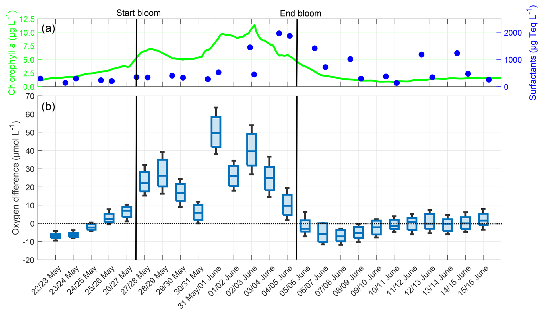
Figure 5 (a) ULW chlorophyll a concentration (green) and SML surfactant concentration (blue) between 22 May and 16 June, (b) Oxygen differences in the SML during the nights between 22 May and 16 June, 4–10 profiles per night, box: 25 % to 75 % quartile, horizontal line: median, whiskers: largest and smallest value. The dotted line indicates the zero level and the solid black lines indicate the start and end points of the bloom phase.

3.3 Oxygen diffusion boundary layer thickness

The thickness of the oxygen DBL showed a different trend than the oxygen differences (Fig. 6). In the pre-bloom phase, the median DBL thickness varied within a narrow range (680 to 939 µm). Towards the end of the bloom phase, the DBL thickness increased, probably due to elevated surfactant concentrations. The surfactant concentration reached its maximum of 1963 µg Teq L⁻¹ on 4 June, and the DBL thickness reached its maximum, with a median of 1483 µm on 6 June. Subsequently, the surfactant concentration and DBL thickness decreased but remained higher than in the pre-bloom phase. Overall, DBL thicknesses showed no correlation with the chlorophyll a concentration ($r=-\mathrm{0.115}$, p=0.584) or oxygen differences ($r=-\mathrm{0.272}$, p=0.187), but a moderate correlation with surfactant concentrations (r=0.490, p=0.014) was observed. Although the mean DBL thickness (mean entire study: 936.73 ± 369.49 µm) increased from the pre-bloom phase (831.61 ± 344.32 µm) to the bloom phase (911.81 ± 342.82 µm) and post-bloom phase (1012.31 ± 393.76 µm), this increase was not significant.

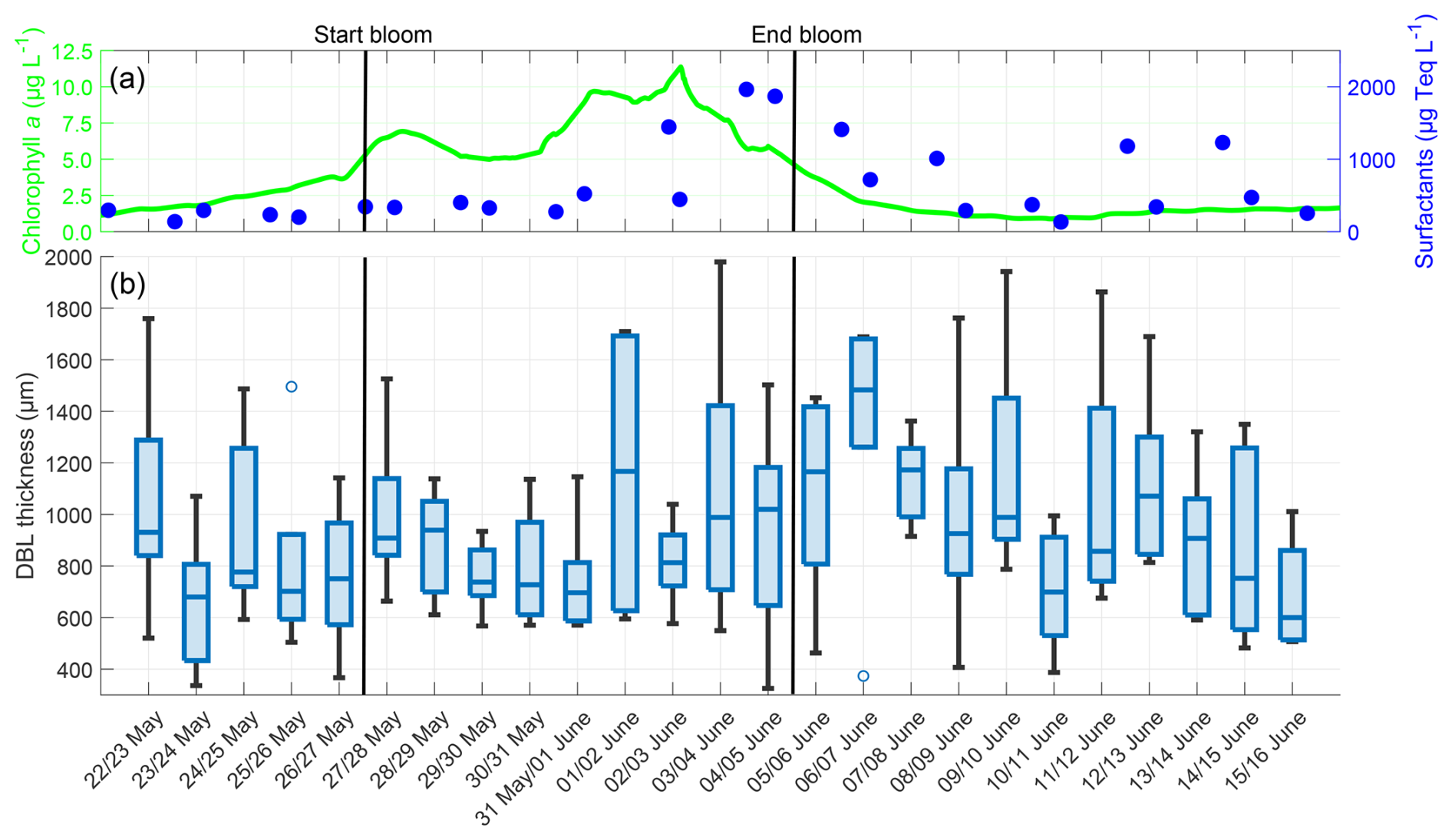
Figure 6 (a) ULW chlorophyll a concentration (green) and SML surfactant concentration (blue) between 22 May and 16 June, (b) Oxygen DBL thickness during the nights between 22 May and 16 June, 4–10 profiles per night, box: 25 % to 75 % quartile, horizontal line: median, whiskers: largest and smallest nonoutlier value, open circles: outliers (difference to next value >1.5 times interquartile range). The solid black lines indicate the start and end points of the bloom phase.

3.4 Gas exchange rate

The night-time gas exchange rate followed the trends of chlorophyll a concentration and phytoplankton abundance during the pre-bloom and bloom phases (Fig. 7). In the post-bloom phase, it appeared to be influenced by bacterial abundance. The phytoplankton abundance increased steadily until 3 June with a maximum of approximately 160×10⁶ cells L⁻¹, before it began to decline. The protozooplankton abundance began to increase after 31 May, reaching its maximum of 39×10⁶ cells L⁻¹ on 4 June. The bacterial abundances were 1.11×10⁹ cells L⁻¹ (SML) and 0.69×10⁹ cells L⁻¹ (ULW) on 22 May. There was a slight decrease in abundance during the bloom, but an increase in both the SML and ULW in the post-bloom phase, with their maxima on 14 June with 1.47×10⁹ cells L⁻¹ (SML) and 1.68×10⁹ cells L⁻¹ (ULW). The earlier increase in the ULW was partly caused by the release of dissolved organic matter in the ULW at the end of the phytoplankton bloom, which was consumed by the bacteria (Bibi et al., 2025a). The shift between SML and ULW can be explained by the presence and proportion of different bacterial groups. In the ULW, bacterial communities were already prevalent during the bloom phase and increased in abundance. In contrast, in the SML Gammaproteobacteria associated with the biofilm-like properties of the SML lead to a later increase in bacterial abundance (Athale et al., 2026; Rahlff et al., 2023).

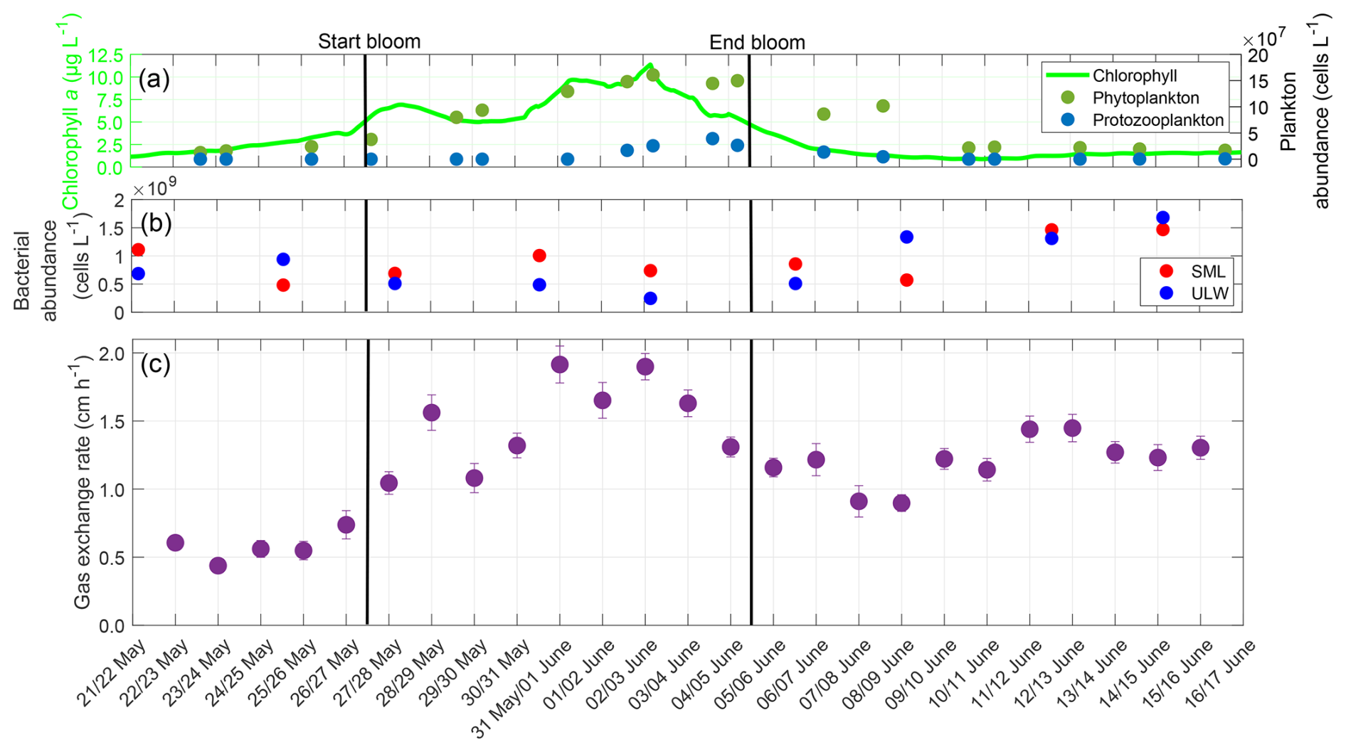
Figure 7 (a) ULW chlorophyll a concentration (green), phytoplankton abundance (dark-green), and protozooplankton abundance (blue) between 22 May and 16 June, (b) Bacterial abundance in the SML (red) and ULW (blue), (c) Mean gas exchange rate during the nights. The solid black lines indicate the start and end points of the bloom phase.

Before the bloom phase, the gas exchange rate reached its minimum at 0.44 cm h⁻¹ on 23 May, it then increased to a maximum of 1.91 cm h⁻¹ on 31 May during the bloom, before declining after the bloom to approximately 1.20 cm h⁻¹. The higher gas exchange rate in the post-bloom phase compared to the pre-bloom phase was accompanied by a higher bacterial abundance, both in the SML and ULW. In contrast, the phytoplankton abundances remained similar compared to pre-bloom levels. The mean gas exchange rate over the entire study was 1.21 ± 0.38 cm h⁻¹. In the pre-bloom phase, the mean gas exchange rate was 0.58 ± 0.11 cm h⁻¹, before increasing to 1.49 ± 0.32 cm h⁻¹ in the bloom phase, and then decreasing to 1.20 ± 0.18 cm h⁻¹ in the post-bloom phase. The gas exchange rate showed a moderate correlation with the phytoplankton abundance (r=0.559, p=0.004) and the surfactant concentration (r=0.588, p=0.002), but not with zooplankton abundance (r=0.324, p=0.114) or chlorophyll a concentration (r=0.384, p=0.059). With a 2 d lag, the correlation with the surfactant concentration increased to a strong and significant correlation (r=0.788, p<0.001), while with a 4 d lag, the correlation with the zooplankton abundance increased to a strong and significant correlation (r=0.857, p<0.001). The oxygen saturation followed a similar trend to the gas exchange rate, being influenced by both the phytoplankton and bacterial abundances (Appendix C). The diffusive rates exhibited a trend similar to that of the oxygen differences, with a significant increase during the bloom phase, but comparable levels in the pre-bloom and post-bloom phases (Appendix D).

3.5 Temperature differences across the TBL

The temperature microprofiles observed during the night appeared similar across all nights, regardless of the bloom phase, and an example of the profiles of both temperature microsensors on 22 May is given in Appendix E. The temperature differences across the TBL did not follow a trend for either sensor, neither in their median nor in their variability (Fig. 8). A cooler skin layer was always present, with negative temperature differences approaching −0.4 °C in extreme cases. There were no correlations between the temperature differences for both sensors and either the chlorophyll a concentration (Sensor 1: r=0.067, p=0.439; Sensor 2: $r=-\mathrm{0.077}$, p=0.374) or the surfactant concentration (Sensor 1: r=0.224, p=0.003; Sensor 2: $r=-\mathrm{0.084}$, p=0.331). The deviations in mean temperature differences between both sensors ranged from 0.001 to 0.142 °C, with a mean of 0.048 ± 0.036 °C. These deviations were not caused by measurement inaccuracies, but by small scale processes such as buoyancy fluxes. These processes alter the shape of the profiles locally and leading to a larger variability, as has also been observed in temperature microprofiles by Ward and Donelan (2006). High medians and interquartile ranges, such as on 29 May and 2 June, were caused by two outliers with a high temperature difference per night respectively, but do not indicate a general trend for higher temperature differences during the bloom phase. The mean temperature difference over the entire study, as measured by both combined sensors, was −0.133 ± 0.079 °C. No significant differences were found between the pre-bloom (−0.130 ± 0.073 °C), bloom (−0.137 ± 0.084 °C), and post-bloom (−0.132 ± 0.079 °C) phases.

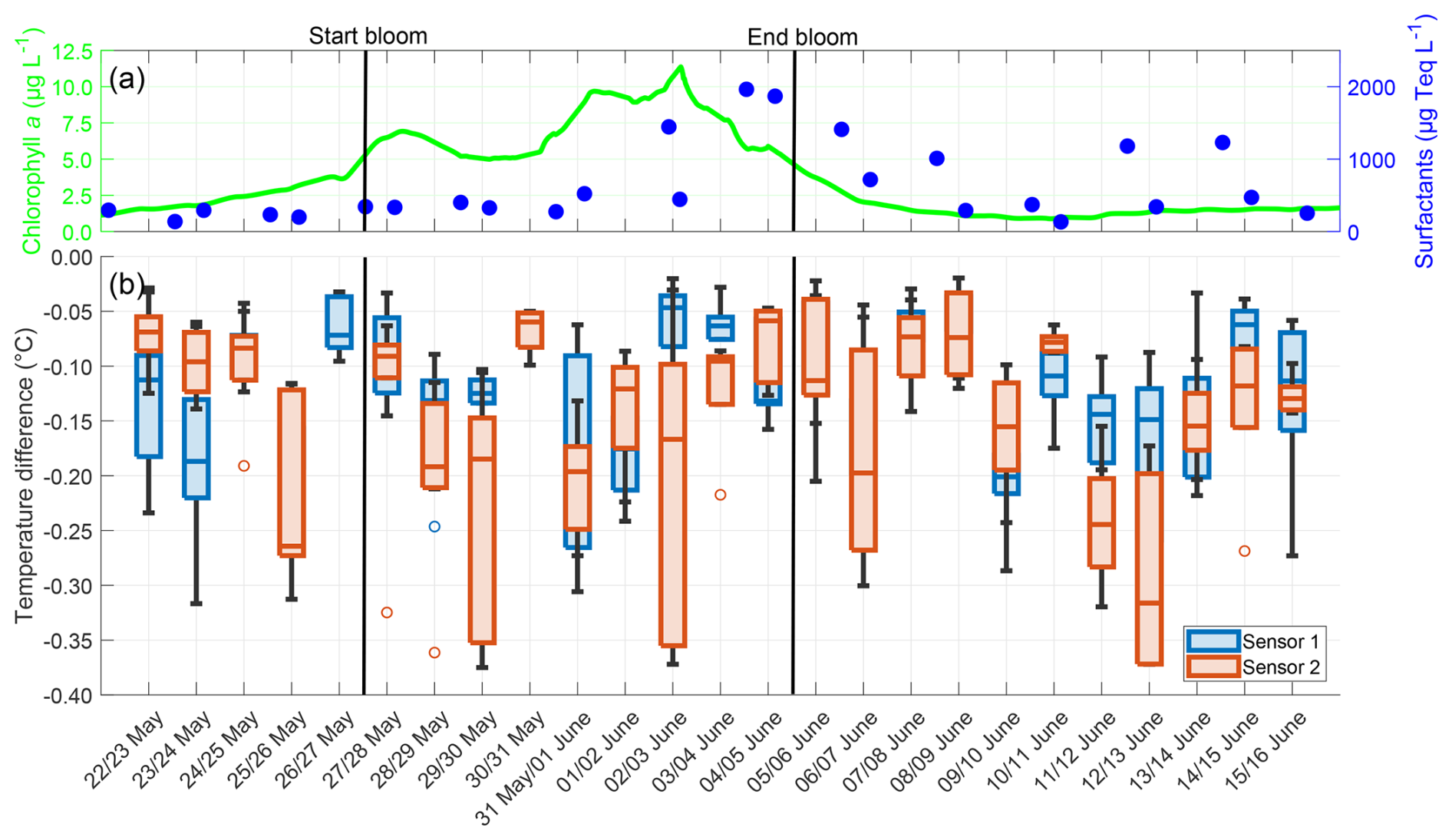
Figure 8 (a) ULW chlorophyll a concentration (green) and SML surfactant concentration (blue) between 22 May and 16 June, (b) Temperature differences from Sensor 1 (blue) and Sensor 2 (red) during the nights between 22 May and 16 June, 4–10 profiles per night, box: 25 % to 75 % quartile, horizontal line: median, whiskers: largest and smallest nonoutlier value, open circles: outliers (difference to next value >1.5 times interquartile range). The large interquartile range of Sensor 2 on 29 May and 2 June is caused by two outliers in these nights. The solid black lines indicate the start and end points of the bloom phase.

3.6 Thermal boundary layer thickness

The TBL thickness showed no trend but exhibited fewer extreme values than the temperature differences (Fig. 9). There was no correlation with the chlorophyll a concentration (Sensor 1: r = −0.100, p = 0.243, Sensor 2: r = −0.112, p = 0.195) or the surfactant concentration (Sensor 1: r = −0.082, p = 0.338; Sensor 2: r = 0.123, p = 0.153). However, the TBL thickness showed a moderate negative correlation with the temperature differences (Sensor 1: r = −0.453, p = 0.037; Sensor 2: r = −0.615, p = 0.002). The deviations in mean TBL thickness between the sensors ranged from 4.97 to 652.13 µm, with the mean deviation being 271.70 ± 190.71 µm. The mean TBL thickness over the entire study, as measured by both combined sensors, was 1299.50 ± 391.80 µm, being approximately 360 µm thicker than the oxygen DBL. There were no significant differences in the mean TBL thickness of the pre-bloom phase (1239.42 ± 342.76 µm), bloom phase (1277.09 ± 360.34 µm), and post-bloom phase (1348.41 ± 393.76 µm).

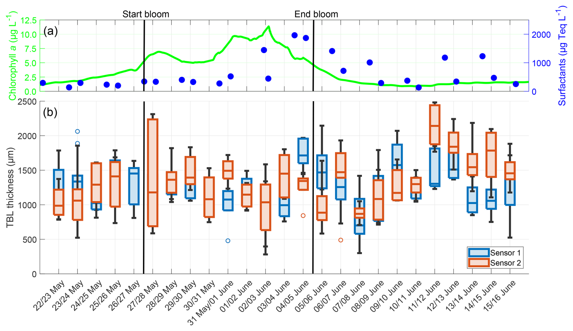
Figure 9 (a) ULW chlorophyll a concentration (green) and SML surfactant concentration (blue) between 22 May and 16 June, (b) TBL thickness from Sensor 1 (blue) and Sensor 2 (red) during the nights between 22 May and 16 June, 4–10 profiles per night, box: 25 % to 75 % quartile, horizontal line: median, whiskers: largest and smallest nonoutlier value, open circles: outliers (difference to next value >1.5 times interquartile range). The solid black lines indicate the start and end points of the bloom phase.

3.7 Horizontal temperature gradients

The IR camera image from the post-bloom phase on 11 June revealed a heterogenous temperature distribution, highlighting distinct horizontal temperature gradients across the field of view, which measured 1.061 m × 0.812 m (Fig. 10a). Zooming in, the two white lines show examples of strong gradients (Fig. 10b). The upper-left line indicates a temperature difference of 0.232 °C over a distance of 32.2 mm. The lower-right line indicates a temperature difference of 0.224 °C over a distance of 22.1 mm. Both examples illustrate the potential for substantial horizontal temperature variations within a small observed area of a few centimetres. While the IR camera only measured the temperature at the uppermost water surface (10–20 µm thickness) and not the temperature across the whole TBL, the water surface temperature still determined the shape of the microprofiles and thus the measured temperature differences across the TBL. The horizontal surface temperature differences support the observed temperature deviations measured by both temperature microsensors through this very local changing of the temperature microprofiles. On 11 June, the two microsensors, mounted a few centimetres apart, recorded a mean deviation in the temperature difference of 0.091 ± 0.099 °C, which falls well within the range of the horizontal temperature gradients detected by the IR camera.

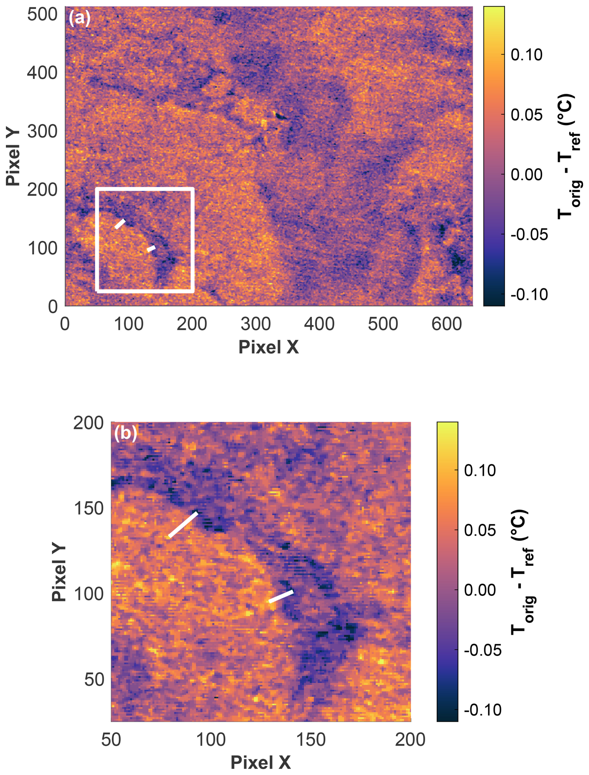
Figure 10 (a) Corrected IR camera image (T_orig − T_ref) from 11 June at 21:00:25 UTC (field of view = 1.061 m × 0.812 m, 100 pixels X = 0.166 m, 100 pixels Y = 0.159 m). The white square in (a) shows the zoomed view in (b): The two lines demonstrate two examples where, despite a small distance of 32.181 mm (top left) and 22.087 mm (bottom right), high temperature differences of 0.232 °C (top left) and 0.224 °C (bottom right) were measured.

4 Discussion

4.1 Measurements of the DBL and TBL

The use of microsensors and a microprofiling system provides a comprehensive dataset of in situ measurements of oxygen and temperature differences across the SML over several weeks in a mesocosm study. The high-resolution microprofiles have enabled the direct assessment of the DBL and TBL thicknesses. To investigate the effect of the phytoplankton bloom on these properties solely, night-time microprofiles were analysed. This excluded atmospheric influences, such as solar radiation and wind forcing at the water surface, and reduced the effect of diurnal warming to a minimum. Despite calm conditions without wind, the flow pumps generated light currents, which prevented a fully stagnant water column. Both oxygen and temperature microprofiles provide insights into the processes and properties of the SML, such as the thicknesses of diffusion and thermal boundary layers, oxygen and temperature differences across these layers, and gas exchange rates, which were typically measured indirectly in previous studies.

The study of air–sea gas exchanges has long been prevalent, from the proposal of a two-film model by Whitman (1962) to many other studies and concepts (Danckwerts, 1951; Liss and Slater, 1974; Deacon, 1977; Woolf, 1997; Asher et al., 2004; Zappa et al., 2007). Our in situ oxygen microprofiles, measured under non-turbulent conditions, reveal a three-layer structure at the air–sea interface: two millimetre-thick layers in the air and ULW with notable oxygen gradients in the air, and one sharp diffusion boundary layer right at the air–sea interface, which connects both. Observations of air flow by Buckley and Veron (2016) revealed layers of reduced turbulence directly above the water surface, which are prevalent under various atmospheric conditions. Our measurements indicate that significant gradients in oxygen partial pressure are present in these layers. Since gas flux measurements are often performed at heights of several metres above the water surface (Rutgersson et al., 2016; Wanninkhof et al., 2019), the presence of these millimetre-scale gradients near the surface leads to uncertainties in the parameterisation of surface gradients and gas fluxes.

Our measurements show that the DBL thickness (936.73 ± 369.49 µm) is significantly larger than the 50 µm thickness of diffusion sublayers defined by GESAMP (1995). It is, however, close to their definition of the viscous sublayer thickness, which is 1000 µm for a layer of reduced turbulence. Our measurements align well with the 1100 µm thick DBL, that Rahlff et al. (2019) measured using microsensors under laboratory conditions. However, they are significantly larger than the 350–500 µm reported by Adenaya et al. (2021), who applied a similar technique but did not include phytoplankton in their study. For other gases, whose fluxes are also predominantly dependent on properties of the water, like CO₂ (Liss, 1973; Ribas-Ribas et al., 2018), a DBL thickness of 50 µm is assumed (Robertson and Watson, 1992). Our measurements of the DBL indicate that its thickness under calm conditions is substantially underestimated and instead falls within the region of the viscous sublayer. While our study shows a case without turbulence, its findings are important to consider when calculating gas fluxes under calm conditions and underline the need for gas flux measurements as close as possible to the water surface.

Studies for determining the TBL thickness and temperature gradients often rely on indirect measurements and remote sensing of the surface temperature, using physical principles based on the temperature difference across the TBL and the sum of radiative heat fluxes (Saunders, 1967). While early studies deliver a wide range of TBL thickness estimates (Ginzburg et al., 1977), more recent studies often assume a TBL thickness of around 1 mm (Donlon et al., 2002; Jaeger et al., 2025). Our mean TBL thickness of 1299.5 ± 391.8 µm is consistent with these recent measurements, but significantly thicker than the 300 µm thick thermal surface layer reported by GESAMP (1995). It has been shown, that increasing wind speeds above 2 m s⁻¹ lead to a decrease in the TBL thickness (Ginzburg et al., 1977; Sromovsky et al., 1999; Murray et al., 2000; Wong and Minnett, 2018). As our measurements are conducted without wind, a slightly thicker TBL is expected than those reported in the literature. For example, Ward and Donelan (2006) implemented temperature microprofiles under changing wind speeds and air–water temperature differences. They measured a strong decrease in TBL thickness at increasing low wind speeds, from 2.16 mm at 1 m s⁻¹ to 0.55 mm at 3 m s⁻¹ for a warm TBL, and a 0.44 mm thick colder TBL with a wind speed of 4 m s⁻¹. While our TBL thickness is as expected higher than their thicknesses under increasing wind speeds, it is lower than their warm TBL thickness at the lowest wind speed. While Ward and Donelan used freshwater without surfactants and a different microprofile analysis method, their results indicate for our experiment not only a strong thinning of the TBL with the onset of low winds, but also differences between warm and cold TBL thicknesses at similar conditions.

A colder water surface compared to subsurface water, called “cool skin layer”, is commonly observed with temperature differences between −0.1 and −0.2 °C (Donlon et al., 1999; Murray et al., 2000; Donlon et al., 2002; Minnett et al., 2011; Jaeger et al., 2025). Our in situ measurements of the mean temperature difference of −0.133 ± 0.079 °C are consistent with these measurements. Most of these common observations, however, were made in field conditions, where wind enhances the cool skin effect. Our measurements indicate that a cool skin layer can also be present at night, consistently reaching a temperature difference comparable to field conditions due to net heat loss, even under mostly calm conditions. A temperature equilibrium between air and water was not achieved due to the continuing diurnal changes in air temperature which affected the water surface temperature even with a closed roof. Common parametrisations of the cool skin effect, solely based on wind speed, are often not defined for low wind regimes due to a lack of observational data (Donlon et al., 2002; Minnett et al., 2011). Other parameters influencing the net heat flux, such as buoyancy fluxes, water surface temperature or air temperature and humidity, must be additionally considered when calculating cool skin effects at very low wind speeds (Soloviev and Schüssel, 1994; Fairall et al., 2003; Minnett et al., 2011). The heterogeneous temperature distribution we detected with the IR camera under slick conditions, which also occurs under rain conditions (Wurl et al., 2019), highlights the need to base these calculations not only on measurements from a single point, but on the mean from a larger area. The extent, to which these distinct horizontal temperature distributions continue beyond the sea surface into the ULW remains unclear, as high-resolution thermal images are limited to the upper 10–20 µm of the water surface.

4.2 Influence of the phytoplankton bloom

The phytoplankton bloom has significantly different effects on the oxygen compared to the temperature. The increased daytime production of oxygen during the bloom resulted in approximately a 20 % increase in oxygen concentration in the ULW, which persisted into the night and was gradually depleted through respiratory processes. This led to increased oxygen differences across the DBL, and a strong correlation was observed with the chlorophyll a, which acted as a proxy for the bloom. The temperature differences, however, showed no correlation to the chlorophyll a, and thus no direct impact of the bloom. While such a direct impact of the bloom on the temperature was not expected, these results show that there was no indirect impact of the bloom on the water temperature, e.g., through surfactant production. We suggest that the temperature differences were limited by buoyancy fluxes, in which a decrease in surface temperature led to an increased density and a replacement of the surface water with less dense ULW (Soloviev and Schüssel, 1994). These buoyancy fluxes could not be resolved by the microprofiles, as they occur on scales of a few minutes (Wurl et al., 2019). They also impact the exchange of oxygen and other gases, as surface water, which becomes gradually depleted in oxygen due to diffusive fluxes with the atmosphere, is regularly replaced with more oxygen-rich underlying water (MacIntyre et al., 2002).

The thickness of the diffusion boundary layer is not directly related to the chlorophyll a and shows no correlation with the oxygen differences. It is, however, moderately correlated to the surfactant concentration. While the peak of the surfactant concentration is a result of the phytoplankton bloom, the higher levels during the post-bloom phase are a result of the subsequent bacterial bloom, as both are producers of surfactants (Žutić et al., 1981; Kurata et al., 2016). Surfactants are known to directly retain molecular exchanges between the ocean and atmosphere, leading to a thicker DBL and decreasing gas exchange (Liss, 1977; Cunliffe et al., 2013; Ribas-Ribas et al., 2018; Mustaffa et al., 2020). On the contrary, the TBL thickness showed no correlation with the surfactants but a moderate correlation with the temperature differences. This leads to the assumption that the direct effect of surfactants in reducing air–sea exchanges may be more effective for gas exchanges, such as oxygen exchange, but less effective for heat exchange. The SML with varying concentrations of surfactants significantly impedes oxygen transfer along concentration gradients (Goldman et al., 1988; Wurl et al., 2011; Rahlff et al., 2019). Heat, however, is exchanged much faster than oxygen, because the thermal diffusion coefficient in water is by two magnitudes greater than the oxygen diffusion coefficient (Bindhu et al., 1998; Ambari et al., 2022). Due to the faster heat exchanges, surfactants might be less effective in reducing air–sea heat exchanges than oxygen exchanges.

The natural surfactants produced during and after the bloom, lead to the formation of a slick, which altered the horizontal surface temperature distribution. Material floating on the slick-like water surface lead to very heterogenous surface temperatures. Our approach differs from laboratory studies that used artificial surfactants to generate slicks via monolayers. These studies showed that under calm conditions, slicks lead to more homogeneous surface temperatures (Saylor et al., 2000; Flack et al., 2001; Saylor et al., 2001). These different approaches lead to inconsistent results between laboratory and field studies, which mesocosm studies can close by bringing closer-to-field conditions into laboratory-like experiments.

The high gas exchange rate in the bloom and post-bloom phases shows the combined influence of both the phytoplankton bloom and the subsequent bacterial bloom, as both lead to a decrease in oxygen concentration during the night through heterotrophic processes. Furthermore, we observed a constantly positive gas exchange rate and a reduction in oxygen concentration throughout the night, even when the diffusive rate was negative, indicating a diffusive increase in oxygen concentration. This underlines that biological processes in the mesocosm, not diffusive fluxes with the atmosphere, drove the oxygen concentration. This is supported by Rahlff et al. (2019), who also demonstrate that biological factors significantly outweigh the diffusive processes in oxygen concentration. They further demonstrate that biological processes in the ULW, rather than in the SML, drive the oxygen concentration at the water surface. In this study, chlorophyll a and phytoplankton abundance were only measured in the ULW but not the SML. The findings of Rahlff et al. (2019) provide confidence that no significant influence of biological processes within the SML was overlooked and that the processes measured in the ULW substantially control those in the SML.

4.3 Perspective: DBL and TBL under oceanic conditions

While the influence of wind was excluded in the analysis to focus on the impact of the phytoplankton bloom, it is essential to note that wind would have a significant effect on the DBL and TBL, leading to near-surface turbulent mixing (Liss, 1973; Ginzburg et al., 1977; Donlon et al., 1999; Murray et al., 2000; MacIntyre et al., 2002). These turbulent conditions may lead to enhanced exchanges between the SML, ULW, and atmosphere, resulting in smaller surface gradients and thinner, less distinct surface layers (Sromovsky et al., 1999; Wurl et al., 2011). Surfactants have both a direct effect on air–sea exchanges by retaining molecular exchanges at the surface and an indirect effect by reducing turbulence and damping waves (Liss, 1977; Goldman et al., 1988; Laxague et al., 2024). While this study shows the direct effects of surfactants retaining exchanges across the water surface, the presence of wind would enhance the indirect effects on gas and heat exchanges. Thus, the bloom's impact on surface properties might be disproportionally high under higher wind conditions, as it increases surfactant production and reduces the wind-driven turbulence.

Although the microsensor measurements were only taken at one point inside the mesocosm, the slow movement of the water ensured that a larger water mass was measured, making the measurements representative of the entire mesocosm. At each vertical step, measurements were integrated over a 30 s period, and a complete profile required 40–50 min to record. Consequently, the profiles reflect mean conditions during this interval rather than instantaneous values, and fast surface processes, such as buoyancy fluxes, could not be resolved. While wind would make microsensor measurements more field-realistic, the resulting waves introduced high variability into the profiles. This variability was especially pronounced near the surface, making it challenging to accurately determine differences and boundary layer thicknesses.

The strong influence of phytoplankton blooms may have global implications, as slicks, often formed by these blooms, cover large parts of the oceans and have significant impacts on air–sea gas exchange (Goldman et al., 1988; Romano, 1996; Mustaffa et al., 2020). The effect of these blooms on the SML temperature, while not pronounced under no-wind conditions, is potentially relevant for global heat exchanges under typical oceanic wind conditions. Wurl et al. (2018) have already shown that natural slicks can have a significant impact on the temperature and salinity of the SML, indicating retention of evaporation. This mesocosm study further shows the need to expand cool skin parametrisations to low wind conditions. Uncertainties in these parametrisations can have considerable implications, from validating satellite sea surface temperature measurements (Cronin et al., 2019), to having an impact on gas fluxes with the atmosphere (Ward et al., 2004; Yang and Langdon, 2025) and the calculation of air–sea heat and freshwater fluxes, impacting the weather and climate (Grist et al., 2016; Zhao and Knutson, 2024).

While the use of microsensors under conditions with wind proved difficult, more in situ data of the DBL and TBL under varying wind conditions are needed, not only to assess the wind influence on the microprofiles, but also to investigate the indirect effects of surfactants on gas and heat exchanges through their turbulence-reducing properties. The use of microsensors in our mesocosm study enabled us to gain a mechanistic understanding of how phytoplankton blooms affect the DBL and TBL. Our in situ measurements provide direct insights into the oxygen and temperature across the SML. These results represent a significant step in highlighting the importance of the SML for large-scale air–sea exchanges, based on in situ observations.

5 Conclusion

The mesocosm study, as part of an interdisciplinary study, provides high-resolution in situ measurements of oxygen concentration and temperature across the SML. Microsensors were used to obtain continuous in situ microprofiles from the air, through the SML, into the ULW, which were utilised to calculate surface differences of oxygen and temperature, as well as the thicknesses of the oxygen diffusion boundary layer and thermal boundary layer. These in situ measurements revealed a strong correlation between the oxygen differences and chlorophyll a concentration, while the DBL thickness was moderately correlated with surfactant concentration. The blooms of phytoplankton and bacteria, through oxygen production, consumption, and surfactant production, heavily influenced the DBL. On the temperature differences and TBL thickness, the phytoplankton bloom had no direct effect under wind-free conditions. With the inclusion of wind, the impact of surfactants on the DBL and TBL would likely increase, and the phytoplankton bloom would have an even greater impact on the SML properties. Overall, the microprofiles obtained by the microsensors proved valuable for gathering in situ data on previously scarcely measured properties of the SML, while simultaneously assessing the effect of the phytoplankton bloom on these properties.

Appendix A: Comparison of oxygen microsensors with different calibrations

In May 2024, a separate experiment was conducted inside SURF, where one daily-calibrated and temperature-corrected oxygen microsensor and one oxygen microsensor, which was only calibrated at the start of the experiment and not temperature-corrected, were compared. Both were mounted close to the inlet of a FerryBox (-4H-Jena PocketBox, 4H Jena Engineering, Germany) at approximately 30 cm water depth. The FerryBox measured the oxygen concentration (corrected with discrete samples analysed with the Winkler method) and water temperature. The microsensor data were filtered for clarity, using a Hampel filter, replacing outliers within a 10 min window that differed from the median by more than three standard deviations with the median value. The results showed that daily calibration sometimes led to large jumps in oxygen concentration, depending on the temperature at the time of calibration (Fig. A1). No consistent offset was established between the daily calibrated sensor and the once-calibrated sensor. The offset of both microsensors compared to the FerryBox was similar. This experiment demonstrated that the lack of daily calibration likely did not lead to large offsets in the oxygen microsensor measurements obtained during the mesocosm experiment.

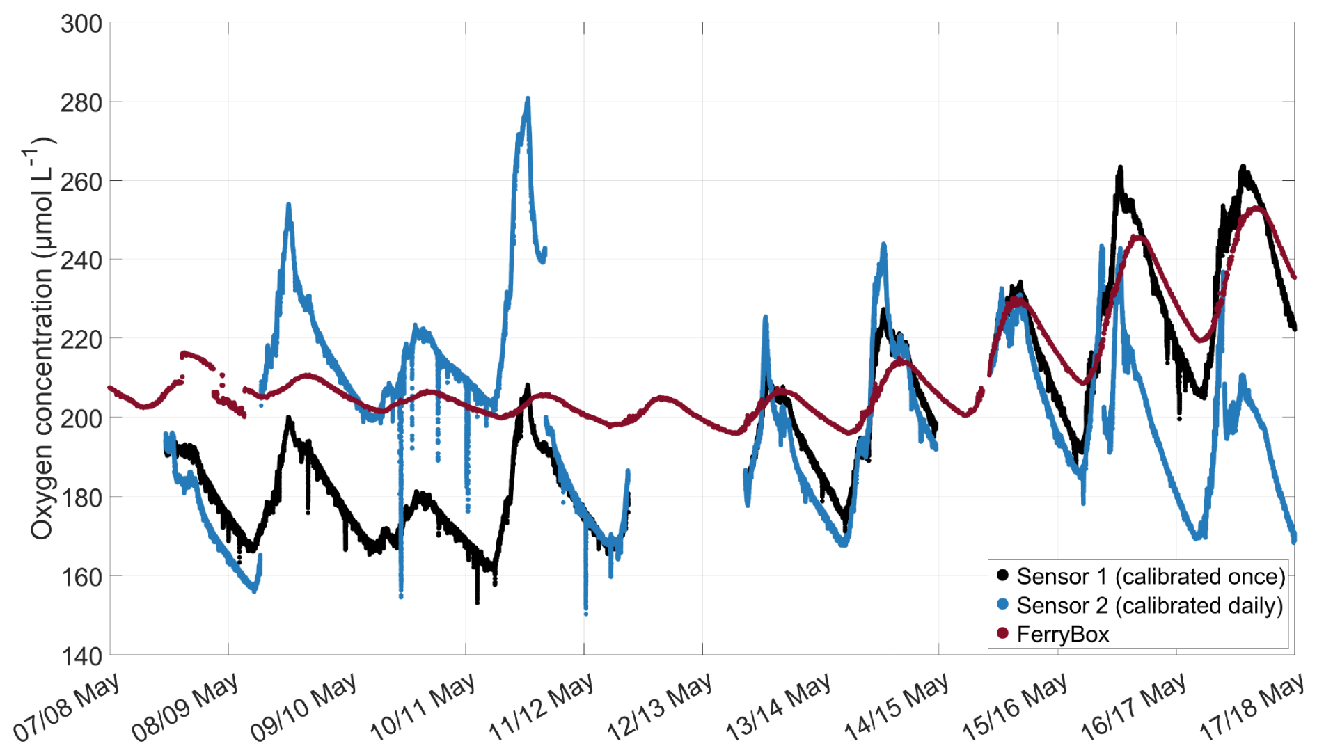
Figure A1 Comparison of the oxygen concentration measured by an oxygen microsensor calibrated at the start of the experiment and not corrected for temperature (black), one microsensor calibrated daily and corrected for temperature (blue), and corrected oxygen concentration measured by a FerryBox (red), experiment conducted in May 2024 in SURF. Microsensor data are filtered using a Hampel filter with a 10 min window.

Appendix B: Comparison of the oxygen microsensor with the FerryBox

The oxygen concentration measured by the microsensor during the main mesocosm study was compared with oxygen measurements from a FerryBox (-4H-Jena PocketBox, 4H Jena Engineering, Germany), which were corrected using discrete samples analysed with the Winkler method. These discrete samples were taken daily at alternating times (one day early morning, the next day afternoon) to account for diurnal changes in oxygen concentration. The inlet of the FerryBox was located at approximately 40 cm depth. The comparison of the mean microsensor measurements from the ULW (ranging approximately between 1 and 7 mm) and FerryBox shows that both measurements were typically consistent, but with a time lag that could reach more than three hours (Fig. B1). Only in the post-bloom phase was a larger offset observed, as indicated by higher oxygen concentrations measured by the microsensors. These offsets can be attributed to a growing oxygen gradient in the ULW between the microsensors and the FerryBox, which can also be seen in the microsensor profiles during this time (Fig. 4c). The results provide more confidence in the quality of the oxygen microsensor data, even if the microsensor was only calibrated once and not corrected for temperature.

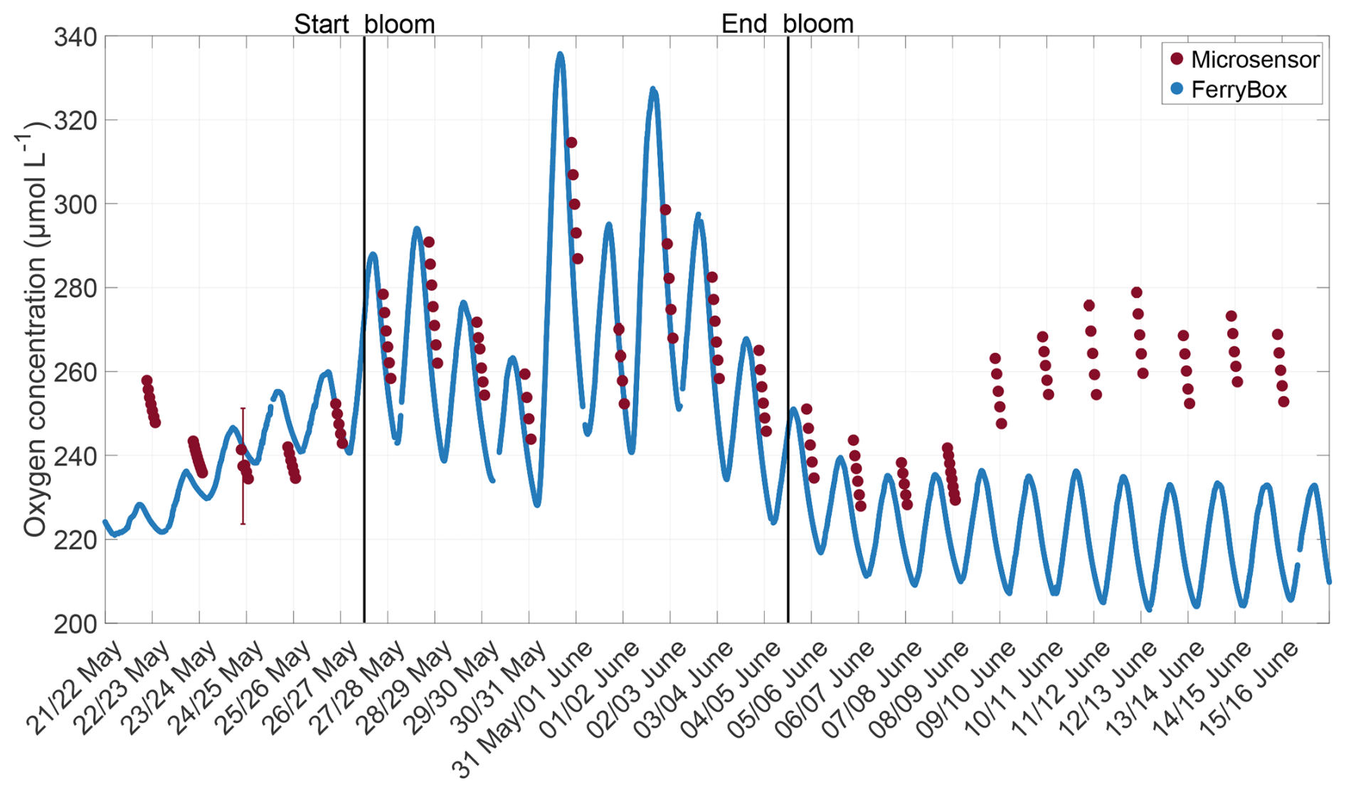
Figure B1 Corrected oxygen concentration measured by the FerryBox at 40 cm depth (blue) and by the oxygen microsensor (red), mean from the lower end of the DBL to the end of the profile. The solid black lines indicate the start and end points of the bloom phase.

Appendix C: Oxygen saturation

The microsensor profiles were used to compute the oxygen saturation of the surface water. The oxygen concentration and temperature measured by the microsensors below H₀, along with the salinity of the CTD at a depth of 40 cm, were used to calculate the oxygen saturation profiles of the water using the Gibbs-Sea Water (GSW) Oceanographic Toolbox for MATLAB (McDougall and Barker, 2011). Differences compared to the calculation using salinity data from the CTD near the surface, which had a poorer data quality due to many outliers, were approximately 0.14 % and not statistically significant.

The oxygen saturation trend was very similar to the trend in gas exchange rates (Fig. C1). It had a minimum of 96 % in the pre-bloom phase, then increased during the bloom phase to 127 %, and decreased in the early post-bloom phase to 101 %. Contrary to the trend in oxygen differences, but similar to the trend in gas exchange rates, oxygen saturation increased again in the post-bloom phase to approximately 120 %. This also coincided with the post-bloom increase in bacterial abundance. The increased post-bloom oxygen saturation can be attributed to the formation of biofilms on the floor, walls, and submerged equipment of SURF. These biofilms have been shown to contain cyanobacteria, which contribute to increased oxygen production (Kühl et al., 1996; Pringault and Garcia-Pichel, 2000). The mean oxygen saturation over the entire study was 109.37 ± 9.00 %. Pre-bloom, it was 99.80 ± 3.88 %, rose during the bloom phase to 111.89 ± 6.64 %, and subsequently increased slightly to 112.35 ± 8.94 % in the post-bloom phase. Rising water temperatures during the mesocosm study (approximately a 7 °C increase from 18 May to 16 June; Bibi et al., 2025a) only partly explain this increase, as oxygen saturations were still 10 % higher post-bloom compared to pre-bloom when calculated with a constant temperature.

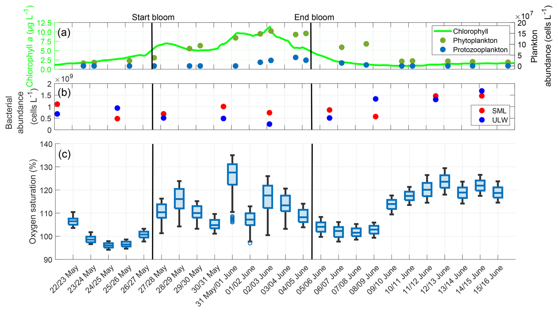
Figure C1 (a) ULW chlorophyll a concentration (green), phytoplankton abundance (dark-green) and protozooplankton abundance (blue) between 22 May and 16 June, (b) Bacterial abundance in the SML (red) and ULW (blue), (c) Oxygen saturation during the nights, boxplots show all the oxygen saturation data in the DBL and ULW, box: 25 % to 75 % quartile, horizontal line: median, whiskers: largest and smallest value, open circles: outliers (difference to next value >1.5 times interquartile range). The solid black lines indicate the start and end points of the bloom phase.

Appendix D: Oxygen diffusive rates

In addition to the single gas exchange rate per night, the vertical diffusive rate for each profile during the night was calculated using Eq. (D1) as described by Rahlff et al. (2019). It illustrates the vertical oxygen loss from water to air through diffusive processes in the absence of wind, while the gas exchange rate refers to the total rate of change in oxygen concentration during each night, regardless of driving factors.

$$\begin{array}{}\text{(D1)}& \mathrm{DR}=D\cdot {\displaystyle \frac{A}{V}}\cdot {\displaystyle \frac{\mathrm{1}}{\mathit{\delta }}}\cdot (C_{\mathrm{HDBL}}-C_{H_{\mathrm{0}}}),\end{array}$$

DR [µmol L⁻¹ h⁻¹] is the vertical diffusive rate, and D [cm h⁻¹] is the diffusion coefficient dependent on the temperature and salinity, which was obtained from the table of Ramsing and Gundersen (2000) using the microsensor temperature at H_TBL and the salinity measured by the CTD in the ULW. V [cm³] is the water volume and A [cm²] the water surface area of SURF, δ [cm] is the DBL thickness, and $C_{\mathrm{HDBL}}-C_{H_{\mathrm{0}}}$ [µmol L⁻¹] is the oxygen difference in the DBL. Compared with Rahlff et al. (2019), the direction of the diffusive rate was adjusted to align with the definition of the oxygen difference direction in this study. If the diffusive rate was positive, oxygen diffused from the water into the air, and vice versa.

The diffusive rates of oxygen were strongly correlated with the chlorophyll a concentration (r=0.745, p<0.001), but not with the surfactant concentration (r=0.239, p=0.250) (Fig. D1). With a 3 d lag, the correlation between the diffusive rate and surfactant concentration increased to a moderate and significant level (r=0.668, p<0.001). The mean diffusive rate was +0.098 ± 0.225 µmol L⁻¹ h⁻¹, and there was a large increase during the bloom phase (+0.323 ± 0.243 µmol L⁻¹ h⁻¹) compared to the pre-bloom phase (−0.037 ± 0.081 µmol L⁻¹ h⁻¹) or post-bloom phase (−0.016 ± 0.060 µmol L⁻¹ h⁻¹). The trend in diffusive rates is very similar to the trend in oxygen differences, since the oxygen differences are a major factor in calculating the diffusive rates. The diffusive rates show that in the bloom phase, oxygen mostly diffused from the water into the air (positive rate), while it mostly diffused from the air into the water in the pre-bloom and post-bloom phases (negative rate).

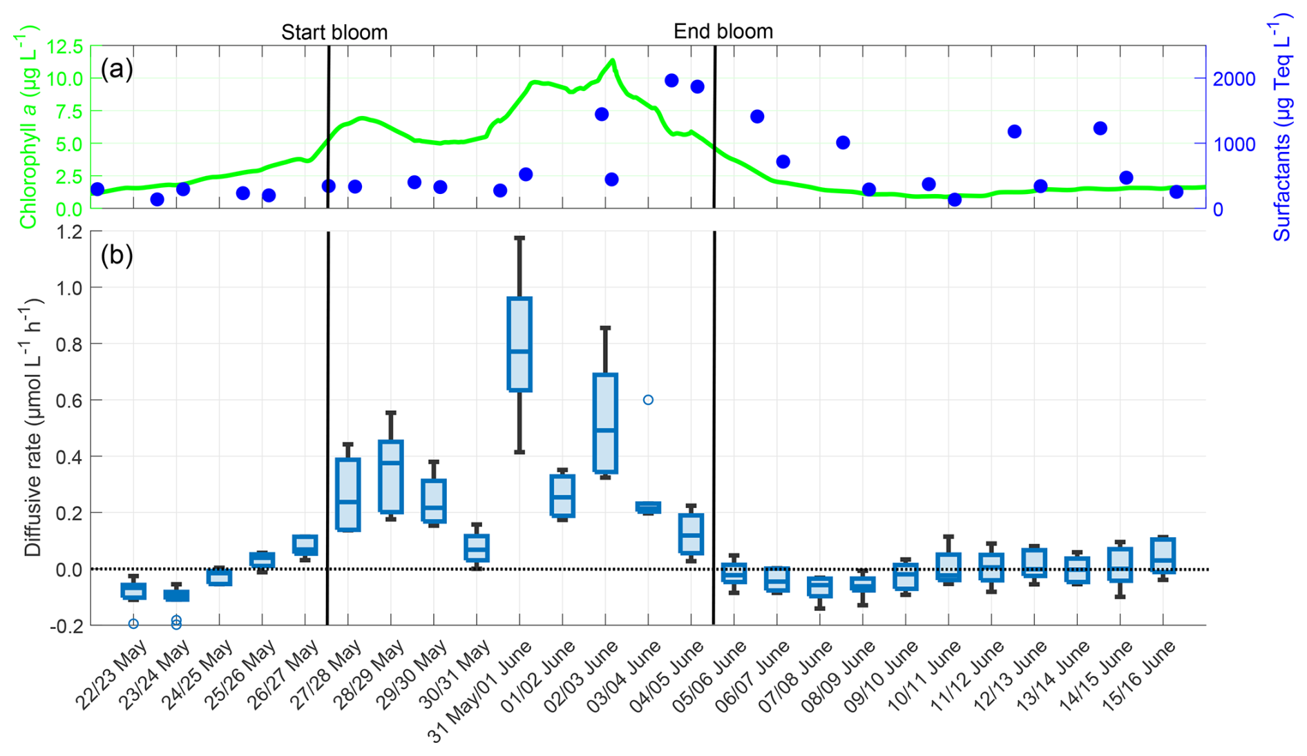
Figure D1 (a) ULW chlorophyll a concentration (green) and SML surfactant concentration (blue) between 22 May and 16 June, (b) Oxygen diffusive rate in the SML during the nights between 22 May and 16 June, 4–10 profiles per night, box: 25 % to 75 % quartile, horizontal line: median, whiskers: largest and smallest value, open circles: outliers (difference to next value >1.5 times interquartile range). The dotted line indicates the zero level and the solid black lines indicate the start and end points of the bloom phase.

Appendix E: Temperature microprofiles during one night

The temperature microprofiles on 22 May give a typical example of the profiles from both temperature sensors during all nights (Fig. E1). The warmest profile was the first of the night, and all the subsequent profiles were approximately 0.02 to 0.05 °C cooler than the preceding profile. The air temperature decreased as it moved farther from the water surface; it also decreased from profile to profile during the night and it was always lower than the water temperature. A cooler thermal boundary layer was present in all profiles. Sensor 2 measured up to 0.1 °C higher temperatures and was mounted approximately 750 µm deeper than Sensor 1. These slight deviations in mounting height and measured temperature were also observed on other nights, while the overall shape of the profiles remained very similar between both sensors. The only significant differences between nights for each sensor were the mounting height and the absolute temperature, which typically rose from night to night, starting at approximately 18.9 °C on 22 May and reaching around 22.6 °C on 15 June.

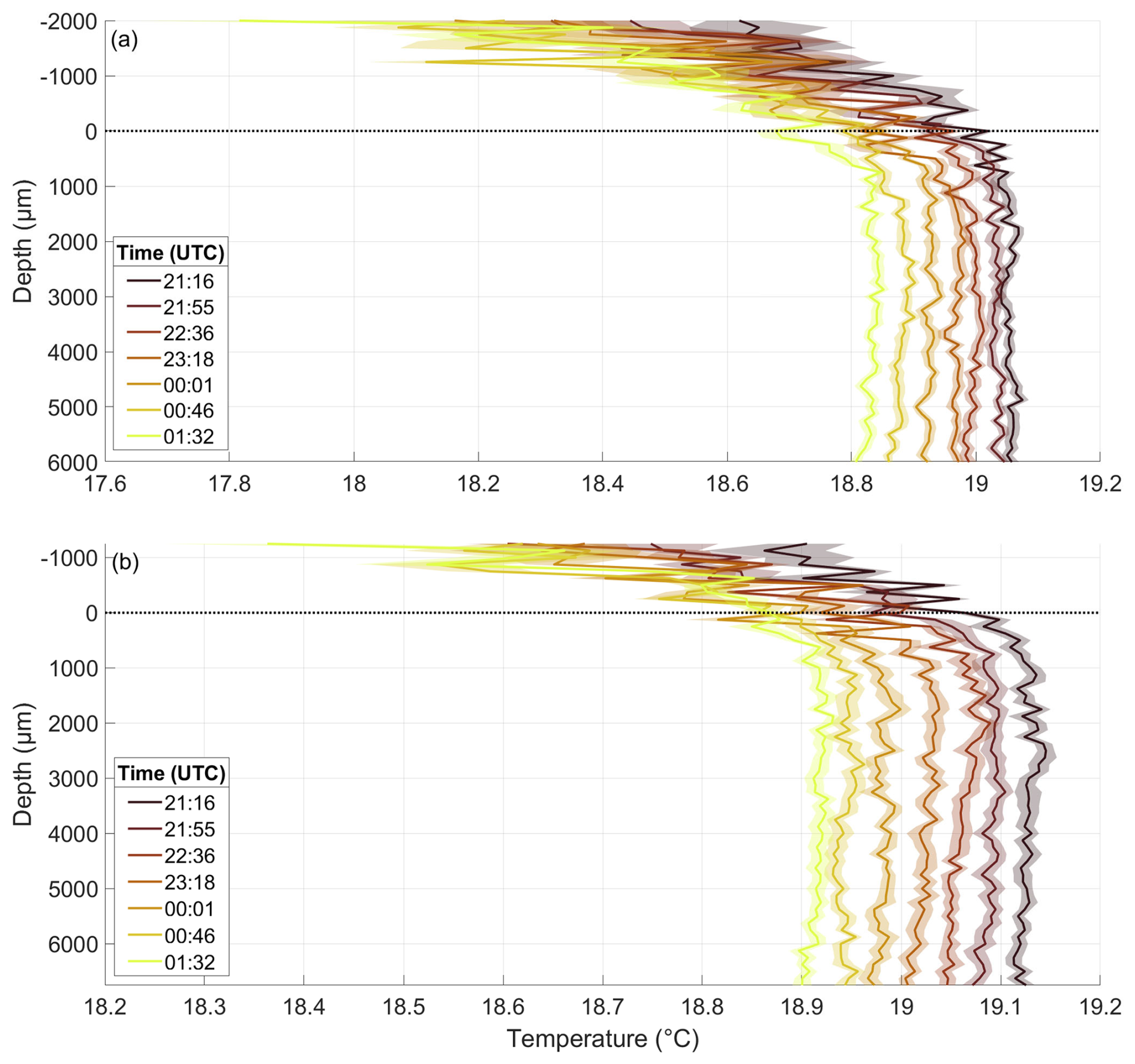
Figure E1 Temperature microprofiles of Sensor 1 (a) and Sensor 2 (b) throughout the night of 22 May, in the pre-bloom phase, depth corrected for the proper sensor position. 0 µm indicates the air–water interface (dotted line). Times are the mean times of the profile; one profile takes approximately 40 min to complete.