
the Creative Commons Attribution 4.0 License.
the Creative Commons Attribution 4.0 License.
 | 17 Nov 2026
Simulated Antarctic iceberg melting occurs primarily within the Southern Ocean mixed layer
Anna Olivé Abelló

Pierre Mathiot
Nicolas C. Jourdain
Yavor Kostov
Paul R. Holland
Although iceberg meltwater accounts for nearly half of the freshwater release from the Antarctic ice sheet, most ocean models do not represent the vertical distribution of this meltwater in a realistic way. Here, we investigate the importance of distributing the iceberg meltwater vertically in an ocean model that represents icebergs as Lagrangian particles. For more robust estimates, we update the iceberg melting laws: (i) we extend the three-equation formulation used for ice shelf melting to the iceberg basal melt parameterisation, (ii) we adopt a new formulation of lateral iceberg melt in which the buoyant plumes are fed by basal melt, and (iii) we improve the physical consistency of wave-induced ablation in our equations. The updated formulations produce a substantial increase in average lateral melt and a slight reduction in wave-induced ablation and basal melt compared to the pre-existing configuration. Seasonally, lateral melting becomes a major summer contributor, exceeding basal melting in magnitude, and all iceberg melting components decrease in winter. The enhanced sensitivity of wave-induced ablation to sea-ice concentration suppresses iceberg melting near the Antarctic margin, promoting longer iceberg lifetimes. Sensitivity simulations show that even when meltwater is evenly distributed in the vertical down to the iceberg keel depth, 76 %–87 % of the iceberg meltwater remains injected into the surface mixed layer. Freshwater injection at depth promotes warming and salinification of the Amundsen Sea near the seabed, and freshens and cools the East Antarctic and western Ross Sea continental shelves, but all these changes have a small magnitude. Also, it leads to thinner sea ice and locally enhanced sea-ice production, especially in the southwestern Weddell Sea. Overall, these results imply that for Southern Ocean-scale responses, modelling studies to date that release iceberg meltwater at the surface can still be considered reliable.
- Article
(13911 KB) - Full-text XML
-
Supplement
(33414 KB) - BibTeX
- EndNote


Antarctic icebergs account for nearly half of the ice-sheet mass loss in Antarctica (Depoorter et al., 2013). As they drift across the Southern Ocean under the influence of ocean currents and winds (Kostov et al., 2026), their melting is typically represented in ocean models as generating a shallow, low-salinity layer at the ocean surface. In these models, melting consumes latent heat and increases the ocean freezing temperature, which promotes sea-ice formation (Savage, 2001; Jongma et al., 2009; Merino et al., 2016; Ackermann et al., 2024). However, most of them still do not represent the vertical distribution of iceberg melting, which is a key limitation given that meltwater released at depth can either stabilise or destabilise the water column (e.g. Jourdain et al., 2017; FitzMaurice et al., 2017). While surface melting enhances the ocean stratification, subsurface discharge can instead generate buoyant plumes and vertical mixing, which can induce the upward entrainment of relatively warm and salty Circumpolar Deep Water (CDW) toward the surface (Silva et al., 2006; Jenkins, 1999).
Only a few direct observations exist near individual icebergs. Close to the giant iceberg C18a, Helly et al. (2011) measured surface freshening and cooling extended down to depths of 50–90 m, persisting in a reduced form after 10 d. Similarly, Wagner et al. (2018) reported the presence of a cold surface layer around 25 m thick, with a decline of 0.8 in salinity and 3 °C in temperature within 10 km of the presence of small icebergs. Building on previous studies, recent observations from Lucas et al. (2025) revealed that, near the giant iceberg A68a, the strongest water-column impacts were confined to the upper 20 m, as well as around and below the iceberg draft depth, but could not be detected more than 5 km away from its edge. However, the large-scale significance of meltwater released at different depths from observed giant icebergs remains unknown, with some iceberg thicknesses exceeding 650 m (Olivé Abelló et al., 2025; Dowdeswell and Bamber, 2007) and releasing around 668 Gt yr−1 south of 63° S from ocean model estimates (Silva et al., 2006).
In most of these ocean–iceberg models used for large-scale oceanographic and climatological studies, iceberg melting usually consists of three components: basal melting, wave-induced ablation, and lateral melting by buoyant convection. Iceberg surface melting, such as that driven by solar radiation and sensible heating, is usually considered negligible compared to these three processes (e.g. Bigg et al., 1997; Gladstone et al., 2001; Martin and Adcroft, 2010). Basal melting is driven by turbulent heat transfer from the ocean below and is enhanced by strong ocean–iceberg relative velocity (Bigg et al., 1997; Martin and Adcroft, 2010). Lateral melting along the submerged sidewalls occurs through a similar process, but is instead driven by buoyant convection. Wave-induced ablation results from enhanced melting near the ocean surface, where the warm surface layer and the strong turbulence generated by wind-driven wave breaking increase heat transfer at the iceberg sidewall and promote notch formation at the waterline (Savage, 2001; El-Tahan et al., 1987). As these notches deepen, the ice slabs above and below become destabilised and eventually collapse (White et al., 1980; Sartore et al., 2025; Scambos et al., 2005; Wagner et al., 2014). The depth at which models should inject the meltwater originating from each of these three melting components remains an open question.
Laboratory experiments indicate that releasing all the basal and lateral meltwater at the surface is only appropriate when the relative velocity between the iceberg and the surrounding ocean is smaller than the vertical velocity of the meltwater plume (FitzMaurice et al., 2017). For stronger ocean–iceberg relative velocities, the meltwater plume no longer rises uniformly; instead, the freshwater mixes laterally with the ambient water before reaching the surface. Similarly, the depth at which to inject meltwater from wave-induced ablation also remains uncertain. Wave-induced ablation itself occurs at the waterline, and the subsequent collapsed ice slabs end up as small bergy bits melting near the ocean surface, but the vertical ocean mixing occurring during the collapse may further redistribute meltwater within the upper ocean (consistent with observations from ice-mélange collapse in Greenland fjords, where induced changes in the water column extend to depths of 200 m as described by Abib et al., 2024).
Recently, some studies have started to spread the iceberg meltwater flux vertically over the upper 350 m of the water column using the MITgcm ocean model (Naughten et al., 2022; Moorman et al., 2026), without producing excessive stratification. In parallel, Amaral Wasielesky (2025) has made the first attempt in the NEMO ocean model (Nucleus for European Modelling of the Ocean; Madec and the NEMO System Team, 2022) to release the total iceberg melt at two different depths (at the surface vs. vertically distributed down to the iceberg keel depth) for icebergs calved from the Greenland Ice Sheet. They found that, in regions densely populated with icebergs, meltwater released at depth enhanced vertical mixing, which in turn increased melt rates, facilitated the downward dispersion of freshwater, and entrained warmer and saltier waters into the upper subpolar North Atlantic. In Antarctica, icebergs can be significantly thicker than in Greenland (Olivé Abelló et al., 2025), which raises the question of which depth is appropriate to release all the Antarctic iceberg meltwater and how releasing it at depth will alter the Southern Ocean response.
These advances highlight the need to revise the vertical distribution of iceberg melt across different depths. Because of that, the main aim of this study is to assess different combinations of basal melting, wave-induced ablation, and lateral melting processes to move towards a more realistic representation of the vertical injection of iceberg melting (Sect. 2). Then, we analyse the temporal and spatial differences in freshwater magnitude, as well as the impacts of the updated melting parameterisations at depth on sea-ice thickness, concentration, and production, water-column and bottom temperatures and salinities, and ice-shelf melting (Sect. 3). Finally, we discuss the limitations, the consistency of our results with the existing literature, and the local rapid dilution of iceberg meltwater in the ocean in Sect. 4, and conclude in Sect. 5.
2.1 Ocean–iceberg model
We use the NEMO 4.2 ocean–sea-ice model (Madec and the NEMO System Team, 2022) in a circumantarctic configuration eANT025.L121, where the northern domain boundary reaches 52.25° S (Mathiot and Jourdain, 2023). The model has a horizontal resolution of 0.25° and 121 vertical levels, forced by a repeated normal year of JRA55-do atmospheric data (1990–1991; Kobayashi et al., 2015). A constant calving flux is prescribed following Rignot et al. (2013), assuming a steady-state calving front, with the flux randomly distributed across the ocean grid cells along the ice-shelf front.
In the following sensitivity experiments (see Sect. 2.3), we consider 10 iceberg size classes, a maximum iceberg area of 4 km2, and a maximum calving iceberg thickness prescribed from the ice-shelf thickness at the nearest calving front, based on the BedMachine-v3 dataset (Morlighem, 2022; Morlighem et al., 2020), following Olivé Abelló et al. (2025). Additionally, we incorporate a simple iceberg grounding scheme, and to optimise computational cost, we use a clustering R=2, in which a single Lagrangian particle representing a small iceberg class is representative of multiple icebergs of the same characteristics (Olivé Abelló et al., 2025). The forcing and setup details follow Mathiot and Jourdain (2023), except for the omission of the sea surface salinity restoring.

Figure 1Comparison of water-column properties at 500 m depth between the model simulation under the same conditions as in Olivé Abelló et al. (2025), hereafter PRE (see Sect. 2.3), and the World Ocean Atlas 2023 (WOA23) climatology (2015–2022). (a–c) Potential temperature (°C), (d–f) salinity, and (g–i) potential density (σ0, kg m−3). Black contours indicate (a, b) the 0 °C isotherm, (d, e) the 34.8 salinity isoline, and (g, h) the 27.7 kg m−3 isopycnal, typically used to identify the presence of CDW. In the difference panels (c, f, i), black contours indicate differences at 0.5 °C intervals for potential temperature and 0.1 intervals for salinity and potential density, with the zero contour highlighted by a thicker black line.
To assess whether the baseline model configuration is able to reproduce the observed ocean state before being used in our experiments, we compare the simulated water-column properties at 500 m depth with the World Ocean Atlas 2023 (WOA23) climatology (2015–2022; Fig. 1). Despite regional biases, the model broadly reproduces the observed large-scale upper-ocean potential temperature, practical salinity, and potential density patterns of the Southern Ocean at this depth, with slightly saltier and hence denser waters (Fig. 1f and i) around the Antarctic continent. Over the continental shelf, some of the largest temperature and salinity discrepancies occur, especially in the eastern Ross Sea, at the tip of the Antarctic Peninsula, and locally in East Antarctica, although these are usually largely compensated in terms of potential density, with differences rarely exceeding 0.2 kg m−3. In terms of water-mass distribution, the model captures the main large-scale features associated with relatively warm modified Circumpolar Deep Water (mCDW; usually characterized by θ>0 °C and salinity>34.8) in the Amundsen and Bellingshausen Seas, although WOA23 seems to underestimate its temperature and salinity on the eastern Amundsen Sea continental shelf (Fig. 1b and e). In East Antarctica, WOA23 shows mCDW intrusions onto the continental shelf reaching several ice shelves, including Totten, Rennick, Moscow University, and Denman (e.g. Rintoul et al., 2025, 2016), whereas in the model the continental shelf remains cold, with temperatures below −0.2 °C in these regions. These warm-water intrusions are relevant as they may enhance iceberg melting by providing heat along the submerged iceberg keel. Further information on the model configuration and the experimental design bases is provided in Olivé Abelló et al. (2025).
2.2 Alternative iceberg melt formulation
Most classical iceberg melting formulations in numerical ocean models remain simple and largely empirical, with parameters constrained by a limited number of cruise observations (Bigg et al., 1997; Gladstone et al., 2001). Several studies have opted to incorporate more physically based alternatives, as the validity of these empirical formulations has been increasingly questioned (Hester et al., 2021; Sartore et al., 2025). For instance, the bulk basal melting parameterisation defined by Weeks and Campbell (1973) has been replaced in some models that include dynamical icebergs (Rackow et al., 2017) by the more physically constrained three-equation formulation of Holland and Jenkins (1999), which produces more realistic iceberg meltwater fields in the Southern Ocean, particularly for giant icebergs (Silva et al., 2006). The iceberg aspect ratio (length-to-draft) also exerts a strong influence on the relative importance of side melt compared to basal melt rates, with large and thin tabular icebergs losing a greater fraction of their mass through basal melting than those with smaller aspect ratios (Cenedese and Straneo, 2023). Additionally, Hester et al. (2021) further emphasised the role of face orientation relative to the ambient flow, with melt rates per unit of area being highest on the forward-facing side, followed by the remaining lateral sides, and lowest at the base (although the overall melt rate will depend on iceberg aspect ratio). In this context, we therefore propose an alternative set of parameterisations based on recent studies and physical considerations.
The pre-existing bulk formulation of the basal melt rate Mb in NEMO is an empirical dependency on the ocean–iceberg velocity and ocean temperature (Weeks and Campbell, 1973; Savage, 2001; Martin and Adcroft, 2010). Here, we adopt the so-called three-equation formulation for Mb, which is a standard way to parameterise ice-shelf basal melting, accounting for heat and salt budgets at the ice–ocean interface and for the salt and depth dependency of the freezing temperature (Holland and Jenkins, 1999; Jenkins et al., 2010). Equation (1) makes use of the formulation proposed by Asay-Davis et al. (2016), while neglecting ice thermal conduction, which is usually of secondary importance (Wiskandt and Jourdain, 2025):
where ρsw is the seawater density, Mb is the melt rate expressed in , L is the latent heat of fusion, cw is the specific heat capacity of seawater, and u* is the friction velocity, calculated as with cd the drag coefficient, (ui−uo)b the relative iceberg–ocean velocity at the ice base, and assuming a constant background velocity of ubkg=0.01 m s−1. ubkg represents the velocity of unresolved processes in our ocean model, such as Stokes drift, internal waves, Langmuir circulations, and other subgrid-scale motions that can enhance turbulent mixing at the iceberg base and thus increase its friction velocity. ΓT and ΓS are the NEMO non-dimensional heat and salt turbulent transfer coefficients as in Asay-Davis et al. (2016), and Tw and Sw are the ocean potential temperature and salinity at the depth of the iceberg base. This alternative parameterisation, unlike the one pre-existing in NEMO, takes into account the freezing point (Tz) dependency on pressure and salinity through the λ1, λ2, and λ3 coefficients.
Regarding the lateral melt rate Mv, the pre-existing formulation implemented in NEMO is a second-order polynomial in ocean temperature, empirically proposed by El-Tahan et al. (1987) for icebergs in the Arctic. Such a formulation lacks a salinity dependency, and its validity for large temperature ranges can be questioned (Jourdain et al., 2022, their Supplement). One alternative would also be to apply the three-equation formulation along the vertical iceberg sidewalls. However, since the three-equation formulation is fundamentally a shear-driven turbulent boundary-layer parameterisation, it should not be used in models whose horizontal resolution remains too coarse (tens of kilometres) to resolve the rising meltwater flow and hence, characterise the boundary layer along the iceberg lateral face, promoting large melt biases (e.g. Weiss et al., 2025). Moreover, the physical assumptions underlying the three-equation formulation are not consistent with the processes controlling heat transfer along vertical ice faces, where mixing is primarily driven by eddies, internal waves, and buoyant meltwater plumes rather than by the melt-driven flow itself. Furthermore, iceberg basal melting should contribute to the initiation and strengthening of vertical plumes developing along the iceberg sidewalls. We therefore chose to use the formulation of Slater et al. (2020), which was developed and calibrated for melting at the front of Greenland tidewater glaciers. This parameterisation accounts for the buoyant subglacial runoff normalised by calving front area, assuming that the circulation at the foot of the glacier front is solely driven by buoyancy forcing associated with subglacial discharge (Rignot et al., 2016). In freely drifting icebergs, the buoyant meltwater plume also depends on the relative velocity driving the iceberg–ocean boundary layer, a parameter already included in our updated basal melt formulation. In our adaptation, the iceberg basal melt is normalised by the basal area of the iceberg and distributed over two of the lateral faces as , where D is the iceberg draft, 0.5 accounts for the partitioning of basal melt between the two lateral faces (assuming that plumes only develop on the sides opposing ocean currents as observed in e.g. FitzMaurice and Stern, 2018 and Hester et al., 2021), the coefficient cday=86 400 is introduced to ensure that the units are expressed in m d−1 and X denotes either the iceberg length, L, or width, W, depending on the orientation of the lateral face considered. As in Slater et al. (2020), the thermal forcing value, TF, has been obtained from the difference of ocean temperature and freezing temperature profiles and then averaged from the iceberg keel depth to the ocean surface. Hence, the revised lateral melt rate Mv (in ) is expressed as:
for each of the two lateral faces. The inclusion of ρfw (freshwater density) ensures dimensional consistency, while the +0.15 prevents from being zero in the absence of basal melt (Rignot et al., 2016), although in our implementation melt rates are set to zero for TF<0, preventing non-real values under supercooling conditions.
Finally, for wave-induced ablation, we adapted the parametrisation of Gladstone et al. (2001), which already relates melt rates to sea state, to a linear dependence on sea surface temperature (El-Tahan et al., 1987; White et al., 1980), and to the attenuation of surface waves by sea-ice cover. We further implemented a freezing-point formulation and adopted a more accurate value for the sea ice concentration exponent, n, according to Sartore et al. (2025)'s approach (Eq. 3). Hence, the resulting wave-induced ablation formulation is as follows (also in units):
where Ss is the sea state (dimensionless, estimated through the relative wind speed computed from the ocean–atmosphere velocities following Bigg et al., 1997 and Martin and Adcroft, 2010), Ai is the sea-ice concentration, T0 is the sea surface temperature and Tf is the in situ freezing temperature. The coefficient is obtained by combining the geometric/tuning coefficient with an additional factor representing the reduction of wave-induced ablation by sea ice, following Gladstone et al. (2001). With n=1, wave-induced melt remains relatively close to a linear decrease with sea-ice concentration, being largely influenced by both sea ice cover and wind speed. In contrast, for n=3 wave-induced ablation is mostly unaffected by sea-ice concentration until Ai≃0.35, and then decreases sharply beyond this threshold (see Fig. S1 in the Supplement for further details). The use of +2 °C instead of −Tf (Gladstone et al., 2001) together with n=3 in previous NEMO versions, led to an overestimation of melt rates at intermediate sea-ice concentrations (0.5–0.8), producing unrealistically high winter melt rates that are inconsistent with observations (Sartore et al., 2025; Nose et al., 2020). In the following, we use n=1 in Eq. (3).
Wave-induced ablation and lateral melting are applied to only two of the four iceberg sidewalls (one long face, L, and one short face, W), consistent with the pre-existing NEMO formulation (following the mass balance equation A.6 in Martin and Adcroft, 2010, Me and Mv are applied over an area of T(L+W) rather than the full lateral surface area 2T(L+W)). Otherwise, applying these processes to different numbers of faces, to all four faces, or to a single face, would considerably modify the evolution of iceberg geometry, thereby preventing a direct comparison between both parameterisations and obscuring the resulting freshwater distribution and iceberg lifetime, among other effects.
Once the iceberg melt contributions from wave-induced ablation, lateral melting, and basal melting are computed, their effects on the water column are represented as depth-dependent salinity and temperature tendency profiles (s−1 and °C s−1, respectively), treated as a virtual freshwater flux without adding meltwater volume to the ocean (e.g. Slater et al., 2025). In the pre-existing NEMO implementation, freshwater released by iceberg melting was added to the surface evaporation–precipitation flux. In the updated framework, these iceberg-induced temperature and salinity tendency depth profiles are computed individually for each iceberg and then combined and incorporated into the general three-dimensional tracer equations, and subsequently integrated in NEMO to update the ocean temperature and salinity fields stored in the model. For further details on how the salinity and temperature tendencies are calculated, and on how the new iceberg dimensions are defined, see Appendix A.
2.3 Sensitivity Experiments
To assess the differences in iceberg meltwater distribution only due to the alternative melt formulations, we first launch two simulations, one based on the former melt parameterisations (Martin and Adcroft, 2010; Merino et al., 2016), referred to as PRE, and another one based on the updated formulations described in the previous subsection, referred to as 3SURF. In these first two experiments, the three iceberg melting contributions are injected at the ocean surface (between 0–1 m). Then, to assess the effect produced by adding the iceberg melting at different depths, we conducted three extra simulations (hereafter, 2L1B, 3LAT, and SLB), each differing in how freshwater fluxes from wave-induced ablation, lateral melt, and basal melt are distributed within the water column (Table 1).
Table 1Summary of experiments performed depending on where the iceberg meltwater is injected, including the vertical distribution of meltwater input for wave-induced ablation, lateral melt, and basal melt processes, and the iceberg melt parameterisations used (pre-existing in NEMO or alternative proposed in this study).
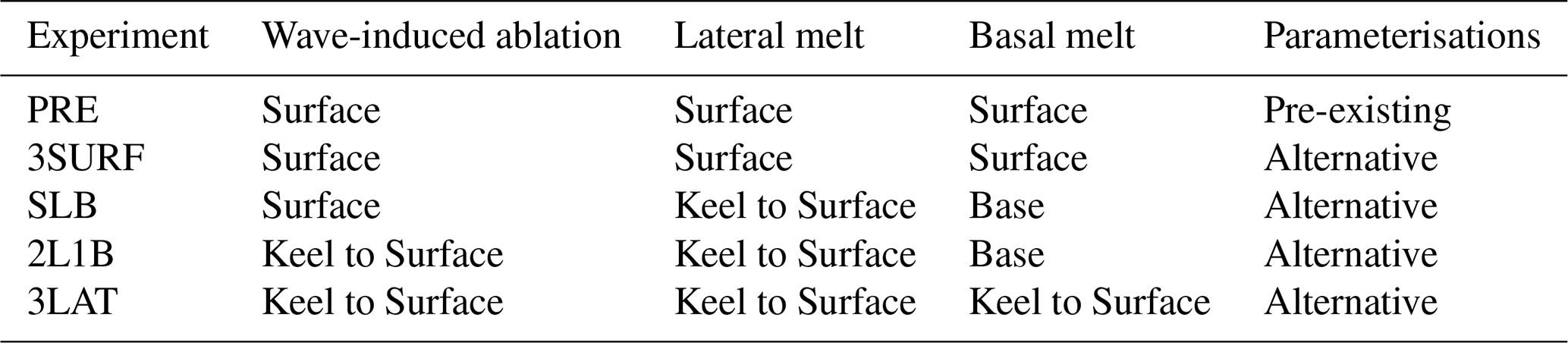
To isolate the impact of meltwater injection depth, the 3SURF serves as our reference scenario, as it uses the alternative formulation proposed here but all the melting contributions are added at the surface (Table 1). In the SLB simulation, wave-induced ablation is applied at the ocean surface, lateral melt is distributed uniformly throughout the water column up to each iceberg keel depth, and basal melt is released at the base of the iceberg. Regarding the 2L1B, the basal melt is added again at the iceberg base, and both lateral melt and wave-induced ablation are distributed uniformly throughout the water column down to the keel depth, i.e. assuming that the collapse of ice slabs above or below the wave-eroded notches plays a key role in the vertical mixing of meltwater. Finally, in 3LAT, the three melting components are redistributed together along the draft depth as an extreme case to assess the sensitivity to a fully lateral redistribution of meltwater injection. In this experiment, assumptions similar to those in 2L1B are made, except that basal melting is assumed to be entirely entrained into unresolved lateral plumes (Table 1).
The simulations use the 15-year spin-up for the REF experiment in Olivé Abelló et al. (2025). After the spin-up period, the five simulations are run for 25 years, with the first 10 years allowing the meltwater distribution from the new melting parameterisations to equilibrate and the associated surface ocean–sea-ice response to adjust, consistent with the 5–10-year adjustment of Antarctic sea ice following changes in freshwater forcing reported by Pauling et al. (2016). Annual and monthly climatologies are then computed by averaging the final 15 years of each simulation. The 15-year climatological mean total iceberg meltwater released within the domain ranges from 1195 to 1220 Gt yr−1 across experiments. Although the number of calved icebergs is identical between experiments, as it is constrained by a constant calving rate, differences in melting formulations, freshwater injection depth, and iceberg trajectories may alter local ocean temperature and salinity, creating distinct oceanic feedbacks that modulate melt rates in each experiment.
3.1 Effect of the alternative melting parameterisations on the freshwater release and iceberg lifetime
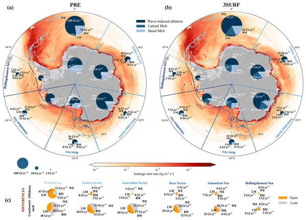
Using the alternative parameterisations (3SURF), the total iceberg freshwater flux increases by only 1.2 % relative to the pre-existing parameterisations (PRE), indicating little change in total melt between experiments (Table 2). However, their distribution reveals differences in the fraction of iceberg meltwater delivered to the open ocean and the Antarctic continental shelf across Antarctic sectors (Fig. 2). In the Weddell Sea sector, the alternative parameterisations leads to less freshwater being released over the Antarctic continental shelf, about 28 Gt yr−1 less, while the flux offshore increases substantially by 44 Gt yr−1. A similar pattern is found in the remaining sectors, but with considerably smaller magnitudes: slightly reduced freshwater over the continental shelf and increased offshore. The Amundsen Sea is an exception, showing the opposite behaviour (0.3 Gt yr−1 more freshwater released on the continental shelf and 1.4 Gt yr−1 less offshore), although the magnitude of these changes remains negligible.
Table 2Total Antarctic iceberg freshwater fluxes associated with the pre-existing (PRE) and alternative (3SURF) parameterisations, including those released over the continental shelf and offshore, also across individual Antarctic sectors, and from the different melt components. Values are expressed in Gt yr−1 together with their corresponding percentages relative to the total freshwater flux. Detailed Antarctic sectoral distributions are presented in Fig. 2.

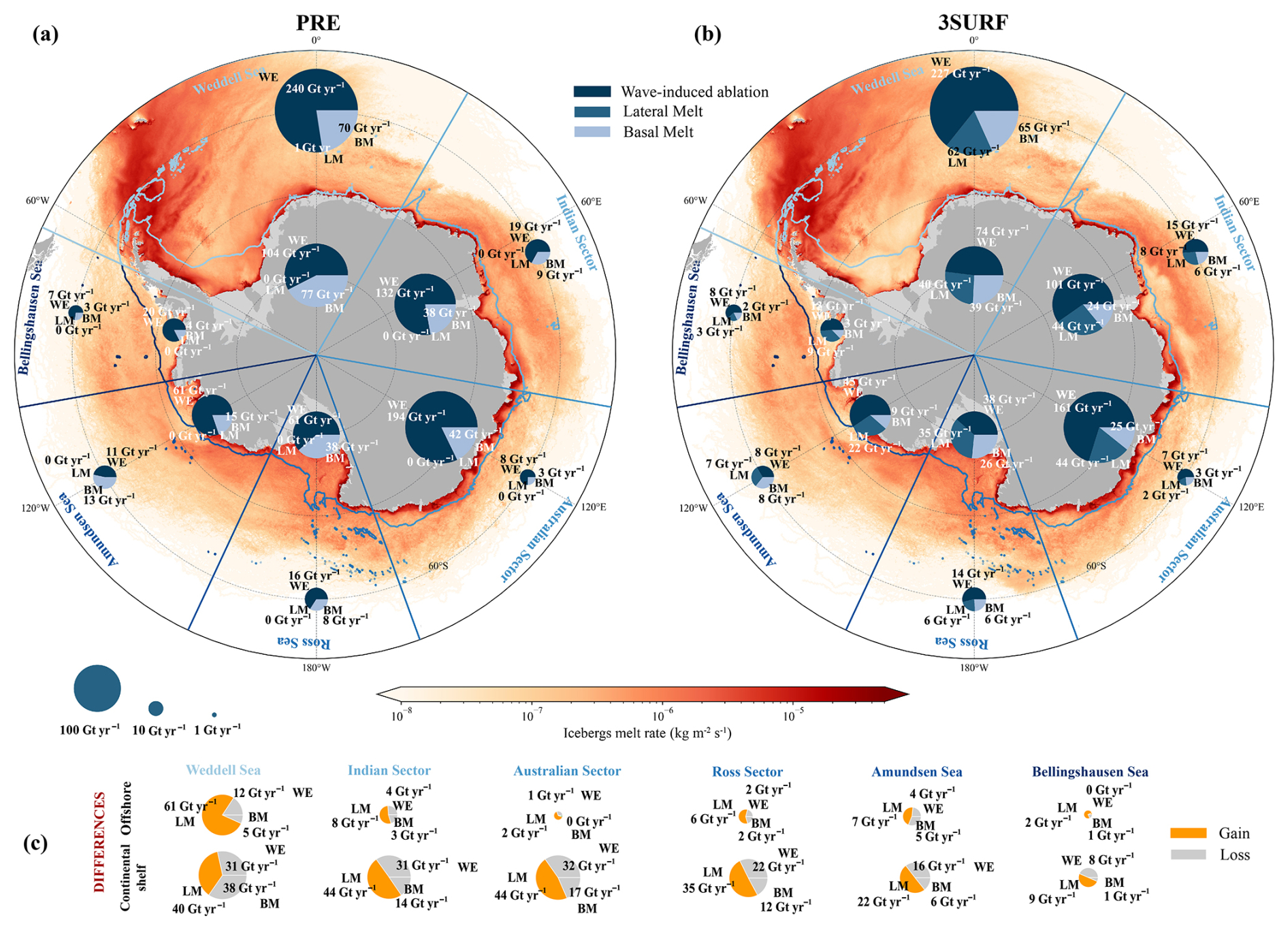
Figure 2Antarctic iceberg freshwater flux distribution averaged over the last 15 years of simulation for (a) the pre-existing NEMO parameterisations (PRE), (b) the alternative equations proposed here (3SURF), and (c) their difference (3SURF-PRE). The results are shown for six main sectors (delimited by the blue radii), and for each sector, two pie charts show the relative contributions of the three iceberg melt components: one for the continental shelf (blue contours) and one for the ocean further offshore. In the difference pie charts, orange represents gains and grey represents losses. Iceberg freshwater inputs (Gt yr−1) are composed of wave-induced ablation (WE), lateral melt (LM), and basal melt (BM), and summed as a total flux at the ocean surface.
However, the most notable change is related to the individual freshwater contribution of the melt components, especially of the lateral melt. Using the alternative parametrisations, lateral melting gains relative importance, rising from almost negligible values to become comparable to basal melting, adding a total of 24.6 % over the continental shelf and 21.3 % in the open ocean (Table 2). In contrast, basal melt remains largely unchanged in the open ocean but decreases by 11.2 % over the continental shelf. In the PRE experiment, freshwater input is clearly dominated by wave-induced ablation (73.1 %), whereas the alternative wave-erosion parameterisation substantially reduces this contribution across most Antarctic sectors, by 16.8 %–38.0 % over the continental shelf and by 5.2 %–32.0 % offshore (except in the Bellingshausen sector, where it increases slightly).
These individual melting components exhibit strong seasonal variability, peaking during the summer months (Fig. 3). Under the pre-existing parametrisations, basal and lateral melting remain largely constant throughout the year, while wave-induced ablation shows a strong seasonal decrease in austral winter (Fig. 3g), as sea-ice cover limits iceberg exposure to surface waves and also reduces the heat available for melting. In contrast, the alternative parametrisations increase the sensitivity of lateral and basal melting to ocean–sea-ice seasonality. Basal melting remains dominant in winter, but to a lesser extent than with the pre-existing parameterisations (Fig. 3g and h), while wave-induced ablation is consistently reduced throughout the year. Lateral melting becomes an important contributor in summer, exceeding basal melt in magnitude and releasing, on average, 47 Gt more freshwater than in the previous configuration.

Figure 315-year mean spatial and seasonal differences in iceberg melt rate between the pre-existing and alternative sets of parameterisations for (a–c) winter (JJA) and (d–f) summer (DJF), corresponding respectively to wave-induced ablation, lateral melt, and basal melt. Grey contours indicate the 0.35 sea-ice concentration isoline in the PRE experiment, and orange dashed contours denote the −1.8 °C isotherm depth-averaged over the upper 250 m. Positive values (red) indicate enhanced melt in the new configuration relative to the pre-existing one, and negative values (blue) indicate reduced melt. Note that, for visualisation purposes, the melt distributions are represented only south of 60° S; therefore, the net integrated differences may differ slightly considering the full Southern Ocean domain. Monthly evolution of the total freshwater mass (Gt month−1) from each melt component under the PRE (g; solid lines) and 3SURF (h; dashed lines) experiments.
Spatially, the largest positive differences occur along the Antarctic continental margins during summer, particularly in East Antarctica and the Amundsen Sea, where warm subsurface waters promote basal melting and the resulting vertical plume along the iceberg sidewalls enhances lateral melt (Fig. 3e). In winter, these positive anomalies are much more limited, persisting only at the northern tip of the Antarctic Peninsula and in Oates Land, where the water column is above the freezing point. Basal melting exhibits negative regional changes with the alternative parameterisation, showing relatively small decreases localised near and along the ice-shelf fronts in summer (with the resulting seasonal mean difference of only 3 Gt in Fig. 3g and h), and widespread negative values during winter, reaching the lowest values in the Weddell and Ross Seas where waters are found below the freezing point. In terms of wave-induced ablation, the seasonal spatial differences are almost negligible beneath the 0.35 sea-ice concentration contour both in summer and winter, and heterogeneous and pronounced in open-water regions during summer. Dividing the iceberg wave-induced ablation contribution by sectors, the reduction in 3SURF is systematic across all of them (Fig. S2). Generally, the alternative parameterisation preserves the seasonal evolution observed in PRE across all sectors, with maxima during the austral summer months and minima in winter. Over the Weddell sector, the iceberg wave-induced ablation input dominates, whereas the Australian and Indian sectors show the largest differences between experiments. The remaining Ross, Amundsen, and Bellingshausen Seas sectors receive comparatively less freshwater and exhibit a shorter ablation season (Fig. S2e–g). Overall, the new parameterisations intensify the seasonal contrast in iceberg melt, particularly over the Antarctic continental shelf, amplifying summer losses (a total mean sum of 252 Gt in 3SURF vs. 232 Gt in PRE) and further reducing winter melt (25 Gt in 3SURF and 35 Gt in PRE).

Figure 4Comparison of (a) total iceberg volume in the domain and (b) iceberg lifetime for simulations using the alternative (blue) and pre-existing (yellow) melting parameterisations. For the iceberg lifetime analysis, only those icebergs that calved and completely melted in the last 15 years of simulation for both 3SURF and PRE experiments were considered, i.e. about 28 964 particles that are equivalent to 381 634 icebergs, ensuring the same number of samples.
Enhanced lateral melting together with strong wave-induced ablation can rapidly reduce iceberg size and would therefore be expected to shorten iceberg lifetimes. However, the lifetime distribution shows the opposite behaviour, with slightly longer lifetimes under the alternative parametrisations (2.5±1.8 years compared to 2.2±1.6 years with the pre-existing scheme, Fig. 4b). This results from lower melt rates in the alternative configuration (38 m d−1 compared to 39 m d−1 in PRE), indicating slower ablation of individual icebergs. In 3SURF, wave-induced ablation is more constrained under sea-ice-covered conditions (Fig. S1), limiting lateral ablation near the Antarctic coast and allowing icebergs to survive longer and drift farther north before enhanced melting occurs in open-ocean regions. For this reason, icebergs persist longer within the domain, increasing their number and leading to an accumulation of the total ice volume (Fig. 4a). Even though the export of icebergs out of the domain is slightly higher in PRE, the difference is almost negligible (a mean of 2.27 % for PRE rather than 1.42 % for 3SURF, calculated from the residual of the mass budget). An additional contributing mechanism may be reduced basal melt, which limits iceberg thinning and favours thicker icebergs that are more prone to grounding along the continental shelf, thereby increasing retention within the 3SURF configuration.
3.2 Vertical distribution of iceberg melt
The freshwater flux has been distributed down to the keel depth of each individual iceberg, reaching different oceanic layers (Fig. 5). In the SLB experiment, 814 Gt yr−1 of freshwater flux, mostly from wave-induced ablation, are injected near the surface within the upper 10 m. In the 2L1B and 3LAT experiments, where wave-induced ablation is distributed from the surface to the keel depth, only 108 and 132 Gt yr−1 are injected in the first layer, respectively. The vertical profile of iceberg meltwater flux in these experiments is mostly located in the subsurface, with 75 % and 79 % of the meltwater released within the upper 150 m. The meltwater flux decreases sharply below, consistent with the fact that the keel depth of most icebergs lies above 300 m.

Figure 5Horizontally integrated distributions of iceberg freshwater fluxes with depth for the (a) SLB, (b) 3SURF, (c) 2L1B, and (d) 3LAT experiments. The 15-year mean total freshwater flux released in each experiment amounts to 1199, 1209, 1216, and 1220 Gt yr−1, respectively. The horizontal bars along the water column depth are distributed at 10 m intervals. Note that the x-axis is shown on a logarithmic scale.
To assess whether the injection of iceberg meltwater at depth has the potential to influence ocean layers that are isolated from the atmosphere and sea-ice forcing, we estimate the meltwater flux within and below the mixing layer, defined as the layer in which vertical mixing is active (Brainerd and Gregg, 1995). More specifically, the mixing layer in our simulations is defined as the layer above a vertical tracer diffusivity threshold of m2 s−1. In NEMO, oceanic convection is parameterised as enhanced Kz, and Kz also increases with vertical shear generated by wind or sea-ice stress. From our simulations, we estimate the maximum annual mixing layer depth (mMLD) at each grid cell, in a way to characterise the deepest layer reached by winter ventilation. In the Southern Ocean, the mMLD exhibits pronounced spatial variability, reaching the continental shelf seafloor in areas of the Ross Sea, Weddell Sea, Prydz Bay and Dumont-d'Urville Sea, which are known locations of coastal polynyas and dense water formation (Fig. S3a). This maximum typically occurs in September and October (Fig. S3b), when convection deepens the mixing layer.

Figure 6Depth-integrated iceberg freshwater (a–c) above the mMLD and (d–f) below the mMLD across the Southern Ocean for the SLB, 2L1B and 3LAT experiments. Additionally, (g–i) pie charts summarise the total freshwater input divided between offshore-water (O.W.) and continental-shelf (C.S.) regions, further separated into above (>) and below (<) mMLD contributions for each experiment. White grid cells close to the Antarctic continent denote that no freshwater is injected below the mMLD.
About three-quarters of the iceberg freshwater is released over the Antarctic continental shelf, but only between 59.2–110.1 Gt yr−1 (5 %–9 %) of that is released below the mMLD (Fig. 6g–i). Spatially, the contribution below the mMLD occurs both in areas of the continental shelf with numerous grounded icebergs (e.g. Bear Ridge in the Amundsen Sea, and in front of Berkner Island in the Weddell Sea) or further offshore in the so-called Iceberg Alley, in the north-western corner of the Weddell gyre (Fig. 6a–c). When wave-induced ablation is distributed from the surface to the iceberg keel, the contribution below the mMLD increases by 143 Gt yr−1 between the SLB and 2L1B experiments, whereas it only increases by 102 Gt yr−1 between the SLB and 3LAT experiments. The regional patterns are nonetheless similar between all experiments, indicating that the additional freshwater flux is injected into the same locations (Fig. 6a–c). In summary, most iceberg freshwater (76 %–87 %) is released above the mMLD, with 56 %–57 % occurring over the continental shelf. Indeed, substantially more freshwater penetrates below the mMLD in the open ocean than on the continental shelf, by roughly a factor of two, where mMLD is generally much shallower (Fig. S3). An exception occurs in the Pacific sector of the Southern Ocean, where mMLD reach greater depths, due to enhanced exposure to atmospheric forcing, partly modulated by large-scale atmospheric modes such as the Southern Annular Mode (SAM) and El Niño–Southern Oscillation (ENSO) (Sallée et al., 2010).
3.3 Effects on the ocean properties and ice interactions
3.3.1 Vertical distribution of water-column properties
Given that more than three-quarters of the iceberg meltwater released at depth remains within the mixing layer, we assess whether it nonetheless impacts deep-ocean properties (Fig. 7). In the SLB–3SURF comparison (Fig. 7a and d), where the differences in freshwater release between experiments are smaller and less freshwater is injected at depth (corresponding to a total of 385 Gt yr−1 redistributed from 10 m depth to the iceberg keel), substantial differences begin to emerge, particularly offshore close to the continental shelf break and most prominently in the Ross Sea sector. In particular, bottom temperature and salinity anomalies reveal a warmer and saltier dense shelf water cascading from the Ross Sea, contrasting with the colder and fresher abyssal waters nearby. Indeed, the coldest and freshest near-seafloor anomalies (highlighted by red and yellow contours, where anomalies are exceeding ±0.25 °C and ±0.05) are found over the continental shelf mainly in East Antarctica, the tip and eastern part of the Antarctic Peninsula and in the South Orkney Islands, mostly when wave-induced ablation is also redistributed from surface to icebergs' draft (Fig. 7b and e). This is consistent with enhanced subsurface meltwater delivery below the mixing layer, in particular from the numerous icebergs grounded in this sector. In contrast, in the Amundsen Sea sector, redistributing wave-induced ablation at depth results in warmer and saltier waters near the continental-shelf seafloor. The presence of particularly thick icebergs likely enhances freshwater release at greater depths, destabilising the water column, eroding the shallow mixed layer through increased turbulence, and facilitating CDW intrusion onto the continental shelf (similar to meltwater released at depth along the ice shelf base; Mathiot et al., 2017). Then, when basal melt is also redistributed from the iceberg keel to the surface, together with wave-induced ablation and lateral melt (Fig. 7c and f), several regions become warmer and saltier compared to the 2L1B experiment, including the eastern Ross Sea, the Amundsen Sea, the eastern Antarctic Peninsula–Weddell Sea sector, and Enderby Land, whereas the western Ross Sea becomes fresher and the Bellingshausen Sea exhibits slight cooling.

Figure 715-year mean bottom potential temperature and practical salinity anomaly distributions for the (a, d) SLB–3SURF, (b, e) 2L1B–3SURF, and (c, f) 3LAT–3SURF experiments. Black contours delineate two smaller subregions within the Antarctic sectors defined in Fig. 2 – the western Amundsen Sea (110–155° W) and the central Indian Ocean sector (70–100° E) – where the largest bottom continental shelf anomalies are most frequently observed. Yellow (a–c) and red (d–f) contours indicate regions where anomalies exceed ±0.25 °C and ±0.05, also highlighted by arrows, falling beyond the colourbar limits. Hatching denotes regions where mean differences are not statistically significant at the 95 % confidence level (two-sided Student's t-test applied to annual differences, 2010–2024), whereas non-hatched regions indicate robust inter-experiment differences relative to interannual variability, with the t-test providing an estimate of intrinsic variability under climatological forcing.
Although most bottom temperature and salinity anomalies are significant across the Southern Ocean, the effect of redistributing iceberg meltwater at depth on the deep ocean remains relatively small, with most anomalies remaining below ±0.2 °C and ±0.04, respectively. To assess its impact not only at the seafloor but throughout the water column, we examine seasonal mean temperature and salinity differences between 2L1B and 3SURF, which exhibit the largest difference in subsurface freshwater input (1108 Gt yr−1 redistributed below the surface). For that, we focus on two smaller subregions within the Antarctic sectors – the western Amundsen Sea and the central Indian Ocean sectors – where the largest bottom continental shelf anomalies are observed (Fig. 7).

Figure 815-year seasonal mean temperature and salinity profiles over the Antarctic continental shelf and offshore in the (a, b) central Indian Ocean and (c, d) western Amundsen Sea sectors for the 2L1B (coloured dashed lines) and 3SURF (black lines) experiments. Temperature is shown with brown lines and salinity with green lines. Note that the acronyms of DJF, MAM, JJA, and SON stand for the austral summer, spring, winter, and autumn, respectively. Shaded semi-transparent narrow bands below and around the 2L1B profiles indicate 95 % confidence interval of the seasonal mean, computed from the 15-year seasonal mean profiles (2010–2024) using Student's t distribution. Insets show the corresponding freshwater flux (Gt per season) released over each domain (continental shelf or open ocean) for the 2L1B and 3SURF experiments. The boundaries of the two smaller sectors are shown in Fig. 7.
The seasonal mean temperature and salinity profiles for these two Antarctic sectors, both for open waters and over the continental shelf up to 600 m can be found in Fig. 8. Offshore, the depth at which iceberg freshwater is injected barely alters surface salinity and temperature in both sectors, with maximum reductions of about 0.03 and 0.04 °C at the surface of the western Amundsen Sea when less freshwater is injected, while changes in the Indian Ocean sector are almost negligible (these seasonal differences can be observed in greater detail in Fig. S4). Instead, when iceberg freshwater is discharged on the Antarctic continental shelf in the central Indian Ocean sector, higher surface salinity and temperature are observed in austral summer and autumn when the wave-induced meltwater is redistributed at depth rather than injected at the surface. At depth, a subsurface shift occurs, with colder, fresher waters appearing from approximately 50 m for temperature and 50–175 m for salinity, depending on the season, and extending downward to the seafloor. These subsurface anomalies dominate, with temperature decreases of about 0.1 °C and salinity reductions of about 0.02. In the western Amundsen Sea sector, the surface temperature pattern is quite similar, but surface salinity is slightly lower when the freshwater is redistributed at depth. Below the surface and down to 350 m, a slightly colder and fresher layer develops when freshwater is injected at depth, likely influenced by an enhanced Antarctic ice-shelf meltwater plume that spreads along the continental shelf. Around 250–300 m, both temperature and salinity profiles show a marked transition where subsurface iceberg freshwater input ends. At depth, there is a shift in terms of salinity, starting to be saltier at depths below 350 m and also warmer at the bottom by 0.1 °C. These opposing vertical anomalies highlight how the depth at which iceberg freshwater is released modifies the stratification and bottom tracer structure over the shelf.
Therefore, as more freshwater is added to the subsurface, the bottom waters over the East Antarctic continental shelf and the western Ross Sea are colder and fresher, also partly due to the inflow of fresher waters onto the shelves, which increases the sea surface height (not shown). In contrast, in the Amundsen Sea, the release of iceberg meltwater at depth, rather than reducing the density contrast between surface and deep layers, is associated with an increase in temperature below the mixed layer (Fig. 8d). This suggests that subsurface freshwater input may modify the stratification and reduce vertical heat exchange with the surface, allowing heat to persist at depth, potentially enhanced by the presence of relatively warm CDW intruding onto the shelf through submarine channels. Overall, the effects throughout the water column remain weak, both offshore and over the continental shelf, even when most of the iceberg freshwater flux is injected below the surface.
3.3.2 Sea-ice distribution
In terms of sea-ice production (Fig. 9), enhanced sea ice formation is found over the Antarctic continental shelf when iceberg meltwater is injected at subsurface levels. By redistributing freshwater throughout the water column, subsurface meltwater enhances vertical mixing, promoting more efficient heat loss to the atmosphere, maintaining open-water areas free of ice (Fig. 9g–i), and intensifying sea-ice production within coastal polynyas. As a result, sea-ice production over the Antarctic continental shelf is enhanced when iceberg meltwater is injected at subsurface levels (Fig. 9a–c). As more water is redistributed along the water column, slightly more sea ice is produced, (0.4±0.29) %, (1.9±0.36) %, and (2.2±0.37) % for SLB, 2L1B and 3LAT, respectively (where the standard deviation is computed across years to quantify intrinsic variability).

Figure 9Difference in the 15-year mean distribution of (a–c) sea-ice production, (d–f) sea-ice thickness, and (g–i) sea-ice concentration for the SLB, 2L1B, and 3LAT simulations relative to the 3SURF simulation. Hatching denotes regions where mean differences are not statistically significant at the 95 % confidence level (two-sided Student's t-test applied to annual differences, 2010–2024). Note that hatched regions also include areas beyond the sea-ice production/thickness coverage, where values are absent. The names of the ice shelves located near the largest anomalies are indicated in (e) as a reference.
Although sea-ice production contributes to sea-ice thickness thermodynamically, the two components do not necessarily have to share the same spatial patterns, as thickness is also controlled by sea-ice export, convergence or divergence processes, and mechanical redistribution (Vancoppenolle et al., 2023). One example is coastal polynyas, where high sea-ice production can remain characterized by thin ice or open water because newly formed ice is continuously exported. Comparing sea-ice production with Fig. 9d–f, regions of thinner sea ice coincide locally with elevated sea-ice production, particularly on the southern side of Drygalski Ice Tongue and in the vicinity of the Prince Harald and Larsen D ice shelves. Hence, reduced surface freshwater injection promotes thinner sea ice, expanded open-water regions, and, eventually, more active coastal polynyas, where efficient heat loss to the atmosphere enables continuous sea-ice formation. In contrast, in front of the western side of Ross Ice Shelf (southern side of Drygalski Ice Tongue), where no persistent coastal polynya is present, injecting iceberg freshwater at depth rather than at the surface weakens the near-surface haline stratification (as reflected by the localised positive sea-surface temperature and salinity anomalies shown in Fig. S5). This weakening favours a more vertically mixed upper ocean, which, together with recurrent leads (reflected in the negative sea-ice concentration anomalies) and strong offshore katabatic winds, likely enhances sea-ice export, thereby limiting sea-ice thickening. Consistent with this mechanism, Fig. S6 suggests enhanced northward sea-ice volume export along the coastal region south of the Drygalski Ice Tongue as more meltwater is injected at subsurface levels, while sea-ice divergence anomalies are spatially heterogeneous and do not exhibit a clear spatial pattern. In general, this highlights thinner sea ice in the Weddell Sea, which is often overestimated in some NEMO configurations where iceberg meltwater is released exclusively at the surface, leading some studies to even limit unrealistic sea-ice growth (Pirlet et al., 2025). In particular, the volume of the entire sea ice cover (averaged over March–October) exhibits a modest decline of 192 (1.6 %), 141 (1.1 %), and 105 km3 (0.9 %) for SLB, 2L1B and 3LAT, respectively.
For sea-ice concentration (Fig. 9g–i), localised reductions occur along parts of the Antarctic continental margin, while sea-ice concentration increases considerably over broad parts of the seasonal ice zone in open-ocean waters, particularly in the Pacific sector. These coastal decreases partly coincide with regions of reduced ice thickness, suggesting stronger ice divergence and a higher presence of leads and larger open-water fractions despite sustained local ice formation. In 3LAT, the anomalies are predominantly more negative and spatially heterogeneous, indicating a greater reduction in sea-ice concentration across parts of the seasonal ice zone. Indeed, the sea-ice extent increases slightly by 61×103 km2 (0.35 %) and 65×103 km2 (0.38 %) in SLB and 2L1B, respectively, while decreasing by 29×103 km2 (0.17 %) in 3LAT.
3.3.3 Ice-shelves melting
Ice-shelf melt responses are highly contrasted between the central Indian Ocean and western Amundsen Sea sectors across all subsurface freshwater injection experiments (Fig. 10). Relative to the 3SURF configuration, ice-shelf melt rates are reduced in the Indian Ocean sector, consistent with a cooler ocean environment, with mean decreases of approximately 3.1, 7.9, and 8.0 Gt yr−1 (4.4 %, 11.4 %, and 11.5 %) for the SLB, 2L1B, and 3LAT experiments, respectively. In contrast, the Amundsen sector (Fig. 10c, d, and f) shows an enhancement of ice-shelf melt rates, increasing by about 2.7, 10.5, and 13.5 Gt yr−1 (1.2 %, 4.8 %, and 6.1 %) in the same simulations. Hence, ice shelves in the Indian Ocean sector exhibit a greater relative sensitivity to subsurface meltwater from icebergs, although the overall changes remain modest, especially for Amundsen ice shelves. These contrasting melt responses result from the pronounced regional differences in the vertical structure of ocean properties and upper-ocean mixing (Fig. S4). In the western Amundsen Sea, ice shelves are exposed to warmer and saltier surroundings, favouring enhanced basal melt. Due to the relatively shallower mixed layer (Fig. S5), thicker icebergs may release freshwater below, promoting localised turbulence and vertical mixing that can weaken stratification and facilitate intrusions of CDW to shallow depths. In contrast, the central Indian Ocean sector is characterised by fresher and colder waters in front of the Amery, West and Shackleton ice shelves, from west to east, leading to reduced basal melting. In this sector, subsurface freshwater injection occurs within the mixed layer and limits oceanic heat access to the ice-shelf base, as it exhibits a deeper mixed layer compared to the western Amundsen Sea and generally thinner icebergs (Olivé Abelló et al., 2025). Nevertheless, the overall impact of redistributing iceberg meltwater at depth on Antarctic ice-shelf melt rates remains comparatively weak. Even in the experiments showing the largest differences in subsurface freshwater release (Fig. 10b and e), the simulated changes remain small relative to the total ice-shelf basal melt fluxes, especially in the western Amundsen Sea compared to the central Indian Ocean sector, highlighting the limited large-scale sensitivity of ice shelves to the vertical redistribution of iceberg freshwater.

Figure 10Difference in the 15-year mean distribution of ice-shelf melt flux for the (a–c) central Indian Ocean and (d–f) western Amundsen Sea sectors for the SLB, 2L1B, and 3LAT simulations relative to the 3SURF simulation. In grey are labelled the main Antarctic ice shelves in the regions, and in grey contours are represented the 1000, 2000, and 3000 m isobaths.
In this study, we have revisited the representation of Antarctic iceberg melting in a circum-Antarctic configuration by implementing alternative melt parameterisations. In the first NEMO simulations representing icebergs and considering the two hemispheres, Marsh et al. (2015) showed that wave-induced ablation was the dominant process (81.4 %), whereas the basal melt contributed substantially less (18.2 %), and the sidewall melt was negligible (0.4 %). Developments of the iceberg module since then (Merino et al., 2016; Olivé Abelló et al., 2025), together with the focus on the Southern Ocean, have changed these ratios to 73.1 %, 26.8 %, and 0.1 %, respectively. Currently, the alternative parameterisations implemented in this work further change these ratios to 58.8 %, 17.9 %, and 23.3 %, respectively. Hence, the dominance of wave-induced ablation is robust across the two sets of parameterisations. Additionally, the updated parameterisations modify the seasonal cycle of freshwater release, increasing the fraction of annual iceberg meltwater released in austral summer (DJF) from 43 % (Merino et al., 2016) to 62 %.
4.1 Limitations of the parameterisations and experimental design
More sophisticated formulations (e.g. Huth et al., 2022) could further improve the representation of wave erosion (Mamer and Robel, 2026), or represent the wave-induced iceberg fragmentation and the melting of ice fragments in a more physically based approach. FitzMaurice and Stern (2018) have discussed in detail the caveats of the two representations of basal melting used in this study, concluding that the three-equation formulation is not well suited for small icebergs, which are too short to develop a well-mixed ocean layer beneath the iceberg base. The fact that drifting icebergs tend to move together with the surrounding ocean (Kostov et al., 2026) may also limit turbulence and reinforce this caveat. We therefore acknowledge that our basal melt rates may be overestimated, and future work should explore alternative basal melt formulations following the recommendations of FitzMaurice and Stern (2018). Assuming that basal melt feeds the lateral plumes along the iceberg walls has a large impact on the melt partitioning, but the validity of this assumption remains uncertain and depends on whether the relative ocean–iceberg velocity is high enough to detach basal melt from the iceberg.
Beyond the limitations in the melt formulations, the relatively short duration of the sensitivity experiments may represent an additional caveat. While 10 years is sufficient for the upper ocean and sea ice to adjust, ongoing evolution of abyssal hydrography indicates that the 25 yr simulations are not sufficiently long for the deep ocean and associated feedbacks to fully equilibrate (not shown). Indeed, achieving full deep-ocean equilibrium can require spin-up and simulation periods of hundreds to thousands of years (e.g. Zhang et al., 2025; de Lavergne et al., 2026). However, over the Antarctic continental shelf, the Amundsen Sea, the western Ross Sea and the western Weddell Sea tend towards stabilisation, especially in the last 15 years (Fig. S7). As bottom temperature and salinity share similar trends across experiments, incomplete stabilisation may have limited impact on bottom-property anomalies.
Also, we have prescribed the vertical distribution of each melt component down to the iceberg keel without explicitly investigating how the ocean–iceberg relative velocity may affect the detachment of meltwater from icebergs (FitzMaurice et al., 2017). Nevertheless, our set of experiments describes the extreme cases, from all meltwater released at the surface to meltwater redistributed from the keel to the surface. Therefore, more complex vertical meltwater distributions are expected to fall within the range explored in this study.
4.2 Ocean response to meltwater depth and contrasts with the Arctic
Overall, we find a small effect of releasing iceberg meltwater at depth rather than at the ocean surface. Annual mean bottom-temperature anomalies remain below 0.2 °C across most of the Antarctic continental shelf, reaching localised maxima of +0.5 °C in the western Amundsen Sea and −0.3 °C in the central Indian Ocean sector (Fig. 7a–c). Practical salinity anomalies are similarly small, generally remaining within This weak and spatially confined response partly reflects the rapid dilution of iceberg meltwater, with daily temperature and salinity anomalies remaining highly localised and dissipating within a few days (Appendix B), consistent with recent in situ observations around large tabular icebergs (Lucas et al., 2025).
Although these hydrographic anomalies are generally small, changes of comparable magnitude have been associated with variability in Antarctic Bottom Water (AABW) volume transport. In the Australian Antarctic Basin, Gunn et al. (2023) reported AABW salinity changes of 0.04 g kg−1 during 1992–2011 and 0.03 g kg−1 during 2011–2018, associated with a decrease of 4.4 Sv and a recovery of 2.2 Sv, respectively. In our experiments, the increase in net Dense Shelf Water export (DSW, a precursor of AABW) across the Ross Sea continental shelf-break section was only 0.075 Sv (4.3 %; Fig. S8). Thus, while iceberg-meltwater injection at depth can locally modify shelf hydrography, these anomalies do not translate into a comparably strong DSW export response.
This weak impact of releasing iceberg meltwater at depth may be specific to the Southern Ocean and may not apply to the Northern Hemisphere. Indeed, Amaral Wasielesky (2025) reported a stronger impact of vertically distributing the melt of Greenlandic icebergs. They simulated maximum temperature anomalies ranging from 0.5 to 1 °C and salinity changes reaching 0.15 in deeper layers, driving significant large-scale circulation changes in the Arctic. Variations in Arctic–Antarctic ocean response can be attributed mainly to differences in mixed-layer depth and tabular iceberg thicknesses. On the one hand, the summer mixed layer may be thinner in some parts of the Arctic region than around Antarctica. On the other hand, the iceberg thickness distribution differs between the Arctic/North Atlantic and the Southern Ocean: in Antarctica, icebergs inherit their thickness from large and thick floating ice shelves (Olivé Abelló et al., 2025), while most icebergs in the Northern Hemisphere calve from grounded tidewater glaciers in Greenlandic fjords (Mouginot et al., 2019).
A similar contrast emerges when comparing iceberg meltwater with ice-shelf meltwater released at depth around Antarctica (Mathiot et al., 2017; Thomas et al., 2023) despite comparable total mass fluxes (Rignot et al., 2013; Davison et al., 2023). A first explanation is that ice shelves do not drift, so their meltwater is continuously released at the same location, leading to stronger local buoyancy at depth. A second explanation is that ice shelves melt the most in their deepest parts, typically between 500–1000 m (e.g. Rignot et al., 2013), while icebergs are calved with a mean thickness of 220 m (Olivé Abelló et al., 2025, Fig. S5).
4.3 Relevance of representing iceberg freshwater release at depth
Ocean modellers may wonder which of the iceberg melt vertical distributions used in this article they should implement. The SLB experiment likely provides the most realistic combination of the vertical distribution of iceberg meltwater, as the different melt processes are represented consistently with the characteristic depth at which each melt mechanism occurs. However, the actual vertical distribution of iceberg meltwater remains poorly constrained, and further observations in the vicinity of icebergs, as well as dedicated high-resolution modelling, would be needed to improve its vertical distribution. In a strongly stratified water column, basal melt can remain partially trapped at the keel depth for some time before being advected away or mixed upward. Nevertheless, the large-scale ocean response is weak regardless of where iceberg freshwater is injected within the water column, with our most physically consistent configuration (SLB) producing changes of only 1.2 %–4.4 % in ice-shelf melt rates, about 0.4 % in sea-ice production, and approximately 1.6 % in sea-ice volume. These results suggest that, at large scales, prescribing iceberg meltwater entirely at the surface only introduces small biases in the simulated Southern Ocean state.
We implemented more physics-based parameterisations for Antarctic iceberg basal, lateral, and wave-induced melting in the NEMO ocean–sea-ice model, including an explicit representation of meltwater release at depth along the iceberg draft. Across Antarctic sectors, iceberg melt is dominated by wave-induced ablation, followed by basal and lateral melting. Under the updated parameterisation, the contribution of lateral melting increases substantially, from negligible values to accounting for about 23 % of the total freshwater flux, while wave-induced ablation decreases from 70 %–60 %. As a result, both wave-induced ablation and basal melt are slightly reduced, especially during austral winter. Hence, the updated melting parameterisations amplify the seasonal contrast in iceberg melt, with an increase in summer melt (27 Gt month−1) and a reduction in winter melt (10 Gt month−1).
Despite redistributing iceberg meltwater vertically, the freshwater flux remains strongly surface-intensified, with approximately 76 %–87 % released within the maximum annual mixed layer, primarily because most Antarctic icebergs are relatively thin compared with the mixed-layer depth, especially over the Antarctic continental shelf. Nevertheless, the fraction of meltwater injected below the mixed layer produces localised but statistically significant changes in bottom temperature and salinity, particularly over the continental shelf and in regions of deep winter mixing. These subsurface freshwater inputs lead to contrasting regional responses: slight cooling and freshening of bottom waters in East Antarctica and the western Ross Sea, and slight warming and salinification of shelf bottom waters in the Amundsen Sea, where iceberg freshwater injected below the mixed-layer depth, together with enhanced ice shelf melt (Fig. 10), promotes increased vertical mixing, weakens the local stratification, and facilitates intrusions of modified CDW onto the continental shelf. However, the oceanic response to the different vertical distributions of iceberg meltwater remains small throughout the full water column, including near-bottom waters, particularly offshore.
The updated freshwater distribution also affects sea-ice formation, promoting thinner sea ice mainly in the Weddell Sea. Regions of reduced sea ice thickness generally coincide with enhanced sea-ice production and reduced sea-ice concentration. Across all subsurface-injection experiments, sea-ice production increases slightly, while total Antarctic sea-ice volume simultaneously declines. In parallel, ice-shelf melt responses exhibit a clear regional contrast: basal melt decreases in the central Indian Ocean sector, whereas it increases in the western Amundsen sector. These opposing responses are consistent with the simulated changes in bottom temperature and salinity, with colder and fresher shelf waters limiting oceanic heat access in the Indian Ocean region, and warmer, saltier conditions enhancing basal melting in the Amundsen Sea. This contrast underscores the strong sensitivity of ice-shelf mass balance to the vertical structure of freshwater input.
Finally, at surface and daily scales, iceberg meltwater discharge promotes local temperature and salinity anomalies that are rapidly diluted within a few days, consistent with observations near large tabular Antarctic icebergs, where meltwater-induced signals decay quickly away from the iceberg and do not persist beyond the immediate vicinity.
Overall, our results show that, because iceberg meltwater remains widely distributed across the Southern Ocean and is primarily confined to the Antarctic mixed layer, its impact on the full water column is limited. Despite explicitly representing a wide range of physically plausible melting combinations – SLB, 2L1B, and 3LAT –, the resulting bottom anomalies remain spatially confined and moderate in magnitude. Although the SLB experiment likely provides the most realistic and physics-based vertical distribution of iceberg meltwater, prescribing all iceberg meltwater at the surface, as done in many iceberg–ocean modelling studies to date (e.g. Merino et al., 2016; Olivé Abelló et al., 2025), may still represent an acceptable approximation for large-scale ocean simulations in the Southern Ocean. Nevertheless, injecting iceberg meltwater at depth is recommended, particularly in regional studies focusing on dense water formation and biogeochemical processes.
To determine the salinity and temperature profile tendencies, we first estimate the ice volume loss associated with iceberg melting. Essentially, the new iceberg length and/or width, Xn, result from the reduction of the lateral dimensions due to wave-induced ablation and lateral melting processes according to . Similarly, the new thickness is computed as . Then, the associated volume loss is given by . Depending on the experimental setup (see Sect. 2.3), each of the melting components can be either transferred to the same vertical grid cell layer (at the surface or iceberg keel depth) or redistributed uniformly throughout the water column. Then, the melted ice volume in the corresponding vertical level, ΔVk in m3, is converted into an equivalent freshwater volumetric flux profile by dividing by the time step and multiplying by ice-to-seawater density ratio, thereby determining the freshwater flux that dilutes ocean salinity (in m3 s−1). The salinity tendency formulation corresponds to a virtual freshwater flux, whereby iceberg melting modifies the local tracer properties without explicitly adding iceberg mass to the ocean. It is therefore expressed as:
where Δt is the model time step, Sijk is the local ocean salinity, Ahij is the horizontal grid-cell area, and e3tijk is the height of the grid cell. Similarly, the temperature tendency has two contributions: the dilution by cold meltwater, and the heat balance associated with the melting process (sensible and latent heat):
where Tijk is the local ocean temperature (K), cp the specific heat capacity (J K−1), Lf the latent heat of fusion of ice (J kg−1), and Tz the freezing point (K).
The weak response of mean bottom-ocean properties to iceberg meltwater injection at depth can be partly attributed to its rapid dilution in the ocean. Analysing them at smaller spatial scales and daily temporal resolution, higher melt rates are associated with fresher and colder water properties in the iceberg grid-cell positions, affecting only the individual cell and showing no detectable response in the surrounding cells. This is consistent with vertical measurements near the A68 tabular iceberg (Lucas et al., 2025), where casts located more than 5.5 km from the edge of the berg did not exhibit any temperature–salinity intrusions. Between affected and non-affected locations (at 2.6 and 7 km, respectively), the maximum anomalies were of 0.2 g kg−1 and 0.1 °C at the upper 20 m, whereas the anomalies around and below the iceberg draft depth were reaching 0.1 g kg−1 and 0.25–0.3 °C. In our simulations, these local surface changes are below 0.03 °C and 0.02 g kg−1 per day and do not persist beyond five days, as shown in Fig. B1. Indeed, in Fig. B1e, temperature anomalies referenced to the pre-melting state decay rapidly, indicating that the thermal signal associated with iceberg meltwater injection is short-lived. In contrast, in terms of salinity (Fig. B1d), no clear decay timescale emerges, as the response to iceberg meltwater injection is largely masked by the strong internal variability of the salinity field. As the icebergs analysed in Fig. B1 are free-drifting, grounded icebergs would be expected to generate larger anomalies, more consistent with Lucas et al. (2025) and with those shown in Fig. S4 over the continental shelf.

Figure B1Spatial and temporal response of the ocean to surface iceberg melting. Maps of consecutive daily differences for the 3SURF experiment for (a) sea surface salinity, (b) sea surface temperature (°C), and (c) iceberg melt rate (). Coloured dashed lines indicate the evolution of iceberg's trajectory, with markers showing daily positions; black dots together with black squares highlight the grid cells where iceberg melt is assessed exceeding the applied threshold (). Time series of the anomalies for the same sampled grid cell (black squares) along the time relative to day 0 for (e) temperature, (d) salinity, and (f) melt rate.
The new code developments for the NEMO iceberg module will be uploaded and documented, and will be publicly available at the GitLab repository: https://forge.nemo-ocean.eu/ (last access: 2 November 2026). Additionally, the original code for the vertical distribution of iceberg melting used as a basis for these developments is available at http://www.github.com/YavorKostov/Iceberg_basal_melt (last access: 13 December 2024) and https://doi.org/10.5281/zenodo.23900361 (Kostov, 2026).
The monthly WOA23 dataset used for comparison is available in open access at https://www.ncei.noaa.gov/access/world-ocean-atlas-2023/ (last access: 17 September 2026). The resulting dataset from this study is publicly available on Zenodo under the following https://doi.org/10.5281/zenodo.23474735 (Olivé Abelló et al., 2026). It includes the 15-year annual and monthly climatologies of the three-dimensional iceberg meltwater flux distribution for all experiments, covering the entire Southern Ocean south of 52.25° S, both in absolute and normalized terms.
The supplement related to this article is available online at https://doi.org/10.5194/os-22-3747-2026-supplement.
Conceptualisation: AOA, PM, NJ, PH. Data curation: AOA, PH. Formal analysis: AOA. Funding acquisition: NJ. Investigation: YK, PH. Methodology: AOA, PM, YK. Project administration: NJ. Resources: NJ. Software: AOA, PM, YK. Supervision: PM, NJ, PH. Validation: AOA, NJ. Writing – original draft: AOA. Writing – review and editing: PM, NJ, YK, PH.
The contact author has declared that none of the authors has any competing interests.
Publisher's note: Copernicus Publications remains neutral with regard to jurisdictional claims made in the text, published maps, institutional affiliations, or any other geographical representation in this paper. The authors bear the ultimate responsibility for providing appropriate place names. Views expressed in the text are those of the authors and do not necessarily reflect the views of the publisher.
This work was granted access to the high-performance computing (HPC) resources of TGCC under allocation A0140106035 attributed by GENCI. The authors are very grateful to the editor, Julian Mak, and to the two referees, one anonymous and Robert Marsh, for their many useful comments and suggestions, which helped to improve the manuscript.
This research was supported by Ocean Cryosphere Exchanges in ANtarctica: Impacts on Climate and the Earth system, OCEAN ICE, which is funded by the European Union, Horizon Europe Funding Programme for research and innovation under grant agreement no. 101060452, https://doi.org/10.3030/101060452. OCEAN ICE contribution number 56. This work was funded by UK Research and Innovation (UKRI) under the UK government's Horizon Europe funding Guarantee (grant number 10048443). This study has received funding from Agence Nationale de la Recherche – France 2030 as part of the PEPR TRACCS programme under grant numbers ANR-22-EXTR-0008 (IMPRESSION-ESM) and ANR-22-EXTR-0010 (ISClim).
This paper was edited by Julian Mak and reviewed by R. Marsh and one anonymous referee.
Abib, N., Sutherland, D. A., Peterson, R., Catania, G., Nash, J. D., Shroyer, E. L., Stearns, L. A., and Bartholomaus, T. C.: Ice mélange melt changes observed water column stratification at a tidewater glacier in Greenland, The Cryosphere, 18, 4817–4829, https://doi.org/10.5194/tc-18-4817-2024, 2024. a
Ackermann, L., Rackow, T., Himstedt, K., Gierz, P., Knorr, G., and Lohmann, G.: A comprehensive Earth system model (AWI-ESM2.1) with interactive icebergs: effects on surface and deep-ocean characteristics, Geosci. Model Dev., 17, 3279–3301, https://doi.org/10.5194/gmd-17-3279-2024, 2024. a
Amaral Wasielesky, G.: Parameterizing the release of iceberg meltwater at depth: impacts on the Subpolar North Atlantic, Master's thesis, Department of Environment and Geography, University of Manitoba, Canada, http://hdl.handle.net/1993/39399 (last access: 12 January 2026), 2025. a, b
Asay-Davis, X. S., Cornford, S. L., Durand, G., Galton-Fenzi, B. K., Gladstone, R. M., Gudmundsson, G. H., Hattermann, T., Holland, D. M., Holland, D., Holland, P. R., Martin, D. F., Mathiot, P., Pattyn, F., and Seroussi, H.: Experimental design for three interrelated marine ice sheet and ocean model intercomparison projects: MISMIP v. 3 (MISMIP +), ISOMIP v. 2 (ISOMIP +) and MISOMIP v. 1 (MISOMIP1), Geosci. Model Dev., 9, 2471–2497, https://doi.org/10.5194/gmd-9-2471-2016, 2016. a, b
Bigg, G. R., Wadley, M. R., Stevens, D. P., and Johnson, J. A.: Modelling the dynamics and thermodynamics of icebergs, Cold Reg. Sci. Technol., 26, 113–135, https://doi.org/10.1016/S0165-232X(97)00012-8, 1997. a, b, c, d
Brainerd, K. E. and Gregg, M. C.: Surface mixed and mixing layer depths, Deep-Sea Res. Pt. I, 42, 1521–1543, https://doi.org/10.1016/0967-0637(95)00068-H, 1995. a
Cenedese, C. and Straneo, F.: Icebergs melting, Annu. Rev. Fluid Mech., 55, 377–402, https://doi.org/10.1146/annurev-fluid-032522-100734, 2023. a
Davison, B. J., Hogg, A. E., Gourmelen, N., Jakob, L., Wuite, J., Nagler, T., Greene, C. A., Andreasen, J., and Engdahl, M. E.: Annual mass budget of Antarctic ice shelves from 1997 to 2021, Science Advances, 9, eadi0186, https://doi.org/10.1126/sciadv.adi0186, 2023. a
de Lavergne, C., Rathore, S., Madec, G., Sallée, J.-B., Ethé, C., Nasser, A., Millet, B., and Vancoppenolle, M.: Effects of improved tidal mixing in NEMO one-degree global ocean model, J. Adv. Model. Earth Sy., 18, e2024MS004824, https://doi.org/10.1029/2024MS004824, 2026. a
Depoorter, M. A., Bamber, J. L., Griggs, J. A., Lenaerts, J. T., Ligtenberg, S. R., van den Broeke, M. R., and Moholdt, G.: Calving fluxes and basal melt rates of Antarctic ice shelves, Nature, 502, 89–92, https://doi.org/10.1038/nature12567, 2013. a
Dowdeswell, J. A. and Bamber, J. L.: Keel depths of modern Antarctic icebergs and implications for sea-floor scouring in the geological record, Mar. Geol., 243, 120–131, https://doi.org/10.1016/j.margeo.2007.04.008, 2007. a
El-Tahan, M., Venkatesh, S., and El-Tahan, H.: Validation and quantitative assessment of the deterioration mechanisms of Arctic icebergs, J. Offshore Mech. Arct., 102–108, https://doi.org/10.1115/1.3256983, 1987. a, b, c
FitzMaurice, A. and Stern, A.: Parameterizing the basal melt of tabular icebergs, Ocean Model., 130, 66–78, https://doi.org/10.1016/j.ocemod.2018.08.005, 2018. a, b, c
FitzMaurice, A., Cenedese, C., and Straneo, F.: Nonlinear response of iceberg side melting to ocean currents, Geophys. Res. Lett., 44, 5637–5644, https://doi.org/10.1002/2017GL073585, 2017. a, b, c
Gladstone, R. M., Bigg, G. R., and Nicholls, K. W.: Iceberg trajectory modeling and meltwater injection in the Southern Ocean, J. Geophys. Res.-Oceans, 106, 19903–19915, https://doi.org/10.1029/2000JC000347, 2001. a, b, c, d, e
Gunn, K. L., Rintoul, S. R., England, M. H., and Bowen, M. M.: Recent reduced abyssal overturning and ventilation in the Australian Antarctic Basin, Nat. Clim. Change, 13, 537–544, https://doi.org/10.1038/s41558-023-01667-8, 2023. a
Helly, J. J., Kaufmann, R. S., Stephenson Jr, G. R., and Vernet, M.: Cooling, dilution and mixing of ocean water by free-drifting icebergs in the Weddell Sea, Deep-Sea Res. Pt. II, 58, 1346–1363, https://doi.org/10.1016/j.dsr2.2010.11.010, 2011. a
Hester, E. W., McConnochie, C. D., Cenedese, C., Couston, L.-A., and Vasil, G.: Aspect ratio affects iceberg melting, Physical Review Fluids, 6, 023802, https://doi.org/10.1103/PhysRevFluids.6.023802, 2021. a, b, c
Holland, D. M. and Jenkins, A.: Modeling thermodynamic ice–ocean interactions at the base of an ice shelf, J. Phys. Oceanogr., 29, 1787–1800, https://doi.org/10.1175/1520-0485(1999)029<1787:MTIOIA>2.0.CO;2, 1999. a, b
Huth, A., Adcroft, A., and Sergienko, O.: Parameterizing tabular-iceberg decay in an ocean model, J. Adv. Model. Earth Sy., 14, e2021MS002869, https://doi.org/10.1029/2021MS002869, 2022. a
Jenkins, A.: The impact of melting ice on ocean waters, J. Phys. Oceanogr., 29, 2370–2381, https://doi.org/10.1175/1520-0485(1999)029<2370:TIOMIO>2.0.CO;2, 1999. a
Jenkins, A., Nicholls, K. W., and Corr, H. F.: Observation and parameterization of ablation at the base of Ronne Ice Shelf, Antarctica, J. Phys. Oceanogr., 40, 2298–2312, https://doi.org/10.1175/2010JPO4317.1, 2010. a
Jongma, J. I., Driesschaert, E., Fichefet, T., Goosse, H., and Renssen, H.: The effect of dynamic–thermodynamic icebergs on the Southern Ocean climate in a three-dimensional model, Ocean Model., 26, 104–113, https://doi.org/10.1016/j.ocemod.2008.09.007, 2009. a
Jourdain, N. C., Mathiot, P., Merino, N., Durand, G., Le Sommer, J., Spence, P., Dutrieux, P., and Madec, G.: Ocean circulation and sea-ice thinning induced by melting ice shelves in the Amundsen Sea, J. Geophys. Res.-Oceans, 122, 2550–2573, https://doi.org/10.1002/2016JC012509, 2017. a
Jourdain, N. C., Mathiot, P., Burgard, C., Caillet, J., and Kittel, C.: Ice shelf basal melt rates in the Amundsen Sea at the end of the 21st century, Geophys. Res. Lett., 49, e2022GL100629, https://doi.org/10.1029/2022GL100629, 2022. a
Kobayashi, S., Ota, Y., Harada, Y., Ebita, A., Moriya, M., Onoda, H., Onogi, K., Kamahori, H., Kobayashi, C., Endo, H., MIYAOKA, K., and TAKAHASHI, K.: The JRA-55 reanalysis: general specifications and basic characteristics, J. Meteorol. Soc. Jpn., 93, 5–48, https://doi.org/10.2151/jmsj.2015-001, 2015. a
Kostov, Y.: YavorKostov/Iceberg_basal_melt: 2 (Version 2), Zenodo [code], https://doi.org/10.5281/zenodo.23900361, 2026. a
Kostov, Y., Holland, P. R., Hogan, K. A., Smith, J. A., Jourdain, N. C., Mathiot, P., Olivé Abelló, A., Fleming, A. H., and Meijers, A. J. S.: Modelled dynamics of floating and grounded icebergs, with application to the Amundsen Sea, The Cryosphere, 20, 135–169, https://doi.org/10.5194/tc-20-135-2026, 2026. a, b
Lucas, N. S., Brearley, J. A., Hendry, K. R., Spira, T., Braakmann-Folgmann, A., Abrahamsen, E. P., Meredith, M. P., and Tarling, G. A.: Giant iceberg meltwater increases upper-ocean stratification and vertical mixing, Nat. Geosci., 1–8, https://doi.org/10.1038/s41561-025-01659-7, 2025. a, b, c, d
Madec, G. and the NEMO System Team: NEMO ocean engine (v4.2), Zenodo [code], https://doi.org/10.5281/zenodo.6334656, 2022. a, b
Mamer, M. and Robel, A.: Buoyancy feedbacks on wave-induced melting of icebergs, J. Geophys. Res.-Oceans, 131, e2025JC023273, https://doi.org/10.1029/2025JC023273, 2026. a
Marsh, R., Ivchenko, V. O., Skliris, N., Alderson, S., Bigg, G. R., Madec, G., Blaker, A. T., Aksenov, Y., Sinha, B., Coward, A. C., Le Sommer, J., Merino, N., and Zalesny, V. B.: NEMO–ICB (v1.0): interactive icebergs in the NEMO ocean model globally configured at eddy-permitting resolution, Geosci. Model Dev., 8, 1547–1562, https://doi.org/10.5194/gmd-8-1547-2015, 2015. a
Martin, T. and Adcroft, A.: Parameterizing the fresh-water flux from land ice to ocean with interactive icebergs in a coupled climate model, Ocean Model., 34, 111–124, https://doi.org/10.1016/j.ocemod.2010.05.001, 2010. a, b, c, d, e, f
Mathiot, P. and Jourdain, N. C.: Southern Ocean warming and Antarctic ice shelf melting in conditions plausible by late 23rd century in a high-end scenario, Ocean Sci., 19, 1595–1615, https://doi.org/10.5194/os-19-1595-2023, 2023. a, b
Mathiot, P., Jenkins, A., Harris, C., and Madec, G.: Explicit representation and parametrised impacts of under ice shelf seas in the z* coordinate ocean model NEMO 3.6, Geosci. Model Dev., 10, 2849–2874, https://doi.org/10.5194/gmd-10-2849-2017, 2017. a, b
Merino, N., Le Sommer, J., Durand, G., Jourdain, N. C., Madec, G., Mathiot, P., and Tournadre, J.: Antarctic icebergs melt over the Southern Ocean: climatology and impact on sea ice, Ocean Model., 104, 99–110, https://doi.org/10.1016/j.ocemod.2016.05.001, 2016. a, b, c, d, e
Moorman, R., Thompson, A. F., Youngs, M. K., and Stewart, A. L.: The Antarctic coastal ocean heat budget is dominated by heat loss to land ice melt, Science Advances, 12, eaec7443, https://doi.org/10.1126/sciadv.aec7443, 2026. a
Morlighem, M.: MEaSUREs BedMachine Antarctica, Version 3, Boulder, Colorado USA, NASA National Snow and Ice Data Center Distributed Active Archive Center [data set], https://doi.org/10.5067/FPSU0V1MWUB6, 2022. a
Morlighem, M., Rignot, E., Binder, T., Blankenship, D., Drews, R., Eagles, G., Eisen, O., Ferraccioli, F., Forsberg, R., Fretwell, P., Goel, V., Greenbaum, J. S., Gudmundsson, H., Guo, J., Helm, V., Hofstede, C., Howat, I., Humbert, A., Jokat, W., Karlsson, N. B., Lee, W. S., Matsuoka, K., Millan, R., Mouginot, J., Paden, J., Pattyn, F., Roberts, J., Rosier, S., Ruppel, A., Seroussi, H., Smith, E. C., Steinhage, D., Sun, B., van den Broeke, M. R., van Ommen, T. D., van Wessem, M., and Young, D. A.: Deep glacial troughs and stabilizing ridges unveiled beneath the margins of the Antarctic ice sheet, Nat. Geosci., 13, 132–137, https://doi.org/10.1038/s41561-019-0510-8, 2020. a
Mouginot, J., Rignot, E., Bjørk, A. A., Van den Broeke, M., Millan, R., Morlighem, M., Noël, B., Scheuchl, B., and Wood, M.: Forty-six years of Greenland Ice Sheet mass balance from 1972 to 2018, P. Natl. Acad. Sci. USA, 116, 9239–9244, https://doi.org/10.1073/pnas.1904242116, 2019. a
Naughten, K. A., Holland, P. R., Dutrieux, P., Kimura, S., Bett, D. T., and Jenkins, A.: Simulated twentieth-century ocean warming in the Amundsen Sea, West Antarctica, Geophys. Res. Lett., 49, e2021GL094566, https://doi.org/10.1029/2021GL094566, 2022. a
Nose, T., Waseda, T., Kodaira, T., and Inoue, J.: Satellite-retrieved sea ice concentration uncertainty and its effect on modelling wave evolution in marginal ice zones, The Cryosphere, 14, 2029–2052, https://doi.org/10.5194/tc-14-2029-2020, 2020. a
Olivé Abelló, A., Mathiot, P., Jourdain, N. C., Kostov, Y., Holland, P. R., Gascoin, S., and Rousset, C.: Iceberg grounding enhances the release of freshwater on the Antarctic continental shelf, J. Geophys. Res.-Oceans, 130, e2025JC022857, https://doi.org/10.1029/2025JC022857, 2025. a, b, c, d, e, f, g, h, i, j, k, l
Olivé Abelló, A., Mathiot, P., Jourdain, N., Kostov, Y., and Holland, P.: Olivé Abelló et al., 2026 dataset – Simulated Antarctic iceberg melting occurs primarily within the Southern Ocean mixed layer, Zenodo [data set], https://doi.org/10.5281/zenodo.23474735, 2026. a
Pauling, A. G., Bitz, C. M., Smith, I. J., and Langhorne, P. J.: The response of the Southern Ocean and Antarctic sea ice to freshwater from ice shelves in an Earth system model, J. Climate, 29, 1655–1672, https://doi.org/10.1175/JCLI-D-15-0501.1, 2016. a
Pirlet, N., Fichefet, T., Vancoppenolle, M., Fraser, A. D., Mathiot, P., Rousset, C., Barthélemy, A., Barriat, P.-Y., Pelletier, C., Madec, G., and Kittel, C.: Benefits of a landfast ice representation on simulated Antarctic sea ice and coastal polynya dynamics, J. Geophys. Res.-Oceans, 130, e2024JC022032, https://doi.org/10.1029/2024JC022032, 2025. a
Rackow, T., Wesche, C., Timmermann, R., Hellmer, H. H., Juricke, S., and Jung, T.: A simulation of small to giant A ntarctic iceberg evolution: differential impact on climatology estimates, J. Geophys. Res.-Oceans, 122, 3170–3190, https://doi.org/10.1002/2016JC012513, 2017. a
Rignot, E., Jacobs, S., Mouginot, J., and Scheuchl, B.: Ice-shelf melting around Antarctica, Science, 341, 266–270, https://doi.org/10.1126/science.1235798, 2013. a, b, c
Rignot, E., Xu, Y., Menemenlis, D., Mouginot, J., Scheuchl, B., Li, X., Morlighem, M., Seroussi, H., den Broeke, M. v., Fenty, I., Cai, C., An, L., and Fleurian, B. d.: Modeling of ocean-induced ice melt rates of five west Greenland glaciers over the past two decades, Geophys. Res. Lett., 43, 6374–6382, https://doi.org/10.1002/2016GL068784, 2016. a, b
Rintoul, S. R., Silvano, A., Pena-Molino, B., Van Wijk, E., Rosenberg, M., Greenbaum, J. S., and Blankenship, D. D.: Ocean heat drives rapid basal melt of the Totten Ice Shelf, Science Advances, 2, e1601610, https://doi.org/10.1126/sciadv.1601610, 2016. a
Rintoul, S. R., Van Wijk, E. M., Herraiz-Borreguero, L., and Rosevear, M. G.: Circulation and ocean–ice shelf interaction beneath the Denman and Shackleton Ice Shelves, Science Advances, 11, eadx1024, https://doi.org/10.1126/sciadv.adx1024, 2025. a
Sallée, J.-B., Speer, K., and Rintoul, S.: Zonally asymmetric response of the Southern Ocean mixed-layer depth to the Southern Annular Mode, Nat. Geosci., 3, 273–279, https://doi.org/10.1038/ngeo812, 2010. a
Sartore, N. B., Wagner, T. J. W., Siegfried, M. R., Pujara, N., and Zoet, L. K.: Wave erosion, frontal bending, and calving at Ross Ice Shelf, The Cryosphere, 19, 249–265, https://doi.org/10.5194/tc-19-249-2025, 2025. a, b, c, d
Savage, S.: Aspects of iceberg deterioration and drift, in: Geomorphological fluid mechanics, Springer, https://doi.org/10.1007/3-540-45670-8_12, 279–318, 2001. a, b, c
Scambos, T., Sergienko, O., Sargent, A., MacAyeal, D., and Fastook, J.: ICESat profiles of tabular iceberg margins and iceberg breakup at low latitudes, Geophys. Res. Lett., 32, https://doi.org/10.1029/2005GL023802, 2005. a
Silva, T., Bigg, G., and Nicholls, K.: Contribution of giant icebergs to the Southern Ocean freshwater flux, J. Geophys. Res.-Oceans, 111, https://doi.org/10.1029/2004JC002843, 2006. a, b, c
Slater, D. A., Felikson, D., Straneo, F., Goelzer, H., Little, C. M., Morlighem, M., Fettweis, X., and Nowicki, S.: Twenty-first century ocean forcing of the Greenland ice sheet for modelling of sea level contribution, The Cryosphere, 14, 985–1008, https://doi.org/10.5194/tc-14-985-2020, 2020. a, b
Slater, D. A., Johnstone, E., Mas e Braga, M., Fraser, N. J., Cowton, T., and Inall, M.: FjordRPM v1.0: a reduced-physics model for efficient simulation of glacial fjords, Geosci. Model Dev., 18, 7475–7500, https://doi.org/10.5194/gmd-18-7475-2025, 2025. a
Thomas, M., Ridley, J. K., Smith, I. J., Stevens, D. P., Holland, P. R., and Mackie, S.: Future response of Antarctic continental shelf temperatures to ice shelf basal melting and calving, Geophys. Res. Lett., 50, e2022GL102101, https://doi.org/10.1029/2022GL102101, 2023. a
Vancoppenolle, M., Rousset, C., Blockley, E., Aksenov, Y., Feltham, D., Fichefet, T., Garric, G., Guémas, V., Iovino, D., Keeley, S., Madec, G., Massonnet, F., Ridley, J., Schroeder, D., and Tietsche, S.: SI3, the NEMO Sea Ice Engine, Zenodo [code], https://doi.org/10.5281/zenodo.7534900, 2023. a
Wagner, T. J., Wadhams, P., Bates, R., Elosegui, P., Stern, A., Vella, D., Abrahamsen, E. P., Crawford, A., and Nicholls, K. W.: The “footloose” mechanism: iceberg decay from hydrostatic stresses, Geophys. Res. Lett., 41, 5522–5529, https://doi.org/10.1002/2014GL060832, 2014. a
Wagner, T. J., Dell, R. W., Eisenman, I., Keeling, R. F., Padman, L., and Severinghaus, J. P.: Wave inhibition by sea ice enables trans-Atlantic ice rafting of debris during Heinrich events, Earth Planet. Sc. Lett., 495, 157–163, https://doi.org/10.1016/j.epsl.2018.05.006, 2018. a
Weeks, W. F. and Campbell, W.: Icebergs as a fresh-water source: an appraisal, J. Glaciol., 12, 207–233, https://doi.org/10.3189/S0022143000032044, 1973. a, b
Weiss, K. J., Nash, J. D., Wengrove, M. E., Osman, N., Cohen, N. F., Jackson, R. H., Pettit, E. C., Zhao, K. X., Nahorniak, J. S., and Sutherland, D. A.: Direct measurement of glacier ice melt: boundary layer details are critical for submarine melt prediction at near-vertical ice faces, Geophys. Res. Lett., 52, e2025GL114952, https://doi.org/10.1029/2025GL114952, 2025. a
White, F. M., Spaulding, M. L., and Gominho, L.: Theoretical estimates of the various mechanisms involved in iceberg deterioration in the open ocean environment. Tech. Rep. CG-D-62-80, U.S. Coast Guard Off. Res. Dev., Washington, DC, 1980. a, b
Wiskandt, J. and Jourdain, N. C.: Brief communication: Representation of heat conduction into ice in marine ice shelf melt modelling, The Cryosphere, 19, 3253–3258, https://doi.org/10.5194/tc-19-3253-2025, 2025. a
Zhang, J., Zhang, X., King, M. A., and Lyu, K.: The response of the Southern ocean to Climatological iceberg freshwater forcing, Clim. Dynam., 63, 440, https://doi.org/10.1007/s00382-025-07922-2, 2025. a
- Abstract
- Introduction
- Methodology
- Results
- Discussion
- Conclusions
- Appendix A: Salinity and temperature profiles tendencies
- Appendix B: Rapid spatial dilution and short-lived persistence of iceberg meltwater anomalies
- Code and data availability
- Author contributions
- Competing interests
- Disclaimer
- Acknowledgements
- Financial support
- Review statement
- References
- Supplement
- Abstract
- Introduction
- Methodology
- Results
- Discussion
- Conclusions
- Appendix A: Salinity and temperature profiles tendencies
- Appendix B: Rapid spatial dilution and short-lived persistence of iceberg meltwater anomalies
- Code and data availability
- Author contributions
- Competing interests
- Disclaimer
- Acknowledgements
- Financial support
- Review statement
- References
- Supplement