Blue carbon development and ecosystem services in oligotrophic environments: the case for a shallow coastal installation on the shelf off Tenerife (Canary Islands)

This study assessed the unplanned ecosystem services provided by a submarine monitoring station over 18 months, including an environmental characterisation of a shallow coastal shelf area off SW Tenerife (Canary Islands), a calculation of the benthic biomass developed (the generated blue carbon) and the identification of the species pool related to the installation, representing the associated biodiversity. The oligotrophic coastal waters at the studied site permitted a benthic biomass generation between 1.02 and 2.88 g m⁻², and a carbon sequestration between 0.24 and 0.40 g m⁻². Furthermore, 46 species belonging to 11 phyla were identified during 4 periodical monitoring dives. The ecosystem services provided by the monitoring station included primary production, carbon sequestration, fish nursery and shelter (regulating ecosystem service). The installation also benefited the biodiversity maintenance (regulating and maintenance ecosystem service). The environmental conditions (physical, chemical and biological) at the studied site were not a limiting factor for benthic biomass development. The amount of blue carbon generated was lower compared to the main blue carbon ecosystems (e.g., seagrass meadows, mangroves and salt marshes) and high-latitude (polar) ecosystems, but similar to Mediterranean gorgonian-based ecosystems. Our study demonstrates that the present oligotrophic study site is a good candidate for benthic ecosystem restoration due to its facility for blue carbon development and provision of ecosystem services.

1 Introduction

Healthy ecosystems provide goods and services that contribute to human well-being; these benefits are known as ecosystem services (De Groot et al., 2002; Khan, 2020; Mengist et al., 2020). These services are grouped into three categories, namely, provisioning (e.g., food, construction materials, primary production), regulating and maintenance (e.g., climate regulation-carbon sequestration, coastal protection and stabilization, fish nursery, habitat provisioning, nutrient cycling), cultural (e.g., recreational and tourism, education) (Czúcz et al., 2018; Friess et al., 2020; Millenium Ecosystem Assessment, 2005). Biodiversity is not specifically regarded as an ecosystem service, rather as a fundamental provider for each of the other services. For example, biodiversity influences and supports the adequate functioning of several ecosystem services such as oxygen and food production, nutrient cycling, carbon absorption and storage, among others.

Marine benthic biomass development is also known as blue carbon, referring to the atmospheric carbon captured and retained in marine living organisms in the ocean and coastal ecosystems (Nellemann et al., 2009). It also includes the carbon sequestered in the living and non-living biomasses within sea floor sediment (McLeod et al., 2011). Blue carbon can be stored for short term (e.g., tens of years) in biomass and over longer time scales (e.g., thousands of years) in sediments (Duarte et al., 2005; Lo Iacono et al., 2008). Among the largest carbon stocks in coastal environments are seagrass meadows of Posidonia oceanica and mangroves. These systems can generate carbon-rich sediments more than 10 m deep and more than 6000 years old (Lo Iacono et al., 2008; Mckee et al., 2007; Serrano et al., 2014).

Anthropogenic pressures such as the overexploitation of resources, habitat loss and degradation and pollution, among many others, drastically affect ecosystem services (Campagne et al., 2023). Climate change and particularly, ocean acidification and warming are especially dangerous due to the large spatial extent of their impacts (Gutt et al., 2015; Campagne et al., 2023). The World Economic Forum (2020) estimated that USD 44 trillion of economic value generation, that represent more than half of the world's total Gross Domestic Product (GDP), is moderately or highly dependent on nature and its services (e.g., ecosystem services) and therefore exposed to risks derived from the ongoing anthropogenic nature alteration. The large economic impact of ecosystem services and biodiversity degradation is undeniable.

The growing concern about climate change and the degradation of the marine environment has launched many conservation and restoration projects worldwide. The present study is part of the Horizon Europe project OCEAN CITIZEN (https://www.oceancitizen.eu, last access: 28 October 2026), which aims to develop a replicable marine restoration protocol, combining carbon immobilization, habitat and biodiversity regeneration with social engagement and economic benefits for local communities. As part of this effort, a submarine environmental monitoring station was installed off the SW coast of Tenerife Island (Canary Islands, Atlantic Ocean). Tenerife has the highest population density in the Canary Islands and significant population growth and urban development in coastal areas (Gayá Vilar et al., 2024). Tourism has led to an exponential increase in anthropogenic pressures on the territory, such as changes in land uses, resource consumption, degradations of ecosystems and pollution (Millenium Ecosystem Assessment, 2005). Pollution from waste water discharge is one of the greatest impacts on the local marine environment (Herrera et al., 2020; Lozano et al., 2016). Due to the convergence of several anthropogenic impacts, the degraded coastal ecosystem to the south of Tenerife has been proposed as a target site for benthic regeneration efforts within the OCEAN CITIZEN project. Within this frame, a coastal submarine environmental monitoring station was installed to record the environmental characteristics of this coastal, shallow and oligotrophic site.

In this study, we provide an assessment of blue carbon development, biodiversity characteristics and ecosystem services associated to the installation of a submarine environmental monitoring station after 18 months of operation, together with some aspects of their relationships to the environmental parameters that enabled such unexpected benthic growth in an oligotrophic coastal area.

2 Methods

2.1 Study area

The coastal waters to the south of Tenerife are oligotrophic, under the influence of water filaments detaching from the Canary Current Upwelling System (Sangrà, 2015). A quasi-permanent thermocline prevents the entrance of nutrients into the surface mixed layer. However, wind mixing of surface waters during the winter erodes the thermocline and allows nutrient in the upper water column stimulating phytoplankton growth (Braun, 1980; Cianca et al., 2007; De León and Braun, 1973). This winter state coincides with the highest annual intensity of atmospheric iron inputs produced by the frequent African dust resuspension events, locally named as “calima”, which could be a factor enhancing winter primary production (Sarthou et al., 2007; Viana et al., 2002; Torres-Padrón et al., 2002; Gelado et al., 2003; Dorta et al., 2005, Suárez et al., 2021). Nevertheless, annual primary production peaks during summer in the Canary Islands region, coinciding with trade winds and light intensity maxima (Gómez-Letona et al., 2017). Chlorophyll a concentration increases from April to August and decreases from August to October, which is consistent with the seasonal relationship between nutrient availability and phytoplankton blooms development and evolution in coastal regions (Cloern, 1996; Ramírez et al., 2005; Winder and Cloern, 2010).

There are no studies on blue carbon development in this area; however, its proximity to the Canary Current Upwelling System, calima-derived iron fertilization and the consequent phytoplankton blooms, and the presence of submarine outfalls may provide sufficiently favourable conditions for benthic assemblages to develop. The closest 2 of the 208 submarine outfalls known in Tenerife are approximately located 1 km to the North and 1 km to the South of the monitoring station, at the lee and current-ward positions of the submarine installation. These submarine outfalls are classified as unauthorised by the Canary Islands government, implying that there is no control on their emissions.

2.2 Oceanographic conditions

An instrumented submarine structure was installed at 25.5 m water depth, on the continental shelf off the SW coast of Tenerife ($\mathrm{28}\mathit{°}{\mathrm{12}}^{\prime }{\mathrm{27.7}}^{\prime \prime }$ N, $\mathrm{16}\mathit{°}{\mathrm{50}}^{\prime }{\mathrm{25.8}}^{\prime \prime }$ W) on 12 September 2023 (Figs. 1 and 2). Temperature, chlorophyll a, turbidity, light, dissolved O₂ and current velocity and direction were measured from 15 September 2023 to 10 March 2025. The observation period was interrupted from 24 to 25 April and from 2 to 3 September 2024, due to equipment maintenance. Temperature, chlorophyll a and turbidity measurements were acquired using a JFE-Alec Infinity CLW (model ACLW-USB) taking 240 data d⁻¹. The accuracy of the measurements of this sensor were ±1 % for chlorophyll a, ±0.3 FTU or 2 % for turbidity and ±0.02 °C for temperature. This sensor took 10 consecutives reading per hour; therefore, chlorophyll a and turbidity data were averaged hourly to homogenize data. Chlorophyll a and turbidity records showed intermittent irregular values; therefore, chlorophyll a values above 20 µg L⁻¹ and negatives values were discarded. The turbidity measurements taken at the same time as the discarded chlorophyll a values were also removed. Altogether, these discarded data represented less than 3 % of the data collection of each variable and were probably related to obstructions of the sensors or unusual malfunctions of the instrument. Salinity measurements were acquired every 30 min using a Star Oddi CTD (Model DST). The accuracy of the salinity measurement was ±1. Light (visible light spectrum) was measured 48 times per day with a HOBO^® Pendant^® MX Water Temp/Light (MX2202) sensor. The accuracy of the light measurement was ±10 % in direct sunlight conditions. Dissolved oxygen (DO) data were acquired using a JFE Rinko W (Model AROW-USB), reading 216 times per day. The accuracy of the dissolved oxygen measurement was ±2 % at full scale range. Water current speed and direction were measured every minute with a Lowell Instruments TCM1 current meter. The accuracy of the current speed measurement was between 2–3 cm s⁻¹, and 5° of accuracy for the current direction measurement. The station included a fiberglass 90 cm height and 130 cm diameter Technicap PPS4 sediment trap, with an external surface area of 32 270 cm², measured in the laboratory.

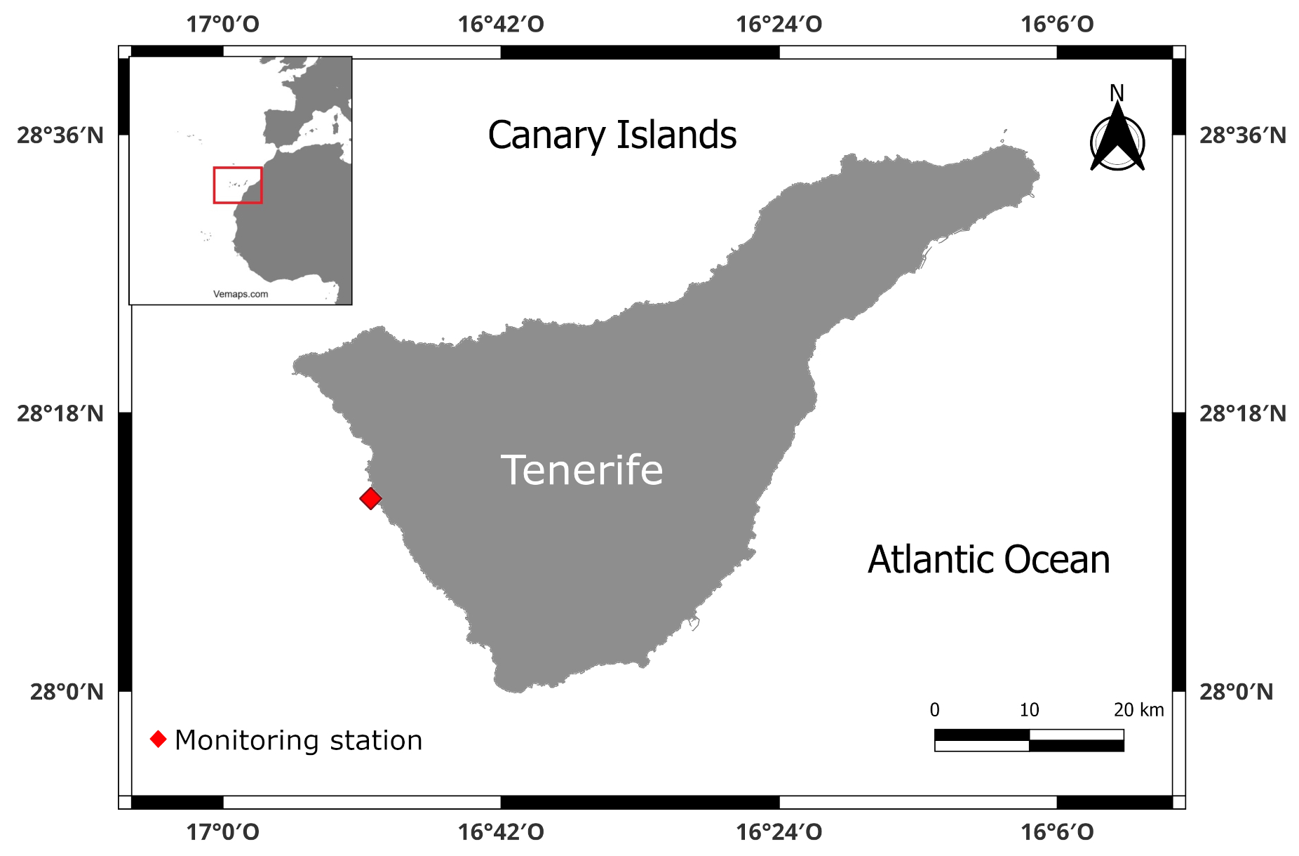
Figure 1 Map of the study area (Tenerife, Canary Island) and the location of the monitoring station. The data provided for the production of this map were provided by European Marine Observation and Data Network (EMODnet).

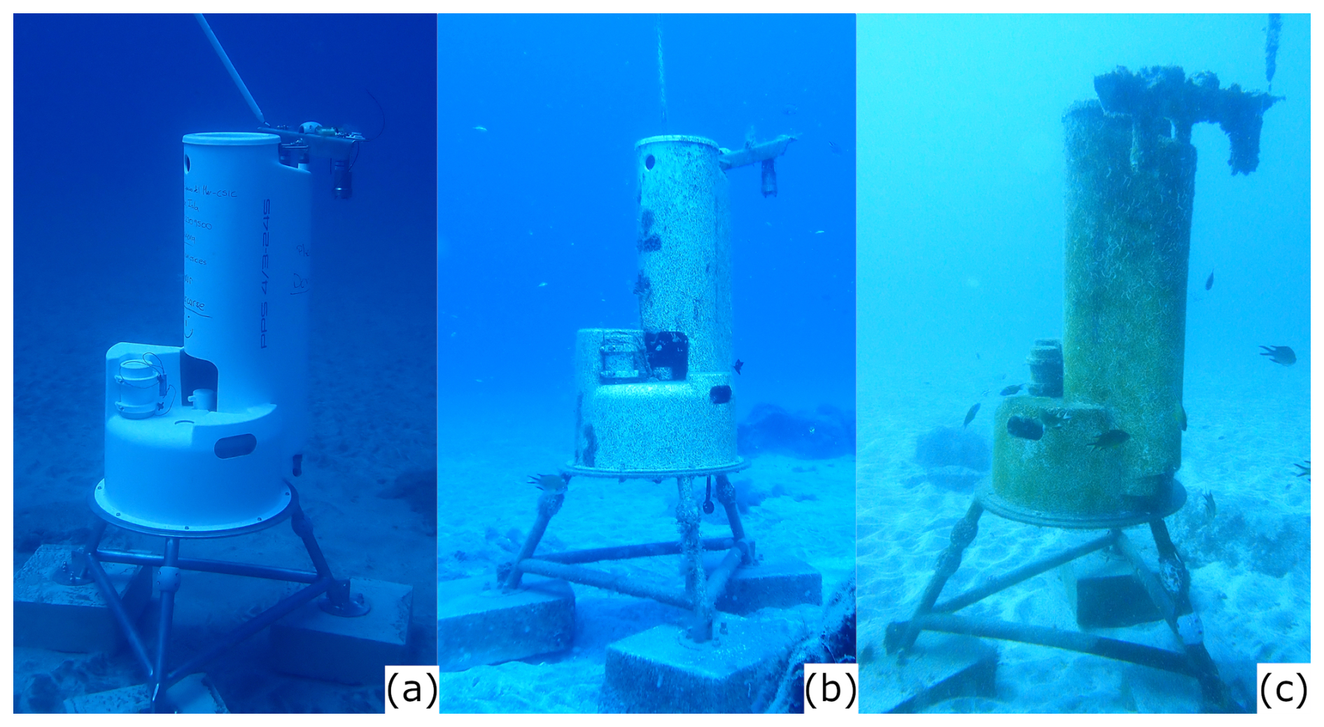
Figure 2 (a) station the day of deployment (12 September 2023), (b) station after 9 months – 267 d of deployment (6 June 2024) and (c)station after 18 months – 544 d after deployment (11 March 2025). Photos by: Isabelle Peeters.

2.3 Satellite observations

2.3.1 Chlorophyll

8 d averaged chlorophyll a concentration images with a spatial resolution of 4 km spanning all the study period were obtained and downloaded from NASA Aqua MODIS satellite data Internet site (https://oceancolor.gsfc.nasa.gov/l3/, last access: 27 March 2025). The chlorophyll a values correspond to the area delimited by the coordinates: 33° N, 8° W, 23° N, 22° W, which includes the study area, the Canary Islands and the Canary Current Upwelling zone. MODIS-derived chlorophyll concentration at 4 km tends to overestimate in the nearshore waters as shown by a high mean relative percentage difference of 77 % (Harshada et al., 2021).

2.3.2 Aerosol Optical Depth

8 d Aerosol optical depth (AOD) satellite images (were obtained from NASA Aqua MODIS Satellite Internet site (NASA Earth Observation, https://neo.gsfc.nasa.gov/view.php?datasetId=MYDAL2_E_AER_OD&year=2024, last access: 27 March 2025). Images were provided by Aqua MODIS Satellite. The AOD measurements uncertainty (i.e. theoretical error) over ocean is ±0.03–0.05 (Remer et al., 2002). AOD is the relative measure of the proportion of scattered and/or absorbed radiation along the entire atmospheric vertical column, from the sensor on the satellite to the Earth's surface. This radiation can be attenuated by aerosols (e.g., urban haze, smoke particles, desert dust, sea salt). Due to the proximity of the Canary Islands to the African continent and the relevance that the resuspended Saharan dust has on ocean fertilization, AOD was taken into account as an environmental parameter for the assessment of blue carbon development. These images enabled correlating the abundance of African dust in the air or calima, chlorophyll a and turbidity measured in situ at the station, where benthic biomass samples were taken. The dates when calima affected the Canary Islands were selected to explore data correlations. Calima data were obtained from AEMET (Agencia Estatal de Meteorología, Spain) monthly reports (https://www.aemet.es/es/serviciosclimaticos/vigilancia_clima/resumenes, last access: 27 March 2025) and from the visual inspection of satellite images.

2.4 Biomass

Benthic biomass samples were collected from the fiberglass surface. The collection of samples was done by SCUBA diving, carefully scrapping the biomass incrusted over a surface of 400 cm² (20 cm × 20 cm square) on 24 April 2024 (7 months (226 d), after station's deployment), defined as Time 7 (T₇), 3 September 2024 (12 months (356 d) after station's deployment), defined as Time 12 (T₁₂) and 10 March 2025 (18 months (544 d) after station's deployment), defined as Time 18 (T₁₈). This methodology enabled monitoring the evolution of benthic biomass development over the entire study period (Fig. 2). Moreover, the same square sampled on T₇, was sampled again in T₁₂. This enabled the observation of recolonization between T₇ and T₁₂ (almost 5 months – e.g., 130 d of development). The development of benthic biomass growth was labelled as B and the biomass recolonization between T₇ and T₁₂ as R (Fig. 3). Thus, the four biomass growth periods over the fibre glass surface will be reported here as BT₇, BT₁₂, BT₁₈ and RT₁₂.

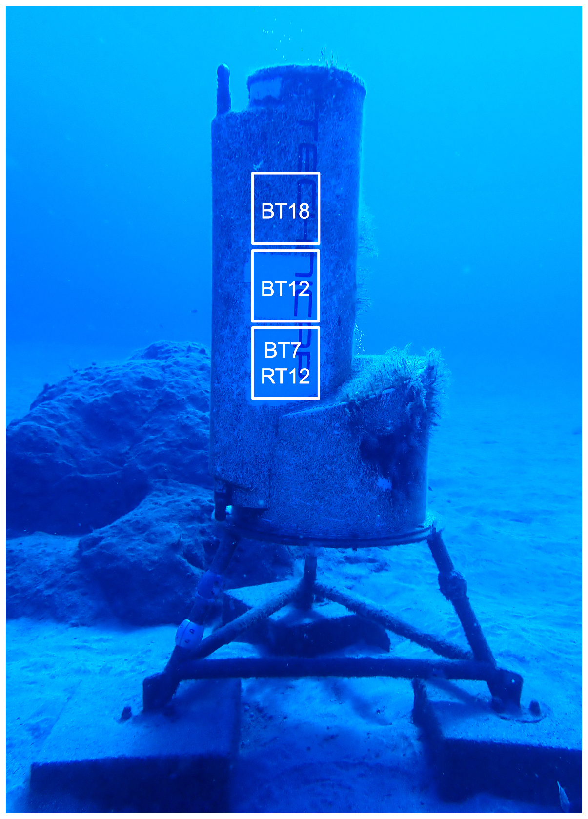
Figure 3 Benthic biomass squares sampled in the different times: BT₇ (April 2024), BT₁₂ (September 2024), BT₁₈ (March 2025) and RT₁₂ (September 2024). Photos by: Isabelle Peeters.

Samples were collected in zip-lock plastic bags and frozen at −20 °C for transport. Sample biomass losses occurred during collection and transport due to sample buoyancy and plastic bag leakage during on-deck manipulation; therefore, the biomass values reported here represent the minimum values of biomass growth, particularly those values corresponding to BT₁₂, RT₁₂ and BT₁₈, when working underwater was very difficult due to the water current strength that hampered diver's stability and winnowed biomass samples.

Samples were freeze-dried during 24 h. Before filtering, samples were rinsed to eliminate salts with distilled water in a beaker. Then, samples were filtered through pre-combusted (at 400 °C for 12 h) and pre-weighted (with 0.00001 g precision) 47 mm GF/F Whatman glass fibre filters. These filters were dried at 40 °C during 24 h in an oven. Filters were placed in a desiccator during 3 h before weighting. To achieve constant weight, weighing procedure was repeated for 5 d.

2.5 Organic Carbon

The biomass samples retained onto filters were digested with 37 % HCl during 48 h in a closed recipient inside a fume hood at room temperature to remove carbonates. After digestion, the glass fibre filters with biomass were placed in an oven during 24 h at 40 °C. Once they were dry, filters were placed in a desiccator during 3 h before weighing. To achieve constant weight, weighing was repeated during 5 d. Filters were combusted in a LECO Truspec CN analyser, results are expressed in weight %. The organic carbon (OC) mass was calculated from the total dry weight of the sample before acidic digestion.

2.6 Biodiversity and benthic colonization

A visual census of diversity classified as colonizing (algae and sessile benthic fauna fixed onto the sediment trap body), associated (motile species living by the submarine station) and pelagic (swimming) species, was carried out at the beginning of each monitoring dive. The various surveys were defined as, T₇ (April 2024), T₉ (June 2024), T₁₀ (July 2024), T₁₂ (September 2024), T₁₅ (December 2024) and T₁₈ (March 2025). To minimize repelling individuals swimming by the station during divers' approximation, species were observed and photographed in the following order: (1) pelagic fauna swimming-by at approximately a few meters away from the station, (2) benthic fauna seeking refuge around the monitoring station (less than 1 m away), (3) smaller fauna living directly on the sandy substrate by the station, (4) sessile species growing on the station's surface. Macro-biota identification was achieved through photo analysis and identification key (Perrier, 1936, PROMAR), World Register of Marine Species – WoRMS (https://www.marinespecies.org/, last access: 15 December 2024), Banco de Datos de Biodiversidad de Canarias – BIOTA (https://www.biodiversidadcanarias.es/biota/, last access: 15 December 2024) and RedPROMAR (https://redpromar.org/, last access: 15 December 2024). The same method was followed on the nearest rock (approximately 2 m away from the station), which represented a control station with “natural” conditions. The species were classified into four groups: algae, sessile fauna, associated fauna and pelagic fauna. The surface on which the species were identified was also considered, namely, concrete, fiberglass, stainless steel, plastic and the natural rock. For swimming species, the proximity to the monitoring station was recorded (< 1 and > 1 m away).

The station was monitored with underwater photography using an Olympus TG6 camera and a 15 000 lumens SupePro V6K light from April (T₇) to March 2025 (T₁₈, 18 months after T₀). The photographic data were collected during 12 months in the following seasons: spring (T₇), summer (T₉ and T₁₀), autumn (T₁₂), and winter (T₁₅ and T₁₈). The analysis of benthic coverage, or blue carbon development, was carried out taking photographs of a 20 cm × 20 cm grid placed on the fiberglass surface of the sediment trap body. These photographs were taken by SCUBA divers with the same camera as for biodiversity monitoring. The images with the best light and sharpness characteristics were selected for the supervised classification analysis in ArcMap 10.8. In the present study, image classification is the stage of image analysis in which the multivariate quantitative analysis measurement associated with each pixel was defined as categories, in this case, presence and absence (e.g., biomass coverage). An analyst attempting to classify features in an image uses the elements of visual interpretation to identify homogeneous groups of pixels which represent features of interest, representing each category (e.g., presence – algae-colored area and absence – white-colored area). The category presence was associated with non-grazed areas, and the category absence with grazed areas (e.g. areas where fiber glass sediment trap body is visible). In this study, the Maximum Likelihood classification algorithm was applied. The Maximum Likelihood classifier is a parametric statistical method where the analyst supervises the classification by identifying representative areas, called training zones. These zones are then described numerically and presented to the computer algorithm, which classifies the pixels of the entire scene into the respective spectral class that appears to be more alike. Once the classified raster output was created, the total coverage area was calculated through the number of pixels of each category (presence vs. absence), the percentage of presence and absence (biomass coverage) and relative percentage of coverage change along the various T_(x) steps.

2.7 Statistical methods

In order to test for correlation, statistical correlation methods were applied to some variables such as chlorophyll a, turbidity and currents. The Spearman correlation method was used because it determines the strength and direction of the monotonic relationship between two variables and it is more robust against outliers. The XLSTAT Microsoft Excel extension was used to carry out the Spearman test. The chlorophyll a and turbidity pairs were analysed seasonally. The autumn season included from October to December, winter; from January to March, spring; from April to June and summer; from July to September. Also, a correlation test was applied in three cases where the effects of calima potentially increased the chlorophyll a and turbidity values 2 to 5 d after its final day. This test was applied to check the potential lag effects of calima in chlorophyll a and turbidity measurements. The three cases were the following: 9 to 28 April 2024 (calima from 7 to 22 April), 13 to 31 December 2024 (calima from 11 to 26 December) and 14 July to 2 August (calima from 12 to 27 July).

Before applying the test, to homogenize all the data, water current velocity values were hourly averaged in the same way as for chlorophyll a and turbidity measurements.

2.8 Ecosystem Services identification

The methodology used for the identification and classification of the ecosystem services generated by the monitoring station during the studied period was the Common Classification on Ecosystem Services (CICES) (Haines-Young and Potschin, 2018). This method was selected because nowadays it is the most accepted in Europe, and used by several European Union agencies and many member states (Armoškaitė et al., 2020; Olano-Arbulu et al., 2025). Due to the lack of marine examples in previous versions, the version used in this study was the 5.1, because it permits certain adaptation for marine environment cases. It classifies ecosystem services into three sections: provisioning, regulating and maintenance and cultural. This method hierarchically organizes ecosystem services into five levels (from higher to lower level): section, division, group, class and class type. CICES seeks to classify final ecosystem services. In order to measure, estimate and quantify the ecosystem services provision, the use of indicators is essential in ecosystem services evaluation (Grima et al., 2023). Indicators are quantitative measures representing qualities or states of a complex system not directly accessible to the observer (Czúcz and Arany, 2016) They also act as measurable proxies used to characterise, measure, and communicate the services (Czúcz et al., 2018). That means that proxies are relatively easy to quantify with available tools and knowledge. The proxies are vital for communication because they translate complex data into clear and understandable metrics for a decision-makers, practitioners and the general public (Grima et al., 2023). In this study, the variables measured in sections from 2.4 to 2.6 were utilised as indicators. These were selected based on the indicators employed by numerous authors (Atkins et al., 2015; Broszeit et al., 2017; Cunha et al., 2023; Liquete et al., 2013; Mononen et al., 2016; Van Oudenhoven et al., 2012). Finally, a literature search was conducted to assign the most common names to each ecosystem services to facilitate their identification (Liquete et al., 2016; Millenium Ecosystem Assessment, 2005).

3 Results

The main results and highlights of the variables measured by the station (temperature, chlorophyll a, turbidity, salinity, light intensity, dissolved O₂ and current velocity and direction) and obtained from satellite imagery (chlorophyll and aerosol optical thickness) are presented in the following sections. For the complete register of every variable, see the Supplement. Biomass, organic carbon, biodiversity, colonization results and the ecosystem services provided are also presented.

3.1 Oceanographic conditions

3.1.1 Temperature

There was a seasonal water temperature pattern along the 18-month study period (Fig. 4A). Temperature from September 2023 gradually descended until March 2024, when it reached the minimum monthly average and the minimum value for 2024 (Table S1a in the Supplement). From March to September 2024, the temperature gradually increased, when it reached the highest average monthly value of the same year. From September 2024 to March 2025, the temperature pattern was similar to that observed in the previous year. September 2023 (end of summer) had the highest water temperature of the whole study period and March 2025 (end of winter), the coldest.

Average monthly values ranged between 24.61 °C (September 2024) and 19.77 °C (March 2025) (Table S1a in Supplement). Detailed monthly temperature measurements are shown in Fig. S1 in the Supplement. Autumn and winter 2023 and 2024 showed similar variation patterns. However, the average monthly temperatures in the autumn and winter of 2024 were between 0.5 and 1.28 °C lower than in the previous year.

3.1.2 Chlorophyll a

Average monthly chlorophyll a values ranged between 0.38 µg L⁻¹ (September 2023) and 11.38 µg L⁻¹ (August 2024) (Fig. 4B, Table S2 in the Supplement), with occasional hourly peaks in which chlorophyll a reached values near 20 µg L⁻¹ (details in Fig. S2 in the Supplement). An increasing trend was observed from September 2023 to December 2023. Monthly average winter values for 2024 varied between 0.93 to 1.09 µg L⁻¹, similar to those observed for the autumn 2023, 0.54 to 1.57 µg L⁻¹. In June 2024 and August 2024, chlorophyll a concentration reached the highest values of the 18-month study period (9.75 and 11.38 µg L⁻¹ respectively). The autumn 2024 and winter 2024 average monthly values were lower than in the 2023 seasons, whereas in January 2025, the chlorophyll a concentration was higher (1.79 µg L⁻¹) than in the previous year (0.93 µg L⁻¹). The summer of 2024 was the season with the highest monthly average chlorophyll a concentration of the 18-month study period, whereas the winter 2024 showed the lowest monthly average chlorophyll a concentration. The chlorophyll a pattern showed the lowest annual levels during autumn and winter and the highest in the summer.

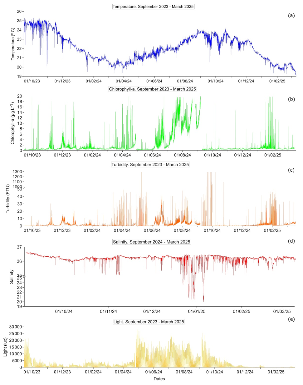
Figure 4 Annual measurements from 15 September 2023 to 10 March 2025: (a) temperature, (b) chlorophyll a, (c) turbidity, (d) salinity and (e) light intensity. The empty gaps in the chlorophyll a line represents the values above 20 µg L⁻¹ and negative values that were discarded. For the rest of the variables, the values are missing due to the maintenances in April and September 2024. The complete data set presented in monthly records is available in the Supplement.

3.1.3 Turbidity

Average monthly turbidity values ranged between 0.17 FTU (September 2023) and 25.19 FTU (September 2024) (Fig. 4C, Table S2 and Fig. S3 in the Supplement). The three highest monthly average values observed during the 18-month study period were in the spring of 2024 (April, 15.12 FTU) and in the autumn of 2025 (September, 25.19 FTU). Similar to chlorophyll a, the data set exhibited hourly peaks of high turbidity. For example, the turbidity peaks observed in April and September 2024. In contrast to other variables, there was not a clear seasonal pattern in turbidity concentration.

3.1.4 Salinity

Due to a failure in the conductivity sensor from September 2023 to September 2024, salinity was only recorded from 3 September 2024 to 10 March 2025. Salinity values presented in this section were on the practical salinity scale. Average salinity monthly values ranged between 34.84 (December 2024) to 36.38 (September 2024). The lowest average monthly values of the entire studied period were observed in December 2024 (34.84) (Fig. 4D, Table S1a in the Supplement), while the highest average monthly values were observed in September 2024 (36.38) (Fig. S4 in the Supplement).

3.1.5 Light

Light intensity pattern showed an evident diurnal variation. The seasonal light intensity of the summer 2024 and spring 2024 were almost 5 times higher than in the autumn 2023 and winter 2023 (Fig. S5 and Table S1a in the Supplement). Spring 2024 and summer 2024 showed the highest monthly average light intensity values of the entire record, especially during the period from end of April (Fig. 4E) to September 2024, when the maximum values were registered (between 19 445.76 and 28 323.84 lx). From November 2024 to March 2025, compared to the same period the previous year, monthly light intensity values were 2 to 14 times lower, probably affected by biological fouling over the sensor.

3.1.6 Dissolved O₂

The dissolved O₂ concentration was recorded only during three periods, September to October 2023 (45 d of data), April to May 2024 (17 d) and September 2024 to March 2025, due to a battery failure in the sensor (Fig. 5A to C). Average values for the first two periods were 8.95 and 9.60 mg L⁻¹, respectively (Table S1b in the Supplement). Average monthly values in the third period were between 9.19 and 9.93 mg L⁻¹ (Fig. S6 in the Supplement).

Dissolved O₂ showed adiurnal pattern with the highest daily values from afternoon to midnight. The diurnal variation between maximum and minimum values was less than 1 mg L⁻¹ daily difference on average in the September–October 2023, April–May 2024 and September–November 2024. However, the diurnal variation was more than 1.5 mg L⁻¹ daily difference between December 2024 and March 2025.

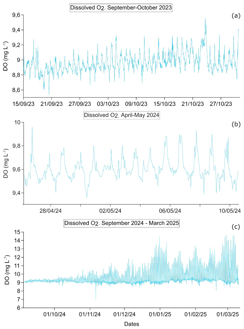
Figure 5 Dissolved oxygen measurements from 15 September to 30 October 2023 (a), from 26 April to 10 May 2024 (b) and from 3 September 2024 to 11 March 2025 (c). The complete data set presented in monthly records is available in the Supplement.

3.1.7 Current velocity and direction

Monthly average current velocity varied between 10.93 cm s⁻¹ (May 2024) and 17.80 cm s⁻¹ (October 2023) (Fig. 6A, Table S1b in the Supplement). A diurnal velocity variation was observed, suggesting a tidal pattern (Fig. 6B). There was no evident seasonal water current velocity pattern (details in Fig. S7 in the Supplement). The predominant water current direction was SE to NW, with alternating periods of NW to SE, (Fig. 6C, showing the example for October 2023 and Fig. 6D, for the period of September 2023 to April 2024, the entire record is in Fig. S8 in the Supplement). This water current direction pattern was observed during the entire study period. There was no data available between September 2024 to March 2025, due to a failure in the current meter.

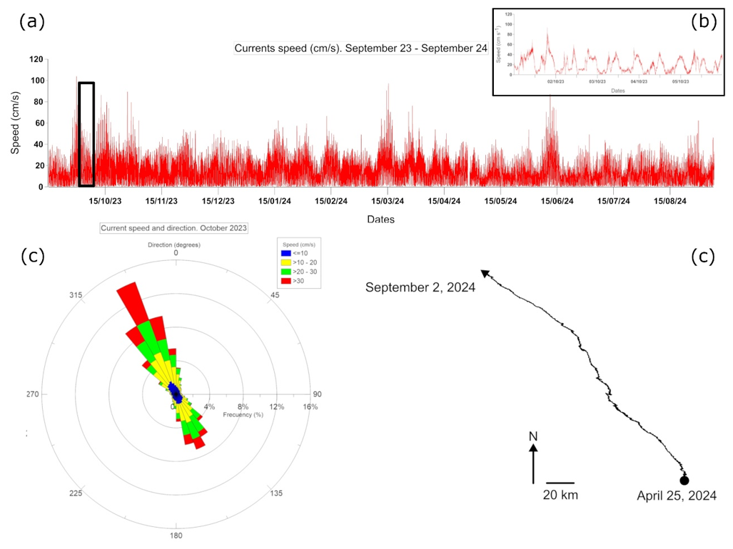
Figure 6 Annual current measurements and examples of current direction: (a) Current speed measurements from 15 September 2023 to 31 August 2024, (b) detail of a 5 d current speed (from 1 to 5 October 2025), (c) current speed and direction (degrees) for October 2023 and (d) polar vector plot, that describes the accumulative trajectory of a particle along the period between 15 September 2023 and 25 April 2024. The complete data set presented in monthly records is available in the Supplement.

3.2 Satellite observations

3.2.1 Chlorophyll

Based on satellite images, winter 2023 and winter 2024 were the seasons with the highest 8 d averaged chlorophyll values, both seasons with values that ranged from 0.2 to 0.5 mg L⁻¹ (weekly examples in Fig. 7A and full record in Fig. S9 in the Supplement). In contrast, spring 2024 showed the lowest 8 d averaged values, with a range from 0.05 mg L⁻¹ to 0.2 mg L⁻¹. Sea surface chlorophyll concentration showed a clear seasonal pattern, with the highest values during autumn and winter (0.2 to 0.5 mg L⁻¹) and the lowest in the spring (0.05 to 0.2 mg L⁻¹). The autumn 2023 showed the broadest variation in chlorophyll concentration along the study period (0.05 to 0.5 mg L⁻¹).

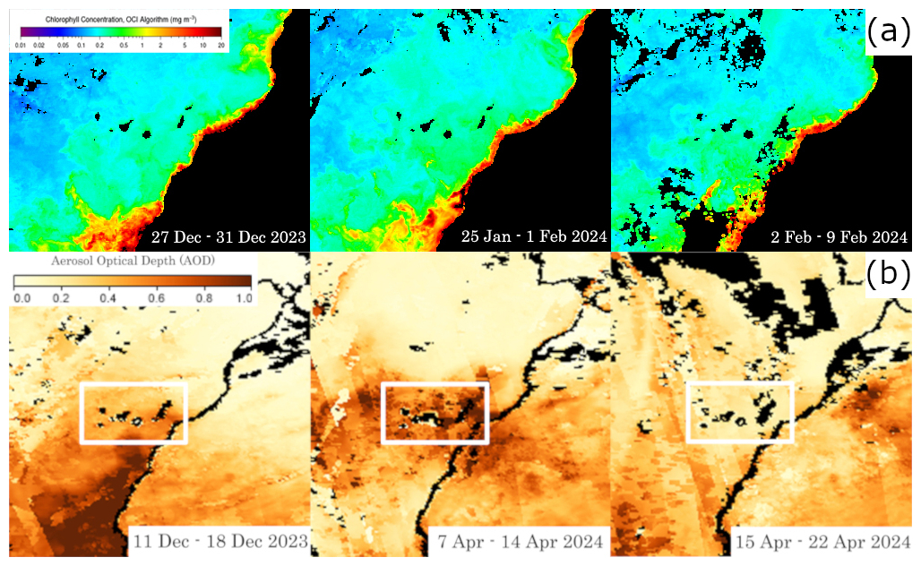
Figure 7 (A) satellite images showing the three weeks with the highest average chlorophyll concentration during the winter 2023–2024. (B) Satellite images showing three examples of weeks with highest AOD during the late autumn 2023 and spring and summer 2024. All images were provided by NASA Aqua MODIS satellite.

3.2.2 Aerosol Optical Depth

Aerosol Optical Depth (AOD) varied between 0.2 AOD and 0.7 AOD (weekly examples in Fig. 7B and full record in Figure S10 in the Supplement). The most intense calima activity took place during the summer of 2024. A period of six weeks with a practically uninterrupted AOD values between 0.3 and 0.7 developed from early July 2024 (Fig. 7B) until the end of August 2024. The highest values of the whole study period, 0.6 to 0.7 AOD, were observed in the second half of July 2024 and the second week of August 2024. The autumn 2023 and autumn and winter of 2024 showed the lowest calima intensity, with AOD values < 0.3, except for the third week of December, when AOD values reached 0.6.

3.3 Biomass

April 2024 biomass sample (BT₇) weighed 0.12 g, which made a total of 9.30 g for the entire sediment trap body area of 3.22 m² and a biomass per area value of 2.88 g m⁻² (Table 1). The September 2024 sample (BT₁₂) weighed 0.04 g, which equalled to 3.30 g and 1.02 g m⁻²after a year of development since T₀ (Table 1). The third sample (RT₁₂) collected in September 2024, weighed 0.08 g, representing a total of 6.51 g and 2.01 g m⁻² (Table 1). The fourth sample (BT₁₈) collected in March 2025, weighed 0.06 g that equals a total of 4.66 g and 1.44 g m⁻² (Table 1). Biomass results on T₁₂ and T₁₈ (BT₁₂, RT₁₂ and BT₁₈) were lower than T₇ most likely due to samples losses during collection (sample buoyancy and high current speed) and transport (plastic bag leakage during on-deck manipulation).

Table 1 Results from biomass and organic carbon (OC) are summarized in the following table.

3.4 Organic carbon

Organic carbon (OC) weighed 0.02, 0.01, 0.02 and 0.01 g for BT₇, BT₁₂, RT₁₂ and BT₁₈, respectively (Table 1) and represented a concentration in the biomass samples of 26.76 %, 23.38 %, 22.83 % and 14.53  % for BT₇, BT_12, RT₁₂ and BT₁₈, respectively. OC developed over the sediment trap body area was 1.58, 0.77, 1.47 and 0.67 g for BT₇, BT₁₂, RT₁₂ and BT₁₈, respectively (Table 1). These values corresponded to a production per area of 0.49, 0.24, 0.46 and 0.21 g C m⁻² for BT₇, BT₁₂, RT₁₂ and BT₁₈, respectively (Table 1). Due to the OC mass calculation was associated to the collected biomass, the results for BT₁₂, RT₁₂ and BT₁₈, were lower than BT₇.

3.5 Biodiversity and colonization

46 species belonging to 11 phyla were identified in the monitoring station and the nearest rock (Tables 2, 3, 4 and 5 and Fig. 8), corresponding to algae (7), sessile fauna (14), associated fauna (19) and pelagic fauna species (6). The primary producers Rhodophyta and Ochrophyta were the two most represented phyla in algae with 4 and 2 species, respectively. Cnidaria, Porifera, and Tunicata, were the four most represented phyla of sessile species with 7, 3, and 3 species, respectively. Chordata and Arthropoda, in the associated fauna, with 13 and 3 species, respectively, were the largest groups, whereas Chordata in the pelagic group stood out with 5 different species. The sessile species were mainly found on the fibreglass and concrete surfaces. The associated fauna species were found on the concrete and fibreglass surfaces and the natural rock. Pelagic species were only found more than 1 m away from the monitoring station.

Biomass coverage values (presence) ranged between 89.46 % in T₁₅ (December 2024) and 43.20 % in T₇ (April 2024) (Fig. 9). Absence (white-colored areas) was considered as grazed biomass based on the evidence of the observed dental scratching pattern on the fiberglass surface (Fig. 10A). Contrasting 100 % coverage values vs. the observed grazed (or no-grazed) areas (see Sect. 3.3 and 3.4, Table 1), it was possible to calculate the amount of biomass and OC transferred via trophic activity from the fiberglass surface. The biomass consumed was 13.29, 2.26, 5.11 and 1.55 g in April 2024 (BT₇), September 2024 (BT₁₂), September 2024 (RT₁₂), and March 2025 (BT₁₈) (Table 6), respectively. The OC transferred was 1.96, 0.44, 1.10 and 0.14 g in April 2024, September 2024 (BT₁₂), September 2024 (RT₁₂), and March 2025 (Table 6), respectively. The OC transferred per area was 0.61, 0.14, 0.34 and 0.04 g in April 2024, September 2024 (BT₁₂), September 2024 (RT₁₂), and March 2025 (Table 6), respectively.

Table 2 List of species identified in the monitoring station and surroundings. Species are classified by algae, sessile fauna, associated fauna and water column or passing by. Also, the surface where they were identified is marked by a cross.

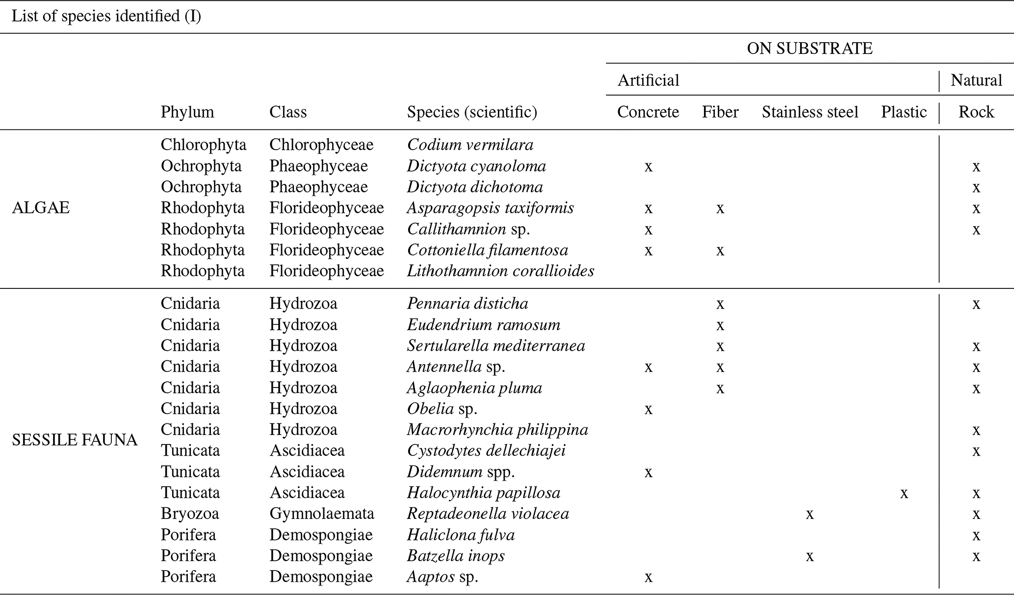
Table 3 List of species identified in the monitoring station and surroundings. Species are classified by algae, sessile fauna, associated fauna and water column or passing by. Also, the surface where they were identified is marked by a cross.

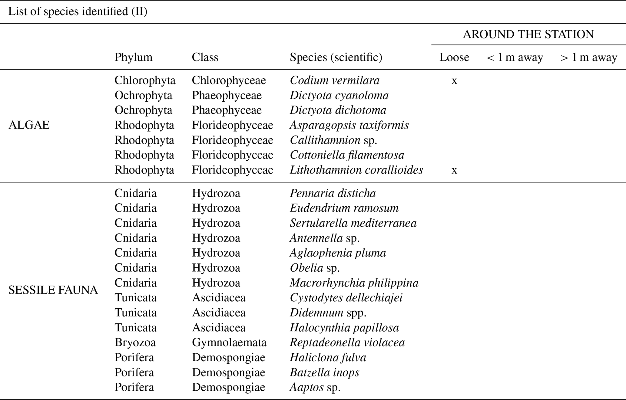
Table 4 List of species identified in the monitoring station and surroundings. Species are classified by algae, sessile fauna, associated fauna and water column or passing by. Also, the surface where they were identified is marked by a cross.

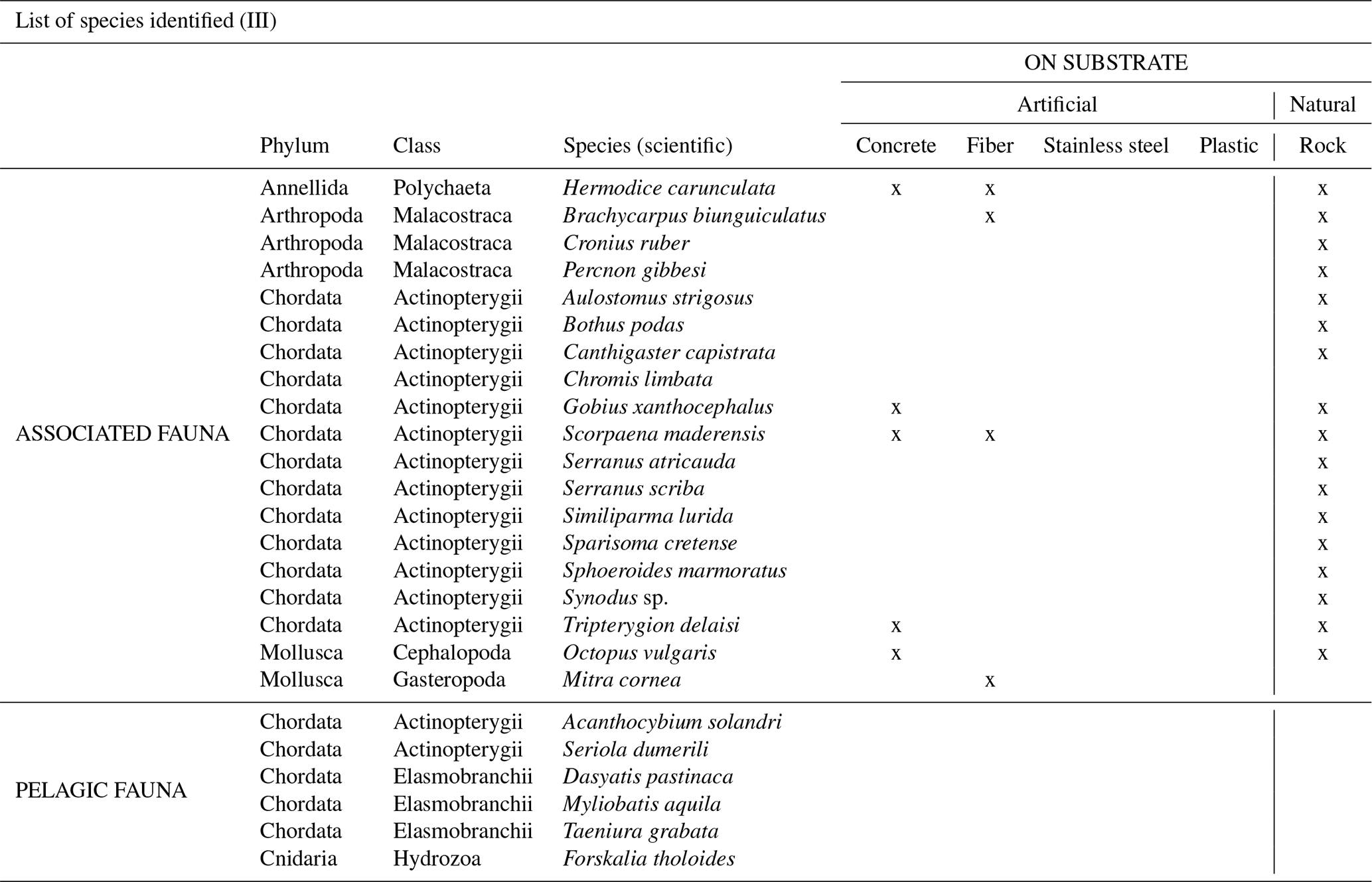
Table 5 List of species identified in the monitoring station and surroundings. Species are classified by algae, sessile fauna, associated fauna and water column or passing by. Also, the surface where they were identified is marked by a cross.

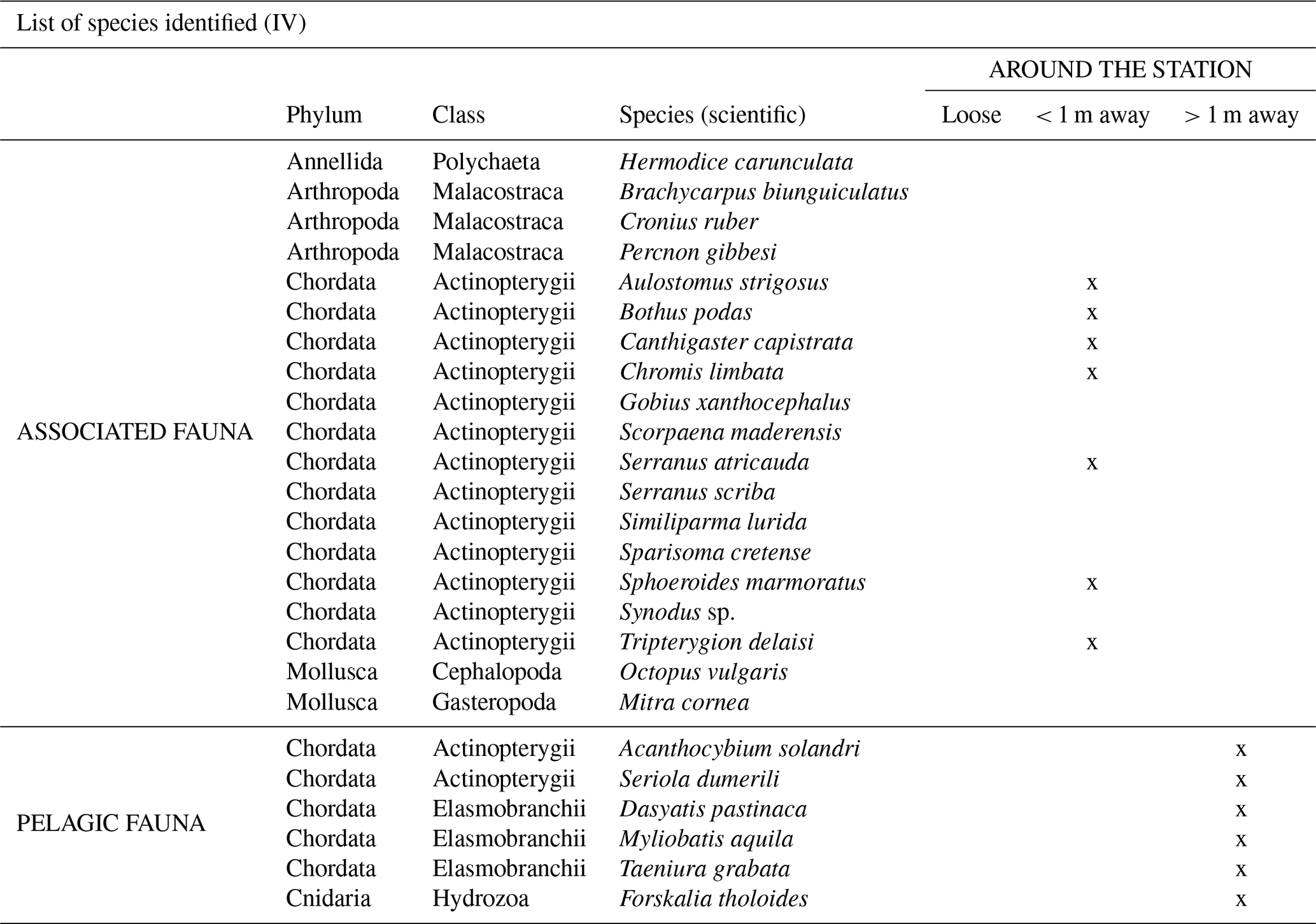
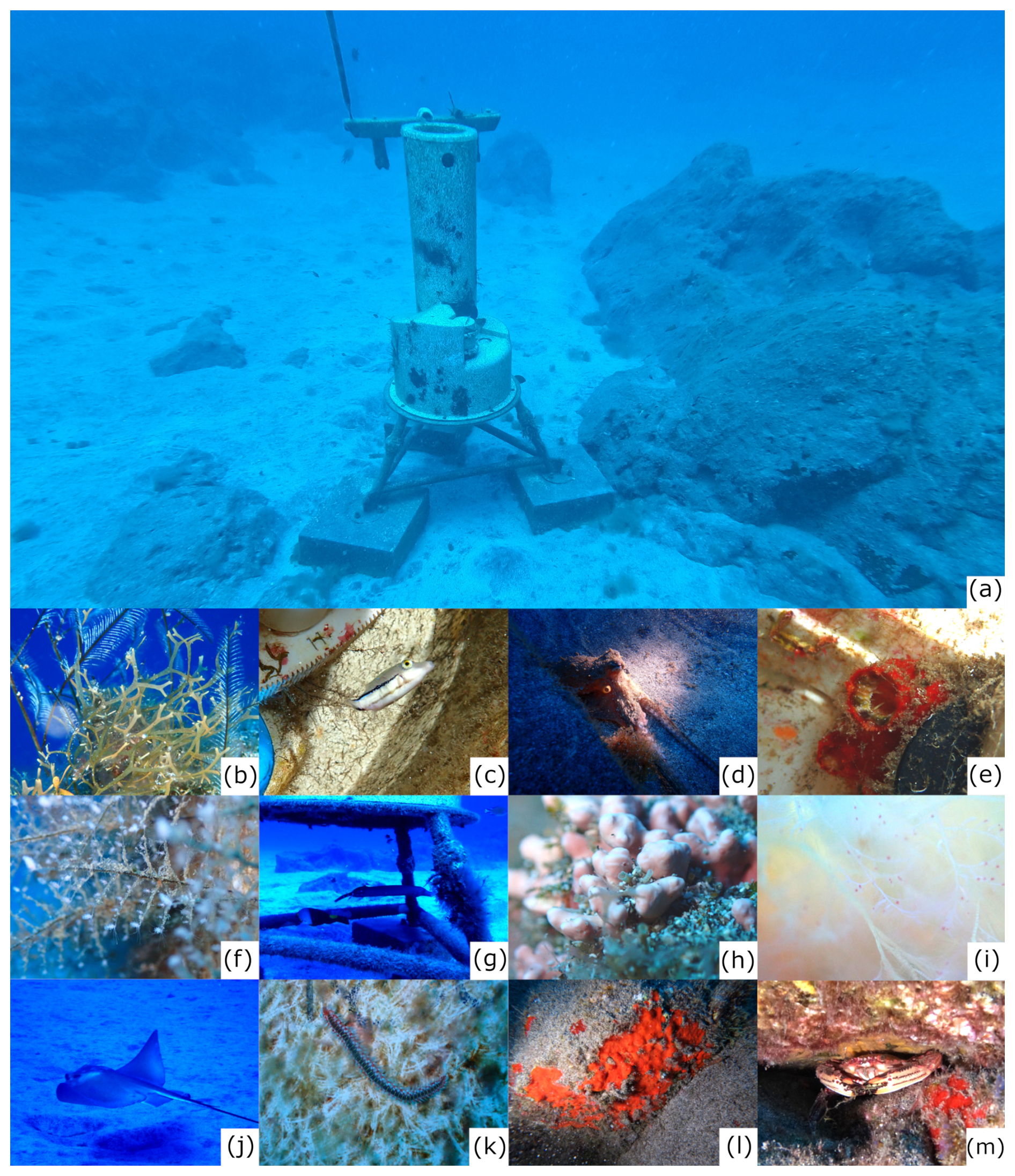
Figure 8 (a) position of the monitoring station and the nearest rock where organisms were identified. Examples of some organisms identified in the different dives. (b) Top (Macrorhynchia philippina) and below (Dictyota cyalonoma), (c) Canthigaster capistrata, (d) Octopus vulgaris, (e) Halocynthia papillosa, (f)  Pennaria disticha, (g) Aulostomus strigosus, (h) Lithothamnion corallioides, (i) Cottoniela filamentosa, (j) Myliobatis aquila, (k) Hermodice carunculata, (l) Batzella inops, (m) Cronius ruber. Photos by: Isabelle Peeters.

Table 6 Calculations of the biomass and organic carbon that would have been generated without the grazing action. Calculations were made combining the coverage data obtained and the biomass collected in April 2024, September 2024 and March 2025.

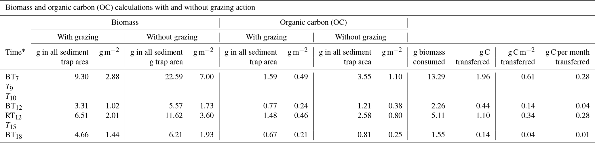
^* BT₇ (April 2024), T₉ (June 2024), T₁₀ (July 2024), BT₁₂ and RT₁₂ (September 2024), T₁₅ (December 2024) and BT₁₈ (March 2025).

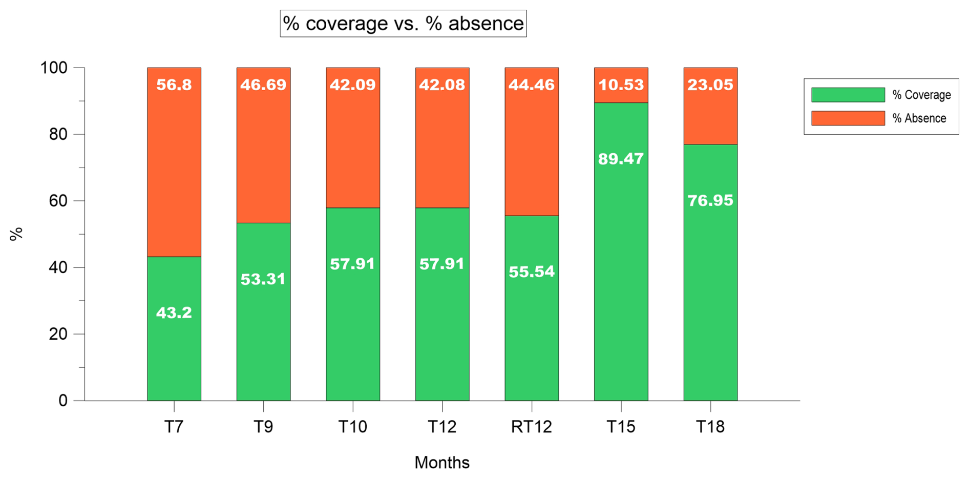
Figure 9 Evolution of the % of coverage/absence of colonization during the monitored period. T₇ (April 2024), T₉ (June 2024), T₁₀ (July 2024), T₁₂ and RT₁₂ (September 2024), T₁₅ (December 2024) and T₁₈ (March 2025).

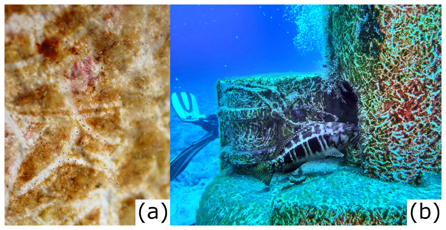
Figure 10 (A) detail of grazing marks produced in the fiberglass surface. White marks represent the grazed area. (B) a fish (Serranus atricauda) grazing the station surface. Photos by: Isabelle Peeters.

3.6 Estimations of biomass loss during collection

Sample loss could have occurred during the collection of BT₁₂, RT₁₂ and BT₁₈. Here we estimate, based on BT₇ values, the amount of biomass and the associated OC that would have been produced during the entire period of the study. Based on the results on biomass coverage presented in Sect. 3.5, it was estimated that the amount of biomass developed in T₁₂ and T₁₈ (i.e. BT₁₂, RT₁₂ and BT₁₈) without any loss during sample collection, was expected to be greater than the values reported in Table 1. The biomass coverage in BT₁₂, RT₁₂, BT₁₈ was 14.71 %, 12.34 % and 33.75 % greater than in T₇ (Fig. 9), respectively. Considering the collected biomass at T₇ as a maximum value, e.g., no visual evidence of biomass loss, and using the biomass sampled with the 20 cm × 20 cm square in T₇ (0.12 g) and the coverage in T₇ (43.2 %), the expected biomass per square in BT₁₂, RT₁₂ and BT₁₈ was estimated based on the coverage values reported in Fig. 9. Assuming a linear biomass growth, the estimated biomass values were 0.16, 0.15 and 0.21 g, respectively (Table 7). The estimation of the biomass produced over the sediment trap area would be 12.91, 12.10 and 16.94 g for BT₁₂, RT₁₂, and BT₁₈, respectively (Table 7). The estimation of the biomass per area would be 4.00, 3.75 and 5.25 g m⁻² for for BT₁₂, RT₁₂, and BT₁₈, respectively (Table 7).

In the same way, the full amount of OC, that would have been produced, was estimated (Table 7). The estimations of OC produced per 20 cm × 20 cm square would be 0.04, 0.03 and 0.03 g for BT₁₂, RT₁₂, and BT₁₈, respectively. The OC developed over the sediment trap area would be 2.90, 2.71 and 2.31 g C for BT₁₂, RT₁₂, and BT₁₈, respectively. The estimation of OC developed per area would be 0.90, 0.84 and 0.72 g C m⁻² for BT₁₂, RT₁₂, and BT₁₈, respectively.

Based on the results presented above, the estimated amount of biomass and OC, assuming no sampling losses, relative to the values reported in Sect. 3.3 and 3.4. (Table 1), would have been at least three-fold, two-fold and approximately 2.5-fold higher for BT₁₂, RT₁₂ and BT₁₈, respectively.

Table 7 Estimation of biomass and OC without sampling losses. BT₇ row values are used as a reference.

3.7 Statistical methods

Two pairs of variables were used to apply the Spearman test, current speed vs. turbidity and chlorophyll a vs. turbidity. These pairs of variables were selected to test the statistical relationship between them, because these variables are likely to be strongly related to each other. For example, sediment resuspension may increase with higher current velocities, whereas the increase in chlorophyll a abundance is related to the increase of pigment bearing particles. The Spearman test for the current speed and turbidity produced Spearman's rank correlation coefficient ρ (rho) of −0.014 (Table S3 in the Supplement), indicating the absence of significant association. Spearman correlation analysis revealed a strong association between chlorophyll a and turbidity throughout the study period. Considering the entire dataset (September 2023–March 2025), the correlation coefficient was high (ρ=0.761) (Table S3 in the Supplement). Seasonal correlation coefficients ranged from 0.416 in autumn 2024 to 0.875 in autumn 2023. The strongest associations were observed in autumn 2023 (ρ=0.875) and spring 2024 (ρ=0.815), whereas the weakest correlations occurred in autumn 2024 (ρ=0.416) and winter 2024 (ρ=0.546). Despite this seasonal variability, no clear seasonal or interannual trend emerged. Similar correlation coefficients were observed during winter 2024 and winter 2025 (ρ=0.546 and 0.561, respectively), contrasting with the marked differences between autumn 2023 and autumn 2024 (ρ=0.875 and 0.416, respectively).

Regarding the correlation between chlorophyll a and turbidity after a calima event, the correlation was very strong in April 2024 and December 2024 (ρ=0.892 and ρ=0.884, respectively), while in the case of July 2024, the correlation was very weak (ρ=0.368) (Table S4 in the Supplement).

3.8 Ecosystem Services

The results on the identified ecosystem services and its indicators are shown in Table 8. The combination of the CICES method and the indicators derived from the data obtained in this study permitted the identification of five ecosystem services. These were identified and classified eighteen months after the installation of the monitoring station. It was found that one ecosystem service corresponded to the provisioning category (e.g., primary production), three to regulation and maintenance (e.g., nursery habitat, refuge or shelter, biodiversity maintenance and climate regulation) and one to cultural category (e.g., knowledge). The following indicators permitted the identification of the ecosystem services: (1) the amount of benthic biomass grown (e.g., total mass of biomass (g) and its spatial abundance (g m⁻² biomass) over time) over the monitoring station along the study period was used to identify primary production, (2) the identification of fish juveniles around the monitoring station and the presence of organisms using the monitoring station as a refuge (e.g., Canthigaster capistrata, Octopus vulgaris, Scorpaena maderensis or Chromis limbata, among others) for the identification of nursery habitat, refuge or shelter, (3) the number of different species found during the periodic monitoring dives (46 species belonging to 11 phyla) was used as indicator of biodiversity maintenance, (4) the amount of organic carbon retained on the surface of the installation (e.g., g C and g C m⁻²) was used to identify climate regulation and (5) the generated data set and the findings that provide information for the publication of scientific studies, reports and dissemination as the indicator of knowledge (development).

Table 8 Results from CICES method application for ecosystem services identification and classification. The results from the literature search about ecosystem services name and the indicators used in this work are included for each ecosystem services.

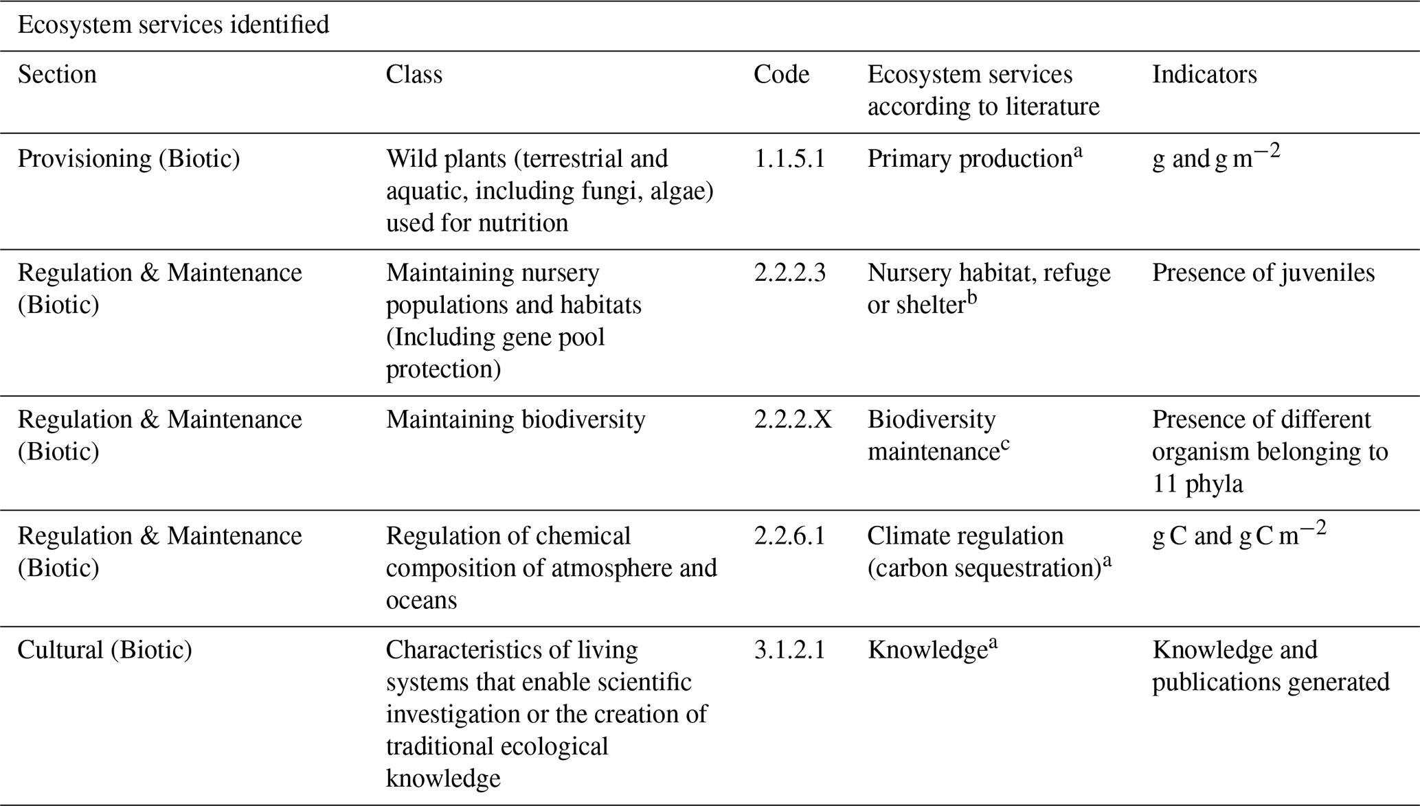
^a Millenium Ecosystem Assessment (2005), ^b Liquete et al. (2016), ^c Haines-Young and Potschin (2018).

4 Discussion

Information on the physical and biological characteristics at the shallow coastal fringe off Tenerife and the Canary Island Archipelago is scarce (Valdés and Déniz-González, 2015). In contrast, biodiversity abundance and composition of pelagic and benthic fauna in the area is better known (Afonso-Carrillo et al., 2007; González et al., 2025; Moreno-Borges et al., 2024). Further, the information on ecosystem services on Canary Island waters is poor (Cordero-Penín et al., 2023) and no information exists on blue carbon development in the study area. Therefore, this study represents the first of its kind for this area of the Canary Islands.

The present study provides important observations on an anthropogenic installation (e.g., submarine monitoring station) that functioned as an unintentional artificial reef and enabled the assessment of blue carbon development and the feasibility that restoration efforts may have in the shallow coastal fringe in oligotrophic areas (e.g., without riverine nutrient inputs), including the provision of ecosystem services and the quantification of the observed biodiversity associated to this structure.

4.1 Physical variables

In Canary Island waters, the sea surface temperatures (SST) usually range between 17 °C in winter to 25 °C in summer (Clemente et al., 2011; Ramos et al., 2008). However, in some areas to the south of the Canary Islands, SST presented unprecedented peaks of 28.5 °C during summer in 2004 (Ramos et al., 2005). The results obtained in the present study at the station site were in the expected range for Canary Island waters (Fig. 4A), in spite of the fact that 2024 has been one of the warmest years on record, with an average > 1.5 °C above the pre-industrial period values (https://wmo.int/news/media-centre/wmo-confirms-2024-warmest-year-record-about-155degc-above-pre-industrial-level, last access: 29 October 2026). The monthly average salinity values measured between September 2024 and March 2025 were between 34.84 and 36.38 (Fig. 4D). Some studies on Canary Island surface waters report higher salinity values (e.g., 36.5 to 36.8) (González-Dávila et al., 2003; Hernández-Guerra et al., 2000) than those measured in this study. Based on the shallow location of the monitoring station in the water column (e.g., 25.5 m water depth) the water mass affecting the studied site is surface water (Casanova-Masjoan et al., 2020; Pastor et al., 2008). Surface water is characterized by the high temperature and salinity variation due to seasonal heating, evaporation, precipitation, influence from the upwelling or upwelling filaments, wind mixing and local atmospheric conditions (Casanova-Masjoan et al., 2020; González-Dávila et al., 2003; Knoll et al., 2002). The salinity dropped between the late December 2024 and early January 2025, when average monthly values were the lowest of the entire record. The evident salinity decline between December 2024 and January 2025 (Fig. S4 in the Supplement) was not associated with precipitation, based on the AEMET monthly reports (https://www.aemet.es/es/serviciosclimaticos/vigilancia_clima/resumenes, last access: 27 March 2025), which indicated that December 2024 and January 2025, were dry and within normal values.

The comparatively low average (e.g., < 36) and the various irregular discontinuous drops (e.g., < 35.5) in the salinity record (Fig. 4D), strongly suggest that the observed pattern could represent the effect of uncontrolled underwater sewage discharge by the submarine outfalls near the station (Fig. S11 in the Supplement). These outfalls discharge at 22 and 24 m water depth; thus, the discharge dilutes before reaching the station's site and the effect over the station's CTD sensor may only affect slightly the salinity, which is enough to make salinity lower than 35.5. Based on the water current speed record (Fig. 6), particles coming from these outfalls can reach the station in periods between 56 and 167 min.

In the present study, average turbidity values were relatively low (e.g., 5.47 FTU of average on the study period). Current speed and direction were not significantly related to turbidity and cannot explain the turbidity pattern (Table S3 in the Supplement). A semi-diurnal tidal pattern was detected in the current velocity data (Figs. 6B, S7 in the Supplement); however, this pattern was not evident in the turbidity data (Figs. 4C, S3 in the Supplement), suggesting that sediment resuspension due to tidal currents was not the main factor responsible for the observed turbidity pattern. During April 2024 and May 2024, there were various high-turbidity episodes, coinciding with chlorophyll a peaks, suggesting that high turbidity could also be caused by irregular atmospheric dust deposition (e.g., AOD values between 0.2 and 0.5, Fig. S10a and b in the Supplement) in combination with episodes of organic matter dumping by the underwater outfall near the station and the consequent presence of chlorophyll a-rich particles.

In the Canary region, from 20 to 26° N, light intensity is high, especially in the central cloud-free desert region, with quasi-permanent trade winds. However, light intensity is lower in the study area (located at 28° N), with a light intensity maximum in summer (Demarcq and Somoue, 2015; Gómez-Letona et al., 2017). The observed annual light intensity pattern at 25.5 m water depth also showed a summer maximum, aligned with the annual pattern observed to the North of the present study area (Demarcq and Somoue, 2015) (Figs. 4E, S5 in the Supplement). There are no studies on light intensity measured in Lux near the Canary Islands waters, the available PAR (Photosynthetically active radiation) data collected at 20 m water depth to the North of the Canarian Archipelago suggest that values measured at the study site were within the typical parameter (Lux = PAR ×60) for Canary Islands waters (Zielinski et al., 2002).

The average dissolved O₂ results, between 8.95 and 9.93 mg L⁻¹, indicated that the submarine station was installed in a well-oxygenated environment (Webb, 2019; Fondriest Environmental, 2013), most likely due to the action of waves and wind mixing over a relatively short water column.

The observed physical environmental conditions at the submarine station indicated that the study site shows no oxygen, light, temperature and/or chlorophyll limitations for benthic biomass development. Thus, the conditions at the study site are beneficial for blue carbon development, stimulated by natural fertilization caused by calima and upwelling events in addition to anthropogenic inputs from sewage discharges. Further, the water current pattern suggests that these conditions could be similar along the SW coastline of Tenerife (approx. 70 km long).

4.2 Biological variables

According to the classification of Håkanson and Bryhn (2008) and Purnamaningtyas and Mujiyanto (2021), the waters in the study area were generally oligotrophic (Chl a < 2 µg L⁻¹). During 16 months from September 2023 to May 2024 and from September to March 2024 waters in the study area were oligotrophic, during June 2024 mesotrophic (Chl a 2 to 6 µg L⁻¹) and during July and August 2024 they were eutrophic (Chl a between 6 and 20 µg L⁻¹). Abrupt and isolated chlorophyll a concentration peaks were observed along the study period; these anomalous increases could be related to sensor malfunctions and/or discharges from the two underwater outfalls located 1 km to the northwest and 1 km southeast of the station (Fig. S11 in the Supplement). The main current direction flows parallel to the coast line, from SE to NW (Figs. 6C, S8 in the Supplement); consequently, it is likely that submarine outfall discharges, phytoplankton blooms, suspended sediments, dissolved nutrients, etc., coming from the SE affected the station site. Periods of water current flowing from the SE to the NW with > 30 cm s⁻¹ were observed, implying that unauthorised underwater outfall discharges could reach the submarine station within ∼ 55 min (Fig. 6D). Water current periods with direction NW to SE were less frequent and less intense (mainly with < 30 cm s⁻¹ speed). Nevertheless, unauthorised underwater outfall discharges to the NW could also reach the submarine station during NW to SE water current events longer than 1 h. Data showed that the occurrence of chlorophyll a peaks was independent of the current direction. This suggest that the underwater outfall discharges alone cannot explain the chlorophyll a pattern. The observed chlorophyll a peaks could also be influenced by entrainment of high-chlorophyll water originating over the island's continental shelf or the African coastal upwelling (Arístegui et al., 1997). According to Barton et al. (1998), the annual primary production cycle in Canary Islands' waters unaffected by the NW African coastal upwelling is divided in three periods: (1) late winter bloom, when seasonal thermocline is eroded and nutrients from deeper layers are mixed up into surface waters (2) summer season, when the highest annual trade winds intensity generates high local coastal upwelling activity and (3) the autumn season, when plankton productivity falls to its lowest annual values. During the present investigation, the highest chlorophyll a concentration corresponded also to the summer and the lowest to the autumn, coinciding with the annual pattern of upwelling and primary production periods observed for the region (Table S2 in the Supplement). However, our data showed that the late winter bloom observed by Barton et al. (1998), took place between late autumn and early winter in the shallow near-shore environment to the south of Tenerife, perhaps showing a different pattern in the near-shore environment relative to off-shore waters or simply showing interannual variation (cf. Barton et al., 1998). This temporal-spatial mismatch could also be due to the intrusion of chlorophyll a-rich filaments detached from the NW African coast (e.g., Cape Juby (Morocco) and Cape Bojador (Western Sahara)), towards the study area (Arístegui et al., 2009; Barton et al., 1998; Siemer et al., 2021). These filaments at Cape Juby and between Cape Juby and Cape Bojador are small, intermittent and special variability due to their interaction with an eddy field induced by the Canary Islands; thus, potentially able to introduce irregular and chlorophyll a rich signals into the study area (Barton et al., 1998, 2004).

Satellite imagery was used to identify or discard between regional (e.g., upwelling or calima) and local events (e.g., underwater sewage discharges) affecting the study area despite the fact that measurements obtained from the monitoring station and from satellite differ in some factors. Those factors were sensor resolution (single point resolution of 1 m vs. 4 km resolution, respectively), temporal resolution (hourly measurement vs. 8 d average, respectively), measurement units (µg L⁻¹ vs. mg m⁻³) and water depth (25.5 m water depth vs. surface layer of ∼ 5 m water depth).

Remote and in situ chlorophyll concentration measurements showed similar patterns from September 2023 to March 2024 and May 2024. Different patterns were observed from April to September 2024 (excluding May), when the chlorophyll a measured at the monitoring station was comparatively high relative to the study period (Table S2 in the Supplement). Conversely, the chlorophyll concentration measured by satellite showed comparatively low values (Fig. S9 in the Supplement). This discrepancy could be attributed to the presence of local phytoplankton blooms, probably induced by the underwater sewage discharge from submarine outfalls near the station. These blooms were not remotely detected due to the limited spatial resolution of satellite data. In contrast, from September 2024 to March 2025, the chlorophyll concentration measured by the satellite was high in relative to the chlorophyll a concentration at the monitoring station. The quasi-permanent low-intensity calima which fertilised ocean surface waters during the late summer 2024, autumn 2024 and early-winter 2024 (Fig. S10c in the Supplement), and the stratification of the water column during this period (Schmoker and Hernández-León, 2013), which prevented water mixing, were likely the main factors behind these discrepancies in chlorophyll concentration.

According to NASA (https://neo.gsfc.nasa.gov/view.php?datasetId=MYDAL2_E_AER_OD&date=2023-12-01, last access: 27 March 2025), AOD < 0.1 indicates a crystal-clear sky with maximum visibility, whereas AOD values > 1 indicates the presence of aerosols, so dense that people would have difficulty seeing the Sun, even at mid-day. Calima recurrence is higher in winter (Dorta et al., 2005; Suárez-Molina et al., 2024), whereas from April to June the recurrence is the lowest according to Gelado et al. (2003). The dust intensity over the submarine station in the present study could be classified as low to medium during autumn and winter, with AOD indexes of 0.2 to 0.5 and one event in April 2024 as medium to high, with AOD values ∼ 0.6 (Fig. 7B). AOD obtained from satellite imagery during the study period (e.g., September 2023–March 2025), showed comparatively high values and frequent events in winter and less intense and frequent events in autumn and spring, coinciding with the seasonality of African dust presence, particularly in winter. However, contrary to Gelado et al. (2003) the highest AOD levels during the study period in 2024 were observed during an extraordinary event in April, followed by a strong and persistent calima in the summer season (Fig. S10 in the Supplement). Following the strong calima in April 2024, extraordinary high levels of turbidity and chlorophyll a concentration were measured at the submarine station (i.e. from 7 to 24 April) (Fig. S12 in the Supplement). A similar relationship was observed during the second and third week of December 2023, when after a calima event, both variables increased reaching the highest values of the month (Fig. S13 in the Supplement). Following the persistent summer calima (from the second week of July 2024 until the second week of August 2024), there were extraordinarily high levels of chlorophyll a measured at the submarine station in July and August 2024 (Fig. S14 in the Supplement). The temporal coincidences among calima, chlorophyll a and turbidity observed at the submarine station (e.g., April and December 2024), suggest that calima could be related to the increase in chlorophyll a at 25.5 m depth, corroborating the well-known fertilization effect of Saharan dust deposition over the ocean (Franchy et al., 2013; Ramos et al., 2008). A common characteristic among the April 2024, July 2024 and December 2023 events (Figs. S12, S13 and S14 in the Supplement) was a 2 to 5 d delay between the end of the calima period and the maximum chlorophyll a concentration measured by the monitoring station at 25.5 m depth. The time-lag effects on chlorophyll a and turbidity following the calima events of April and December 2024 were supported by a very strong correlation among these parameters (Table S4 in the Supplement). In contrast, only a weak correlation between chlorophyll a and turbidity was observed following the July 2024 calima event (Table S4 in the Supplement). Unlike the April and December events, the elevated chlorophyll a concentrations recorded in July were not accompanied by a comparable increase in turbidity. This discrepancy suggests that phytoplankton biomass was likely influenced by local nutrient sources, such as underwater sewage discharges, rather than solely by the fertilising effects associated with calima deposition. Nevertheless, it cannot be ruled out that the high chlorophyll a concentrations resulted from the combined influence of calima-derived nutrient inputs and a significant underwater sewage discharge. This 2-to-5 d time span among observations may provide information on the phytoplankton response time to calima-induced fertilization in near-shore environments.

The light sensor recorded low intensity values on days with calima. For example, the strong and persistent calima in summer 2024 and specially in August, was clearly noticeable in the light intensity record (Fig. S15 in the Supplement) showing that light intensity measured at 25.5 m water depth was lower in days with calima than in periods without calima. As example of light intensity attenuation, we compared the 2nd week of June 2024 (from 12 to 19 June), which was a week without calima, with a week with strong calima, the 3rd week of August 2024 (from 13 to 20 August). The 3rd week of August mean daily light intensity attenuation was 19.68 % (Fig. S15 in the Supplement). Visible light attenuation due to calima may contribute explaining the temporal delay in the phytoplankton response time after the calima fertilization of the water column. Biofouling may also attenuate the light intensity reaching the sensor. Two light-attenuation periods were observed from the end of October 2024 to March 2025 and from November 2024 and March 2025. The light intensity was extraordinarily low compared to the period from November 2023 to March 2024 (Fig. S5 in the Supplement). During March 2025 maintenance operations, it was observed that light intensity sensor was covered by biofouling. The light intensity records suggested that the light intensity sensor was rapidly colonized in two months following the September 2024 maintenance operations, perhaps stimulated by the summer calima events (e.g., August 2024). Biofouling on the light sensor provides qualitative evidence to demonstrate and estimate the benthic biomass production pace at the study site.

Satellite observations confirmed in situ measurements, which showed that chlorophyll a abundance in the water column was not a limiting factor for secondary production and accompanied benthic biomass development on the fiberglass submarine station's body, at least from September 2023 to March 2025. The combination AOD variation with chlorophyll a in-situ measurements suggests that chlorophyll a abundance is influenced by African dust deposition. Based on the available information, the observed temporal variation for chlorophyll a abundance at 25.5 water depth seems to be the result of a combination of factors both, remote (e.g. Saharan dust and upwelling events off the African coast) and local (wind-induced upwelling, submarine outfall discharges), which together developed no temporal (or seasonal) pattern.

4.3 Ecosystem services

4.3.1 Benthic biomass and organic carbon development

Similar to cases of lost fishing gear (Villafranca-Sánchez et al., 2025) and moorings (Castellan et al., 2026), the monitoring station in the present study functioned as an unintentional artificial reef. This situation provided the opportunity to assess the biomass growth and quantify the amount of organic carbon produced during the study period. However, the results presented here must be interpreted with some caution as sampling relied on a single, non-replicated installation and the sampling conditions itself (e.g., lightness of the samples and water current velocity during SCUBA diving manoeuvres). Therefore, the results on biomass weight and carbon content represent the lowest possible values due to losses during sample collection and handling (see the Methods section). Although the biomass loss estimations in Sect. 3.7 were calculated assuming a linear increase in biomass and no sampling losses, biomass (e.g. biofilm) growth is known to follow a non-linear pattern, with a rapid initial colonization followed by a progressive maturation and stabilization (Sauer et al., 2022). Consequently, while the linear approach provides a practical approximation of biomass and OC development, it may oversimplify the growth dynamics. However, there is no information on blue carbon development in the area to compare with the present results. This study is the first of its class for the SW coast of Tenerife, therefore the values reported here can be used as a potential baseline for future assessments on blue carbon development and benthic restoration efforts. On the study site, biofouling on the light intensity sensor and the light attenuation pattern showed intense blue carbon (e.g., benthic coverage) developing in only two months. The OC calculated here represents the remaining OC after the transfer of biomass to higher levels in the food web based on the omnipresent grazing marks over the entire monitoring station surface and during the 18-month study period (Fig. 10A). These marks are consistent with the activity of associated species like Serranus atricauda (Tables 4, 5 and Fig. 10), which was frequently observed in close proximity (< 1 m) to the station, likely contributing to biomass removal while foraging for microfauna within the biofilm. Based on the grazing marks observed, comparing the results obtained in BT₇ (1.59 g C), BT₁₂ (0.77 g C), RT₁₂ (1.48 g C) and BT₁₈ (0.67 g C) and analysing the biomass coverage in the various observations (43.20 %, 57.92 %, 55.54 % and 76.95 % for T₇, T₁₂, RT₁₂ and T₁₈, respectively), it can be assumed that the carbon generated by the monitoring station reached a biomass development, consumption and regeneration steady state in about seven months. This steady state was maintained between April (T₇) until September 2024 (T₁₂) (Fig. 9). However, from September 2024 (T₁₂) to December 2024 (T₁₅), an increment of colonization was observed. In December 2024 (T₁₅), coverage of the fiberglass surface analysed was 89.47 %. The increase between September and December is difficult to interpret with the available information; the environmental conditions at the submarine station did not show an abrupt variation that could explain extraordinary benthic growth or pelagic migrations (e.g., decrease in consumption). In the same way, there was a slight blue carbon biomass decrease between December 2024 and March 2025, although environmental conditions did not show any variations that could explain the change in biomass consumption. However, alterations in the grazer's life cycle or displacement of the grazing individuals should not be discarded. In any case, the available photographic evidence showed that grazing is a main factor regulating blue carbon persistence at the study site, implying that between 11 % and 57 % of the blue carbon generated there was transferred to upper levels in the food web (Fig. 9). These percentages represented blue carbon masses between 0.04 g C m⁻² (BT₁₈) and 0.61 g C m⁻² (BT₇) (Table 6).

Seagrass meadows, salt marshes and mangroves are the most important blue carbon ecosystems immobilizing carbon. Seagrass carbon burial capacity is equivalent to 83 grams of carbon per square meter per year (g C m⁻² yr⁻¹) (CCA, 2016). Salt marshes with a global distribution display a carbon burial rate of 218 ± 24 g C m⁻² yr⁻¹ (McLeod et al., 2011). The carbon burial rate in mangroves is 226 ± 39 g C m⁻² yr⁻¹ (McLeod et al., 2011). Gorgonians (soft corals) are important marine animal forest engineers (Coppari et al., 2019) that provide substrate for macrobenthic fauna to thrive and structure for blue carbon development. In the NW Mediterranean, three gorgonian species (Paramuricea clavata, Eunicella singularis, Leptogorgia sarmentosa) sequestered respectively, 0.258, 0.890 and 0.002 g C m⁻² yr⁻¹ by growth (Coppari et al., 2019). These values did not consider associated species such as sponges, bryozoans, coralline algae, among others, which also sequester carbon due to the presence of gorgonians (Coppari et al., 2019). The carbon sequestration rate in oligotrophic benthic ecosystems like coralline assemblages and rhodoliths beds is 330 g C m⁻² yr⁻¹ (van der Heijden and Kamenos, 2015) and 19 g C m⁻² yr⁻¹ (Rossi, 2022), respectively. In high latitude, for example, the Burdwood Bank in the Southern Ocean, benthic assemblages showed a carbon content of 0.8 g m⁻². Further into the south, in the Bellingshausen Sea, the western Ross Sea shelf and the continental shelves at South Georgia, South Orkneys Islands and the Weddell Sea, the macrobenthic faunal carbon content was 0.7, 0.68, 0.17, 2 and 1 g m⁻², respectively (Bergagna et al., 2024). These comparisons show that the oligotrophic shallow environment off the SW coast of Tenerife, which generates 0.24 g C m⁻² yr⁻¹ (0.38 g C m⁻² yr⁻¹ without grazing) (Table 6) would be among the benthic ecosystems with the lowest global blue carbon production levels. Nevertheless, the environmental conditions at the southern coast of Tenerife seem able to maintain a sustained blue carbon production-and-transfer ecosystem that, with the introduction of artificial reefs, may favour the maintenance of the local biodiversity pool, contributing further for the provision of ecosystem services.

4.3.2 Biodiversity

46 species belonging to 11 different phyla were identified living in the vicinity and on the different materials composing the submarine station (Tables 2, 3, 4 and 5). This community included primary producers such as Cottoniela filamentosa (Rhodophyta), sessile suspension feeders such as Pennaria disticha (Hydrozoa) and motile species such as Hermodice carunculata (Polychaeta) (Fig. 8b–m). The assemblage of this community indicates that the monitoring station is contributing to the maintenance of the local marine biodiversity, providing food (e.g., energy), refuge and nursery grounds, generating additional supporting ecosystem services (Fig. 11). The present study censed the species present on the artificial structure and verified their presence on the neighbouring natural substrate as well. The observations made on the artificial structure were categorised per type of material (e.g., concrete, fiberglass and stainless steel). The artificial structure showed lower algae abundance than on the natural rock in terms of biodiversity (4 vs. 5 species, respectively) (Table 2). As for fauna, 9 species (5 sessile and 4 associated) were observed on the fiberglass surface, whereas 27 species (10 sessile and 17 associated) were observed on the neighbouring rock. Here, it should be considered that the fiberglass is a homogeneous, artificial, non-porous surface, unintentionally working as substrate, which may favour the settlement of some species over others. Therefore, the potential of the sediment trap body for sessile benthic species to thrive is small relative to a rock, where more diverse substrate characteristics occur (e.g., light availability, porosity, steepness, water current protection, etc.). The presence of grazers (e.g., Actinopterygii) living on the natural rock and around the monitoring station (Table 5) was higher in the natural rock than around the station (12 vs. 7 species identified, respectively). In the case of filter feeding organisms (e.g., Porifera, Tunicate and Bryozoa) the number of species identified living in both habitats was the same (5 species). McKibbin et al. (2024) observed for coastal infrastructures such as seawalls, breakwaters or artificial reefs that less habitat-forming algae were present relative to a natural habitat, where filter feeding organisms were more abundant than grazers. However, to the south of Tenerife, we found a similar presence of grazers and filter feeding organisms thriving on both the fiberglass and the natural substrates (Tables 2 and 3). It can't be excluded that these differences may indicate differences in the physical and biological conditions of each place rather than solely in the artificial vs. natural substrate characteristic comparisons. Sanabria-Fernandez et al. (2018), visually censed the organisms living in artificial structures functioning as unintentional artificial reefs (e.g., breakwaters) around the Tenerife Island. Those findings were similar to the observations for the present study in spite of the characteristics of each survey (e.g., depth and age of the artificial reef) and the different artificial structures composition (mainly concrete vs. fiberglass, stainless steel, concrete and plastic). In both studies, fishes (Actinopterygii), constituted the most abundant and diverse community, in terms of number of species and individuals and in the monitoring station and the neighbouring natural rock (Table 5). Although the objective of the submarine structure installation was not the comparison between the biodiversity associated to the monitoring station with that of the surrounding natural rock, nor to evaluate biodiversity and ecological function, the present results and the identification of marine biota enabled assessing some ecosystem services provided by monitoring station related to biodiversity such as (1) nursery habitat, refuge and shelter, (2) primary production, (3) carbon sequestration, and (4) biodiversity maintenance. To support this ecosystem services assessment, the CICES method was used (Table 8). These are some examples: (1) species such as Canthigaster capistrata, Octopus vulgaris or Scorpaena maderensis (Figs. 8c–d and 11B, respectively) were using the monitoring station as a refuge and shelter, (2) for primary production, the development of the biofilm at the monitoring station allowed us to calculate the amount of blue carbon biomass developed. This biofilm provided food to many species, like Serranus atricauda (Fig. 10B), that was found grazing the algae biofilm over the fiberglass surface, (3) for carbon sequestration, based on the surface area of the grazing marks, we calculated the OC that was transferred to upper trophic levels and the OC that was retained by the biofilm (see Sect. 3.5, Table 6), (4) 5 species (Mitra cornea, Didemmum sp., Aaptos sp., Obelia sp. and Cottoniella filamentosa), belonging to 5 different phyla (Mollusca, Tunicata, Porifera, Cnidaria and Rhodophyta, respectively), were exclusively found at the monitoring station. These species belonged to different trophic levels. One of these species was primary producer (Cottoniella filamentosa), three filter feeders (Didemmum sp., Aaptos sp., Obelia sp.), and one predator (Mitra cornea). During the regular dives carried out after the installation of the monitoring station, an abundant and diverse fish community was consistently observed around the station, which was composed by 13 species, some of them using the installation as a nursery ground (Tables 4 and 5, Fig. 11A). These observations also supported the idea that the monitoring station is contributing to the maintenance of biodiversity and reinforce that is functioning as an unintentional artificial reef, which provides some of the ecosystem services mentioned above. Altogether, this information is important for the successful development and installation of artificial structures aiming for ecosystem restoration, providing estimates on blue carbon developing and maintenance, timings and the species, which could thrive in the oligotrophic shallow waters in the SW coastal shelf of Tenerife.

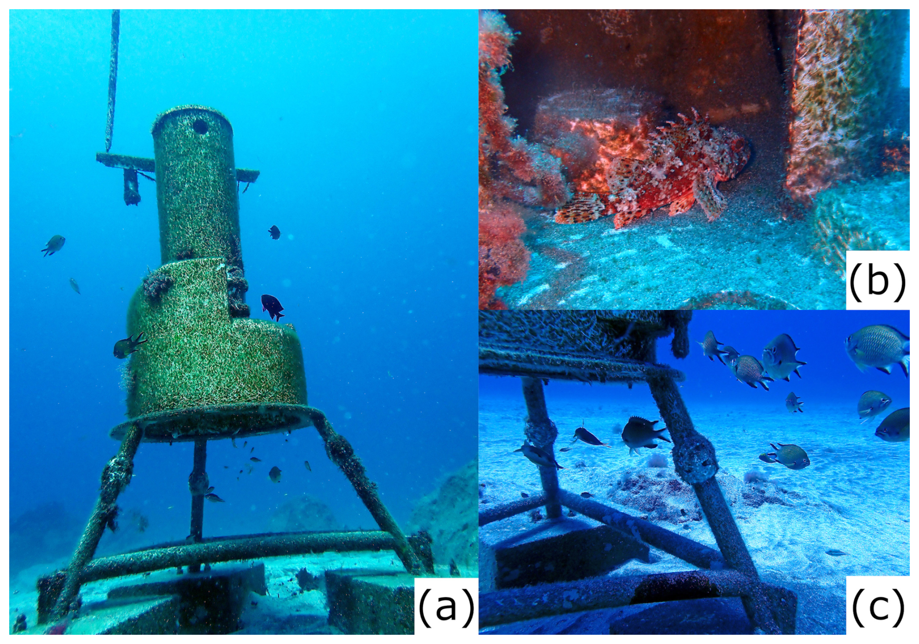
Figure 11 (A) a group of Chromis limbata, swimming near and under the monitoring station (photo taken in 5 April 2024), (b) Scorpaena maderensis using the station as a shelter (photo taken in 24 April 2024), and (c) detail of a Chromis limbata group swimming close and under the monitoring station (photo taken in 25 April 2024). Photos by: Isabelle Peeters.

The results of the present study showed that the installation of artificial reefs may trigger carbon immobilization and benthic biomass generation in a few months. These processes eventually benefit pelagic and benthic communities that help maintain the local biodiversity and also provide aesthetic value to an otherwise unattractive coastal shallow environment. This attribute sustains that the installation of artificial reefs may surely contribute to the development of more ecosystem services (e.g., cultural) in the area.

5 Conclusions

After 18 months of observations (544 d) of environmental conditions for the shallow coastal environment to the south of Tenerife, it was observed that there were no physical (temperature, turbidity, light and water currents), chemical (dissolved oxygen) and biological (chlorophyll a) limitations for benthic biomass development. The biomass and organic carbon (e.g., blue carbon) generated in this oligotrophic area were lower than the amounts observed for the main blue carbon ecosystems at a global scale including those at high-latitude settings; however, they were similar to Mediterranean gorgonian (e.g., soft coral) ecosystems. Together with blue carbon development, the submarine station became a structure able to provide different ecosystem services such as primary production (provisioning ecosystem service), carbon sequestration, fish nursery and shelter, biodiversity pool maintenance (regulating and maintenance ecosystem service) and knowledge (cultural ecosystem service). The blue carbon generated was rapidly (at least 7 months) transferred and incorporated into the local food web. The present study also demonstrates the potential of the oligotrophic coastal ecosystem to the south of Tenerife to generate benthic fauna on artificial substrates in a few months. Further, the observed results make clear that this shallow coastal ecosystem is a good candidate for benthic ecosystem restoration efforts, which eventually, may have the attribute to provide further ecosystem services such as cultural benefits (e.g., recreational).