A T-DINEOF model for multiple oceanic variables reconstruction

Satellite-derived oceanic data are frequently affected by cloud cover, resulting in spatiotemporal gaps. The Multi-DINEOF method is widely used to reconstruct multiple oceanic variables. However, Multi-DINEOF essentially remains a matrix-based DINEOF approach and does not fully leverage the correlations among multiple variables. To address this limitation, this study proposes the T-DINEOF model, aiming to improve the accuracy of reconstructing multiple oceanic variables simultaneously. When applied to sea surface temperature (SST), sea surface chlorophyll a (SCHL), and sea surface wind (SSW) collectively, T-DINEOF reduces root mean square error (RMSE) by 12.9 %, mean absolute error (MAE) by 13.8 %, and mean absolute percentage error (MAPE) by 11.9 % compared to Multi-DINEOF. For each individual oceanic variable, T-DINEOF outperforms both Multi-DINEOF and the original DINEOF methods, reducing RMSE by 9.0 % and 14.7 %, MAE by 10.5 % and 14.6 %, and MAPE by 13.7 % and 13.4 % for SST; reducing RMSE by 9.3 % and 11.8 %, MAE by 9.9 % and 13.4 %, and MAPE by 8.3 % and 11.8 % for SCHL; and reducing RMSE by 16.6 % and 3.7 %, MAE by 16.8 % and 3.5 %, and MAPE by 16.4 % and 3.1 % for SSW. Additionally, T-DINEOF proves effective in regions with a high proportion of missing data and in cases of low data correlation.

1 Introduction

Satellite-derived oceanic observations are the primary source of data for analyzing large-scale, time-series oceanic features. However, due to the limited penetration of visible and infrared bands, these data are often affected by cloud cover, resulting in spatiotemporal gaps. This discontinuity limits their practical application. To mitigate the impact of missing values, long-term averaged data are widely used in many oceanic analyses (Sun et al., 2019a; Bonelli et al., 2022; Zemskova et al., 2022). However, these data often smooth out ocean characteristics and cannot detect short-term or sudden ocean phenomena. Therefore, reconstruction of missing satellite-derived data is receiving increasing attention.

Spatial interpolation methods have already been used to address the issue of missing data. Kriging interpolation, a geostatistical method, was employed to generate complete satellite-derived sea surface temperature (SST) and salinity data for Chesapeake Bay (Urquhart et al., 2013). Additionally, optimal interpolation (OI) is a common method for satellite-derived oceanic data reconstruction (Reynolds and Smith, 1994, 2007; Fieguth et al., 1998). Several OI-based SST datasets, such as NOAA OISST (https://www.ncei.noaa.gov/products/optimum-interpolation-sst, last access: 17 June 2026), and Extended Reconstructed SST (ERSST, https://www.ncei.noaa.gov/products/extended-reconstructed-sst, last access: 17 June 2026), have been used to understand and predict climate system variations (Pawar and San, 2022). The OI method assesses unknown values by combining multiple existing observations with a prior estimate, thereby minimizing the error variance of the predictive outputs. However, this method may artificially smooth the reconstructed fields, limiting the detection of mesoscale features (Martin et al., 2023).

Beckers and Rixen (2003) proposed the Data Interpolating Empirical Orthogonal Function (DINEOF) method, which can be considered a self-consistent data reconstruction method. In the DINEOF method, original time-series satellite-derived oceanic data are transformed into a spatiotemporal matrix. An iterative approach is then applied to this matrix to obtain the optimal EOF mode, and missing values are subsequently reconstructed based on this optimal EOF mode. Compared to the OI method, DINEOF achieves similar reconstruction accuracy with less computational cost and without requiring prior knowledge (Beckers et al., 2006). Therefore, this method has been widely applied to the reconstruction of satellite-derived oceanic variable fields (Alvera-Azcárate et al., 2016; Ji et al., 2018; Liu and Wang, 2018, 2023; Binh et al., 2022). In recent years, several improved DINEOF methods have also been proposed. To enhance the temporal continuity of time-series satellite-derived oceanic data, Alvera-Azcárate et al. (2009) applied a temporal filter technique before the EOF decomposition step in DINEOF. Moreover, because DINEOF aims to optimally reconstruct the overall spatiotemporal matrix while ignoring local optimal reconstruction, Ping et al. (2015) proposed the I-DINEOF method. This method divides the spatiotemporal data into multiple subregions and performs optimal reconstruction for each subregion, thereby improving reconstruction accuracy. Furthermore, the iterative procedure in DINEOF involves significant computational effort, and the optimal EOF mode may not be the best option for intermediate spatiotemporal matrices. Ping et al. (2016) proposed the VE-DINEOF method, which performs optimal reconstruction for each intermediate iterative matrix. In VE-DINEOF, the optimal EOF mode changes progressively with each iteration, thereby improving the reconstruction accuracy and speed of the DINEOF method.

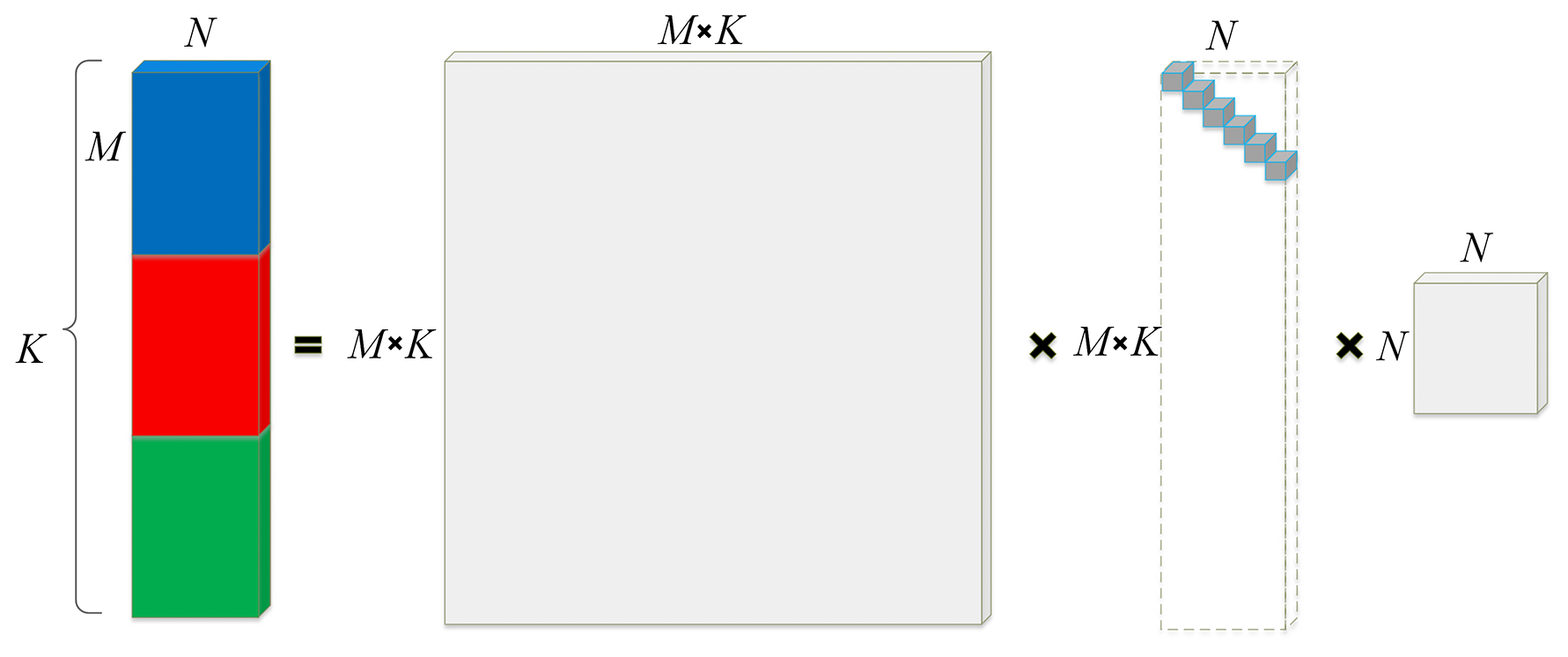
In addition to reconstructing a single oceanic variable, Alvera-Azcárate et al. (2007) proposed a multivariate DINEOF method (Multi-DINEOF) for the reconstruction of multiple ocean variables. This method comprehensively considers the inherent spatiotemporal correlations between these variables, thereby improving reconstruction accuracy. Similarly, Wang et al. (2019) adopted the Multi-DINEOF approach to generate a complete long-term sea surface chlorophyll a (SCHL) dataset based on the Sea-viewing Wide Field-of-view Sensor (SeaWiFS) and Moderate Resolution Imaging Spectroradiometer (MODIS) SCHL products. Wang et al. (2023) utilized wind field data, photosynthetically active radiation (PAR) data, SST data, sea surface salinity (SSS) data, sea surface density (SSD) data, mixed layer depth (MLD) data, sea surface height (SSH) data, and Hybrid Coordinate Ocean Model (HYCOM) reanalysis data as inputs for the Multi-DINEOF method to reconstruct a daily SCHL dataset in the Bay of Bengal. However, as shown in Fig. 1, the Multi-DINEOF method essentially remains a matrix-based DINEOF approach. It first transforms the input multivariate data into a matrix and then applies the original DINEOF approach to reconstruct the missing values. In Fig. 1, multivariate data are represented by different colors. M represents the spatial size of a specific input oceanic variable, K is the overall spatial size of multivariate data, and N represents the number of input oceanic variable images. The first matrix on the right-hand side represents the spatial modes obtained from the singular value decomposition (SVD), the second matrix is the singular value matrix, and the third matrix is the temporal modes. Therefore, the Multi-DINEOF method cannot fully exploit the intrinsic correlations among multiple variables, as different parameters (e.g., SST, SCHL, and SSW) are forced to be represented along the same dimension. Consequently, the extracted principal components may contain mixed and heterogeneous signals, hindering the identification of genuine inter-variable relationships and reducing the physical interpretability of the results. In addition, Multi-DINEOF is limited to characterizing pairwise (second-order) correlations and thus cannot effectively capture higher-order interactions across spatial, temporal, and variable dimensions. This limitation highlights the need to develop an advanced multivariate DINEOF framework that can comprehensively utilize these inter-variable dependencies.

Figure 1 Matrix decomposition in the Multi-DINEOF method.

Multivariate data essentially take the form of a third-order tensor. Therefore, compared with matrix-based reconstruction, applying a third-order tensor formulation can better preserve the intrinsic correlations among various variables and consequently improve reconstruction accuracy. Tensor decomposition represents data as a higher-order array (e.g., space × time × variable), thereby maintaining the native multi-dimensional structure of the dataset. This framework enables the simultaneous extraction of spatial, temporal, and inter-variable modes, preserving the inherent coupling among dimensions. Furthermore, each decomposed mode corresponds to a distinct physical meaning (e.g., spatial pattern, temporal variation, or variable contribution), which enhances both the interpretability and physical consistency of the analysis. Current research on the tensor decomposition has made significant progress, with several decompositions developed, such as higher order SVD (Kolda and Bader, 2009) and hierarchical SVD (Grasedyck, 2010). Kilmer et al. (2008) proposed the tensor SVD (T-SVD) decomposition technique, treating a third-order tensor as a matrix with each element being a tube. The tube-based strategy gives the T-SVD decomposition a form similar to the matrix SVD decomposition (Zeng and Ng, 2020). Therefore, the T-SVD decomposition can be easily integrated into the original DINEOF method. The T-SVD technique has been widely used in facial recognition (Hao et al., 2013), image denoising and reconstruction (Zhang et al., 2014; Zhang and Aeron, 2017; Hu et al., 2017a, b; Zhou et al., 2018; Sun et al., 2019b). Consequently, this study proposed a third-order tensor DINEOF model named T-DINEOF, based on the T-SVD decomposition. The effectiveness of the proposed T-DINEOF model for both overall and individual oceanic variables is demonstrated by comparing it with the Multi-DINEOF method and the original DINEOF method.

The structure of the remainder of this manuscript is as follows: materials will be introduced in the next section; the proposed T-DINEOF model will be presented in Sect. 3; comparisons of the reconstruction accuracies for both overall and individual oceanic variables will be demonstrated and analyzed in Sect. 4; the details of the proposed T-DINEOF model will be discussed in Sect. 5; and finally, conclusions will be given in Sect. 6.

2 Materials

This study used monthly L3 mapped 4 km MODIS Aqua satellite-derived SST and SCHL data from April 2015 to December 2022, which are available for download from Ocean Color (https://oceancolor.gsfc.nasa.gov/, last access: 17 June 2026) as well as monthly approximately 25 km L3 AMSR2 10 m above sea surface wind (SSW) version 8.2 data, which can be downloaded from Remote Sensing Systems (RSS, https://remss.com/missions/amsr/, last access: 17 June 2026), as experimental data. Due to the unavailability of SSW data for August and September 2022, the SST and SCHL data for the same period were also removed. Consequently, the number of input images for each oceanic variable is 91, indicating that the temporal dimension is 91. As shown in Eq. (1), long-wave infrared bands 11 and 12 µm aboard MODIS are employed to retrieve SST products based on a modified version of the nonlinear SST algorithm (Walton et al., 1998; Jia and Minnett, 2020). The combined OC3 $/$ OC4 (OCx) band ratio algorithm (O'Reilly and Werdell, 2019, Eq. 2) and the color index (CI, Hu et al., 2019, Eq. 3), which establish the relationship between SCHL and spectral remote sensing reflectances (R_rs), are used to retrieve SCHL products. Channels that match the low frequency, specifically the 10.65 GHz footprint, are used to retrieve SSW products because they are less affected by the atmosphere and rain. Due to the similar ascending time (13:30 local time), oceanic variables derived from these two satellites are obtained under similar sea conditions.

$$\begin{array}{}\text{(1)}& \begin{array}{rl}& \text{SST}=ai{j}_{\mathrm{0}}+ai{j}_{\mathrm{1}}{\text{BT}}_{\mathrm{11}\mathrm{\mu }\mathrm{m}}+ai{j}_{\mathrm{2}}({\text{BT}}_{\mathrm{11}\mathrm{\mu }\mathrm{m}}-{\text{BT}}_{\mathrm{12}\mathrm{\mu }\mathrm{m}})T_{\text{sfc}}\\ & +ai{j}_{\mathrm{3}}\left(\sec \right(\mathit{\theta })-\mathrm{1})({\text{BT}}_{\mathrm{11}\mathrm{\mu }\mathrm{m}}-{\text{BT}}_{\mathrm{12}\mathrm{\mu }\mathrm{m}})+ai{j}_{\mathrm{4}}\text{(mirror)}\\ & +ai{j}_{\mathrm{5}}\left({\mathit{\theta }}^{*}\right)+ai{j}_{\mathrm{6}}\left({\mathit{\theta }}^{\mathrm{2}}\right)\end{array}\end{array}$$

where BT_11 µm and BT_12 µm are the brightness temperatures at 11 and 12 µm, respectively; θ is the satellite zenith angle; T_sfc is the reference temperature; and aij₀ to aij₆ are regression coefficients determined regionally. The terms “mirror” and “θ^*” represent correction factors associated with viewing geometry and instrument calibration.

$$\begin{array}{}\text{(2)}& {\displaystyle }{\log }_{\mathrm{10}}\left(\text{SCHL}\right)=b_{\mathrm{0}}+\sum _{i=\mathrm{1}}^{\mathrm{4}}{b}_i{\left({\log }_{\mathrm{10}}\left({\displaystyle \frac{R_{\text{rs}}\left({\mathit{\lambda }}_{\text{blue}}\right)}{R_{\text{rs}}\left({\mathit{\lambda }}_{\text{green}}\right)}}\right)\right)}^i\text{(3)}& {\displaystyle }\begin{array}{rl}{\log }_{\mathrm{10}}& \left(\text{SCHL}\right)=-\mathrm{0.4287}+\mathrm{230.47}\times \mathit{\left\{}{R}_{\text{rs}}\right({\mathit{\lambda }}_{\text{green}})\\ & -\left[R_{\text{rs}}\right({\mathit{\lambda }}_{\text{blue}})+({\mathit{\lambda }}_{\text{green}}-{\mathit{\lambda }}_{\text{blue}})/({\mathit{\lambda }}_{\text{red}}-{\mathit{\lambda }}_{\text{blue}})\\ & \cdot \left(R_{\text{rs}}\right({\mathit{\lambda }}_{\text{red}})-R_{\text{rs}}({\mathit{\lambda }}_{\text{blue}}\left)\right)\left]\mathit{\right\}}\end{array}\end{array}$$

where R_rs represents the spectral reflectance, λ is the central wavelength of the target spectral band, and the coefficients b₀−b₄ are sensor-specific parameters.

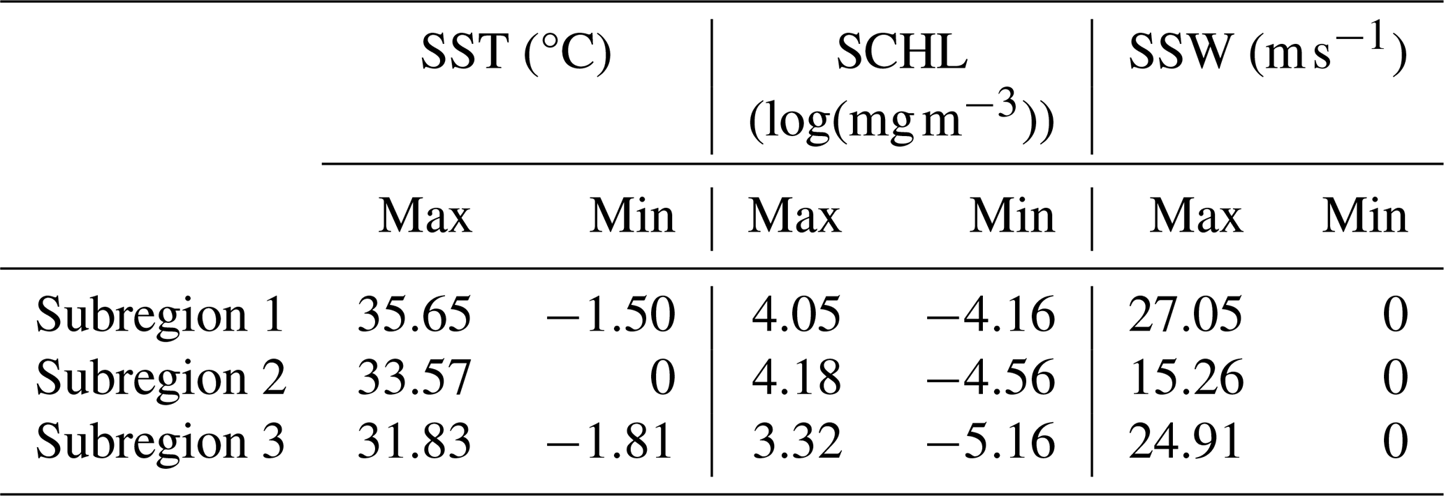
Before constructing the third-order tensor, it is necessary to process the input data. Each MODIS SST pixel has a corresponding numeric quality level, with level 0 being the highest quality and level 4 being the lowest. In this study, only pixels with quality levels 0 (best) and 1 (good/acceptable) were flagged as existing pixels. During the reconstruction stage, due to the log-normal distribution of SCHL data (Campbell, 1995), the log-transformed SCHL data were used in the third-order tensor. Therefore, during the accuracy analysis stage, an inverse log-transformation was applied to the reconstructed SCHL data. According to the RSS website, SSW values greater than 50 or less than 0 were considered missing values in this study. To address the difference in spatial resolution between the MODIS SST and SCHL data and the AMSR2 SSW data, the SST and SCHL data were downscaled to the same resolution as the SSW data using the nearest-neighbor interpolation method. In addition, land areas in the spatially registered SST, SCHL, and SSW datasets were masked out using the land mask provided with the SSW data, which was generated by resampling the high-resolution MODIS land mask onto the target footprint. Due to the large uncertainties in satellite-derived oceanic parameters at high latitudes (Hoyer et al., 2012; Jia et al., 2024), and in order to reduce computational burden, this study focuses on mid-to-low latitude regions; therefore, the area between 60° N and 60° S was chosen as the experimental region. As shown in Fig. 2a, due to limitations in computational power, the experimental area was divided into three subregions, each spanning 40° of latitude from north to south (subregions 1–3). Furthermore, a 3×3 median filter was applied to each satellite-derived variable in each subregion to eliminate abnormal values. Since the ranges of SST, SCHL, and SSW are different, the max-min normalization method was used to scale each ocean variable in each subregion to the range [0–1]. The maximum and minimum values of each ocean variable in each subregion are shown in Table 1. In general, compared to SST and SSW data, log-transformed SCHL data are more concentrated, with smaller variations among different subregions. The highest SST in the mid-latitudes of the Northern Hemisphere is slightly higher than that in the equatorial region and the mid-latitudes of the Southern Hemisphere, while the lowest SST varies slightly among different subregions. The maximum SSW values in the mid-latitude regions are significantly higher than those in the equatorial regions.

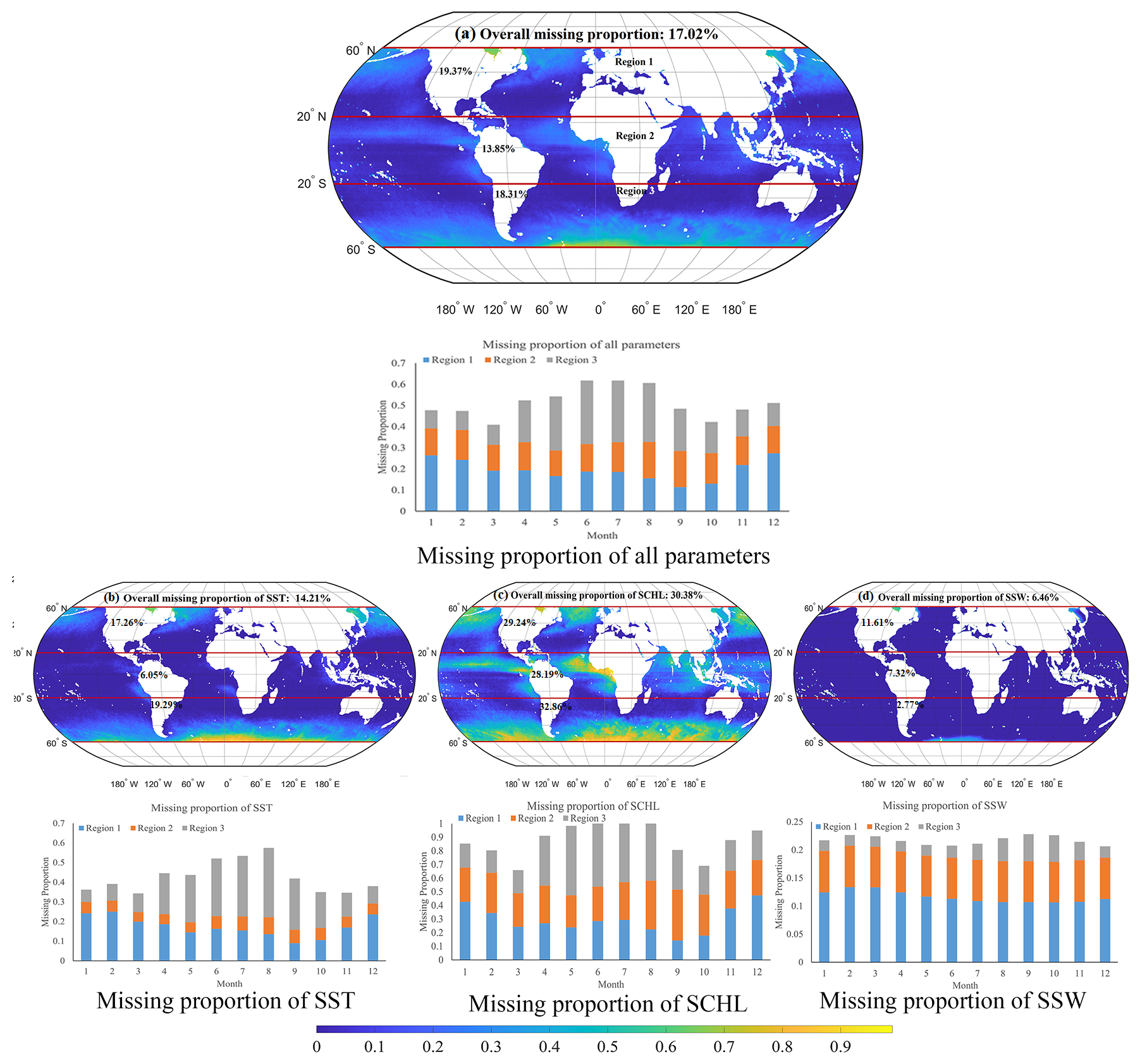
Figure 2 Experimental areas and their corresponding spatiotemporal missing data proportions.

Table 1 Maximum and minimum values of SST, SCHL and SSW in the three subregions.

Each type of processed data was stored in the corresponding m×n matrix, where m is the spatial dimension and n is the temporal dimension. The three matrices generated from the three satellite-derived variables were then combined to form the final third-order tensor. In this study, the dimensions of the final tensor for the three subregions are $\mathrm{119}\mathrm{939}\times \mathrm{91}\times \mathrm{3}$, $\mathrm{174}\mathrm{091}\times \mathrm{91}\times \mathrm{3}$, and $\mathrm{207}\mathrm{779}\times \mathrm{91}\times \mathrm{3}$ after masking out land pixels.

In addition, the spatial and temporal proportions of missing data are shown in Fig. 2. In this study, the missing data ratio was calculated as the total number of missing values in the target variable, or across all three variables – after excluding land-masked areas in the target subregion – divided by the total number of data points in the corresponding tensor dimension or in the entire three-dimensional tensor. Additionally, by categorizing the time series data by date into their respective months, the missing data ratio for each month was obtained using the same method described above. Considering SST, SCHL and SSW data collectively (Fig. 2a), the global proportion of missing data is 17.02 %. The proportions of missing data in subregions 1, 2, and 3 are 19.37 %, 13.85 %, and 18.31 %, respectively, indicating that the equatorial region has a lower proportion of missing data compared to the mid-latitude regions. Typically, the proportions of missing data are higher from June to August than in other months, especially in subregion 3. The proportion of missing data in subregion 2 does not vary significantly across the months, while subregion 1 typically has a lower proportion of missing data from September to October.

The global proportion of missing SST data is 14.21 % (Fig. 2b). In subregions 1–3, the proportions are 17.26 %, 6.05 %, and 19.29 %, respectively, indicating that the proportion in the equatorial region is significantly lower than in the mid-latitude regions. Overall, the proportion of missing SST data is higher from June to August. Subregion 2 shows minimal temporal variation in SST missing data proportions. In contrast, subregions 1 and 3 exhibit opposite trends: from April to October, subregion 3 has higher proportions than subregion 1, peaking from June to August. However, in other months, subregion 1 has higher missing data proportions compared to subregion 3.

The global proportion of missing SCHL data is 30.38 % (Fig. 2c), which is the highest among the three oceanic variables. In subregions 1–3, the proportions are 29.24 %, 28.19 %, and 32.86 %, respectively, showing no significant differences. Overall, the proportions of missing data are typically higher from April to August and in December. In subregion 1, the proportions are lower from August to October but higher from December to January compared to other months. Subregion 2 shows higher missing proportions from August to October, while in the remaining months, the proportions in this subregion do not vary significantly. From April to September, the missing proportions in subregion 3 are obviously higher than in other months.

The global proportion of missing SSW data is 6.46 % (Fig. 2d), indicating that SSW has the most complete data among the three oceanic variables due to the penetration capability of microwave bands. In subregions 1–3, the proportions are 11.61 %, 7.32 %, and 2.77 %, respectively, indicating that the mid-latitudes of the Southern Hemisphere are least affected by missing data. Overall, the proportions of missing data remain relatively stable across months. In February and March, subregion 1 experiences a peak in missing values, while in subregion 3, the peak occurs from August to October. The proportions of missing values in other months for these two subregions do not vary significantly. In subregion 2, the proportion of missing values remains stable throughout the year.

3 Methodology

Currently, several decomposition methods for third-order tensor, such as higher order SVD (Kolda and Bader, 2009) and hierarchical SVD (Grasedyck, 2010), have been proposed. The T-SVD decomposition has a form similar to that of the matrix SVD decomposition (Zeng and Ng, 2020). Therefore, this study incorporated the T-SVD decomposition method into the original DINEOF algorithm and proposed a T-DINEOF model. The algebraic framework of T-SVD is constructed by defining the tensor-tensor product, identity tensor, transpose, orthogonal tensor, and tubal rank (Braman, 2010; Kilmer and Martin, 2011; Kilmer et al., 2013; Kernfeld et al., 2015). Consequently, the decomposition and reconstruction of the third-order tensor based on the T-SVD method are introduced, followed by a detailed explanation of the T-DINEOF model.

3.1 Decomposition and reconstruction of third-order tensor

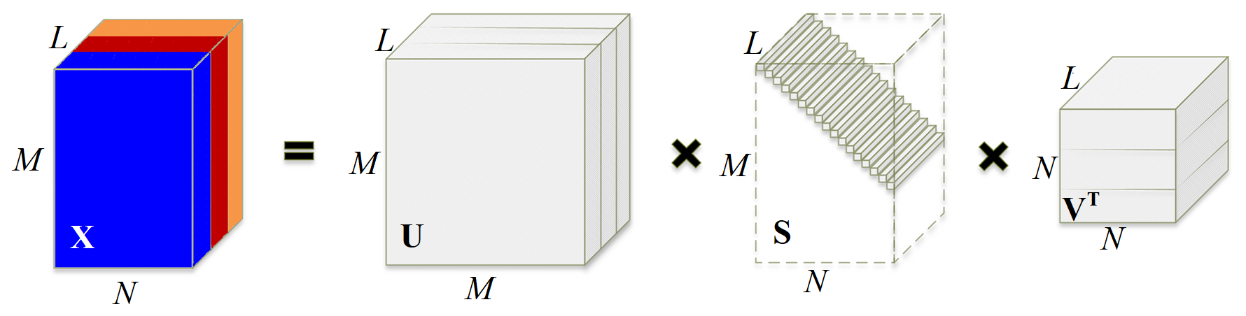
The T-SVD decomposition is the core of the T-DINEOF model and represents an improvement over the original DINEOF algorithm. It can be performed based on Eqs. (4)–(7), with an illustration of the T-SVD decomposition provided in Fig. 3.

$$\begin{array}{}\text{(4)}& X=U\times S\times V^T\end{array}$$

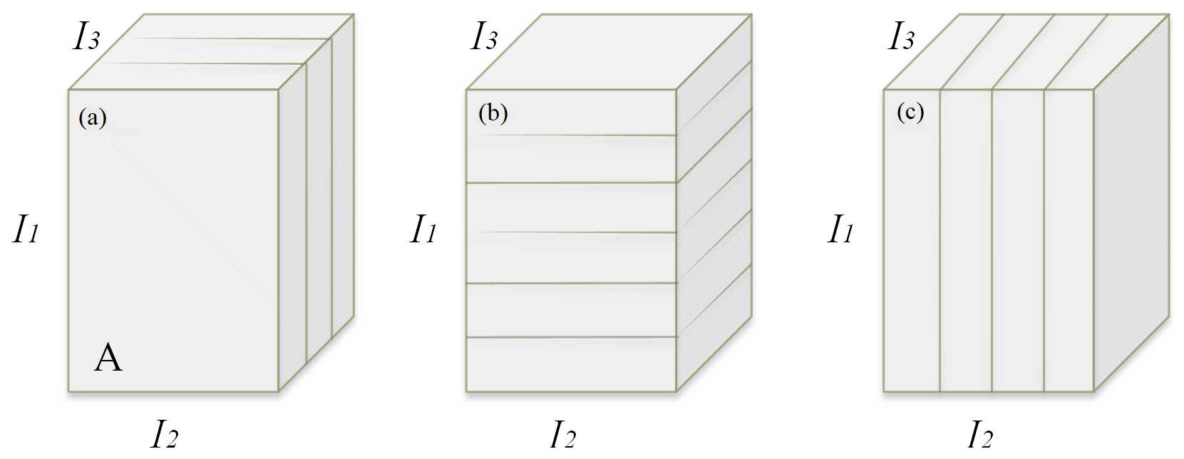
where $\mathbf{X}\in {\mathbf{R}}^{M\times N\times L}$ is the input third-order tensor, and M, N, and L represents the dimensions of the third-order tensor. In this study, since the temporal dimension is 91 and three oceanic variables are used, N and L are 91 and 3, respectively. $\mathbf{U}\in {\mathbf{R}}^{M\times M\times L}$ and $\mathbf{V}\in {\mathbf{R}}^{N\times N\times L}$ are orthogonal tensors, and $\mathbf{S}\in {\mathbf{R}}^{M\times N\times L}$ is an f-diagonal tensor, meaning that each frontal slice of S is a diagonal matrix. T denotes the transpose operation, which involves transposing each frontal slice of a third-order tensor and then reversing the order of the results from the 2nd to the last frontal slice. As shown in Fig. 4a, a frontal slice of a third-order tensor $\mathbf{A}\in {\mathbf{R}}^{I_{\mathrm{1}}\times I_{\mathrm{2}}\times I_{\mathrm{3}}}$ refers to a matrix of size I₁×I₂ taken from a specific value of the third dimension, I₃. The symbol ^* represents the tensor product, which can be defined as follows:

$$\begin{array}{}\text{(5)}& {\displaystyle }{A}^{*}B=\text{fold}\left(\text{bcirc}\right(A)\cdot \text{unfold}(B\left)\right)\text{(6)}& {\displaystyle }\text{bcirc}\left(A\right)=\left[\begin{array}{cccc}{A}^{\left(\mathrm{1}\right)}& A^{\left(I_{\mathrm{3}}\right)}& \mathrm{\dots }& A^{\left(\mathrm{2}\right)}\\ A^{\left(\mathrm{2}\right)}& A^{\left(\mathrm{1}\right)}& \mathrm{\dots }& A^{\left(\mathrm{3}\right)}\\ \mathrm{⋮}& \mathrm{⋮}& \mathrm{\ddots }& \mathrm{⋮}\\ A^{\left(I_{\mathrm{3}}\right)}& A^{(I_{\mathrm{3}}-\mathrm{1})}& \mathrm{\dots }& A^{\left(\mathrm{1}\right)}\end{array}\right]\text{(7)}& {\displaystyle }\text{unfold}\left(A\right)=\left[\begin{array}{c}{A}^{\left(\mathrm{1}\right)}\\ A^{\left(\mathrm{2}\right)}\\ \mathrm{⋮}\\ A^{\left(I_{\mathrm{3}}\right)}\end{array}\right],\text{fold}\left(\text{unfold}\right(A\left)\right)=A\end{array}$$

where $\mathbf{A}\in {\mathbf{R}}^{I_{\mathrm{1}}\times I_{\mathrm{2}}\times I_{\mathrm{3}}}$ and $\mathbf{B}\in {\mathbf{R}}^{I_{\mathrm{2}}\times I_{\mathrm{4}}\times I_{\mathrm{3}}}$ are two third-order tensors, and the output size of A^*B is $I_{\mathrm{1}}\times I_{\mathrm{4}}\times I_{\mathrm{3}}$. A^(m) represents the mth frontal slice. The unfold operation maps the third-order tensor A into a matrix of size I₁I₃×I₂, while fold is its inverse transformation. The symbol ⋅ represents matrix multiplication.

Figure 3 Illustration of T-SVD decomposition.

Figure 4 An example of (a) frontal slices, (b) horizontal slices, and (c) lateral slices.

After decomposing X based on Eq. (4), the reconstructed third-order tensor can be obtained using Eq. (8).

$$\begin{array}{}\text{(8)}& X_{\text{recon}}=\sum _{p=\mathrm{1}}^{q}U(:,p,:{)}^{*}S(p,p,:{)}^{*}V(p,:,:{)}^T\end{array}$$

where X_recon signifies the reconstructed third-order tensor, and q represents the number of modes. In the original DINEOF algorithm, the pth singular vectors extracted from the U and transposed V matrices, along with the pth singular value extracted from the S matrix, are multiplied to form the reconstruction matrix for the pth mode. The reconstruction matrices for the pth mode and all previous modes are then summed to obtain the final reconstruction matrix. In the T-DINEOF model, the pth lateral and horizontal slices extracted from the third-order tensor U and transposed third-order tensor V, along with the pth singular vector extracted from the third-order tensor S, are used to construct the reconstructed tensor for the pth mode. Similarly, the reconstructed third-order tensors for the pth mode and all previous modes are summed to obtain the final reconstruction tensor. It can be seen that the original DINEOF algorithm decomposes a two-dimensional matrix into orthogonal spatial and temporal modes, capturing only pairwise correlations between these dimensions. In contrast, T-DINEOF extends this concept to higher-order tensors, decomposing data simultaneously along multiple dimensions such as space, time, and variable. By operating directly in the tensor domain, T-DINEOF preserves the intrinsic multi-dimensional structure of the data and explicitly models interactions across the variable dimension. This allows T-DINEOF to capture synergistic patterns arising from the coupled variations among multiple variables – patterns that the conventional DINEOF, constrained to a flattened two-dimensional representation, cannot inherently represent.

3.2 T-DINEOF model

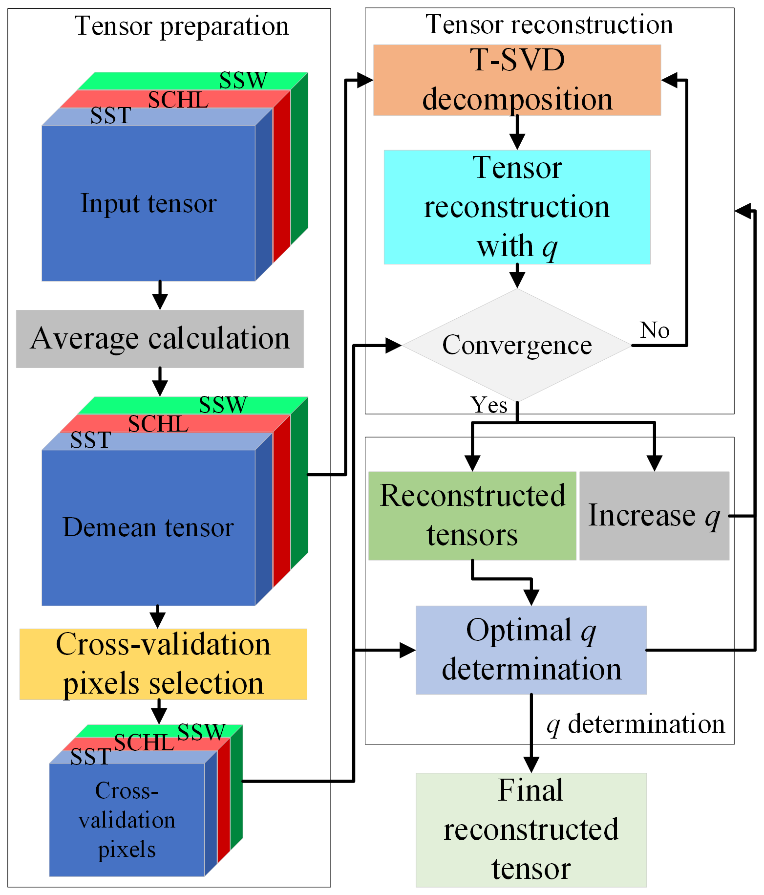
In this study, the T-DINEOF model was implemented using Matlab R2023b. The flowchart of T-DINEOF is shown in Fig. 5, which consists of three main modules: Tensor preparation (Steps 1 and 2), Tensor reconstruction (Step 3), and q determination (Step 4). Once the optimal q is obtained, the final reconstructed tensor can be generated through the Tensor reconstruction module. The specific process of T-DINEOF is as follows:

• (1)

  Spatiotemporal averages calculation. The corresponding spatiotemporal averaged values for SST, SCHL, and SSW data were calculated and then these averages were subtracted from each oceanic variable.

• (2)

  Cross-validation pixels selection. The same cross-validation pixel selection strategy as in the original DINEOF method was adopted, i.e., 3 % of the existing data from the corresponding spatiotemporal matrix of each oceanic variable were randomly selected as cross-validation pixels. In addition, we analyzed the impact of different cross-validation pixel proportions (see Discussion). The results indicate that the choice of proportion has only a minor effect on the reconstruction accuracy, and the 3 % setting performs slightly better overall. During the optimal mode determination phase, these cross-validation pixels were treated as missing pixels. Both the missing pixels and the cross-validation pixels were set to zero (unbiased guess).

• (3)

  Decomposition and reconstruction. The third-order tensor was decomposed first based on Eq. (4), and then reconstructed using Eq. (8) with q=1. After replacing the missing values with the corresponding reconstructed values, the new reconstructed tensor was re-decomposed and the missing values were recalculated. This process was iterated until the root mean square error (RMSE) between previous and current iterations was less than 0.00001 at the cross-validation pixels. To prevent an endless iterative loop and to save computational time, a maximum of 100 iterations was predefined. The RMSE is defined as:

  $$\begin{array}{}\text{(9)}& \text{RMSE}=\sqrt{{\displaystyle \frac{\sum (R-O{)}^{\mathrm{2}}}{l}}}\end{array}$$

  where R is the estimated value, O is the original value, and l is the number of cross-validation pixels.

• (4)

  Optimal q determination. When convergence was achieved or the maximum number of iterations was reached, incremented q by 1 and repeated step (3). In this study, the maximum value of q was set to 100, resulting in the reconstruction of 100 third-order tensors. The RMSEs between the original and the reconstructed values at the cross-validation pixels for various q values were calculated. The optimal q was determined by identifying the value that minimizes the RMSE.

• (5)

  Final reconstruction. Once the optimal q value was determined, repeated step (3), treating the cross-validation pixels in the third-order tensor as existing pixels. The final missing data values were replaced with the corresponding reconstructed values obtained based on the optimal q value.

Figure 5 Flowchart of T-DINEOF.

3.3 Quantitative assessment

The original values and the reconstructed values at the existing pixels were used to assess the performance of the T-DINEOF model along with two other control models. In addition to RMSE, three other evaluation metrics were selected to quantitatively assess the performance: mean absolute error (MAE), coefficient of determination (R²), and mean absolute percentage error (MAPE). These metrics are calculated as follows:

$$\begin{array}{}\text{(10)}& {\displaystyle }\text{MAE}={\displaystyle \frac{\sum \mathrm{|}{R}_{\text{exist}}-O_{\text{exist}}\mathrm{|}}{l_{\text{exist}}}}\text{(11)}& {\displaystyle }{R}^{\mathrm{2}}=\mathrm{1}-{\displaystyle \frac{\sum (O_{\text{exist}}-R_{\text{exist}}{)}^{\mathrm{2}}}{\sum (O_{\text{exist}}-\stackrel{\mathrm{‾}}{O_{\text{exist}}}{)}^{\mathrm{2}}}}\text{(12)}& {\displaystyle }\text{MAPE}={\displaystyle \frac{\sum \mathrm{|}(R_{\text{exist}}-O_{\text{exist}})/O_{\text{exist}}\mathrm{|}}{l_{\text{exist}}}}\times \mathrm{100}\mathit{\%}\end{array}$$

where R_exist and O_exist signify the reconstructed and original values at the existing pixels within all images in the study area during the target period, respectively, and l_exist indicates the number of existing pixels. Lower RMSE, MAE, and MAPE values, along with higher R² values, signify better reconstruction performance.

4 Results

4.1 Performance of T-DINEOF

In this section, the three study areas for all three variables SST, SCHL and SSW are analyzed collectively to evaluate the performance of the T-DINEOF model. Since there are no true values at the missing points for comparison, the reconstructed values at the existing points are compared with the corresponding true values to assess the model's performance. Due to differences in magnitude, the MAPE value is divided by 10 in the radar chart. As shown in Fig. 6, compared with the Multi-DINEOF method, T-DINEOF performs better in terms of RMSE, MAE, and MAPE values, while achieving a comparable R² value (0.9989 vs. 0.9986). This indicates that the T-DINEOF model for third-order tensor reconstruction is more effective in utilizing the correlations between various variables than the Multi-DINEOF method for matrix reconstruction, thereby improving reconstruction accuracy. Specifically, compared to the Multi-DINEOF method, the T-DINEOF model reduces RMSE by 12.9 %, MAE by 13.8 %, and MAPE by 11.9 %.

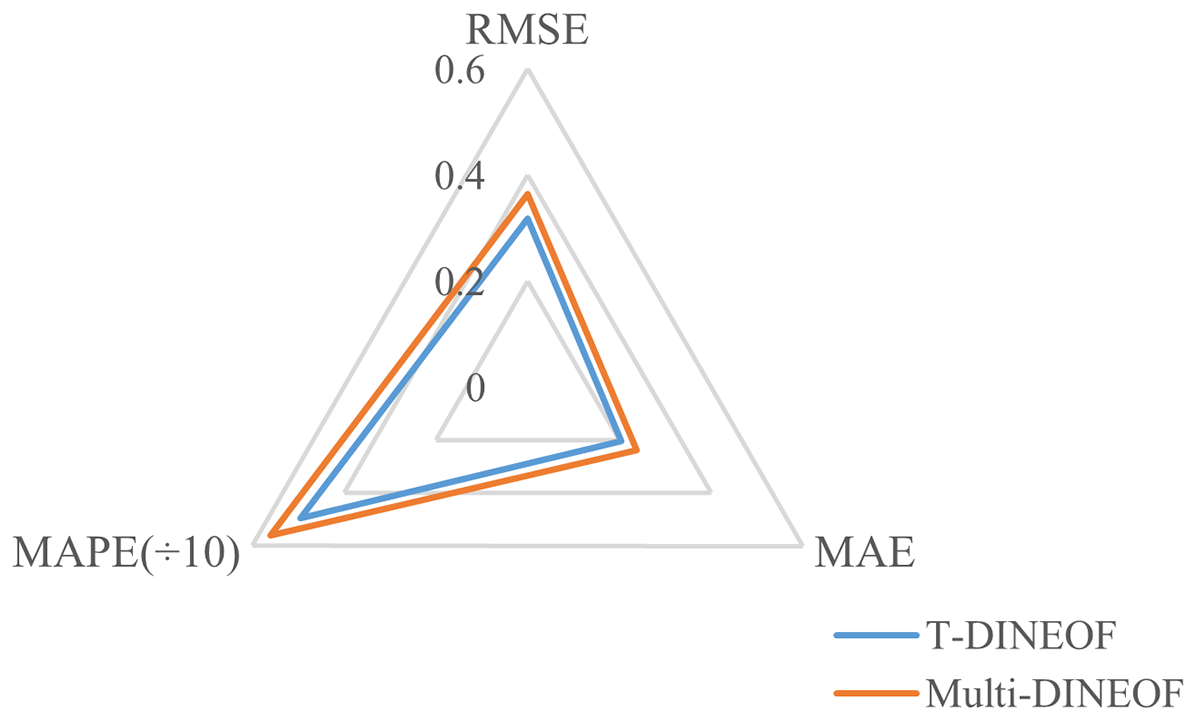
Figure 6 Radar chart of global statistical accuracies for all three variables SST, SCHL and SSW. The blue and red polygons represent T-DINEOF and Multi-DINEOF, respectively.

The scatter density plots comparing the reconstruction values from T-DINEOF and Multi-DINEOF with the original values are shown in Fig. 7. Generally, the reconstruction values from both T-DINEOF and Multi-DINEOF are closely aligned with the 1:1 line, indicating that both methods produce reasonable reconstruction results. However, both methods tend to underestimate high-value pixels, as highlighted by the red ellipse. By analyzing the scatterplot distributions of SST, SCHL, and SSW, it was found that these underestimated values mainly originate from the SCHL data in subregion 1 and subregion 2, indicating that SCHL values may be underestimated in these two subregions. Although the scatter plots of the two methods appear similar, the T-DINEOF model demonstrates superior statistical accuracy compared to the Multi-DINEOF method.

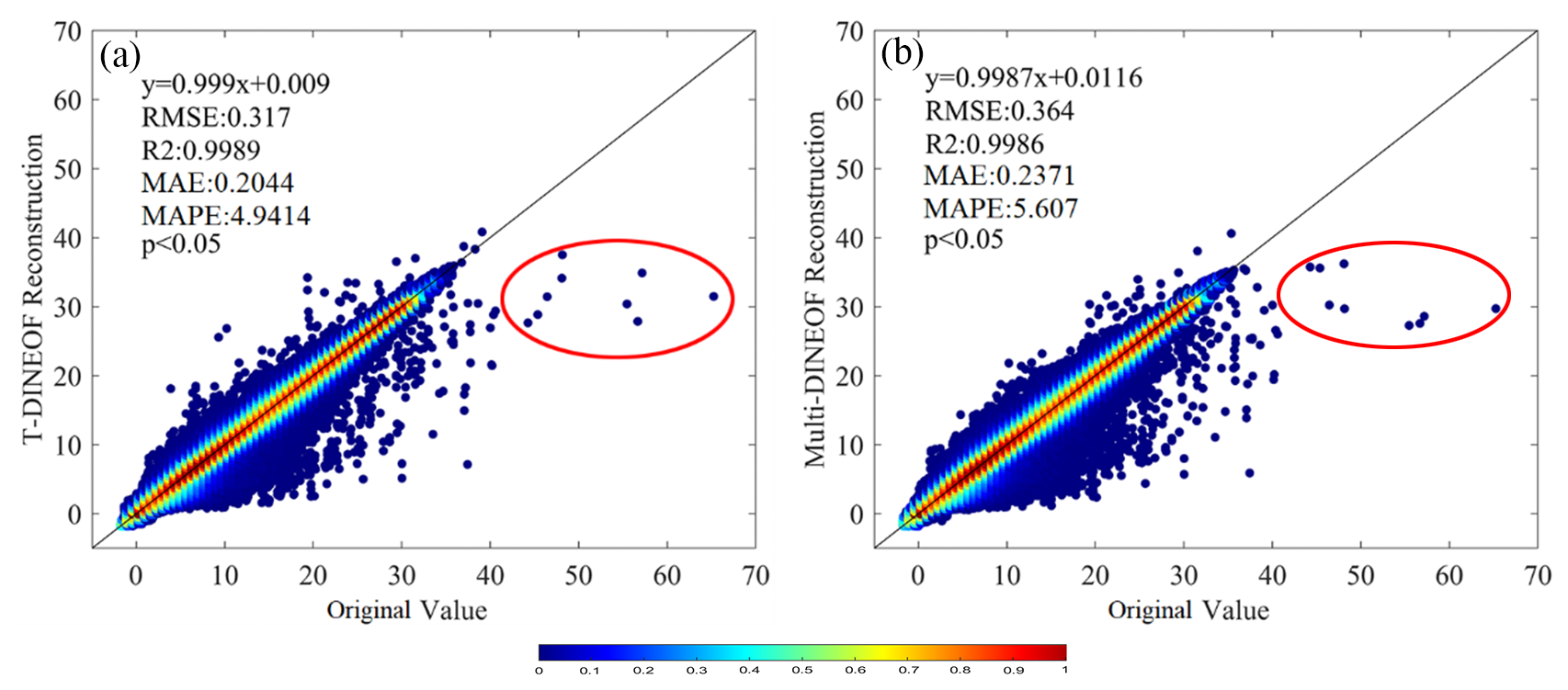
Figure 7 Scatter density plots for SST, SCHL, and SSW, obtained from (a) T-DINEOF and (b) Multi-DINEOF. Values are shown in their original physical units after inverse max-min normalization, using the parameters provided in Table 1: SST in °C, SCHL in mg m⁻³, and SSW in m s⁻¹.

Next, the reconstruction accuracies for each ocean variable are analyzed separately. In this section, the univariate DINEOF method (Single-DINEOF) is also included for comparative analysis alongside the Multi-DINEOF method. For SST data (Fig. 8a), the T-DINEOF model achieves the lowest RMSE, MAE, and MAPE values compared to both the Multi-DINEOF and Single-DINEOF methods, indicating superior reconstruction accuracy for SST. Specifically, T-DINEOF reduces RMSE by 9.0 % and 14.7 %, MAE by 10.5 % and 14.6 %, and MAPE by 13.7 % and 13.4 %, respectively, compared to the Multi-DINEOF and Single-DINEOF methods.

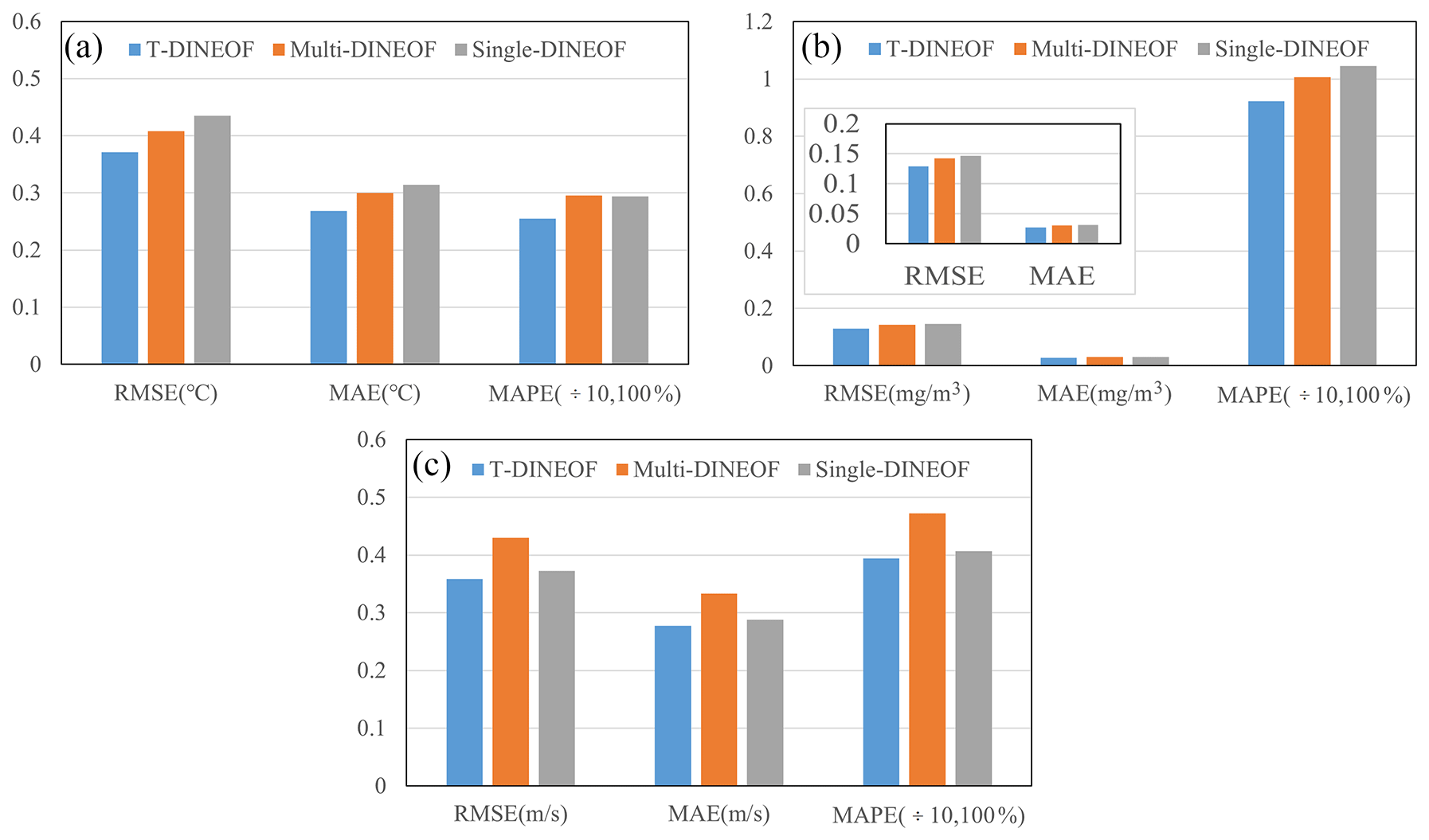
Figure 8 Comparison of accuracies for global (a) SST, (b) SCHL and (c) SSW obtained from T-DINEOF, Multi-DINEOF, and Single-DINEOF.

The reconstruction accuracies for SCHL are shown in Fig. 8b, with a magnified view of RMSE and MAE in the subplot. The T-DINEOF model again demonstrates the highest reconstruction accuracy, achieving the lowest RMSE, MAE, and MAPE values for SCHL. Compared to the Multi-DINEOF and Single-DINEOF methods, T-DINEOF reduces RMSE by 9.3 % and 11.8 %, MAE by 9.9 % and 13.4 %, and MAPE by 8.3 % and 11.8 %, respectively. Additionally, both multivariate reconstruction methods (T-DINEOF and Multi-DINEOF) outperform the Single-DINEOF method for SST and SCHL, suggesting that, as seen in previous research (Alvera-Azcárate et al., 2007; Wang et al., 2023), multivariate methods better utilize the correlations between different oceanic variables and the target variable, leading to improved reconstruction accuracy. In addition, the Multi-DINEOF method reconstructs missing values by reshaping multiple spatiotemporal variables into a two-dimensional matrix for decomposition. As a result, the spatial information of multiple oceanic variables is combined into a single matrix. During reconstruction, the resulting optimal spatiotemporal mode represents a compromise among the variables, which may lead to reduced reconstruction accuracy for individual parameters. In contrast, the T-DINEOF method integrates multiple oceanic variables into a three-dimensional tensor. The reconstruction is thus based on an optimal spatiotemporal tensor (as described in Eq. 8), allowing the method to consider the reconstruction accuracy of each variable individually. This approach avoids the compromise inherent in Multi-DINEOF and improves the reconstruction accuracy for each individual oceanic parameter.

As shown in Fig. 8c, T-DINEOF also achieves the best performance for SSW data. Compared to the Multi-DINEOF and Single-DINEOF methods, T-DINEOF reduces RMSE by 16.6 % and 3.7 %, MAE by 16.8 % and 3.5 %, and MAPE by 16.4 % and 3.1 %, respectively. The improvements in reconstruction accuracy for SSW data with T-DINEOF are more significant relative to the Multi-DINEOF method, while the improvements relative to the Single-DINEOF method are comparatively smaller. In the input third-order tensor, the correlation coefficient between SST and SCHL is −0.60, between SCHL and SSW is 0.03, and between SST and SSW is −0.04. This indicates that the correlation between SSW and the other two oceanic variables is weaker than the correlation between SST and SCHL. The low correlation makes it challenging for the Multi-DINEOF method to effectively reconstruct SSW data. However, T-DINEOF can still leverage other oceanic variables to improve the reconstruction accuracy of the target variable, even in cases of low correlation.

In addition to statistical comparisons, visual comparisons of the reconstruction maps from T-DINEOF, Multi-DINEOF, and Single-DINEOF in the northern Pacific are also presented. The SST map for April 2022 serves as an example in this section. As shown in Fig. 9, T-DINEOF (Fig. 9a), Multi-DINEOF (Fig. 9b), and Single-DINEOF (Fig. 9c) all successfully address SST missing values and preserve the overall SST structure. However, the SST map reconstructed with Single-DINEOF exhibits some smoothing of details. The difference maps between the reconstructed SST maps from the three methods and the raw SST (Fig. 9d) reveal that T-DINEOF (Fig. 9e) has smaller differences from the original SST values, with deviations more centered around zero compared to the other methods. In addition, the Multi-DINEOF and Single-DINEOF methods result in some abnormally high values (black ellipses in Fig. 9f and g), which are avoided by T-DINEOF, contributing to its superior performance.

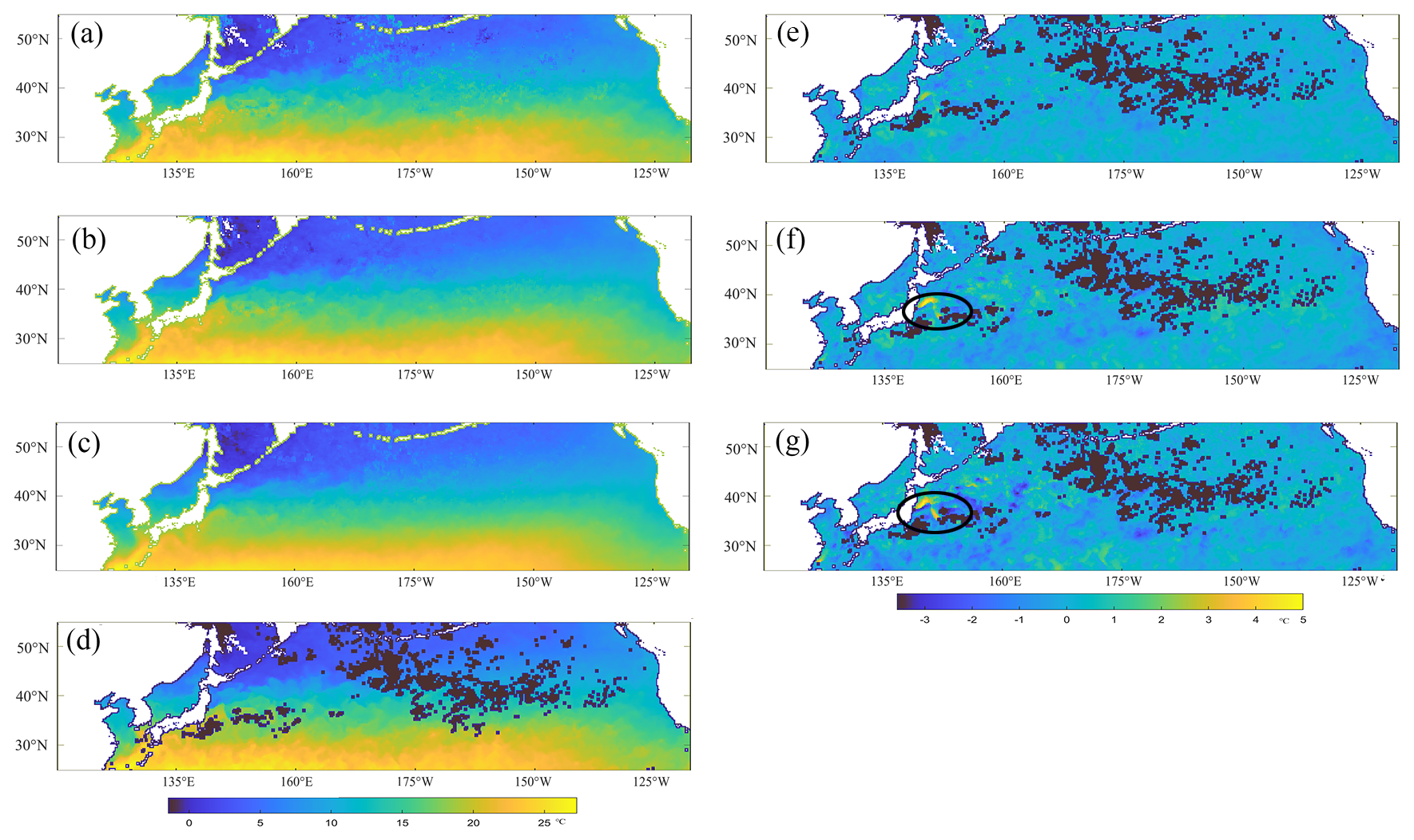
Figure 9 Reconstructed SST maps for April 2022 in the northern Pacific obtained from (a) T-DINEOF, (b) Multi-DINEOF, and (c) Single-DINEOF. (d) is the corresponding raw SST map. Panels (e)–(g) show the difference maps between the reconstructed SST maps from T-DINEOF, Multi-DINEOF, and Single-DINEOF, and the raw SST map.

To analyze the detail-preserving capabilities of Single-DINEOF, Multi-DINEOF, and T-DINEOF, the gradients between adjacent eastward and northward pixels were calculated for the SST, SCHL, and SSW images reconstructed by the three methods. The square root of the sum of squared gradients in the two directions was then used as the pixel gradient magnitude to generate the corresponding gradient maps. The SST gradient maps are shown in Fig. 10, while the gradient maps of SCHL and SSW are presented in Figs. S4 and S5 in the Supplement, respectively. Overall, compared with the Multi-DINEOF (a) and Single-DINEOF (b) methods, the T-DINEOF method (c) produces more gradient information with higher gradient magnitudes, indicating a better preservation of fine-scale details. The Multi-DINEOF and Single-DINEOF methods yield relatively low gradient values in the central and eastern North Pacific, failing to adequately capture the detailed structures in these regions. In contrast, although all three methods produce relatively high gradient values in the western North Pacific, the T-DINEOF method preserves substantially richer details, further demonstrating its advantage in detail-preserving capabilities.

In addition to gradient-map comparisons, we introduced three quantitative metrics to evaluate feature preservation: variance preservation (VP), Structural Similarity Index (SSIM), and anomaly structure (AS). VP was calculated as the ratio of the total variance of the reconstructed field to that of the original field at existing pixels, quantifying the fraction of total variance retained. SSIM was used to assess the structural similarity between reconstructed and original fields by considering luminance, contrast, and spatial structure. AS was computed as the correlation between the reconstructed and original anomaly fields, highlighting the ability to preserve fine-scale variations and key spatial features. For the three study subregions, T-DINEOF yielded VP values of 0.9987, 0.9996, and 0.9981, SSIM values of 0.5626, 0.6011, and 0.5677, and AS values of 0.9992, 0.9998, and 0.9991, respectively.

Although the SSIM values (0.56–0.60) indicate that some local-scale differences remain between reconstructed and original fields, the consistently high VP and AS values demonstrate that the dominant variance and anomaly structures are effectively preserved. Combined with the gradient-map comparisons, these results suggest that T-DINEOF retains the major spatial features and fine-scale structures reasonably well, although some degree of smoothing is still present, which is consistent with the intrinsic characteristics of DINEOF-type low-rank reconstructions.

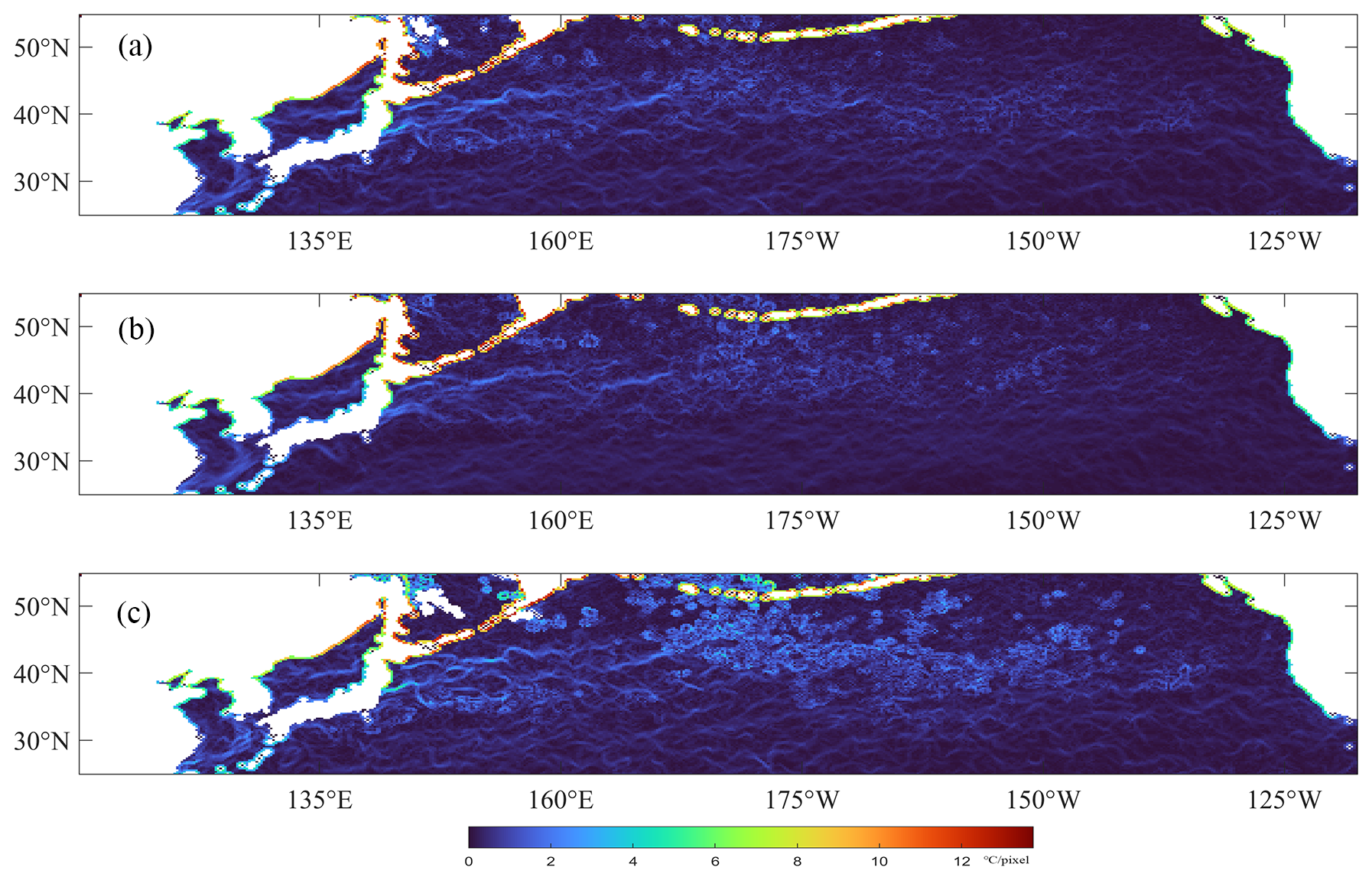
Figure 10 Gradient maps of SST for April 2022 in the northern Pacific obtained from (a) Multi-DINEOF, (b) Single-DINEOF, and (c) T-DINEOF.

The SCHL map for July 2021 illustrates the performance of the reconstruction methods for SCHL. As shown in Fig. 11d, missing data in the northern Pacific are mainly concentrated in the northern area with high SCHL values and parts of the southeastern area. All three methods successfully reconstruct the missing values and maintain the spatial structure of the SCHL data. The reconstructed SCHL data from T-DINEOF (Fig. 11a), Multi-DINEOF (Fig. 11b), and Single-DINEOF (Fig. 11c) are not significantly different, probably due to the narrow range of the log-transformed SCHL data. However, as indicated by the black ellipses in Fig. 11f and g, Multi-DINEOF and Single-DINEOF produce some abnormally high values, which may affect the reconstruction accuracy.

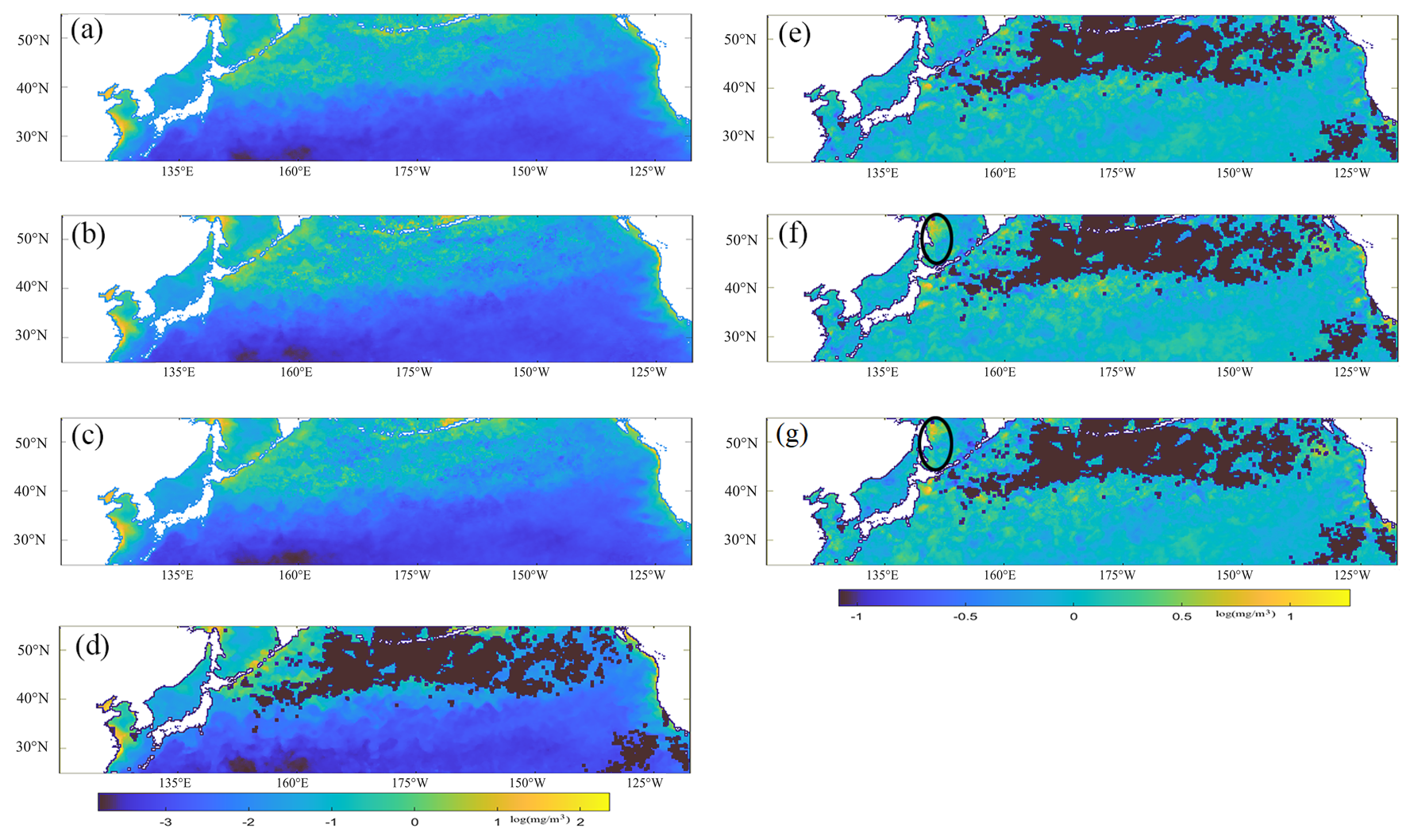
Figure 11 Reconstructed SCHL maps for July 2021 in the northern Pacific obtained from (a) T-DINEOF, (b) Multi-DINEOF, and (c) Single-DINEOF. Panel (d) is the corresponding raw SCHL map. Panels (e)–(g) show the difference maps between the reconstructed SCHL maps from T-DINEOF, Multi-DINEOF, and Single-DINEOF, and the raw SCHL map.

The SSW data for January 2020 is used to evaluate the performance of the reconstruction methods for SSW. Due to limitations in microwave imaging, the SSW data retrieved using the microwave bands of AMSR2 exhibit more gaps in nearshore areas (black ellipse in Fig. 12d), while there are fewer gaps in open ocean areas. While all three methods yield visually similar reconstructions, the difference maps highlight distinct performance differences. The Multi-DINEOF method exhibits significant overestimation and underestimation (black and blue ellipses in Fig. 12f), reflecting lower accuracy. The Single-DINEOF method also shows regions with high and low differences (black and blue ellipses in Fig. 12g) and has a less smooth difference map compared to T-DINEOF (Fig. 12e), which provides a more continuous and accurate reconstruction of SSW.

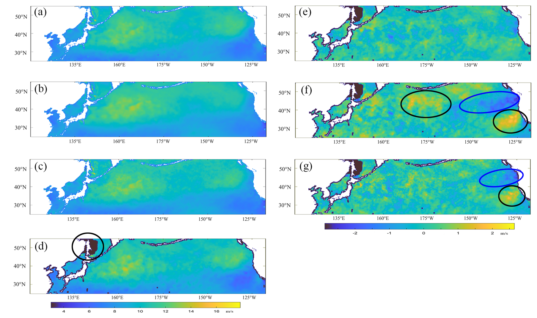
Figure 12 Reconstructed SSW maps for January 2020 in the northern Pacific obtained from (a) T-DINEOF, (b) Multi-DINEOF, and (c) Single-DINEOF. Panel (d) is the corresponding raw SSW map. Panels (e)–(g) show the difference maps between the reconstructed SSW maps from T-DINEOF, Multi-DINEOF, and Single-DINEOF, and the raw SSW map.

Figures 9, 11, and 12 show that T-DINEOF outperforms Single-DINEOF and Multi-DINEOF in specific regions, particularly along the coast. Coastal waters exhibit more complex environmental conditions than the open ocean, resulting in intricate interactions among variables such as SST, SCHL, and SSW. Matrix-based methods, including Single-DINEOF and Multi-DINEOF, cannot fully capture these intrinsic correlations because different parameters are constrained along the same dimension. By contrast, T-DINEOF employs tensor operations to simultaneously extract spatial, temporal, and inter-variable modes, preserving the inherent coupling across dimensions and enabling more accurate reconstruction in complex nearshore environments.

4.2 Accuracy analysis for sub-regions

In this section, the differences in reconstruction methods across various spatiotemporal ranges are analyzed. The reconstruction accuracies of the T-DINEOF and Multi-DINEOF methods for the three subregions are shown in Fig. 13. The radar charts reveal that T-DINEOF consistently outperforms Multi-DINEOF in all three subregions. Specifically, in subregion 2 (the equatorial area), the accuracy magnitudes are lower than those in subregions 1 and 3 (the mid-latitude areas), as indicated by the smaller polygon area on the radar chart. This suggests better reconstruction performance in the equatorial region. Figure 2a shows that the proportion of missing values in the equatorial region is lower than in the mid-latitude regions of both hemispheres. A lower proportion of missing values means more information is available for reconstruction, resulting in higher reconstruction accuracy in the equatorial region. Additionally, the accuracy differences between the two methods are smaller in the equatorial region compared to the mid-latitude areas. This indicates that in regions with a small proportion of missing values, both methods can achieve similar reconstruction accuracy.

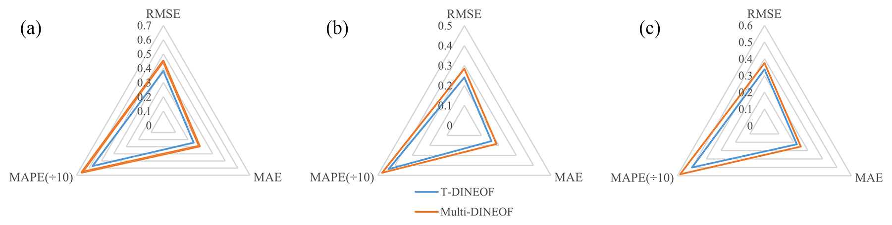
Figure 13 Radar charts of statistical accuracies for subregions 1–3 (a–c). The blue and red polygons represent T-DINEOF and Multi-DINEOF, respectively.

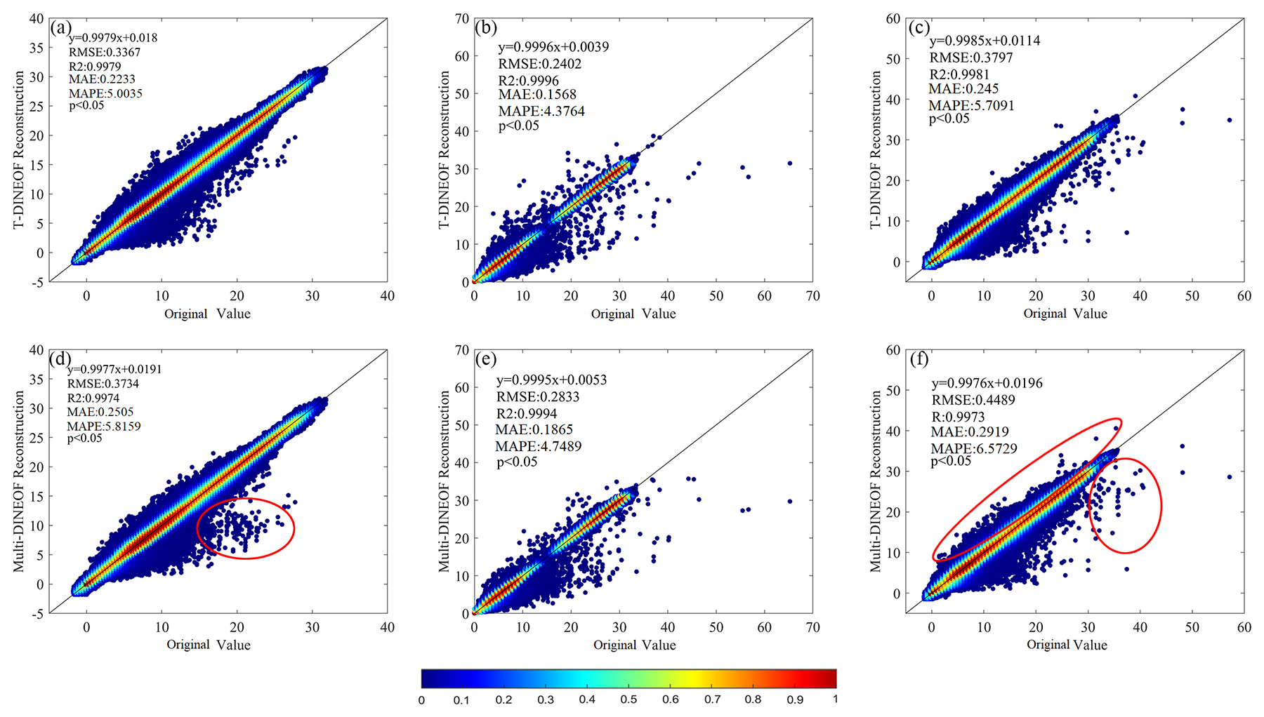
Figure 14 Scatter density plots for SST, SCHL, and SSW in subregions 1–3 (from left to right), obtained from (a–c) T-DINEOF and (d–f) Multi-DINEOF. Values are shown in their original physical units after inverse max-min normalization, using the parameters provided in Table 1: SST in °C, SCHL in mg m⁻³, and SSW in m s⁻¹.

Compared to subregion 3, the accuracy differences between T-DINEOF and Multi-DINEOF are more pronounced in subregion 1. Specifically, compared to Multi-DINEOF, T-DINEOF improves RMSE by 15.4 %, MAE by 16.1 %, and MAPE by 13.1 % in subregion 1, while improving RMSE by 9.8 %, MAE by 10.9 %, and MAPE by 14.0 % in subregion 3. Since the proportion of missing values in subregion 1 is higher than in subregion 3 (as shown in Fig. 2a), it can be inferred that T-DINEOF is more suitable for regions with a high proportion of missing values compared to Multi-DINEOF. The difference may be attributed to the structural designs of the Multi-DINEOF and T-DINEOF approaches. Multi-DINEOF reshapes all spatiotemporal variables into a single two-dimensional matrix, making its reconstruction accuracy more susceptible to degradation when the proportion of missing values is high. In contrast, the tensor structure of T-DINEOF distributes missing data across the third dimension, thereby mitigating the adverse impact of high missing-value proportions.

As shown in Fig. 14, the scatter density plots for T-DINEOF and Multi-DINEOF in all three subregions are mostly concentrated around the 1:1 line, with the slopes of the fitting lines exceeding 0.99, indicating the effectiveness of both methods in these subregions. Additionally, by comparing the scatter density plots, it can be observed that, similar to the results from the radar charts, the plots for both methods are comparable in subregion 2, despite T-DINEOF having slightly better accuracy. In subregions 1 and 3, however, Multi-DINEOF tends to produce some overestimated or underestimated values (red ellipses in Fig. 14d and f), which may account for its lower accuracy.

The reconstruction accuracies for each ocean variable across the three subregions are analyzed separately. Given the significantly larger range of MAPE values for the SCHL data compared to the corresponding RMSE and MAE values, enlarged versions of the RMSE and MAE plots are included in the corresponding accuracy charts. As shown in Fig. 15a–c, for SST data, although the accuracy differences among the three methods are consistent across different subregions, T-DINEOF achieves better accuracies than both Multi-DINEOF and Single-DINEOF in all subregions. Subregion 2, the equatorial region, shows better reconstruction accuracy than the mid-latitudes, with lower RMSE and MAE values. Subregion 1 exhibits higher RMSE and MAE but a lower MAPE compared to subregion 3. As shown in Fig. 2b, the proportion of missing SST data is significantly lower in the equatorial region than in the mid-latitudes, providing more information for data imputation and resulting in higher reconstruction accuracy.

As shown in Fig. 15d–f, for SCHL data, the differences in reconstruction accuracies among the three methods are minimal in subregion 2. However, in subregions 1 and 3, T-DINEOF achieves superior accuracy, particularly in subregion 3. Figure 2c shows that subregion 3 has the highest proportion of missing SCHL data, suggesting that T-DINEOF performs better in areas with a higher proportion of missing values.

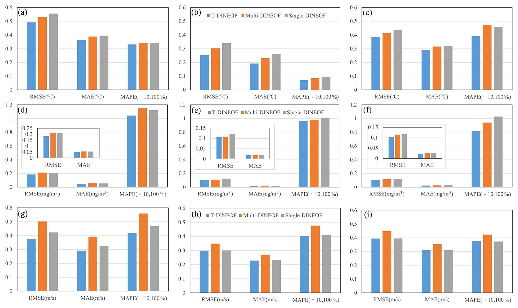
Figure 15 Statistical accuracies for (a–c) SST, (d–f) SCHL, and (g–i) SSW in subregions 1–3 (from left to right).

As shown in Fig. 15g–i, the trend in SSW reconstruction accuracy is consistent across all three subregions: Multi-DINEOF exhibits the lowest accuracy, followed by Single-DINEOF, with T-DINEOF achieving the highest accuracy. The accuracy differences are most pronounced in subregion 1, while in subregions 2 and 3, T-DINEOF slightly outperforms Single-DINEOF. According to Fig. 2d, subregion 1 has the highest proportion of missing SSW data, further highlighting T-DINEOF's advantage in regions with a high proportion of missing values.

We also selected daily L3 mapped MODIS Aqua SST and SCHL data, along with daily L3 AMSR2 SSW data from January to March 2022, to assess the effectiveness of the T-DINEOF method in reconstructing daily datasets with high missing-data proportions. As shown in Fig. S1, despite the missing-data ratio exceeding 78 % in all three subregions, T-DINEOF still outperforms Multi-DINEOF for the daily datasets, consistent with the results obtained for the monthly data. This conclusion further confirms the robustness of the T-DINEOF method and its effectiveness in reconstructing datasets with a high proportion of missing values. It is also important to note that the RMSE values reported in this study were computed using only the existing pixels. Consequently, when the missing-data ratio is high, the reduced number of pixels available for the calculation may result in an underestimation of the RMSE.

Figure 16 shows the temporal RMSE distributions for the three oceanic variables across different subregions during the experimental period. As illustrated in Fig. 16a–c, the RMSE variations for SST in subregion 2 are relatively small, indicating more stable reconstruction performance, while subregion 1 shows the greatest RMSE variation. In subregion 2, T-DINEOF (blue line) consistently achieves the lowest RMSE values during most periods, particularly in October 2017, September 2018, and August 2020. Despite not always having the lowest RMSE in subregions 1 and 3, T-DINEOF exhibits the least variation, highlighting its stable performance. Single-DINEOF (green line) shows significant fluctuations, achieving the lowest RMSE in some months but reflecting overall instability and lower accuracy. Multi-DINEOF, although more stable than Single-DINEOF, still trends higher in RMSE compared to T-DINEOF.

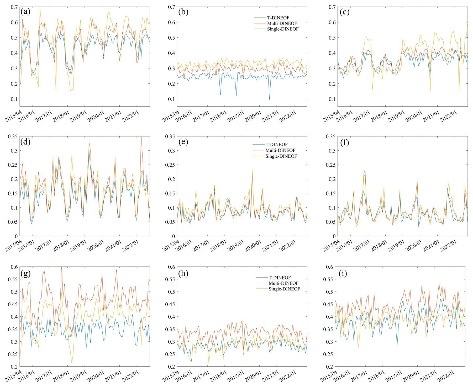
Figure 16 Temporal RMSEs for (a–c) SST, (d–f) SCHL, and (g–i) SSW in subregions 1–3 (from left to right).

As shown in Fig. 16d–f, for SCHL data, the RMSE values for T-DINEOF are slightly lower than those for Multi-DINEOF, with both showing similar RMSE distributions across subregions. Single-DINEOF occasionally shows higher RMSE, indicating poorer reconstruction accuracy. Generally, in subregion 1 (the mid-latitude regions in the Northern Hemisphere), the RMSE values exhibit pronounced fluctuations and follow a periodic pattern, with lower RMSE values in winter and higher in summer. The periodic RMSE variations observed in subregion 1 may be associated with the homogeneity of the SCHL data. During winter, subregion 1 exhibits lower standard deviation (SD) values (Fig. S2), indicating higher SCHL homogeneity. Generally, more homogeneous regions tend to exhibit lower reconstruction errors. Conversely, in summer, higher SD values reflect greater variability in SCHL, leading to correspondingly larger reconstruction errors. In subregion 3, the RMSE also shows a certain degree of periodic variation; however, compared with subregion 1, its RMSE values lack a clear periodic pattern. This finding is consistent with the relatively small SD values of subregion 3 shown in Fig. S1. In subregion 2, RMSE variations are smaller and exhibit no apparent regularity. In addition, taking the T-DINEOF method as an example, the correlation coefficients between RMSE and SD of log(SCHL) across the three subregions were calculated. In subregion 1, the correlation coefficient reaches 0.65, indicating that the pronounced periodic variations in SCHL significantly influence the variations in reconstruction accuracy. In contrast, in subregion 3, the smaller periodic variations in SCHL are only weakly correlated with changes in reconstruction accuracy (correlation $=-\mathrm{0.14}$), and in subregion 2, due to the relatively small SD values reflecting high SCHL homogeneity, the correlation between SD and RMSE is negligible (correlation =0.02).

For SSW data, as illustrated in Fig. 16g–i, the RMSE values are generally lower in subregion 2 (the equatorial region) compared to the mid-latitudes. Multi-DINEOF consistently shows higher RMSE values across all subregions, especially in subregion 1, indicating poorer performance in SSW reconstruction. Single-DINEOF occasionally achieves lower RMSE, but its values fluctuate more and are generally higher than those for T-DINEOF, which demonstrates greater stability and lower RMSE.

Since T-DINEOF, Multi-DINEOF, and Single-DINEOF all perform reconstruction on the entire spatiotemporal dataset, no clear relationship can be found between the missing data proportion of individual scenes and their corresponding reconstruction accuracy (not shown in manuscript).

Meanwhile, the monthly RMSEs of SST, SCHL, and SSW across different subregions were further evaluated (Fig. S3). The results show that, for SST, T-DINEOF achieves the highest reconstruction accuracy in most cases, with particularly notable improvements in subregion 2. Only in subregion 1 during January to March does the reconstruction accuracy of T-DINEOF appear slightly lower than that of Multi-DINEOF. For SCHL, in subregion 1, T-DINEOF achieves the best reconstruction accuracy in most months. In subregion 2, the reconstruction accuracy of T-DINEOF is slightly higher than that of Multi-DINEOF in most months, while Single-DINEOF yields the lowest accuracy. In subregion 3, T-DINEOF shows higher accuracy from October to the following February, whereas from May to September, its reconstruction accuracy is lower than that of both Multi-DINEOF and Single-DINEOF. For SSW, in subregion 1, T-DINEOF demonstrates higher accuracy in most months except from April to June. In subregion 2, T-DINEOF outperforms both Multi-DINEOF and Single-DINEOF in most months. In subregion 3, T-DINEOF achieves higher reconstruction accuracy from October to the following February and in April, while in the remaining months, Single-DINEOF performs better than T-DINEOF. It is also noteworthy that Multi-DINEOF exhibits the lowest accuracy for SSW. As discussed in Sect. 4.1, the correlation between SSW and the other variables (SST and SCHL) is relatively low. Therefore, the multivariate synergy in Multi-DINEOF does not enhance the reconstruction accuracy of SSW under low-correlation conditions. This also demonstrates that the T-DINEOF method, owing to its tensor-based reconstruction framework, is more effective in improving the reconstruction accuracy of variables with weak inter-variable correlations.

5 Discussion

The current multivariate DINEOF method essentially performs matrix-based reconstruction, which cannot fully utilize correlations between variables. With the development of third-order tensor research, there has been growing interest in the decomposition and reconstruction of third-order tensor. A T-DINEOF model based on the T-SVD technique was proposed in this study to better explore the relationships among multivariable data. Multiple accuracy metrics demonstrate that T-DINEOF outperforms the conventional Multi-DINEOF method both globally and across various subregions, indicating the superiority of third-order tensor reconstruction over matrix-based reconstruction. In addition, the proportion of missing data significantly impacts reconstruction accuracy. The experiments confirm that T-DINEOF shows a more substantial improvement in accuracy for regions with a high proportion of missing values. Furthermore, the correlations among different oceanic variables also affect reconstruction accuracy, with better performance observed when reconstructing multiple highly correlated variables together compared to reconstructing each variable individually. In addition, the statistical results demonstrate that even when data correlation is low, T-DINEOF still improves the reconstruction accuracy of the relevant oceanic variables. This improvement arises from performing tensor decomposition in a high-dimensional space (space × time × variable), which allows T-DINEOF to exploit cross-dimensional dependencies and capture coherent spatial–temporal patterns shared across variables. Consequently, the model can more effectively reconstruct low-correlation variables, as their spatial and temporal structures remain embedded within the overall tensor framework.

Although T-DINEOF outperforms the original DINEOF and Multi-DINEOF methods, it still relies on a single global optimal mode, which may not be ideal for capturing heterogeneous local dynamics within the study area or achieving the best reconstruction in specific regions and during intermediate iterations. Therefore, integrating improvements from original DINEOF methods and their variants into third-order tensor reconstruction is necessary. Furthermore, this study uses monthly oceanic variables, so temporal correlations are not considered. If daily or weekly data were used, incorporating temporal correlations among various oceanic variables would be essential for enhancing reconstruction accuracy. Additionally, compared to monthly data, daily or weekly datasets typically exhibit higher proportions of missing values. In this study, we demonstrated that T-DINEOF outperforms both Multi-DINEOF and Single-DINEOF in regions with high missing data proportions, suggesting that it may be more advantageous for reconstructing daily or weekly data (Fig. S2). However, due to the tensor operations involved, T-DINEOF requires longer computation times to reconstruct the same region. This may limit its application to larger-scale tensors, such as longer time-series images (91 scenes were used in this study) or tensors with more dimensions (three variables in this study). It is evident that, over the same time span, the volume of daily or weekly data is significantly greater than that of monthly data. Given the substantial data volume inherent in a third-order tensor, optimizing computational processes and accelerating processing speeds are crucial for the effective application of T-DINEOF to high-temporal-resolution datasets. Moreover, to unify MODIS SST and SCHL (high resolution) with AMSR2 SSW (low resolution), the nearest-neighbor method was used to downscale MODIS data to the AMSR2 resolution. Upscaling low-resolution data is an ill-posed nonlinear system problem that may introduce larger errors, whereas downscaling helps reduce error propagation. Therefore, MODIS SST and SCHL data were downscaled to the AMSR2 resolution rather than upscaling AMSR2 data to match the MODIS resolution. However, although the nearest-neighbor method is widely used for downscaling high-resolution imagery, it may still introduce artifacts that affect the reconstruction process. Consequently, adopting more advanced resampling techniques or using multi-source datasets with consistent spatial resolution could further improve reconstruction accuracy. Finally, it should be noted that if the source datasets contain systematic biases, such errors may be propagated through the reconstruction process, potentially affecting the accuracy of the final results. In particular, tensor-based methods may be more susceptible to such bias propagation, as errors in one variable can influence others through the coupled decomposition.

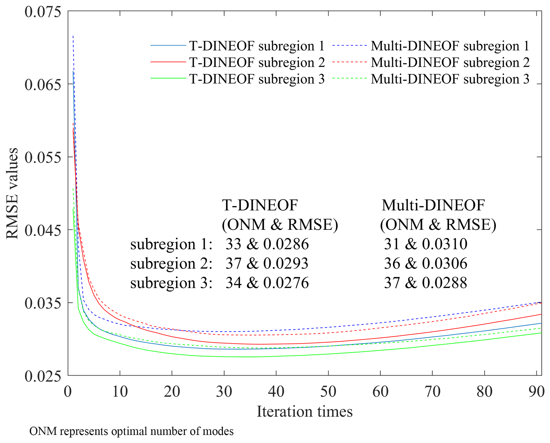
Figure 17 Distributions of RMSE values at the cross-validation pixels for T-DINEOF and Multi-DINEOF across three subregions during the iterative process.

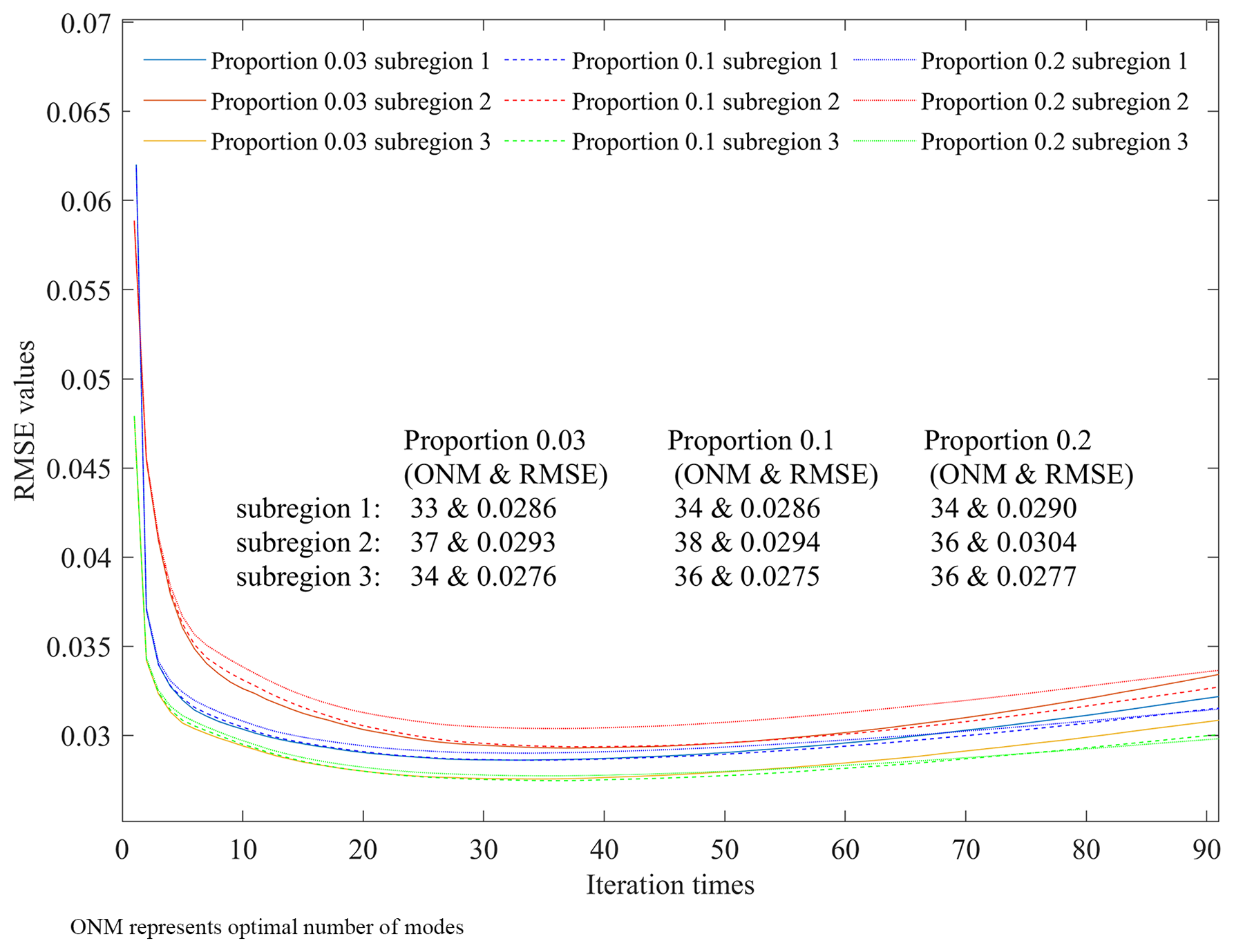
Figure 18 Distributions of RMSE values for T-DINEOF with cross-validation point proportions of 0.03, 0.1, and 0.2 across three subregions during the iterative process.

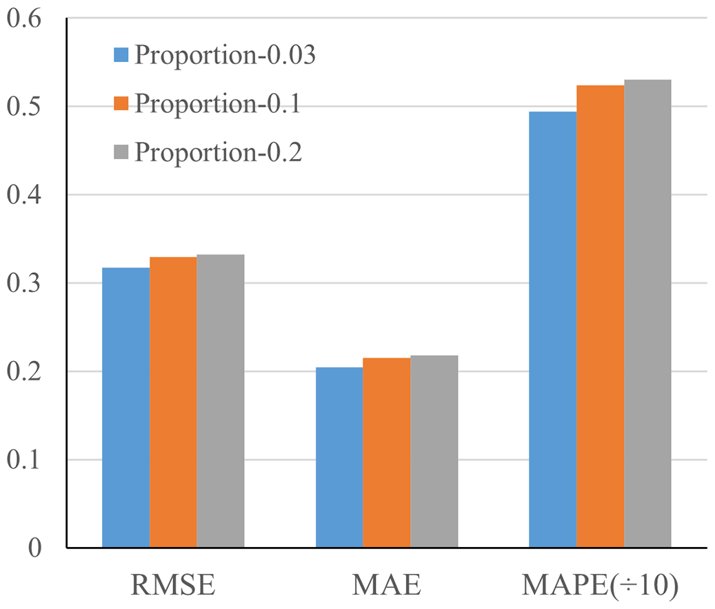
Figure 19 Bar chart of global statistical accuracies. The blue, red, and green bars represent T-DINEOF with cross-validation point proportions of 0.03, 0.1, and 0.2, respectively.

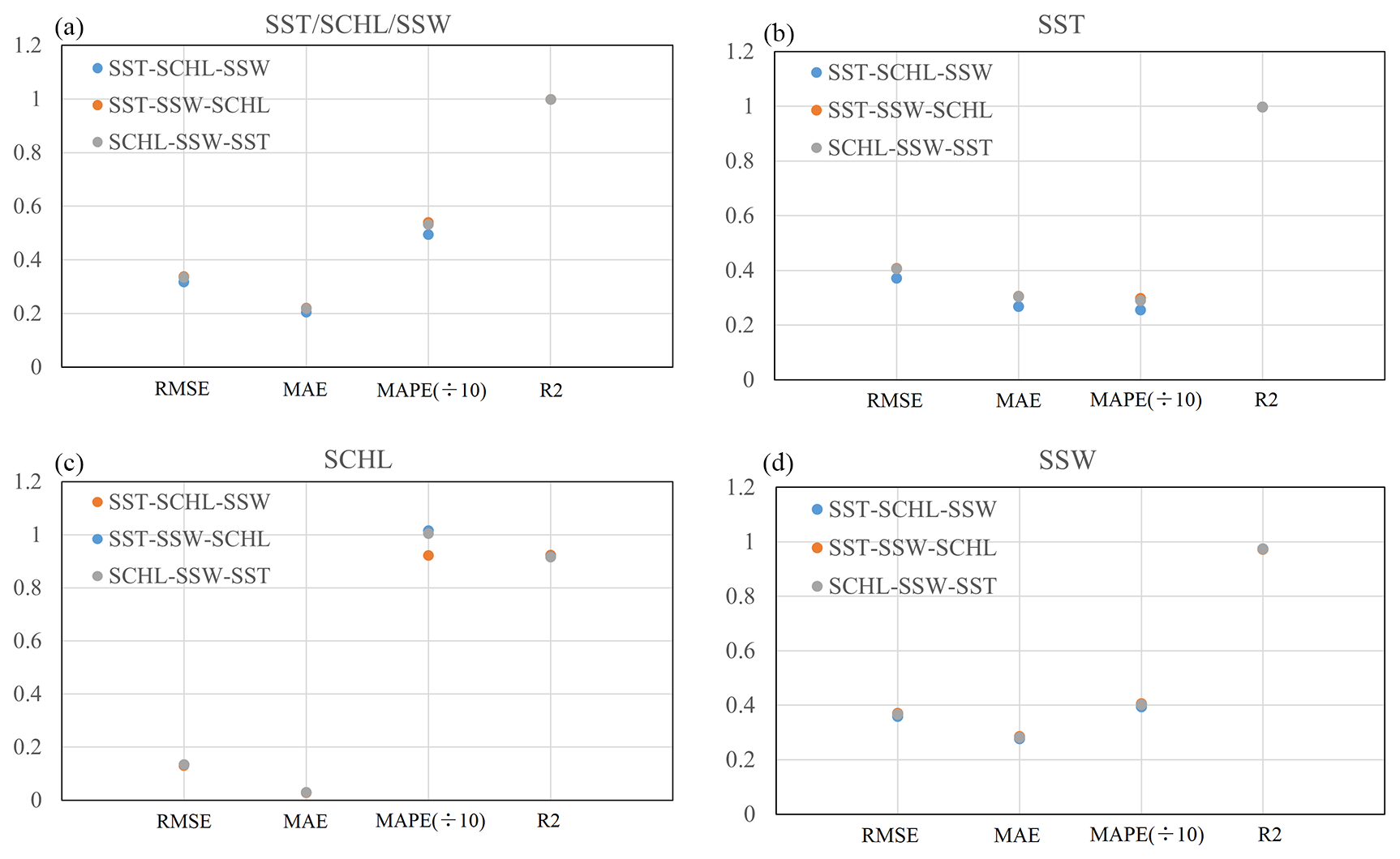
Figure 20 Differences in accuracies from different input orders for (a) the three oceanic variables, (b) SST, (c) SCHL and (d) SSW.

The optimal number of modes is an essential parameter for both T-DINEOF and Multi-DINEOF, typically determined by the smallest RMSE value at the cross-validation pixels during the iterative process. As shown in Fig. 17, during the iterative process, the RMSE distributions from the cross-validation pixels for T-DINEOF in the three subregions are lower than those for Multi-DINEOF, indicating superior reconstruction performance by T-DINEOF. In these three subregions, the optimal number of modes for T-DINEOF is 33, 37, and 34, respectively, compared to 31, 36, and 37 for Multi-DINEOF. The similarity in the optimal number of modes suggests that both methods converge after a similar number of iterations, but T-DINEOF consistently achieves lower RMSE values. In both the original DINEOF and Multi-DINEOF methods, 3 % of existing pixels are randomly selected as cross-validation pixels to determine the optimal number of modes. In this study, we individually selected 3 %, 10 % and 20 % of the existing pixels as the cross-validation pixels to analyze the impact of different proportions of cross-validation pixels on T-DINEOF. As shown in Fig. 18, the RMSE distributions for different proportions of cross-validation pixels are similar across the three subregions. The optimal numbers of modes and the corresponding RMSE values obtained from these varying proportions show only minor differences. This suggests that the proportion of cross-validation pixels has a negligible impact on determining the optimal number of modes for T-DINEOF. Since cross-validation pixels are considered as missing values in the process of determining the optimal number of modes, the fact that T-DINEOF yields similar optimal numbers of modes and corresponding RMSE values across different proportions of cross-validation pixels indicates its stability in handling varying amounts of missing data.

The global reconstruction accuracies of the T-DINEOF model under different proportions of cross-validation pixels are illustrated in Fig. 19. Overall, the accuracies obtained under the three proportions are quite similar, while the 3 % proportion yields relatively lower error values. This suggests that the proportion of cross-validation pixels has a minimal impact on the reconstruction accuracy of the T-DINEOF model. Therefore, consistent with the conventional DINEOF method, 3 % of the existing pixels were randomly selected as the cross-validation pixels in this study.

In this study, the order of the oceanic variables in the input third-order tensor, specifically, the third dimension, was SST–SCHL–SSW. To analyze the impact of variable ordering on T-DINEOF, two alternative input orders, SST–SSW–SCHL and SCHL–SSW–SST, were randomly selected for comparative analysis. As shown in Fig. 20, the reconstruction accuracies for SST, SCHL, and SSW, as well as for each individual oceanic variable, are similar across the different input orders, particularly for the SCHL and SSW data. For SST data, the order of input variables has a minor impact, with an average RMSE difference of 0.04 °C. Among the three selected input orders, the configuration that yields the best reconstruction performance is the SST–SCHL–SSW order. Since the T-DINEOF method is built on a tensor reconstruction framework, it simultaneously optimizes multiple variables during the reconstruction process, and the order of input variables has minimal effect on reconstruction accuracy, which is one of the method's key advantages.

Finally, the proposed T-DINEOF method, with its capability to reconstruct missing values in multi-dimensional spatiotemporal datasets, has broad applications beyond oceanography. In numerical weather prediction, it can fill gaps in key variables such as SST and SSW, improving data completeness and forecast accuracy by preserving inter-variable correlations. During natural disasters – such as hurricanes or harmful algal blooms – it helps restore data lost due to cloud cover or sensor failure, enabling more accurate real-time monitoring and timely emergency response. In marine biodiversity research, T-DINEOF ensures the continuity of datasets like SST and SCHL, which are critical for tracking ecological changes and assessing climate impacts. Additionally, in fisheries and aquaculture, reconstructed environmental baselines support stock assessments, site selection, and early detection of stressors such as hypoxia, thereby promoting sustainable resource management. Future research will focus on the following directions: achieving locally optimal reconstruction within the third-order tensor and refining the iterative process of the T-DINEOF model to further enhance its performance; integrating temporal autocorrelations among multiple oceanic variables into the tensor reconstruction framework to more comprehensively capture the dynamic coupling of oceanic parameters; and improving computational efficiency to enable large-scale, high spatiotemporal resolution reconstruction and applications of multiple oceanic variables.

6 Conclusions

This study proposed the T-DINEOF model, which leverages the T-SVD technique for multivariable data reconstruction, aiming to improve the accuracy of multiple oceanic variables reconstruction. In comparison to the Multi-DINEOF and original DINEOF methods, which rely on matrix-based reconstruction, T-DINEOF demonstrates superior accuracy for both overall and individual oceanic variables. This indicates that third-order tensor reconstruction more effectively utilizes the correlations among multiple oceanic variables, thus enhancing reconstruction performance. Additionally, T-DINEOF is particularly well-suited for regions with a high proportion of missing values, showing significant accuracy improvements. Even though the input SSW exhibits low correlation with SST and CHL, the T-DINEOF method is still able to achieve high-accuracy reconstruction of the SSW field.

Both T-DINEOF and Multi-DINEOF converge with a similar number of iterations; however, T-DINEOF achieves higher accuracy at convergence. Various proportions of cross-validation pixels yield similar optimal numbers of modes and corresponding RMSE values, suggesting that the proportion of cross-validation pixels does not significantly impact the T-DINEOF model. Additionally, the order of multiple oceanic variables in the third-order tensor has a minimal effect on the T-DINEOF model.

The T-DINEOF model represents a novel approach for reconstructing multiple oceanic variables. However, attaining local optimal reconstruction within the third-order tensor and optimizing the iterative process of the T-DINEOF model are crucial for further enhancing its performance. Additionally, integrating temporal correlations among multiple oceanic variables into the tensor reconstruction process requires further research. Furthermore, improving computational efficiency is essential for the large-scale reconstruction of multiple oceanic variables. One potential approach is to use machine learning methods (e.g., Random Forests, XGBoost, or neural networks) for the initial estimation of missing values, followed by the application of the T-DINEOF method for further refinement, thereby improving the algorithm's efficiency. Lastly, the effectiveness of the T-DINEOF method in reconstructing other types of datasets, such as sea surface salinity, and reanalysis products, will also be evaluated in future research.