A multidecadal sea level rise and its hiatus in the tropical Atlantic margin off northwest Africa

Satellite and reanalysis data sets are analyzed to explain sea level changes in the tropical North Atlantic margin off northwest Africa. The study domain sea level was rising as far back as 1986 and a pause in sea level rise (hiatus) began around 2010 and stopped in 2019. Characteristics of sea level anomaly and its drivers during a period of rise (1996–2004) and the hiatus period (2010–2018) are analyzed and compared. Results show that the most effective cause of domain-wide sea level rise during the period of rise is seawater expansion owing to changes in density structure (steric expansion), with almost equal contribution from temperature-driven (thermosteric) expansion and salinity-driven (halosteric) expansion. The cause of the domain-wide pause in sea level rise is a large thermosteric contraction that counteracted halosteric expansion and mass accumulation. Multidecadal sea level increase, defined here as the difference between the mean sea level during the period of rise and the hiatus period, is owing to steric expansion, vertical land motion, and mass accumulation, which contributed 56 %, 24 %, and 16 %, respectively. There are, however, regional differences in the patterns of multidecadal steric and mass adjustment. In the northern subdomain where ocean processes predominate mass-driven sea level variability, the steric adjustment is dominated by halosteric expansion, whereas in the southern subdomain where atmosphere-ocean processes predominate mass-driven sea level variability, the steric adjustment is dominated by thermosteric expansion. The accumulation of low-salinity water in the northern subdomain and precipitation in the southern subdomain appears to be associated with a mutual adjustment of vertical and horizontal velocity distribution inside the domain and west of it in the area of the Guinea Dome, a permanent upwelling region where isotherms are displaced upwards. The low-salinity water influx to the northern subdomain is linked to changes in the southward-flowing Canary Current. A probable hypothesis inferred from correlation and potential vorticity analysis is that the Canary Current source region was freshened by currents that supply water to the region via two pathways: an open ocean path that is consistent with the Azores Current, and a Western Europe coastal ocean path that is consistent with the Portugal Current and Portugal Coastal Current system. The results obtained highlight a multidecadal linkage between sea level anomalies in the eastern tropical North Atlantic margin and salinity anomalies elsewhere in the North Atlantic.

1 Introduction

It is useful to specify the physical linkages between climatic events occurring in ocean margins and elsewhere in the ocean. Understanding the operating phenomena that accomplish these long-term linkages provides predictive power to anticipate adverse coastal change following events that have already occurred elsewhere in the ocean. More than 40 % of the world's population reside within 150 km of the coast (Reimann et al., 2023; United Nations, 2018) and seafood from coastal marine ecosystems supplies about 15 % of the protein consumed by this population (Sumaila et al., 2011). Another important reason for characterizing events in ocean margins is that fluctuations in coastal seawater properties express shifts in the heat and water fluxes that maintain the prevailing regional climate (Robinson and Brink, 2006). Analyzing satellite measurements of these fluctuations thus offers an approach to elucidate processes of coastal climate change.

Sea level fluctuations in the eastern tropical Atlantic margin off northwest Africa (hereafter “domain,” Fig. 1) is important for climate change investigations because it reflects changes in several elements of the global ocean and atmosphere circulation (Stramma et al., 2005). These elements include the northeasterly trade wind and its continental branch, the northeasterly Harmattan wind; the southeasterly Monsoon; the south-flowing Canary Current that supplies feed-water to the North Equatorial Current; the north and south branches of the North Equatorial Countercurrent that bifurcates near the African coast (Ibrahim and Sun, 2022); and the so-called “Guinea Dome,” a region off the African coast with permanent upward flux of cool water from beneath that causes doming (i.e. upward displacement) of isotherms (Fig. 12). Moreover, because of persistent upwelling of nutrient-rich waters in large subregions of this domain, it is one of the three most productive marine ecosystems in the global ocean (Chavez, 2012). The complex interaction of these elements promotes considerable interannual variability (Ibrahim and Sun, 2022) as shown in the deseasonalized time series of ocean and atmosphere quantities in the domain (Figs. 2 and 4).

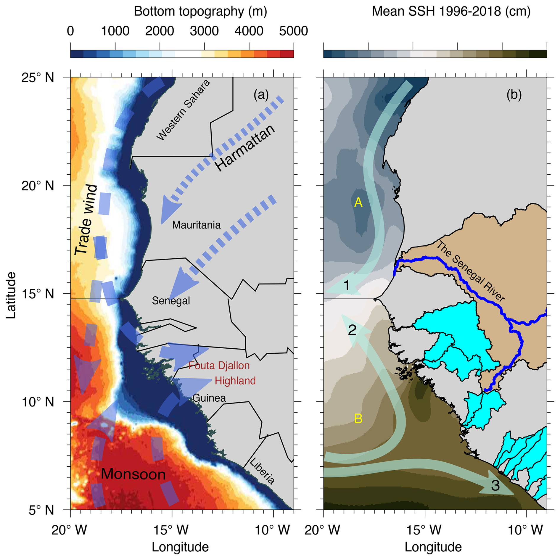
Figure 1 Characteristics of the eastern tropical Atlantic margin off northwest Africa (domain). (a) Bottom topography (GEBCO, 2021), and the mean annual spatial pattern of the three dominant atmosphere wind systems in the region (indicated in blue dash lines): trade wind, Harmattan wind, and monsoon wind. (b) Multi-year (1996–2018) mean annual sea-surface height (SSH) (C3S Climate Data Store, 2018), and the three dominant ocean current systems in the region (indicated in solid cyan lines): (1) the Canary Current, and the (2) north and (3) south branches of the bifurcated North Equatorial Countercurrent, respectively; capital letters A and B denote the two analysis subdomains identified from EOF analysis (Sect. 2.3). The Canary Current traverses subdomain A (14.75–25° N, 9–20° W.), and the north branch of the bifurcated North Equatorial Countercurrent traverses subdomain B (5–14.75° N, 9–20° W) (Ibrahim and Sun, 2022). The regions colored in tan and cyan over land are the catchments of the rivers that discharge into subdomains A and B, respectively. See Sect. 2.2 for more details.

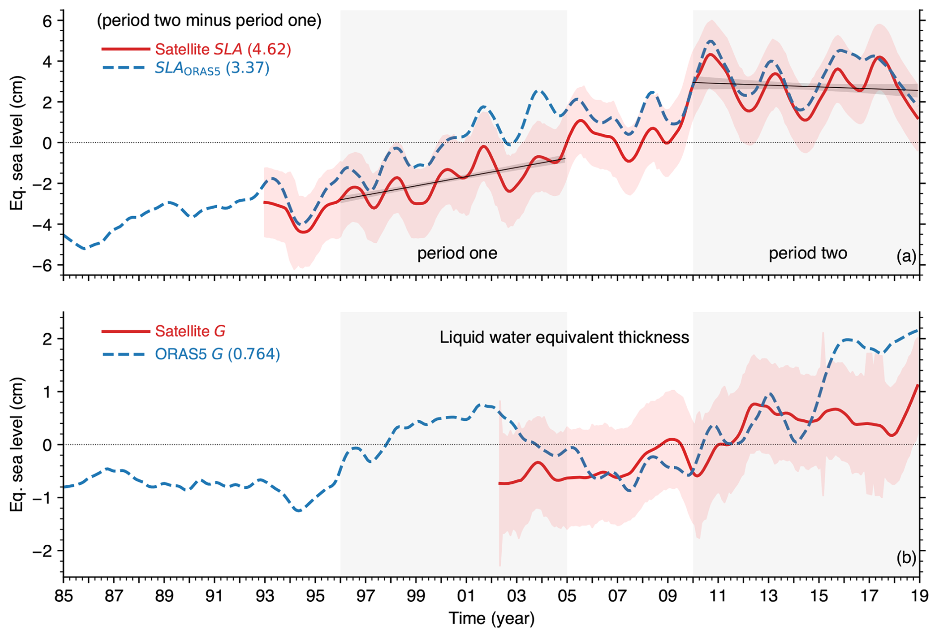
Figure 2 Area-average monthly time series of domain characteristics (mean annual cycle removed, i.e. the long-term mean of each month is subtracted from the monthly datasets). The numbers in parenthesis are the multi-year mean difference. In this and subsequent figures, the lightly shaded background represent period one and two, respectively. (a) Satellite altimetry sea level anomaly (SLA) (red solid line) and measurement error (lightly shaded red region): regression line (black solid line) and 95 % confidence interval (gray region around each line) for each period; and ORAS5 SLA (SLA_ORAS5) (blue dash line); for comparison, period one and two mean difference of satellite altimetry global average sea level is 4.02 cm. (b) GRACE satellite (see Sect. 2.1) ocean mass change (G) (red solid line) and calculated ORAS5 G (blue dash line) (see Sect. 2.2). GRACE G missing months (about 10 % of the data set) have been infilled with the climatology of the missing month. A 13-month low-pass (moving average) filter is applied to all the time series to attenuate high-frequency fluctuations; the lightly shaded red region is the GRACE measurement uncertainty (NASA, Jet Propulsion Laboratory, 20121).

The domain sea-surface temperature increased in 1995 (Ibrahim and Sun, 2022). However, changepoint analysis (Lanzante, 1996) of the domain satellite altimetry measurement (Pujol et al., 2016; C3S Climate Data Store, 2018) shows a hiatus in sea level rise between two change points in 2010 and in 2019 (Fig. 2a). Since the 2019 change point, the domain sea level has started rising again (not shown). The satellite record of sea level anomaly (SLA) is relatively short, thus, to determine the trend pattern prior to the start of satellite altimetry in 1993, we used the European Centre for Medium-Range Weather Forecasts (ECMWF) Ocean Reanalysis System 5 (hereafter “ORAS5”, see Sect. 2.2) to also calculate the SLA trend (Zuo et al., 2019). ORAS5 SLA (SLA_ORAS5) and satellite altimeter SLA trend patterns are consistent during the overlap period (1993–2018), and SLA_ORAS5 shows that the sea level there was rising as far back as 1986 (Fig. 2a).

Here our aim is to characterize the evolution of the sea level and its drivers during a multi-year period of rising sea level (the rising state, period one: 1996–2004) and pause in the sea level rise (the hiatus state, period two: 2010–2018). To do this, we focus on two sea level characteristics and performed two related tasks. First, to differentiate the dominant drivers during the rising and hiatus states, we analyze the sea level displacement during each period. The objective of task one is to explain what caused the rising sea level in period one and what caused the sea level rise to pause in period two. Second, we analyze the increase in sea level between period one and two. The objective of task two is to explain why the mean sea level is relatively higher in period two compared to period one. Another way to describe these two tasks is that task one gives insight into the mechanism of short-term sea-level changes, while task two gives insight into the mechanism of long-term (multidecadal) sea level changes. This analysis approach is useful because the causes of sea-level fluctuation (Sect. 2.1) operate at many timescales, from a few days to many decades. Moreover, sea level characteristics over short periods, say ten years, are very important for coastal infrastructure planning, design, and investments (Cane, 2010; Lawton and Kershaw, 2025).

We chose period one because it overlaps with the satellite altimetry era and in order to avoid the transition period when sea level fluctuations can be comparatively unstable owing to large variations in heat and water fluxes (Ibrahim et al., 2020). We chose period two in order to assess the sea level drivers during the hiatus state. The explanation of the observed SLA trend must account for the steric, mass and atmospheric pressure shifts between period one and two, since these are the three factors that control SLA fluctuations. Moreover, because the atmospheric pressure effect is comparatively small in general, we anticipate that steric and mass changes play the key roles in the observed sea level fluctuation pattern.

To achieve this aim we first performed an empirical orthogonal function analysis of the domain SLA, which revealed two subregions (denoted “subdomain A” and “subdomain B” in Fig. 1b) with differing horizontal pattern of SLA variability (Sect. 2.3). This is followed by separating the multi-year mean SLA change in each subdomain into its constituent steric, mass and atmospheric pressure changes, thus identifying the drivers of sea level change in each subdomain (Sect. 3). Two key aspects of the dynamical chain of events are discussed in Sects. 4 and 5, respectively, and our conclusions are in Sect. 6.

2 Methods of analysis

To understand and characterize the measured domain SLA pattern (Fig. 2a), it is necessary to analyze the causes of change in the vertical displacement of the free ocean surface at each instant. The dominant causes have been known long ago and illustrated by several authors (Pattullo et al., 1955; Gill and Niller, 1973; Pinardi et al., 2014; Fukumori and Wang, 2013; Ibrahim and Sun, 2020). However, owing to the diversity of terminology in the sea level literature (Gregory et al., 2019), we briefly summarize these causes (Sect. 2.1) to facilitate interpretation of our results. This is followed by a description of the data sets that we used to calculate the change in these causes (Sect. 2.2) and the results of EOF analysis that reveal two subdomains with differing pattern of SLA variability (Sect. 2.3). Note that in Sect. 2.1 we refer to SLA_ORAS5 and ORAS5 G, which are both calculated using the ORAS5 reanalysis data sets that are described in Sect. 2.2.

2.1 The causes of sea level fluctuation

The basic formulation of the physics of sea level fluctuation given by Gill and Niller (1973) is followed closely here and is thus referred to for completeness. Introducing η (λ,ϕ) for the free ocean surface, where λ and ϕ are longitude and latitude (positive northward and eastward), respectively; H (m) for the seabed distance (i.e. depth from the mean ocean surface); ρ (kg m⁻³) for seawater density; p_b ($\mathrm{kg}{\mathrm{m}}^{-\mathrm{1}{\mathrm{s}}^{-\mathrm{2}}}$) for ocean bottom pressure; p_a ($\mathrm{kg}{\mathrm{m}}^{-\mathrm{1}}{\mathrm{s}}^{-\mathrm{2}}$) for atmospheric pressure at the ocean surface, g (m s⁻²) for the constant acceleration due to gravity, and γ (m) for the vertical land motion; then based on the hydrostatic relation the variation of the free ocean surface from its time-mean, η^′ (m), can be approximated by Gill and Niller (1973)

$$\begin{array}{}\text{(1)}& {\displaystyle }{\displaystyle }\underset{\text{SLA}}{\underbrace{{\mathit{\eta }}^{\prime }}}=\underset{{\text{SLA}}_{\text{ORAS5}}}{\underbrace{\underset{Z_{\mathit{\alpha }}}{\underbrace{\left(-{\displaystyle \frac{\mathrm{1}}{{\mathit{\rho }}_{\mathrm{o}}}}\underset{-H}{\overset{\mathrm{0}}{\int }}{\mathit{\rho }}^{\prime }\mathrm{d}z\right)}}+\underset{G}{\underbrace{{\displaystyle \frac{p_{\mathrm{b}}^{\prime }}{g{\mathit{\rho }}_{\mathrm{o}}}}}}}}+\underset{{\mathit{\zeta }}_{\mathrm{a}}}{\underbrace{\left({\displaystyle \frac{-p_{\mathrm{a}}^{\prime }}{g{\mathit{\rho }}_{\mathrm{o}}}}\right)}}+\mathit{\gamma }\end{array}$$

where ρ^′, $p_{\mathrm{a}}^{\prime }$, $p_{\mathrm{b}}^{\prime }$ are the variations of ρ, p_a, and p_b from their time-mean, respectively, and ρ_o is a representative density (a constant). The mean sea level is defined as the geopotential surface z=0 where the time average fluctuation of η is equal to zero (Apel, 1987). Equation (1) states that η^′, the sea level anomaly from its time-mean, hereafter SLA (cm), is caused by: (1) changes in density structure resulting in expansion/contraction of the seawater column, i.e. steric fluctuation, hereafter Z_α (cm); (2) variations in freshwater and salt mass (which determines weight and therefore pressure at the ocean bottom) inside the seawater column below the ocean surface, hereafter G (cm); and (3) variation in atmospheric pressure at the ocean surface, hereafter ζ_a (cm). Note that in the first and third term on the right-hand side of Eq. (1), a negative variation (i.e. ${\mathit{\rho }}^{\prime }<\mathrm{0}$, or $p_a^{\prime }<\mathrm{0}$) implies an increase in SLA, and vice versa.

For consistency, because satellite SLA trend pattern and ocean reanalysis SLA_ORAS5 trend pattern are in agreement (Fig. 2a), we used SLA_ORAS5 to evaluate Eq. (1). However, satellite SLA (Fig. 2a) is corrected for ζ_a (i.e. barometric correction), but SLA_ORAS5 does not include atmospheric pressure forcing and vertical land motion (Zuo et al., 2019), i.e. SLA_ORAS5 is the sum of Z_α and G as shown in Eq. (1). Since our aim is to specify the contribution of the four causes on the right side of Eq. (1) to the SLA shift, we therefore estimate and add ζ_a and γ to SLA_ORAS5. Hence, hereafter, SLA refers to SLA_ORAS5 plus ζ_a and γ. Compared to Z_α and G, the contribution of ζ_a to SLA shifts is relatively small, so we use the approximation suggested by Gill and Niller (1973), p_a change of 1 mbar corresponds to η^′ change of 1 cm, which is consistent with direct calculations using term three on the right side of Eq. (1) and taking ρ_o=1025 kg m⁻³.

ORAS5 is a Boussinesq model, meaning that it conserves volume but not mass. Greatbatch (1994) showed that requiring the conservation of mass in Boussinesq ocean models introduces two new terms in Eq. (1): the first term is weak and can be neglected, while the second term corresponds to the global inverse barometer effect, i.e. a spatially uniform net rate of expansion/contraction of the global sea level. Therefore, we calculate and include this second component, hereafter referred to as the “Boussinesq correction (ε),” in our analysis, i.e. ε is added to the right-hand side of Eq. (1). However, for the sake of simplicity of description and because the contribution of ε is small in this study domain (less than 1 % of the SLA increase, see Table B1), we do not write it in Eq. (1).

We used two methods to estimate Z_α. In method one we used ORAS5 reanalysis temperature and salinity to calculate G (ORAS5 G, see details in the next section); we then used ORAS5 G and SLA_ORAS5, together with Eq. (1), to obtain Z_α as a residual. Method one may be thought of as subtracting GRACE measurement from altimetry measurement. In method two we directly calculate Z_α, as well as its temperature-driven component (thermosteric change, hereafter Z_t) and salinity-driven component (halosteric change, hereafter Z_s), using the numerical formulation of Tabata et al. (1986) which is given in pressure coordinates by

$$\begin{array}{}\text{(2a)}& {\displaystyle }& {\displaystyle }{Z}_{\mathit{\alpha }}={\displaystyle \frac{\mathrm{1}}{g}}\underset{p_{\mathrm{a}}}{\overset{p_{\mathrm{b}}}{\int }}\left(\mathrm{\Delta }\mathit{\alpha }\right)\mathrm{d}p\text{(2b)}& {\displaystyle }& {\displaystyle }{Z}_{\mathrm{t}}={\displaystyle \frac{\mathrm{1}}{g}}\underset{p_{\mathrm{a}}}{\overset{p_{\mathrm{b}}}{\int }}\left({\displaystyle \frac{\partial \mathit{\alpha }}{\partial T}}\right)\mathrm{\Delta }T\mathrm{d}p\text{(2c)}& {\displaystyle }& {\displaystyle }{Z}_{\mathrm{s}}={\displaystyle \frac{\mathrm{1}}{g}}\underset{p_{\mathrm{a}}}{\overset{p_{\mathrm{b}}}{\int }}\left({\displaystyle \frac{\partial \mathit{\alpha }}{\partial S}}\right)\mathrm{\Delta }S\mathrm{d}p\end{array}$$

where α (m³ kg⁻¹) is the specific volume; T (°C) is temperature, S (g kg⁻¹) is salinity; $\mathrm{\Delta }T=T-\overline{T}$ and $\mathrm{\Delta }S=S-\overline{S}$ represent the mean monthly departure of T and S from their respective climatological annual means ($\overline{T}$ and $\overline{S}$); Δα is the departure of specific volume corresponding to small values of ΔT and ΔS; and the integration is carried out between pressure levels from the ocean surface to the seabed. Figure 5 shows the comparison of Z_α obtained from method one and two and the agreement between them is good, which gives us confidence in our calculations. One source of error in Eq. (2) is that, because we neglect higher order derivatives in the estimation of the thermal expansion coefficient ($\partial \mathit{\alpha }/\partial T$) and haline contraction coefficient ($\partial \mathit{\alpha }/\partial S$), Eq. (2) may not capture high frequency steric fluctuations. However, because our focus here is on long-term low frequency SLA fluctuations, this error is unlikely to affect our results.

The satellite Gravity Recovery and Climate Experiment (GRACE) data set provides monthly estimates of G at 1° spatial resolution (Save et al., 2016; Save, 2020), but the record is short (March 2002 to October 2017) and it has many time gaps. To overcome this deficiency we used ORAS5 G (see calculation details in the next section). Figure 2b shows that ORAS5 G captures the GRACE G trend pattern, which gives us confidence in our calculations.

It is also possible to estimate G from its constituent components. Introducing P (cm) for precipitation averaged over the domain, E (cm) for evaporation averaged over the domain, R (cm) for land runoff into the domain, and F_net (cm) for seawater net flux through the domain boundaries, then G is given by

$$\begin{array}{}\text{(3)}& {\displaystyle }{\displaystyle }G=P-E+R+F_{\text{net}}.\end{array}$$

In reality, however, it is difficult to calculate F_net in Eq. (3) from ocean reanalysis data sets by calculating the fluxes through the domain boundaries because ORAS5 and most ocean reanalysis systems do not conserve mass. Therefore, because local salinity and temperature (e.g. from Argo floats) are assimilated into ORAS5, which enhances its reliability, we used the calculated ORAS5 G for the analysis here. By substituting this calculated G and the estimated P, E, and R into Eq. (3), we derived F_net as a residual.

In order to estimate vertical land motion (γ), the fourth term on the right-hand side of Eq. (1), we subtracted tidal gauge (which moves with the land) measurements (OBS), from the absolute dynamic topography (ADT) altimetry measurements: i.e. $\mathit{\gamma }=\text{ADT}-\text{OBS}$ (Wöppelmann and Marcos, 2016). Two tide gauge stations are within the study domain: station 1816: DAKAR 2 (17.42° W, 14.68° N), available from 1992 to 2018 (Permanent Service for Mean Sea Level, 2025a); and station 2036: NOUAKCHOTT (16.04° W, 17.99° N), available from 2007 to 2015 (Permanent Service for Mean Sea Level, 2025b). Station 2036, located in the north of the study domain, has a shorter record. Accordingly, using an inverse weighting approach to derive station weights (94 % weight for station 1816 and 6 % weight for station 2036), we calculated a weighted average from the two tide stations. We estimate the two period difference of γ to be 1.10 cm (Table B1), with a 95 % confidence interval of (0.232, 1.97 cm).

2.1.1 Metric for analyzing sea level and its drivers during the rising state and during the hiatus state

To find and explain what caused the sea level to continue rising during period one and what caused the sea level rise to pause during period two, we calculate the change in SLA and its drivers during period one and during period two. Introducing x for SLA or for its drivers and m_x,i (m month⁻¹) for the linear least-squares regression (trend) line slope of x during period i (period 1 or period 2, each having 108 months), the change in x ($\widehat{x}$) during each period i is given by

$$\begin{array}{}\text{(4)}& {\displaystyle }{\displaystyle }\widehat{x_i}=m_{x,i}\times \mathrm{108}.\end{array}$$

In the case of SLA, the quantity $\widehat{x}$ is the sea level displacement during each period.

2.1.2 Metric for analyzing the multidecadal change in sea level and its drivers

To explain the relatively higher mean SLA in period two compared to period one, we calculate the two period mean difference for SLA and for its drivers. Thus, if $\stackrel{\mathrm{‾}}{x_{P\mathrm{1}}}$ and $\stackrel{\mathrm{‾}}{x_{P\mathrm{2}}}$ are the period one and two means of x, respectively, the two period mean difference is $\stackrel{\mathrm{‾}}{x_{P\mathrm{2}}}$ minus $\stackrel{\mathrm{‾}}{x_{P\mathrm{1}}}$.

2.2 Data sets and processing

The altimeter SLA measurements that we used is the climate-oriented gridded, monthly, 0.25° horizontal resolution, Copernicus Climate Change Service satellite observations dataset version vDT2021, which is available from 1993 to present (C3S Climate Data Store, 2018). This satellite record is designed for monitoring the long-term evolution of sea level and other ocean and climate indicators, thus it is suitable for this study.

We obtained ocean reanalysis sea level anomaly (SLA_ORAS5), seawater salinity (S), seawater temperature (T), and zonal and meridional ocean current velocity from the monthly ECMWF ORAS5 ocean reanalysis data set (Zuo et al., 2019), which is available from 1979 to 2018. ORAS5 has 0.25° horizontal resolution and 75 vertical levels, and we downloaded it from the Integrated Climate Data Center, Hamburg University.

Notice the discrepancy between SLA and SLA_ORAS5 (Fig. 2a): this is likely because (1) observations near the coast that are assimilated into ORAS5 have larger errors in general, (2) ORAS5 does not assimilate altimeter SLA near the coast, and (3) vertical land displacement is not well represented in ORAS5 (Zuo et al., 2019). Compared to SLA, the period two minus period one SLA_ORAS5 difference for the domain and subdomains are about 5 % larger: this discrepancy is accounted for by the barometric and Boussinesq corrections (see Table B1). ORAS5 assimilates in situ and satellite measurements (S, T, and SLA), it uses information on the global mean sea level trend to close the fresh-water budget, and it includes a bias correction scheme for pressure in the tropical region and for salinity and temperature in the extra-tropical region (Zuo et al., 2019; Balmaseda et al., 2013). These ORAS5 characteristics are likely why SLA_ORAS5 long-term trend in this domain is in good agreement with altimeter SLA measurements (Fig. 2a). Overall, Carton et al. (2019) showed that ORAS5 is suitable for long-term variability studies and Ibrahim and Sun (2022) have verified ORAS5 ensemble control member (opa0), which we use here, in this domain. This gives us confidence that ORAS5 data set is suitable for this study.

To calculate ORAS5 G, first, we used ORAS5 S and T, together with the Gibbs SeaWater (GSW) Oceanographic Toolbox of TEOS-10 version 3.6.19 in Python, to obtain in situ density (kg m⁻³); second, using this density, together with ORAS5 layer thickness (m) and domain area (m²), we calculated mass (kg); third, using seawater density of 1025 kg m⁻³ and the domain area, we obtained mass in equivalent water thickness units (cm), the same units as GRACE data (Save et al., 2016). Note that ORAS5 does not assimilate GRACE. Accordingly, GRACE is an independent source to validate the calculations of ORAS5 G. The agreement between ORAS5 G and GRACE data is good (Fig. 2b). However, there are discrepancies, particularly during 2003–2005 and from 2015, which may be explained by degraded GRACE data when the satellite orbit is near exact repeat (July–December 2004, January–February 2015) and when altimetry measurements are taken from only one accelerometer, starting around August 2016 (NASA, Jet Propulsion Laboratory, 20121).

We estimated P minus E (PminusE) and ζ_a using the monthly ECMWF ERA5 atmospheric reanalysis surface data set (Hersbach et al., 2020), which is available from 1979 to present. ERA5 has 30 km spatial resolution and we downloaded it from the Copernicus Climate Change Service Climate Data Store (Hersbach et al., 2023). To estimate R we calculated PminusE over the catchment of the rivers that discharge into the domain (World Bank, 2019) (Fig. 1b). Compared to measured land runoff, this R is likely more accurate since it also includes coastal groundwater discharge into the domain. The large land area extending inland around 10° N (Fig. 1b) is the catchment of the Niger River, which has its headwaters in the Fouta Djallon Highland and flows inland. There are three other land areas near the coast, around 11, 13, and 15° N, that are unresolved in the rivers data set that we used (World Bank, 2019), probably because these areas have no gauged rivers. In general, river contribution to SLA increase is comparatively small (Fig. 4d).

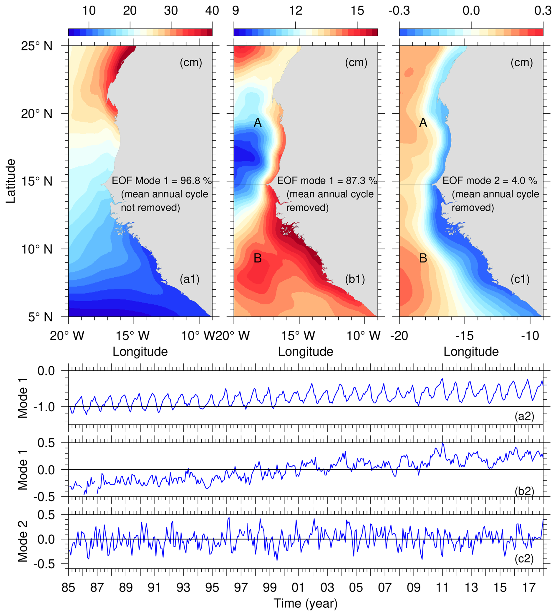
Figure 3 Empirical Orthogonal Function (EOF) analysis of the domain monthly SLA. (a1) Mode 1 with mean annual cycle retained. (b1) Mode 1 with mean annual cycle removed. (c1) Mode 2 with mean annual cycle removed. (a2–c2) (a1), (b1), and (c1) time series, respectively.

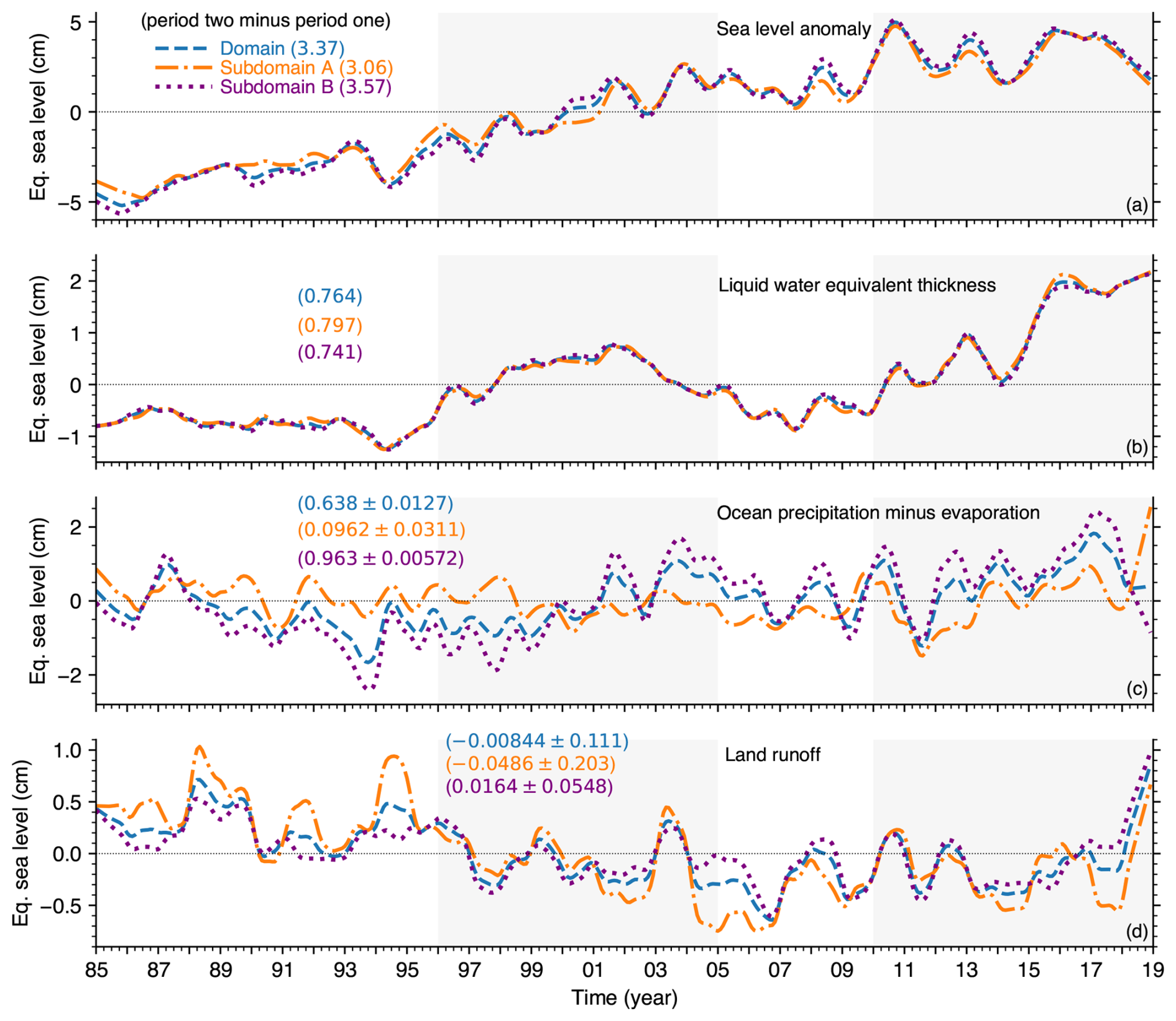
Figure 4 Monthly time series (mean annual cycle removed) of domain and subdomain characteristics, and multi-year mean change (i.e. period two minus period one) in parenthesis. (a) Area-averaged SLA_ORAS5 in the domain (blue dash line), subdomain A (orange dash-dotted line), and subdomain B (purple dotted line). (b) ORAS5 G, curves are as in (a). (c) ERA5 precipitation minus evaporation (PminusE) over the ocean, curves are as in (a). (d) ERA5-derived land runoff, curves are as in (a). A 13-month low-pass (moving average) filter is applied to all the time series.

2.3 Analysis subdomains

As a first step to comparing the causes of the change in SLA trend pattern between period one and two, we carried out an empirical orthogonal function (EOF) analysis of SLA in the domain to identify coherent horizontal structures (Fig. 3). This is useful to ensure correct spatial averaging of atmosphere and ocean variables for time series analysis. Figure 3a1 and a2 are the spatial pattern and time series of EOF mode 1 with the mean annual cycle retained, which enable reconstruction of the whole pattern of variability during 1985–2017: the temporal pattern shows an annual variability and a long-term steadily rising SLA (Fig. 3a2).

EOF analysis mode 1 with the mean annual cycle removed explains more than 87 % of the temporal-horizontal variance and it reveals two subregions with differing spatial patterns of SLA variability (Fig. 3b1), which are hereafter denoted “subdomain A” and “subdomain B” as shown in Fig. 3b1 and c1. EOF mode 1 with the mean annual cycle removed accounts for a large proportion of the total variance (87.3 %), indicating that the spatial structure of SLA variation revealed in mode 1 is stable (Fig. 3b1). EOF mode 2 with the mean annual cycle removed accounts for only 4 % of the temporal-horizontal variance (Fig. 3c1). The horizontal pattern of mode 1 indicates a large SLA difference (greater than 24 cm) between subdomains A and B Fig. 3b1.

The boundary between subdomain A and B (Fig. 3b1) is around the 14.75° N line of latitude, at the western tip of the African continent near Dakar, Senegal (Fig. 1). Subdomain A and B correspond to regions of comparatively shallow and deep bathymetry (Fig. 1a) as well as to regions of comparatively low and high mean sea surface height (Fig. 1b), respectively. Based on this EOF analysis, we analyze the causes of the change in SLA pattern in each subdomain between period one and two.

3 Changes in the causes of sea level fluctuation

To find and explain what caused the rising sea level in period one and what caused the sea level rise to pause in period two, in Sect. 3.1 we describe the contribution of the two dominant causes of sea level fluctuations, steric and mass changes (Eq. 1), during period one and two. To find and explain what caused the relatively higher sea level in period two compared to period one, in Sect. 3.2 we describe the relative contributions of all the causes of sea level fluctuation. In Sect. 3.3, we characterize the dominant driver of the multidecadal increase in sea level.

3.1 Contributions of steric and mass changes during the rising state and during the hiatus state

Table A1 gives the change in SLA and its drivers during period one and two. The barometric, Boussinesq, and vertical land motion terms (Eq. 1) are unlikely to change much during each period (9 years), so we do not include these terms in Table A1.

A striking result for the whole domain that may explain the rising sea level in period one and the hiatus in period two is the change in sign and magnitude of the total steric component (Z_t+Z_s) of the sea level displacement, from a positive contribution (3.67 cm) in period one to a negative contribution (−2.84 cm) in period two (Table A1). Because the mass contribution (G) to the sea level displacement is positive in period one and two, implying that G causes the sea level to rise, the rising sea level in period one is therefore caused by the positive contribution from both the total steric and mass components, while the pause in seal level rise in period two (the hiatus state) is owing to the negative contribution from the total steric component. This result also holds for subdomain A and B.

The halosteric part (Z_s) of the total steric contribution to domain-wide sea level displacement is positive in period one and two, but the thermosteric part (Z_t) is positive in period one and negative in period two (Table A1). This means that the switch from a rising sea level in period one to the hiatus in period two is owing to domain-wide cooling in period two.

However, compared to period one, the domain-wide halosteric contribution is smaller in period two, implying increase in salt content. In subdomain A, the halosteric contribution is positive in period one and two, but stronger in period two (implying decrease in salt content); and in subdomain B, the halosteric contribution is positive in period one and negative in period two (Table A1). Therefore, the weaker domain-wide halosteric contribution during period two is because of increase in subdomain B salt content. In general the magnitude of the halosteric change in subdomain A is substantially larger than in subdomain B.

In period one, the main drivers of the rising sea level in subdomain A are mainly the halosteric contribution and the mass contribution, accounting for about 92 % and 6 %, respectively, of subdomain A sea level displacement. In subdomain B, the main drivers of the rising sea level in period one are the thermosteric contribution, the halosteric contribution, and the mass contribution, accounting for about 71.5 %, 19.4 %, and 5.7 %, respectively, of subdomain B sea level displacement. Moreover, the positive ocean transport contribution is the main cause of the mass contribution in subdomain A, but the positive P−E contribution is the main cause of the mass contribution in subdomain B (Table A1).

In period two, the main driver of the pause in sea level rise in subdomain A is the large negative thermosteric contribution that overcomes the sum of positive contributions from the halosteric contribution and the mass contribution. In subdomain B, the main drivers of the pause in sea level rise are the negative thermosteric contribution and a comparatively small negative halosteric contribution, which together overcomes the positive mass contribution (Table A1).

The picture that emerges from these results is that the domain-wide sea level rise in period one is mainly caused by nearly equal thermosteric and halosteric expansion, and a comparatively small contribution from mass gain. The pause in sea-level rise in period two is because of substantial cooling, resulting in a large thermosteric contraction that counterbalanced the sea-level rise owing to halosteric expansion and mass gain. The origin of this cooling is unclear. A heat balance analysis that compares the heat gains and losses to the domain during period one and two is necessary to explain its mechanism.

3.2 Contribution of sea level drivers to the multidecadal increase in sea level

The two period difference (i.e. period two minus period one) of the area-average multi-year mean SLA and the factors that causes it to change are given in Table B1. Here we summarize the percentage contributions. Using the residual calculation approach based on Eq. (1), Z_α, γ, G, and ζ_a contributed about 56.5 %, 23.9 %, 16.5 %, and 2.71 %, respectively, to the multi-year mean SLA increase in the whole domain (Table B1). This same pattern of contributions (Z_α is dominant, followed by γ, G, and ζ_a) is shown in subdomain A and B, with slightly differing magnitudes compared to the whole domain.

The temporal pattern of the residual Z_α (Eq. 1) and the calculated Z_α (Eq. 2) are almost identical (Fig. 5). The small discrepancy between them is likely because, unlike the calculated Z_α, the change in ζ_a is included in the residual Z_α; and, as stated before, we neglect second and higher order Taylor expansion terms for the steric expansion/contraction coefficients in Eq. (2) (Tabata et al., 1986).

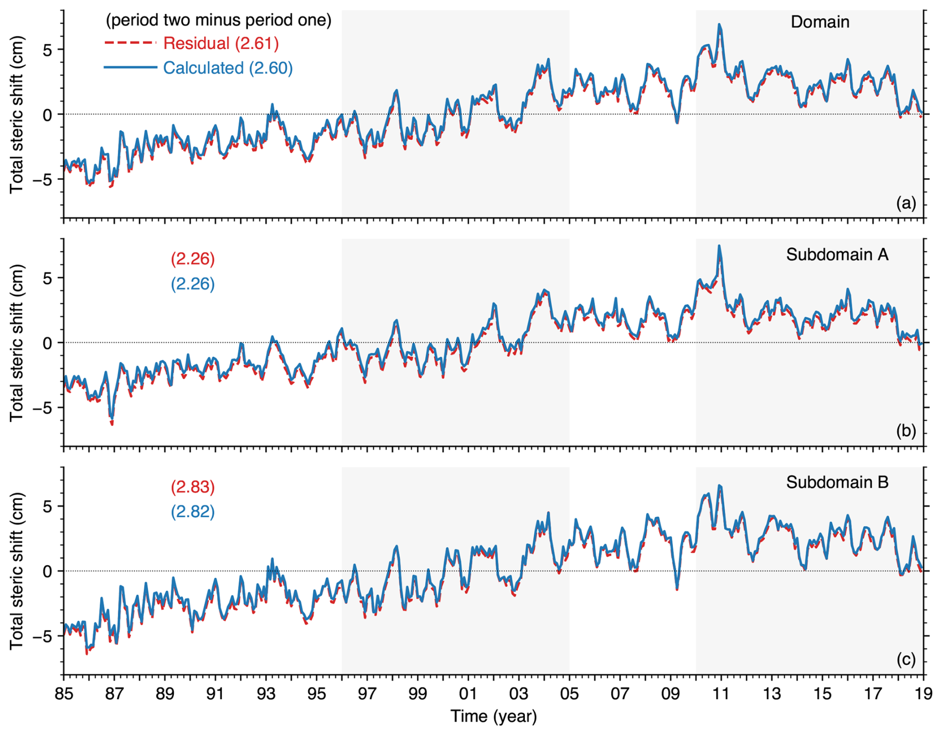
Figure 5 Comparison of total steric (Z_α) changes during 1985–2018 obtained with two different methods: in method one Z_α is obtained (red curve) as a residual using Eq. (1), i.e. SLA minus G, and in method two Z_α is directly calculated (blue curve) using Eq. (2). (a) Total steric shift in the domain obtained as a residual (red curve) and calculated (blue curve). (b) The same as (a) but for subdomain A. (c) The same as (a) but for subdomain B.

In the domain, subdomain A and subdomain B, PminusE contributed about 13.8 %, 2.22 %, and 20.1 % (Ibrahim and Sun, 2023) of the multi-year mean SLA increase, respectively; R contributed about −0.180 %, −1.12 %, and 0.340 %, respectively; and F_net contributed ≈2.90 %, 17.3 %, and −4.96 %, respectively, (Fig. 4c and d, Eq. 3, Table B1).

In summary (Table B1), neglecting γ which has the same value in the whole domain and the subdomains, the three dominant drivers of the multidecadal increase in sea level in the domain, in decreasing order of effect, are Z_α, PminusE and ζ_a; for subdomain A they are Z_α, F_net, and ζ_a; and for subdomain B they are Z_α, PminusE, and F_net. As expected, steric increase is the dominant driver of the observed sea-level variation pattern in the domain as well as in the two subdomains. The second dominant driver in subdomain A (F_net, 17.3 %) is different from the second dominant driver in subdomain B (PminusE, 20.1 %). Since F_net expresses mass exchange between ocean regions and PminusE expresses mass exchange between the ocean and the atmosphere, one interpretation of these results is that, with regards to mass effects on long-term SLA variability in this domain (i.e. G in Eq. 1), ocean processes predominate in subdomain A, while atmosphere-ocean processes predominate in subdomain B. This interpretation is consistent with the differing spatial pattern of SLA variability in subdomain A and subdomain B that is revealed in the EOF analysis mode 1 with the mean annual cycle removed (Fig. 3b1), which shows a low and high pattern of variability in large areas of subdomain A and B, respectively.

Note that, because F_net and PminusE modulate the domain temperature and salinity (and therefore the domain density), these two factors also contribute to the total steric change (Z_α). To characterize the mechanism of Z_α and show the operating processes, in the following section we compare the relative roles of temperature and salinity on Z_α.

3.3 Relative effect of temperature and salinity on the multidecadal increase in sea level

To assess the comparative roles of temperature and salinity on the multidecadal increase in subdomain A and B Z_α, and to specify the ocean current changes associated with the multidecadal shift in subdomains A and B F_net, we examined subdomains A and B vertical structure. Figure 6a1, b1, a2, and b2 show the T–S profile and T–S diagram, respectively, in subdomains A and B, averaged over periods one and two.

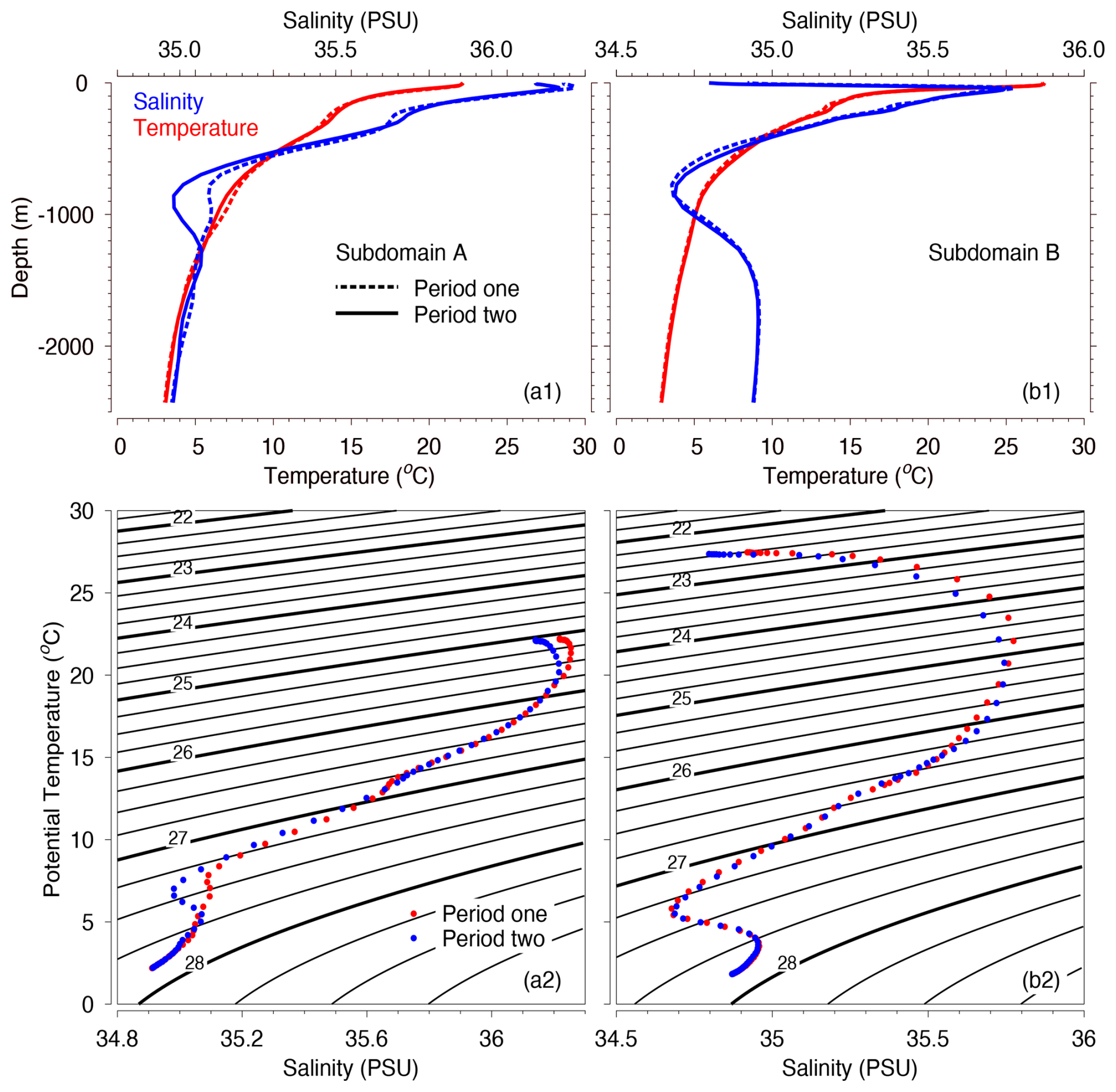
Figure 6 Multi-year mean vertical structure in the domain. (a1, b1) Period one (dotted line) and period two (solid line) T–S profile for subdomains A and B, respectively; salinity is shown in blue and temperature is shown in red. (a2, b2) Period one (red dotted line) and period two (blue dotted line) T–S diagram for subdomains A and B, respectively. Notice the large salinity change in (a1) and (a2).

In subdomain A, salinity and temperature decreased in the 0–1265 m depth range in period two (Fig. 6a1), especially in the 700–1265 m depth range. These changes are evident in the density profile which do not overlap for the two periods (Fig. 6a2). However, the slight decrease in density is not visible (Fig. 6a2), probably because decrease in salinity (which decreases density) and decrease in temperature (which increases density) have opposing effects on density. In subdomain B, near-surface salinity decreased during period two (Fig. 6b2), which confirms the multidecadal increase in subdomain B PminusE (Fig. 4c). The change in subdomain B density structure is mainly between surface and about 300 m (Fig. 6b2).

To further specify the changes in temperature and salinity temporal pattern at differing depths, we separated subdomains A and B into four vertical layers based on their salinity vertical profile (Fig. 7a1 and b1). Layer 1 is at depth 0–50 m, layer 2 is at depth 50–735 m, layer 3 is at depth 735–1725 m, and layer 4 is at depth 1725–5000 m.

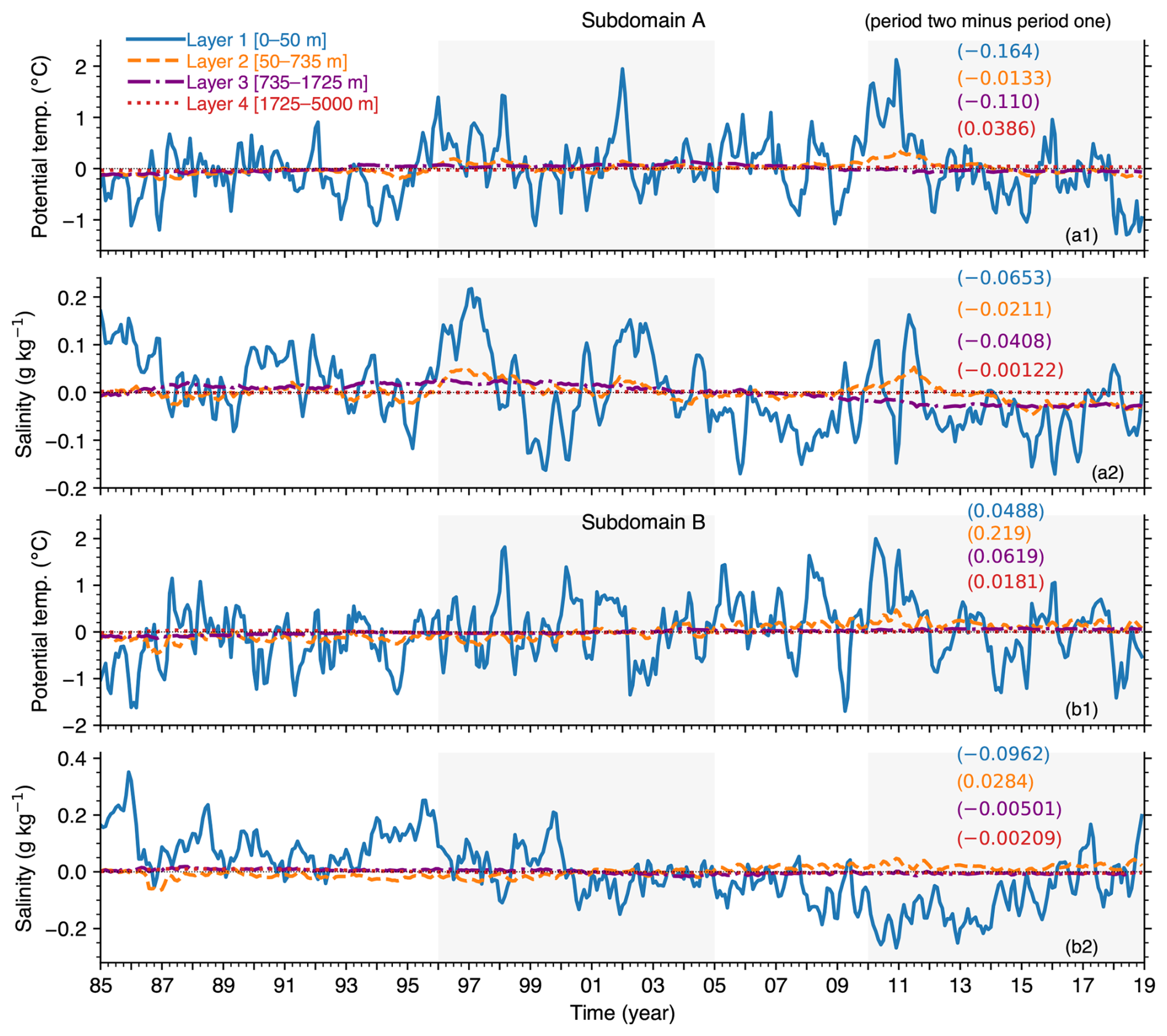
Figure 7 Monthly time series (mean annual cycle removed) of area-and-layer average ocean properties. (a1) Subdomain A potential temperature (temp.). (a2) Subdomain A salinity. (b1) Subdomain B potential temp. (b2) Subdomain B salinity. The numbers in parenthesis are period two minus period one values of temperature and salinity in each layer.

Figure 7 shows the layer-averaged monthly time series (mean annual cycle removed) of temperature and salinity in subdomain A and B, and the difference of the means for the two periods. Compared to period one, period two subdomain A layers 1–3 temperature decreased, while layer 4 temperature increased (Fig. 7a1), implying that only layer 4 thermosteric expansion contributed to the multi-year increase in subdomain A Z_α. Subdomain A layers 1–4 salinity decreased between periods one and two (Fig. 7a2), implying that halosteric expansion in the entire water column contributed to the multidecadal increase in subdomain A Z_α. Between periods one and two subdomain B layers 1–4 temperature increased (Fig. 7b1), implying that thermosteric expansion in all four layers contributed to the multidecadal increase in subdomain B Z_α. Compared to period one, period two subdomain B layer 2 salinity increased, while layers 1, 3, and 4 salinity decreased (Fig. 7b2), implying that layers 1, 3, and 4 halosteric expansion contributed to the multidecadal increase in subdomain B Z_α.

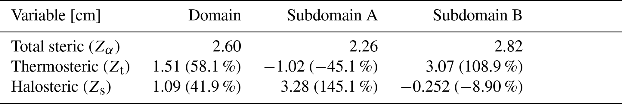
To ascertain the comparative role of temperature and salinity in subdomain A and B steric change, we calculated the thermosteric (Z_t) and halosteric (Z_s) shifts in each subdomain (Eq. 2b and 2c, Fig. 8). In the domain as a whole, Z_t is slightly larger than Z_s, 1.51 vs. 1.09 cm (Fig. 8), respectively. However, there are large differences between the two subdomains. In subdomain A, Z_t is $\approx -$1.02 cm and Z_s is ≈3.28 cm; while in subdomain B Z_t is ≈3.07 cm and Z_s is $\approx -$0.252 cm (Fig. 8). This means that in the domain, Z_t and Z_s contributed about 58 % and 42 %, respectively, of the total steric increase (Z_α) between period one and two; in subdomain A, Z_t and Z_s contributed about −45 % and 145 %, respectively, of Z_α; and in subdomain B Z_t and Z_s contributed about 109 % and −9 %, respectively, of Z_α. Therefore, halosteric expansion is the dominant driver of the multidecadal increase in subdomain A sea-level, while thermosteric expansion is the dominant driver in subdomain B. These results highlight the role of salt as an important driver of long-term regional sea-level shift, a role that is less recognized (compared to the role of heat) in discussions of sea-level changes under global climate change (Durack et al., 2014). Indeed, Ponte et al. (2021); Llovel and Lee (2015); Antonov et al. (2002) have suggested that changes in salinity affect SLA patterns in large areas of the world ocean at short and long timescales.

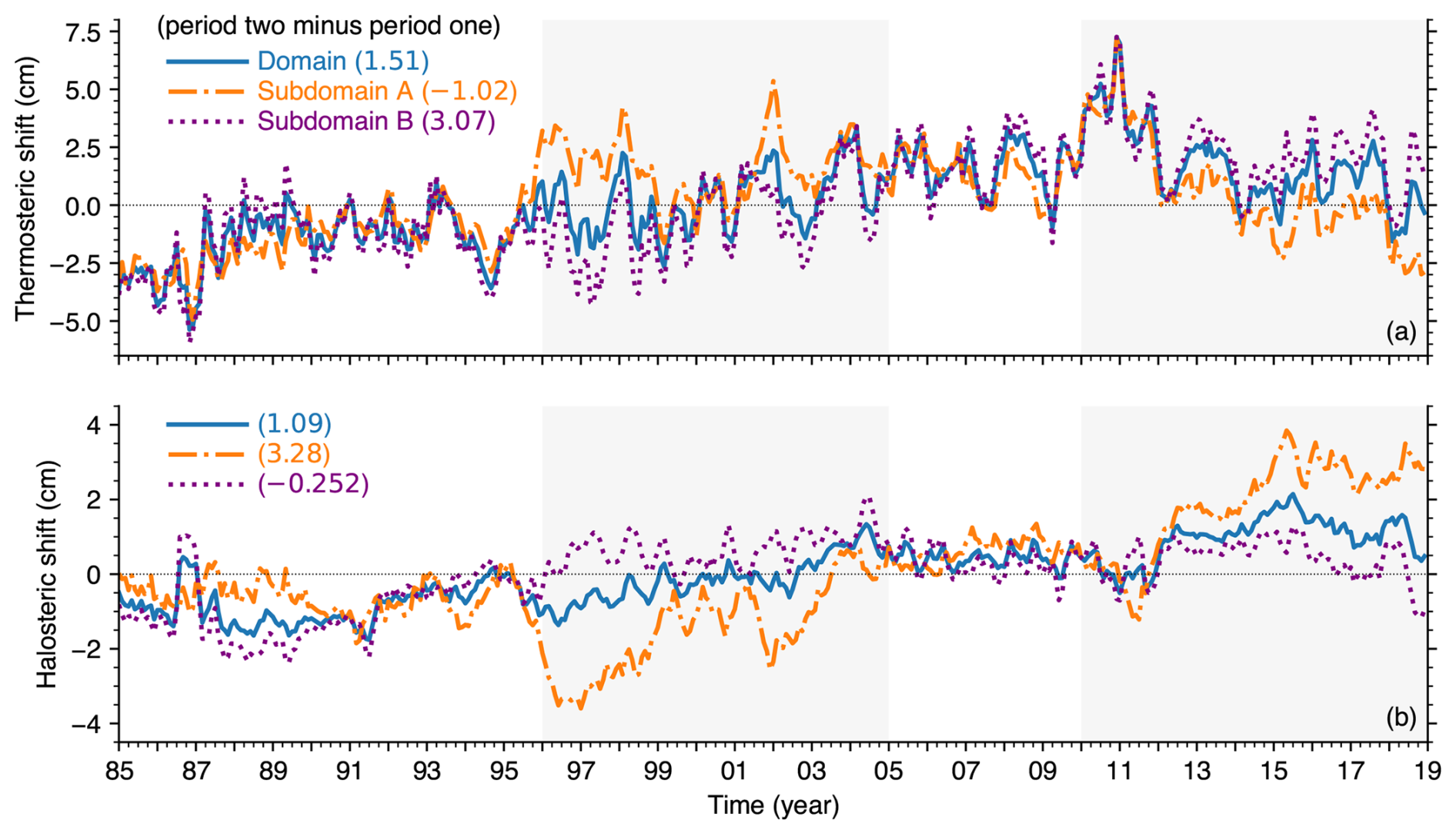
Figure 8 Monthly steric characteristics. (a) Area average thermosteric shifts in the domain (blue), subdomain A (orange) and subdomain B (purple). (b) Same as a but for halosteric shifts: notice the comparatively large multi-year halosteric increase in subdomain A. The time series are obtained from direct calculations using Eq. (2). The sum of (a) and (b) is the total steric shift, Z_α, which is given in Table B2.

It is beyond the scope of this work to analyze the domain heat and salt balance to find the physical processes that caused the thermosteric and halosteric shifts in subdomain A and B. Nonetheless, owing to three peculiarities of subdomain A that suggest the source of the freshening that caused the large halosteric increase there (145 %/3.28 cm, Table B2), we propose a plausible explanation for subdomain A freshening.

First, PminusE contributed only 2.22 %/0.0962 cm of subdomain A SLA increase, indicating that precipitation is not the key driver of the multidecadal freshening in subdomain A. Second, the multidecadal change in river runoff inside subdomain A is small ($-\mathrm{1.12}\mathrm{\%}/-\mathrm{0.0486}\mathrm{cm}$) and there is no river runoff north of it, indicating that freshwater from land is not the source of subdomain A freshening. Third, the Mediterranean Sea outflow at the Strait of Gibraltar north of subdomain A has a higher salinity than subdomain A (Fig. 9a1, b1, and c1) (Baringer and Price, 1997; Naranjo et al., 2017; Aldama-Campino and Döös, 2020), indicating that this outflow is not the cause of subdomain A freshening.

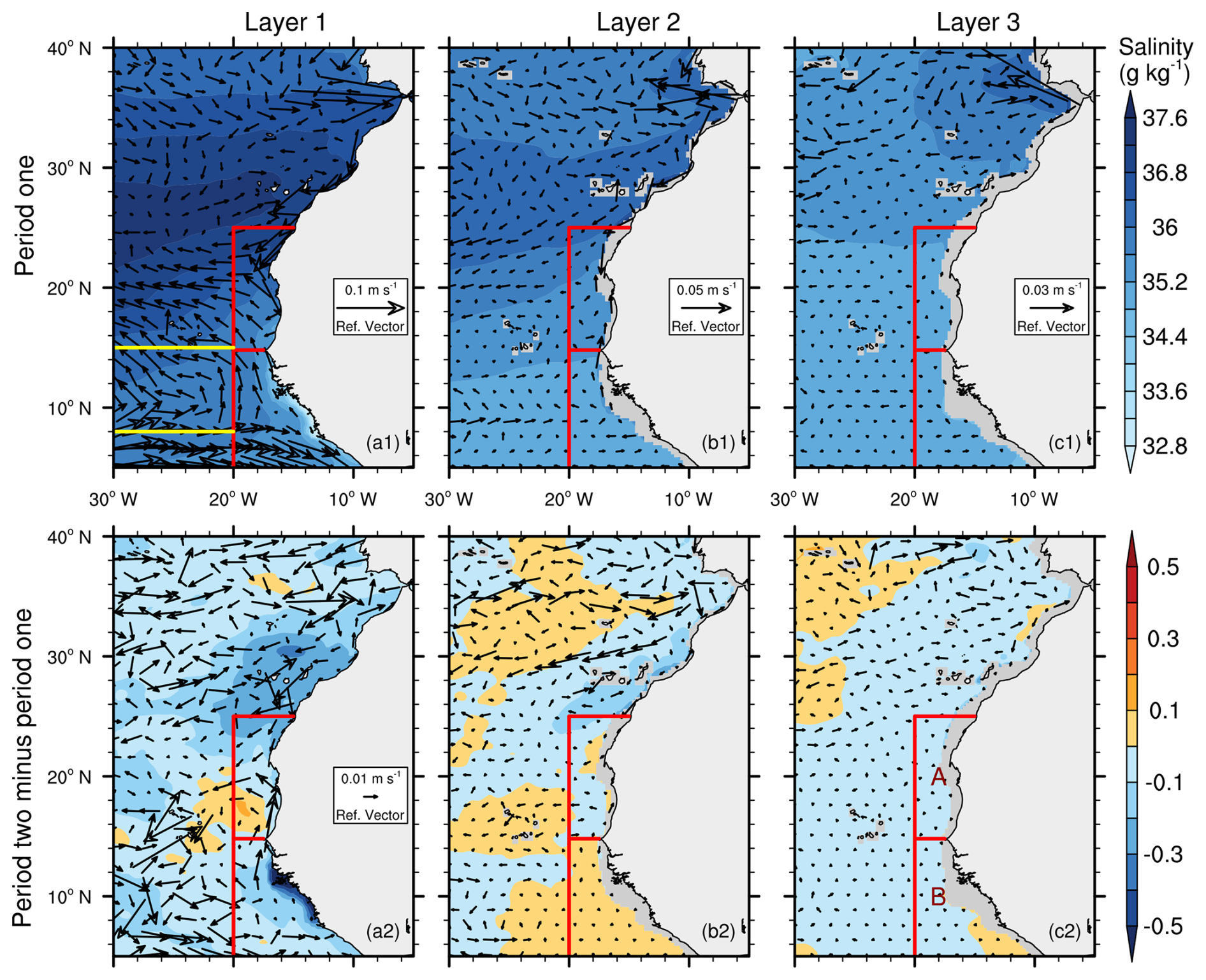
Figure 9 Salinity and ocean current structures and their multi-year changes. (a1, b1, c1) Multi-year (period one) mean salinity and vector currents in layers 1–3, respectively. (a2, b2, c2) The same as a1–c1 but for period two minus period one. Notice the Guinea Dome indicated by the cyclonic circulation region between 8–18° N in (a1). The red lines delineate the domain, subdoimain A, and subdomain B, and the yellow lines indicate the cyclonic circulation in the Guinea Dome region, between the North Equatorial Current and Countercurrent.

We therefore hypothesize that subdomain A freshening associated with the multidecadal strengthening of F_net has its origin in salinity changes occurring elsewhere in the North Atlantic. To show the plausibility of this hypothesis, in the next section, we summarize the established literature on the eastern North Atlantic currents that affect subdomain A, and isolate pathways to subdomain A where salinity variations have a large number of common causes with subdomain A salinity variations, i.e. pathways where salinity variations and subdomain A salinity variations have the largest correlation coefficient (Brunt, 1917).

4 Freshening of the Canary Current by North Atlantic water masses

The most prominent ocean current traversing subdomain A is the southward-flowing Canary Current, a relatively shallow (about 200–300 m deep) eastern boundary current of the North Atlantic Subtropical Gyre conveying North Atlantic Central Waters (Zenk et al., 1991; Mason et al., 2011; Pelegri and Peña-Izquierdo, 2015). The water feeding the Canary Current is mainly supplied by two currents that converge around 35° N: the first is the equatoward Portugal Current and Portugal Coastal Current system between 35–45° N and 10–20° W, and the second is the eastern branch of the so-called “Azores Current,” a relatively deep (down to about 2000 m) narrow zonal jet that originates in the North Atlantic area where the Gulf Stream bifurcates (Barton, 1998, 2001; Martins et al., 2002; Mason et al., 2005). The Azores Current propagates east-southeastward between 33–35° N towards the African coast and the Gibraltar Strait (Klein and Siedler, 1989; Stramma and Müller, 1989; Jia, 2000; Martins et al., 2002; Comas-Rodríguez et al., 2011; Mason et al., 2011; Frazão et al., 2022).

Figure 9a1, b1, and c1 shows the domain horizontal currents and salinity averaged in layer 1, 2, and 3, respectively, and Fig. 7a2 and b2 show the time series of mean monthly salinity anomaly averaged in these layers for subdomains A and B. The linkage between the Azores Current and the Canary Current is particularly evident in layer 2 (Fig. 9b1). Compared to period one, in period two the Canary Current strengthened by about 0.01 m s⁻¹ in northern subdomain A where salinity decreased by up to 0.4 g kg⁻¹ (Fig. 9b2).

Owing to the complex nature of advection and dispersion in the ocean that distort the propagation of salinity signals between two locations, it is difficult to ascertain the origin of the salinity variation that caused subdomain A freshening. Nonetheless, the aim here is to show that subdomain A freshening is likely because of fresher-water supply to the source region of the Canary current. To do this, we used the approach of Salomon et al. (1995); Brown et al. (2002) and compared salinity time series at every model grid point in the North Atlantic with subdomain A salinity time series at different time lags. This cross-correlation technique is far from conclusive because the time lags (i.e. transit times) derived from it are sensitive to dispersive processes in the ocean such as mixing, diffusion, entrapment in gyres etc. To partly overcome this, Brown et al. (2002) suggest smoothing the data to remove high-frequency fluctuations, which enhances the advective aspect of the propagation of the salinity signal, before calculating the cross-correlations. We adopted this approach and applied a 107-month (about 9 years) low pass filter (moving average) to the salinity time series. We chose this filter window size to minimize salinity fluctuations at time scales below the decadal time scale (i.e. to minimize year-of-the-decade effects).

We calculated the Spearman cross-correlation of salinity averaged in layers 2–4 at each model grid point in the North Atlantic with subdomain A salinity averaged in layer 2 and averaged in layer 3. We chose these layers because (i) short-term air-sea fluxes that modify salinity are mostly attenuated below layer 1 (50 m), (ii) layers 2 and 3 account for 71.6 % of the total steric expansion in subdomain A (not shown), and (iii) layers 2 and 3 have large halosteric shifts in subdomain A during period two compared to layer 1 and 4 (Fig. 7a2).

In both layer 2 and 3 there is a large correlation (≥0.6) between subdomain A salinity and salinity along the Azores Current pathway (Path 1) and along the Portugal current and Portugal coastal current system pathway (Path 2) (Fig. 10a1, and b1); Path 1 and Path 2 are evident in the spatial pattern of layer 2 average horizontal velocity averaged during 1985–2018 (Fig. 11a and they are indicated in Fig. 11b for clarity. This means that subdomain A salinity fluctuations in layers 2 and 3 and salinity fluctuations along Path 1 and along Path 2 have a large number of common causes. The correlation coefficient spatial pattern is similar for subdomain A salinity averaged in layer 2 and averaged in layer 3, but the correlation coefficient magnitudes are larger when subdomain A salinity is averaged in layer 3 (Fig. 10a1 and b1), suggesting a stronger association between salinity fluctuations in subdomain A layer 3 and salinity fluctuations in the North Atlantic below the 50 m depth.

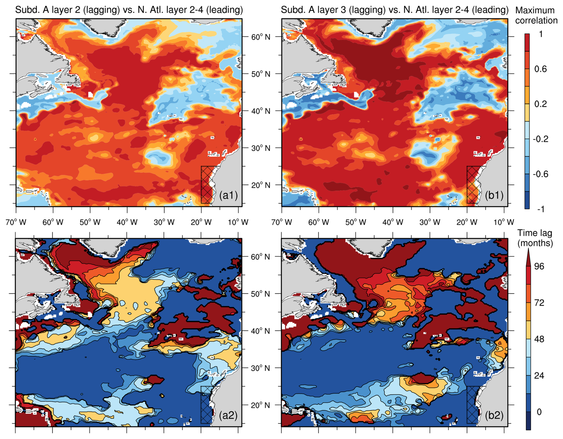
Figure 10 Physical linkage between subdomain A (subd. A, hatched region) salinity and salinity elsewhere in the North Atlantic. (a1) Maximum spearman cross-correlation between salinity averaged in subdomain A layer 2 (lagging) and salinity averaged in layers 2, 3, and 4 at every model grid point in the North Atlantic (leading) (a2) The time when the maximum correlation in (a1) is obtained. (b1) The same as (a1) but for salinity averaged in subdomain A layer 3. (b2) The time when the maximum correlation in (b1) is obtained. The dataset period is 1985–2018, but a 107-month low-pass (moving average) filter is applied to attenuate dispersion of salinity, that is, to minimize fluctuations at time scales below the decadal time scale. Thus the period for the cross-correlation calculations is July 1989–June 2014.

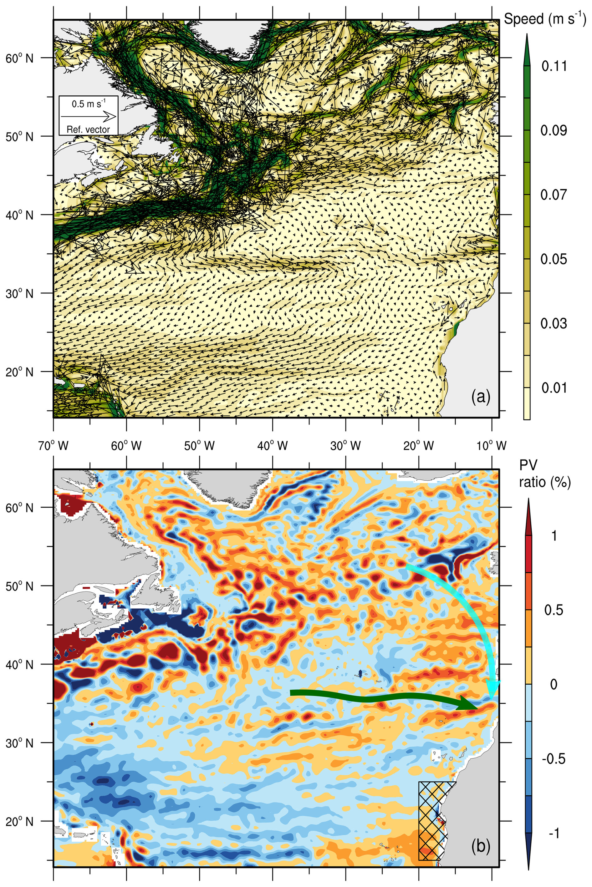
Figure 11 Physical relation between subdomain A salinity change and salinity changes elsewhere in the North Atlantic. (a) Time (1985–2018) and layer 2 average currents. (b) PV ratio (Eq. 6) calculated between the depths of density layer 1025 kg m⁻³ and density layer 1028 kg m⁻³, i.e. layers 2 and 3, see Eq. (5) and Fig. 6a2. The green colored curve indicates the Azores Current (Path 1) and the cyan colored curve indicates the Portugal Current and Portugal Coastal Current (Path 2).

Focusing on subdomain A and the region north of it up to about 40° N, the time lags (in which the maximum correlations are obtained) increases from south to north, suggesting that in this region the transit time for the salinity signal increase with distance from subdomain A (Fig. 10a2 and b2). For subdomain A salinity averaged in layer 2, the spatial pattern of the time lags appears to trace out Path 1 westward up to about 35° W (Figs. 10a2 and 11a and b: green curve).

On balance, notwithstanding the weakness of the cross-correlation technique, the presented evidence suggests that subdomain A salinity fluctuations at the decadal time scale is associated with salinity fluctuations in currents along Path 1 and 2 that supply the Canary Current flowing into subdomain A, which supports the hypothesis that subdomain A salinity variations has its origin in salinity changes occurring elsewhere in the North Atlantic. There is a research opportunity to classify the period of propagation of salinity signals in the North Atlantic.

These results highlight a possible multidecadal linkage between sea level anomalies in the eastern tropical margin of the North Atlantic and salinity anomalies in waters carried to this region by currents. Because the currents flowing along Path 1 and Path 2 also bring water to the source region of the Mediterranean inflow near the Strait of Gibraltar (Figs. 9a1, b1, and c1, and 10), there is a possibility of this same multidecadal linkage for the Mediterranean Sea. Indeed, analysis of numerical experiments by Jia (2000) and (Özgökmen et al., 2001) suggest that the emergence of the Azores Current is associated with the water sink generated in the eastern boundary by entrainment of the Mediterranean outflow (as it descends the continental slope) and by the Mediterranean inflow. Experimental research is needed to classify the modes of variability of currents along Path 1 and Path 2 and their linkages to ocean dynamics in the eastern boundary of the North Atlantic.

Holliday et al. (2020) reported that, owing to unusual winter wind patterns that rerouted Arctic-origin freshwater, in 2011 the largest freshening event in 120 years occurred in the subpolar North Atlantic area. To speculate on the possible origin of the fresher-water propagated to subdomain A, we calculated and analyzed the potential vorticity, a conservative flow tracer that characterizes ocean water mass, in the North Atlantic. Introducing f (s⁻¹) for the planetary vorticity, ζ (s⁻¹) for the relative vorticity, and H (m) for the difference between the depth of two density surfaces (1025 and 1028 kg m⁻³), the potential vorticity, PV, is given by Apel (1987)

$$\begin{array}{}\text{(5)}& {\displaystyle }{\displaystyle }\text{PV}={\displaystyle \frac{f+\mathit{\zeta }}{H}}.\end{array}$$

We chose these density surfaces based on the density boundaries between layers 1 and 2 and between layers 3 and 4 (Fig. 6a2), which means that we are tracing layers 2 and 3 waters. Conservation of potential vorticity implies that, away from boundaries and the sea-surface, the ratio of the quantities on the right-hand side of Eq. (5) is conserved following the motion of a water mass parcel. Thus, variations in PV show variations in the associated water mass. To compare period one PV (PV_period 1) and period two PV (PV_period 2) while preserving the PV pathway, we used a PV ratio metric given by

$$\begin{array}{}\text{(6)}& {\displaystyle }{\displaystyle }\text{PV}\text{ratio}=\left({\displaystyle \frac{{\text{PV}}_{\text{period 1}}}{{\text{PV}}_{\text{period 2}}}}-\mathrm{1}\right)\times \mathrm{100}.\end{array}$$

Equation (6) means that when PV_period 1 is greater than PV_period 2, PV ratio is positive: these are the light colored regions in Fig. 11b; and when PV_period 1 is less than PV_period 2, PV ratio is negative: these are the dark colored regions in Fig. 11b.

The spatial pattern of the PV ratio shows larger PV during period two along the axis of the Gulf Stream before it bifurcates (70–45° W, 35–50° N, Ikeda, 1993), along the northwest and northeast branches of the bifurcated Gulf Stream, in the regions of Path 1 and Path 2, and in subdomain A (Fig. 11b). Overall, there appears to be a connection between water mass variations in all these regions during period two. This may be related to the fact that several currents in the eastern North Atlantic are supplied by the North Atlantic Current (Krauss and Käse, 1984; Barton, 2001; Martins et al., 2002; Mason et al., 2005), which enables variations in the Gulf Stream to spread out. Cataloguing the timescales of interaction between eastern North Atlantic currents can be useful for anticipating fluctuations of seawater properties, especially in coastal areas.

5 Changes in horizontal and vertical velocity distributions and in water accumulation

The domain has a complex horizontal and vertical current system. Notwithstanding the limited scope of this study, we give a plausible explanation for the domain-wide water accumulation.

Mass gain (G in Eq. 3, Fig. 4b) contributed 18.4 % and 15.4 % of the multidecadal sea level increase in subdomains A and B (Table B1), respectively. The mass gain in subdomain B is entirely dominated by PminusE (20.1 %), whereas the mass gain in subdomain A is almost entirely because of ocean currents, F_net (17.3 %). It is interesting to note that the mean sea level is higher in subdomain B compared to subdomain A (Fig. 1b) and the multidecadal increase in sea level is larger in subdomain B compared to subdomain A (Fig. 4a). This would imply surface geostrophic flow to the east, but the solid coast blocks this flow causing it to travel parallel to the coastline, resulting in intensified alongshore currents from subdomain B to subdomain A.

Our hypothesis to explain this mass gain is that the mutual adjustment of horizontal and vertical current distributions in this margin is associated with water accumulation in the domain. The first evidence for this adjustment is the stronger upwelling in subdomain A during period two. In layer 1, there is an area of increase in salinity in the southern part of subdomain A, between 15–19° N (Fig. 9a2). However, the horizontal currents that flow into this area originate from regions with decrease in salinity (Fig. 9a2). This area of increase in salinity must therefore result from upwelling of cooler, higher-salinity waters from beneath. The temperature of the area decreased by up to 2 °C in period two (Fig. 12a3 and b3), and the PV ratio there is positive, implying changes in layers 2 and 3 water mass in this area (Fig. 11b).

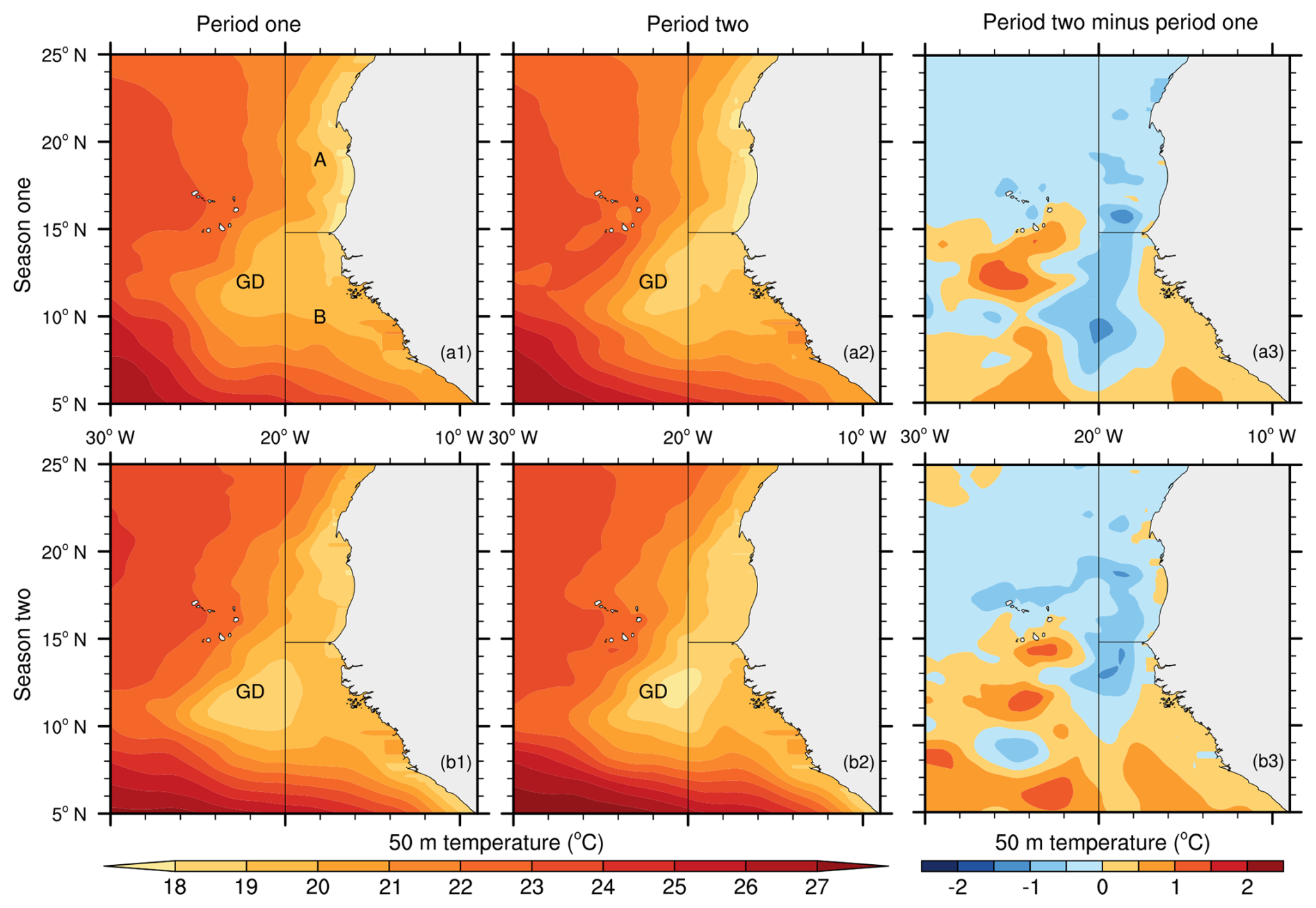
Figure 12 Thermal structure at 50 m depth, where the Guinea Dome (GD) is better developed (Mazeika, 1967; Doi et al., 2009) and its multi-year mean shift. (a1–a3) season one (March–October) mean potential temperature in period one, period two, and period two minus period one. (b1–b3) the same as a1–a3 but for season two (November–April). Notice the warming between 10–15° N.

The second evidence, which is likely related to the first, is the change in period two in the structure of the so-called “Guinea Dome,” a permanent, quasi-stationary feature adjacent to subdomain B between the westward-flowing North Equatorial Current and the eastward-flowing North Equatorial Countercurrent. This thermal dome is characterized by upward flux of cooler water from beneath that causes doming (upward displacement) of isotherms (Mazeika, 1967; Siedler et al., 1992; Yamagata and Iizuka, 1995; Doi et al., 2009, 2010). Layer 1 averaged horizontal currents show a cyclonic (anticlockwise) circulation region centered around 12° N and 22° W (Fig. 9a1). This is the core of the Guinea Dome (Fig. 12a2 and b2).

It is useful to first describe the connection between the water and thermal balance of the Dome before describing the Guinea Dome changes. From considerations of the continuity of water mass, in order for the displaced isotherms in the Guinea Dome to remain stationary, divergent (convergent) flow in the layer above the dome must be coupled to convergent (divergent) flow in a subsurface layer. Wyrtki (1964) offers an instructive illustration of the water balance of a thermal dome: consider a circular region of radius r (m) below the surface surrounding the dome core, the water flowing upward (downward) through this surface, with vertical average velocity w (m s⁻¹), must be removed (replaced) by horizontal water flow, with average velocity u (m s⁻¹), in a layer of thickness h (m) overlying the surface, thus

$$\begin{array}{}\text{(7)}& {\displaystyle }{\displaystyle }u\cdot \mathrm{2}\mathit{\pi }rh=w\cdot \mathit{\pi }{r}^{\mathrm{2}}.\end{array}$$

Equation (7) shows that a change in vertical velocity in the dome core is associated with a change in horizontal velocity in a layer above the dome. Because the displaced isotherms do not reach the sea-surface (Doi et al., 2009), which demonstrates that the dome circulation must be in thermal balance, the maximal w is thus limited by the heat energy available for warming the water from beneath as it ascends (Wyrtki, 1964). Accordingly, changes in the available heat energy implies changes in w, and consequently, changes in u in accordance with Eq. (7).

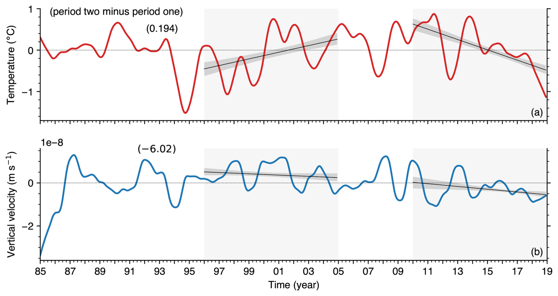
Figure 13 Monthly time series (mean annual cycle removed) of temperature and vertical velocity at 50 m depth in the Guinea Dome core (26–20° W, 10–15° N). (a) Potential temperature (temperature). (b) Vertical velocity, which is obtained as the negative of the horizontal velocity divergence at 50 m depth.

The changes in layer 1 horizontal velocity shows an anticyclonic (clockwise) circulation region north of the Guinea Dome center around 12–16° N and 22–26° W (Fig. 9a2). This circulation will weaken upwelling of cooler water from beneath. Furthermore, the circulation may cause a convergence zone, resulting in downwelling of warm surface water and heating below the surface. Indeed, an index of the dome thermal balance, the 50 m temperature in the dome core region (Mazeika, 1967), during different seasons shows that temperature below the surface in the anticyclonic circulation region increased by up to 1 °C during period two (Fig. 12a3 and b3), which give evidence for the downwelling of warm surface water. The time series of the 50 m temperature and vertical velocity, averaged in a box that covers the dome core (26–20° W, 10–15° N), show negative trends in period two (Fig. 13a and b), indicating changes in the Guinea Dome structure.

In summary, the evidence described above supports the hypothesis that the mutual adjustment of horizontal and vertical current distributions is associated with water accumulation in the domain. This hypothesis, moreover, suggests an interrelated pattern of multidecadal change in several permanent ocean elements operating in this region. Indeed, Cromewell (1958) suggested that the Costa Rica Dome in the eastern tropical Pacific Ocean, which exists in a similar topographic setting as the Guinea Dome (i.e. located in the northern edge of the North Equatorial Countercurrent and in close proximity to continental land-masses, in the eastern ocean boundary), is associated with cyclonic shear arising from the interaction of the countercurrent and a northward coastal current. There is a year-round northward coastal current off the northwest African coast (Ibrahim and Sun, 2022) and Fig. 9a2 shows a multidecadal shift in the horizontal currents in the northern edge of the countercurrent between 8–9° N lines of latitude. It is thus possible that the domain-wide water accumulation (Fig. 2b), the changes in the dome thermal structure and vertical velocity distribution (Fig. 13a and b), and the changes in horizontal velocity distribution (Fig. 9a2) are all varying on a multidecadal timescale.

One hypothesis that Wyrtki (1964) proposed for shifts in the Costa Rica Dome is that the cyclonic circulation separating the North Equatorial Current and Countercurrent (just as in Fig. 9a1) is unstable, probably because of fluctuations in the countercurrent strength and transport, which leads to recurring separation of eddies, and consequently, to shifts in the thermal dome structure. Further research is needed to obtain estimates of the timescale for which eddies separate from tropical thermal domes since it may be associated with sea level fluctuations in the tropical ocean margins. In situ under water observations, for example, can be useful for elucidating the annual variation pattern of thermal dome spatial structure in the ocean margins.

6 Conclusions

Reflecting on the results obtained from characterizing the evolution of sea level in the Atlantic margin off northwest Africa during a multi-year period of rising sea level (1996–2004) and pause in sea level rise (2010–2018), we arrive at the following conclusions.

• i.

  Of the various causes of sea level variation, the most effective during the 1996–2004 period of sea level rise are thermosteric and halosteric expansion, which contribute almost equally to domain-wide increase in sea level, with a small contribution from mass gain in the domain (Sect. 3.1).

• ii.

  The cause of the domain-wide pause in sea level rise during the 2010–2018 period is a large thermosteric contraction that counteracted halosteric expansion and mass gain (Sect. 3.1).

• iii.

  Relating to long-term sea level change, difference between means of 1996–2004 and 2010–2018, the most effective cause is domain-wide steric expansion, followed by vertical land movement and mass gain (Sect. 3.2). Thermosteric expansion is dominant in the southern subdomain, while halosteric expansion is dominant in the northern subdomain (Sect. 3.3). This halosteric expansion is associated with freshening of the Canary Current that traverses the northern subdomain (Sect. 4). There is evidence to suggest that the Canary Current source area was freshened by water originating elsewhere in the North Atlantic that reached the northwest African coast via two pathways: an open-ocean path that is consistent with the Azores Current, and a coastal ocean path that is consistent with the Portugal Current and Portugal Coastal Current system.

• iv.

  The results emphasize the role of salt as a key driver of long-term regional sea level change in this domain, a role that is not well recognized in the literature. This is especially important in the context of the globally changing climate because changes in local hydrological cycles can drive large changes in salinity, resulting in large changes in regional sea level.

• v.

  The results suggest a multidecadal linkage between sea level anomalies in the eastern tropical North Atlantic and salinity anomalies elsewhere in the North Atlantic. Thus, given satellite or in situ observations of salinity changes in the North Atlantic, it may be possible to anticipate coastal sea level changes in the northwest African coast.

• vi.

  The Canary Current source region is also the source region of the Mediterranean inflow near the Strait of Gibraltar (Sect. 4). It may therefore be possible also to anticipate multidecadal changes in the Mediterranean Sea characteristics based on observed changes elsewhere in the North Atlantic.

• vii.

  The mass gain contribution to the multidecadal sea level rise is dominated by ocean currents in the northern subdomain and by precipitation in the southern subdomain (Sect. 3). Domain-wide mass accumulation appears to be associated with the mutual adjustment of the vertical and horizontal velocity distributions inside the domain and in the Guinea Dome region on the west side of the domain (Sect. 5).

• viii.

  The dynamical adjustments of horizontal currents in the domain appear to be related to multi-year shifts in the characteristics of several permanent ocean elements operating in this tropical Atlantic region including the Guinea Dome thermal structure and vertical velocity, and horizontal currents in the northern edge of the North Equatorial Countercurrent (Sect. 5).

It is instructive to contrast the low-frequency thermal forcing and low-frequency remote haline forcing (that is realized through changes in the salinity of source water advected to the margin) of sea level in this ocean margin with the high-frequency local atmospheric forcing that is realized through changes in surface pressure over the margin. Considerations of the timescale and magnitude of sea level changes associated with these two forcing types facilitate design of sustainable infrastructure in coastal regions.

This work highlights an important need for a high-resolution atmosphere and coastal ocean two-way, coupled model to incorporate all current knowledge in this ocean margin, to provide a system for performing numerical experiments that will increase our understanding of the operating phenomena in this vitally important tropical region, and to facilitate better predictions. This type of 3D atmospheric and oceanic coupled model (Ibrahim et al., 2020), when nested with a larger domain ocean model and forced with land-surface hydrological inputs, can be used for experiments to identify and quantify critical processes that are involved in coastal open ocean exchanges. This will not only benefit neighboring countries through scientific management of coastal ocean resources, but it will improve our overall understanding of the North Atlantic basin dynamics and ocean-atmosphere interactions in ocean margins.

Appendix A: Summary of the causes of sea level displacement during period one and during period two

Table A1 Table of change in sea level displacement and its drivers during the rising state (period 1) and the hiatus state (period 2), see Sect. 3.1. Table values are obtained using Eq. (4) and the transport (F_net) is derived from Eq. (3).

Appendix B: Summary of the causes of multidecadal increase in sea level

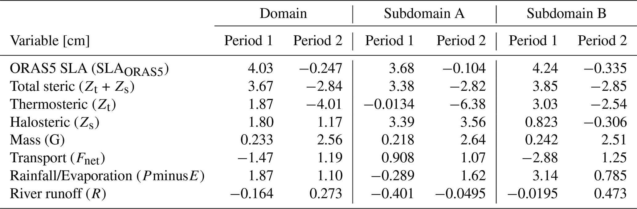
Table B1 Table values are the contribution of atmosphere and ocean variables to the relative increase in mean sea level between period one and period two: the values are period-2 mean minus period-1 mean (see Sect. 3.2). The values in parenthesis in column 2, 3, and 4 indicate the percentage contribution of each variable to the SLA rise (row 1) in the domain, subdomain A, and subdomain B, respectively. SLA=SLA_ORAS5 + barometric correction (ζ_a) + Boussinesq correction + vertical land motion (see discussion in method section). The total steric (residual Z_α) shifts reported in row two is obtained using the residual calculation approach (Eq.1).

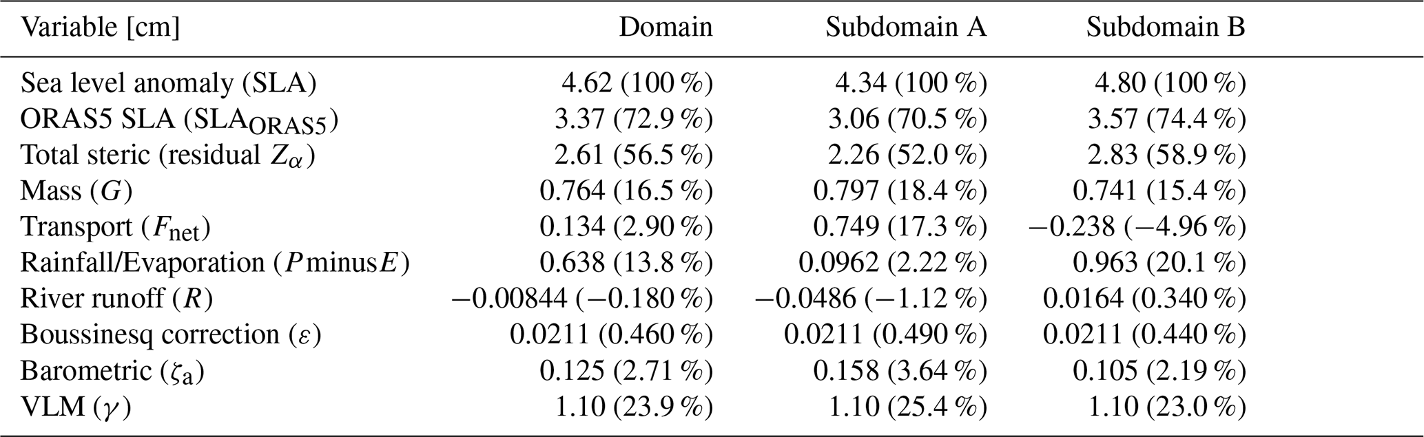
Table B2 Table values show the salinity-driven (halosteric) and temperature-driven (thermosteric) contributions to total steric shift obtained from direct calculations using Eq. (2). The values in parenthesis in column 2, 3, and 4 indicate the percentage contributions in the domain, subdomain A, and subdomain B, respectively.