Stratified-turbulence observations dominated by slantwise downward convective warm-water periods in the deep Mediterranean

A three-dimensional mooring array holding nearly 3000 high-resolution temperature sensors in 2500 m deep Mediterranean-Sea waters is used for a yearlong study on different sources of turbulent waterflows, which are vital for life. Although temperature differences are found never larger than 0.01 °C, daily, weekly, and seasonal variations are observed. With a delay of about a week, the deep-sea stratified turbulence tracks atmospheric disturbances, which are found 35 % more energetic in winter than in summer. About half the time, relatively warm stratified waters are moved to near the seafloor from 100's of meters higher levels. Combined internal-wave and sub-mesoscale eddy-induced motions lead to slantwise downward convective warm-water periods that are half an order of magnitude more turbulent than those induced via general geothermal heating from below, and about one order of magnitude more turbulent than those from open-ocean processes. The analysis estimates that eddy-induced stratified turbulence is likely more important for deep-sea life than rare, not observed, deep dense-water formation at the abyssal-plain mooring site.

1 Introduction

Irreversible, energy-consuming turbulence is indispensable for life everywhere on earth, including in the deep sea. Most ocean turbulence is generated near its boundaries, with an important input via the breaking of internal waves at steeply sloping underwater topography (Eriksen, 1982; Thorpe, 1987). Observational details of turbulence are still scarce from the abyssal deep sea that is commonly considered to be “quiescent and stagnant”. One of the key aspects in the breaking of internal waves is the “warming phase”, when, e.g., an internal wave moves downslope of topography and characteristically (re-)stratifies waters near the seafloor with near-homogeneous waters due to convection turbulence above (van Haren and Gostiaux, 2012). Restratification renders efficient turbulent mixing during the following upslope phase. Indirectly topography-connected are, perhaps less known, slantwise-moving, warm turbulent waters (van Haren and Dijkstra, 2021). This turbulence generation is possibly related with near-inertial waves and (sub-)mesoscale eddies in basins like the Mediterranean Sea where tides and stratified conditions are both weak. As will be demonstrated in this paper, these warm waters have the potential to generate larger turbulent mixing than in the open-ocean interior.

Under weakly stratified conditions, the potential of deep-sea turbulence generation via downward or slantwise moving waters should be compared with local general geothermal heating through the seafloor (e.g., Pasquale et al., 1996), and with deep dense-water formation from the surface (e.g., Marshall and Schott, 1999). Sparse shipborne microstructure profiling has provided estimates of turbulence contributions from different sources across the Northwestern Mediterranean in which geothermal heating is found more important than internal wave breaking (Ferron et al., 2017). However, details of relevant processes are lacking and require high-resolution moored observations over prolonged periods of time.

In a stably-stratified environment like the sun-heated ocean, downward motions of warm water reaching the deep seafloor seem impossible and counter-intuitive in relation with irreversible convection turbulence involving motion in three spatial dimensions “3D”. Natural, body-forced buoyancy-driven convection (e.g., Dalziel et al., 2008; Ng et al., 2016) applies to denser waters moving down and less dense waters moving up in narrow plumes, i.e. in terms of temperature variations: warmer waters moving up and cooler waters moving down. In the ocean, such buoyancy-driven convection turbulence occurs regularly in the upper O(10) m near the surface during nighttime (e.g., Brainerd and Gregg, 1995) and possibly lower 100 m above the seafloor (m a.s.f.) due to geothermal heating, depending on the local stratification. It can also occur as deep dense-water formation after specific preconditioning of stratification reduction near the surface in localized areas like polar seas and the Mediterranean during brief irregular, rare periods (Marshall and Schott, 1999). An exemption can occur when salinity dominates over temperature in contributing to density variations: if downward moving warm waters are sufficiently saltier than their environment, cooler and fresher waters may move up.

A reversible, also 3D, process occurs when internal-wave motions affect the stratified environment (e.g., LeBlond and Mysak, 1978). Such motions may displace relatively warm waters downward during a particular wave-phase, and cooler waters up. However, such displacements will not overturn and vertically mix the different water masses.

Nevertheless, an apparent counter-intuitive combination of irreversible and reversible processes was occasionally observed above a slope of Great Meteor Seamount where, in the weakly stratified waters underneath internal waves, convection turbulence was observed (van Haren, 2015). Whilst in those North-Atlantic Ocean waters the effects of salinity could not be excluded, confirmation was found in similar observations from fresh-water alpine Lake Garda (van Haren and Dijkstra, 2021). As these observations showed similarity with the warming phase of a nonlinear wave breaking above a sloping seafloor (e.g., van Haren and Gostiaux, 2012), it was suggested that the convection underneath internal waves was either generated via shear moving convection tubes slantwise, or via wave-accelerations overcoming vertical density differences in internal-forcing overcoming reduced gravity, instead of body-forcing overcoming gravity as in natural convection.

Similar to the effect of large-scale shear, planetary slantwise convection in the direction of the Earth's rotational vector may be brought about by the horizontal Coriolis parameter f_h (Marshall and Schott, 1999). The convection can be induced via resonantly-forced standing inertial waves under homogeneous conditions (McEwan, 1973). At mid-latitudes, apparently-stable stratification having buoyancy frequencies of N=f_h, 2f_h or 4f_h occur in marginal stability due to planetary slantwise convection (van Haren, 2008).

In this paper, the investigation is further pursued of slantwise downward convective warm-water periods inducing stratified-turbulence that occur frequently in the deep Western Mediterranean. For this purpose, a nearly half-cubic-hectometer large 3D mooring-array is constructed holding about 3000 high-resolution temperature T-sensors and deployed at a 2500 m deep seafloor. Turbulence calculations are made based on Ellison (1957) and Thorpe (1977) overturning scales for a full observational year to investigate potential seasonal variations therein. Governing physics processes that indirectly may affect deep-sea life by inducing or transporting sufficient turbulence for nutrient and oxygen supply are: atmospheric-disturbance generated near-inertial waves, boundary-flow instability generating sub-, O(1) km, and meso-, O(10–100) km, scale eddies. Motions associated with these processes dominate dispersal of water masses in seas and oceans. They are all greatly affected by the rotation of the Earth. They are however not considered to be part of irreversible “small-scale” turbulent mixing. How they transfer energy from the surface to deep-sea small-scales of turbulence dissipation is not yet fully established.

The materials and methods are described in Sect. 2, with an extension of turbulence calculation methods in Appendix A2. The results are presented in Sect. 3, which starts with a yearlong overview timeseries designating local variations in stratification conditions in comparison with the larger background stratification. The analysis then highlights periods under differently stratified conditions, before presenting yearlong timeseries of turbulence values, their improved statistics and short-scale variations. The various mechanistics and their effects on the deep sea are discussed in Sect. 4.

2 Materials and Methods

Sufficiently resolved temperature time series mainly from single mooring lines in well-stratified waters have proven useful for calculating turbulence values (van Haren and Gostiaux, 2012; Cimatoribus et al., 2014) using methods proposed by Ellison (1957) and Thorpe (1977). The original methods need some adaptation to be used in very weakly stratified waters like in the deep Mediterranean Sea. Turbulence values are calculated for dissipation rate of turbulent kinetic energy, henceforth “turbulent dissipation rate”, and, for a few instances, turbulent diffusivity.

2.1 Sampling network

In order to get some insight in the generation and development of deep-sea turbulence, 2925 independent, self-contained high-resolution NIOZ4 temperature “T”-sensors were distributed in nearly half-a-million cubic meters of seawater. Details of construction and deployment of the large-ring mooring can be found in van Haren et al. (2021). The large number of independent T-sensors is expected to improve statistics of turbulence values, in an environment where all dynamics is captured by temperature variations of less than 0.01 °C. The small temperature variations put a large strain on the technical capabilities of quantifying the deep-sea turbulence.

With two supplementary T-sensors registering tilt information above and below, 63 T-sensors were taped at 2 m intervals to 45 vertical lines 125 m tall that each were tensioned to 1.3 kN by a single buoy on top. The T-sensors were located between nominally h=1.5–125.5 ± 0.5 m a.s.f. and recorded data at a rate of once per 2 s. Three buoys, of lines 1.4, 3.5 and 5.7 (henceforth throughout the text, the original naming “group.line” is shortened without period; for layout see Appendix A1), held a single-point Nortek AquaDopp current meter at h=126 m, which recorded data once per 600 s. The lines were attached at 9.5 m horizontal intervals to a steel-cable grid that was tensioned inside a 70 m diameter steel-tube ring functioning as a 140 kN anchor.

The ensemble “large-ring mooring” was deployed on the <1° flat and 2458 m deep seafloor of 42°49.50^′ N, 006°11.78^′ E just 10 km south of the steep continental slope, 5 km from its abyssal-plain foot, of the Northwestern Mediterranean Sea, in October 2020 (Fig. 1a). At the site's (mid-)latitude f_h=1.08f. For calibration and reference purposes, a single shipborne Conductivity Temperature Depth “CTD” profile was obtained to h=0.5 m, about 1 km horizontally from the mooring site during the deployment cruise. Meteorological data were obtained from Island Station “Porquerolles”, 43°0^′ N, 006°12^′ E.

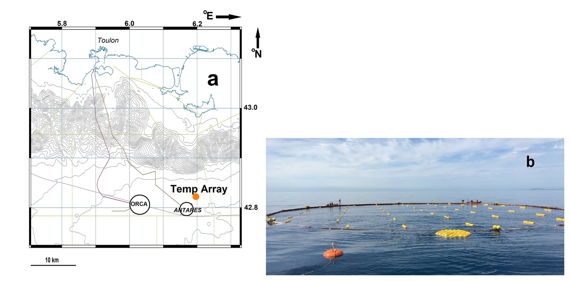
Figure 1 Large-ring mooring site and deployment. (a) Location named “Temp Array” (orange dot) on map off southern France. The mooring is well east of main neutrino-telescope site “ORCA” of KM3NeT (Adrián-Martinez et al., 2016) and just northeast of the former “ANTARES” neutrino-telescope site. Meteorological station is at Porquerolles Island, 20 km due North of Temp Array. Isobaths are drawn every 100 m. The grey lines indicate Toulon-harbour approach sectors. (b) At sea, during deployment finalizing the opening of air valves before sinking. The near part of the large steel-tube ring is already underwater. Almost all buoys of the 45 small-ring compacted vertical lines are visible (for layout see Appendix A1).

With the aid of Irish Marine Institute Remotely Operated Vehicle “Holland I” all 45 vertical lines with T-sensors were successfully recovered in March 2024. Of the lines, 43 were mechanically in good order. Line 18 was hit by the drag parachute, which functioned as a stabiliser during the free-fall deployment, whereby 10 sensors were lost. Line 65 was about 0.5 m lower than nominal because of a loop near the cable grid. Figure A1 in the Appendix shows the numbering of the lines, which were ordered in six groups for synchronisation purposes. As with previously deployed NIOZ4 T-sensors (for details see van Haren, 2018), the individual clocks were synchronised to a single standard clock every 4 h, so that all T-sensors were sampled within 0.02 s. Line 36 did not register synchronization, possibly due to an electric cable failure. Three T-sensors leaked and <10 were shifted in position due to a tape malfunctioning. After calibration, some 20 extra T-sensors are not further considered due to electronics (noise) problems. In total, 2882 out of 2925 T-sensors functioned as expected for the first 20 months after deployment, with remaining bias due to electronic drift resulting in deviations from absolute accuracy. Depending on the period and type of analysis considered, between 50 and 150 T-sensors showed too large bias requiring additional attention during post-processing of the records from the weakly stratified deep sea.

Due to unknown causes all T-sensors switched off unintentionally when the file size on the memory card reached 30 MB. This may have to do with a formatting or programming error. The dataset is 20 months long for sensors only registering temperature, and 3 months for those with tilt, though about 2.5–3 years is possible with the present setup.

2.2 Post-processing of temperature data

With respect to previous NIOZ4 T-sensor version, improvements of the electronics resulted in about noise levels of 0.00003 °C and a doubling in battery life. As described in van Haren (2018), calibration yielded a relative precision of <0.0005 °C, and <0.0001 °C after careful post-processing. Bias due to instrumental electronic drift of <0.001 °C month⁻¹ after aging was primarily corrected by referencing daily averaged vertical profiles, which must be stable from a perspective of turbulent overturning in a stratified environment, to a smooth polynomial without instabilities. In addition, because vertical temperature (density) gradients are so small in the deep Mediterranean, reference was made to periods of typically one hour duration that were homogeneous with temperature variations smaller than instrumental noise level (van Haren, 2022). Such periods were on days 350, 453, and 657 in the existing records. This secondary correction included low-pass noise filtering “lpf” of data with time. Under near-homogeneous conditions, a tertiary correction involved lpf of data in the vertical. Temperature records were pressure-corrected by transferring to Conservative Temperature Θ (IOC et al., 2010) using CTD's mean local salinity value. Henceforth, Θ will be named “temperature”, for short.

2.3 Turbulence values calculation for different stratification periods

Given the consistent and tight temperature-density relationship (Sect. 3), corrected temperature data allowed for calculations of turbulence values using the overturning displacement method of Thorpe (1977) by reordering density instabilities. Details for the method of calculating turbulence values from moored T-sensor data from well-stratified waters is given in van Haren and Gostiaux (2012). Here, the method is applied under weakly stratified conditions in which buoyancy frequency N≪10f, f denotes the local inertial frequency, the vertical Coriolis parameter. As the method by Thorpe (1977) is typically applied to profiling data, the vertical spacing of 2 m of moored T-sensors is sufficient to resolve Ozmidov (1965) and largest overturning scales, as has been verified in van Haren and Gostiaux (2012). The transition to the energetic turbulence regime occurs for scales >1.8 m under N=f using the buoyancy-Reynolds number threshold given in Gargett et al. (1984).

For the present deep-sea area, distinction is made between periods under environmental conditions when $N\sim >f$, somewhat exaggerating named stratified-water “SW” conditions, and $N\sim <f$ including unstable values, named near-homogeneous “NH” conditions. For NH, the tertiary correction is needed, and, when unstable overturns exceed the 124 m vertical range of sensors, an extra correction is mandatory because the Thorpe (1977) method of reordering is over-estimating displacements and resulting stratification (van Haren, 2025a). Such periods are difficult to trace, because of the extremely small vertical temperature differences, and the selection can only be done manually as it is inadequately automated.

For comparison with common Thorpe (1977) method, mean turbulence values are also computed using “Ellison”-scales (Ellison, 1957, for atmospheric data; Itsweire, 1984, for laboratory data; Moum, 1996, for oceanographic microstructure profiler data). Such scales are determined from moored T-sensor time series by filtering out internal wave and sub-mesoscale motions. The method is quite sensitive for the precise high-pass filter “hpf” cut-off frequency, as was noted for well-stratified Atlantic Ocean waters (Cimatoribus et al., 2014, for oceanographic moored T-sensor data). Appendix A2 proposes a modified version for application to moored T-sensor data under very weakly stratified conditions where filter cut-off frequencies are given for SW and NH conditions in the deep Mediterranean. For both methods, mean values are obtained from moored multiple-line T-sensor records after averaging over at least the largest turbulence scales, over the vertical “[…]”, over time “〈…〉”, and over 45 horizontally distributed lines “(…)”.

3 Results

3.1 General yearlong overview and large-scale stratification

The focus is on the first full year of observations to investigate potential seasonal variation in deep-sea turbulence dissipation rate values. The yearlong data-overview time series in Fig. 2 demonstrates 2–30 d variations, in waterflow speed (Fig. 2a), temperature (Fig. 2b), horizontal waterflow difference (Fig. 2c), and vertical temperature difference (Fig. 2d). Such time-variability is typical for sub-meso- and mesoscale motions, which are likely associated with the dynamically unstable, meandering boundary current over the canyon-incised steep continental slope (Crepon et al., 1982) and which may develop into eddies, with strongest flows near the surface and in winter (Albérola et al., 1995; van Haren and Millot, 2003).

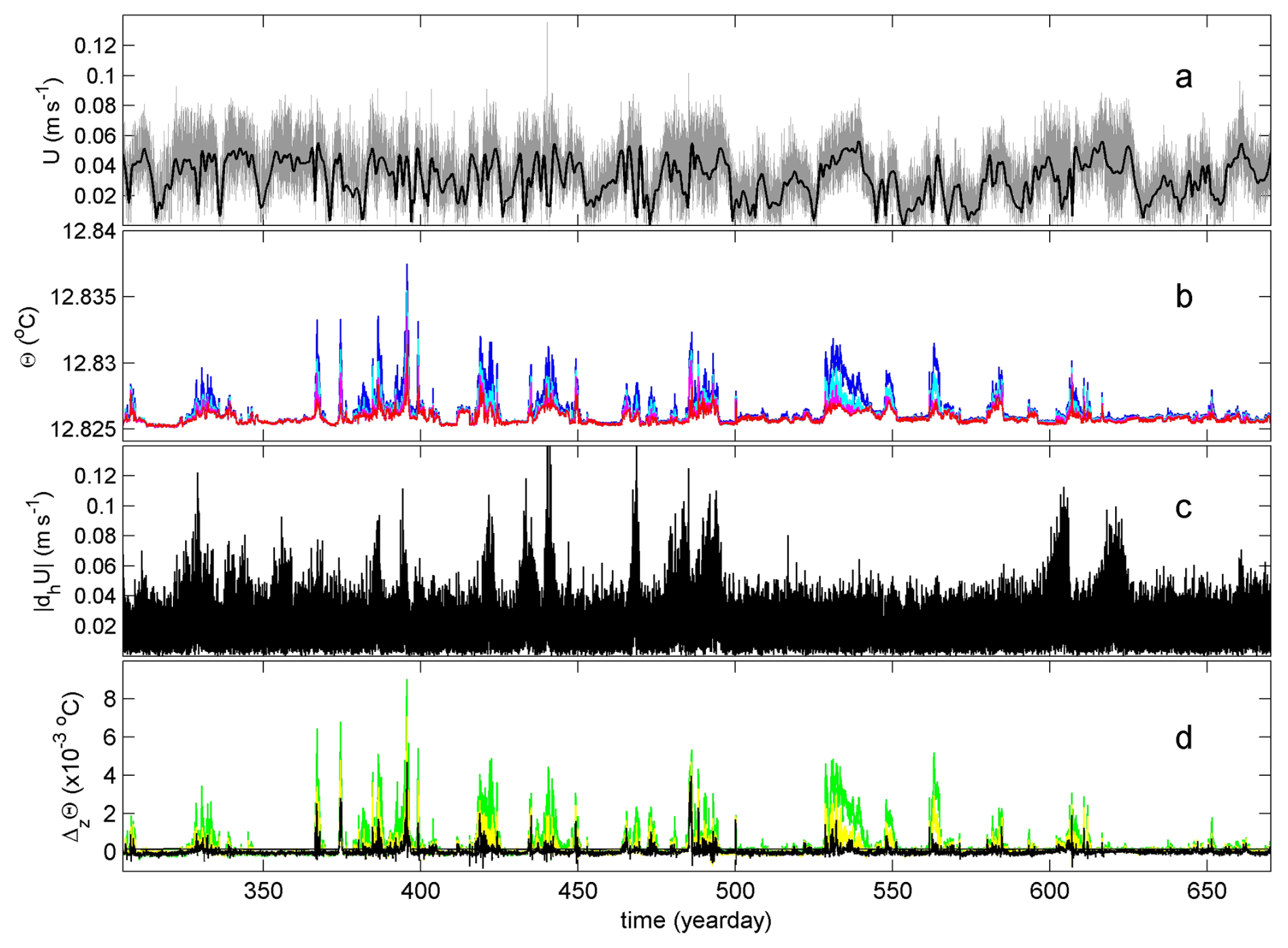
Figure 2 Time series of T-sensor and current meter data, for the first year of sampling data. Time in days of year 2020, +366 in 2021. (a) Unfiltered waterflow speed at h=126 m a.s.f. (grey) and daily filtered (black). (b) Conservative Temperature from vertical line 25, at h=1.5 (red), 29.5 (magenta), 59.5 (cyan) and 99.5 m (blue), corrected for drift and referenced to CTD-data of Fig. 3b. (c) Amplitude of horizontal waterflow differences. (d) Vertical temperature differences between the lowest T-sensor and those above from (b), between 99.5 and 1.5 (green), between 59.5 and 1.5 m (yellow), between 29.5 and 1.5 m (black).

Over the one year of observations, the deep-sea waterflow speed U seldom exceeds 0.1 m s⁻¹, with little variations through the seasons. U also rather strongly varies with local inertial period, which partially reflects the variable thickness of the graphical curves in Fig. 2a, and which may be understood from comparing the daily-filtered time series with the original one.

Inertial motions do not dominate T-sensor data (Fig. 2b and d). Also in contrast with U, the temperature data demonstrate a seasonal variation with relatively warmer (Fig. 2b) and more stratified (Fig. 2d) waters in winter, coarsely between days 365 and 495. This seasonal variation is also found in horizontal waterflow difference (Fig. 2c). The entire dynamical temperature variation over the year and up to h=125 m from the seafloor is captured within maximum $\left|\mathrm{\Delta }\mathrm{\Theta }\right|<\mathrm{0.01}$ °C, and commonly amounts only a few millidegrees.

About half the time, the temperature difference between h=1 and 125 m $\mathrm{\Delta }\mathrm{\Theta }>\mathrm{0.0002}\mathrm{°}\mathrm{C}\equiv T_{\text{thres}}$, a threshold level that is about six times the standard deviation of T-sensor noise level. This temperature difference provides an overall stratification resulting in N>0.65f. These relatively warm SW either come from above or from the side, slantwise downward. The other half of the time ΔΘ<T_thres, N<0.65f and stratification may be unstable, or NH conditions. Under NH, less than 0.7 % of total time negative temperature differences are found exceeding the (absolute value of) threshold level and corresponding with large-scale, >125 m developed geothermal heating. As a result, at the observational site convection turbulence associated with geothermal heating is suppressed by warm waters advected into the area most of the time.

Although the boundary current is strongest near the surface, it manifests itself at great depths including mesoscale variations at horizontal scales O(10–100) km. However, observed spatial waterflow variations over about 50 m horizontally also indicate much smaller-scale, rapidly-fluctuating differences (Fig. 2c). These variations associate, in absolute value, with warm SW conditions in approximately half the cases. No cooling, inversely stratified waters, from above are observed in the yearlong record.

Compared to open-ocean waters where large 100 m scale N>10f, the deep Mediterranean SW are characterized by weak stratification with N=O(f). Despite the relatively weak stratification, SW will prove important for turbulent mixing in the area.

The single shipborne CTD observations show no dominant influence of salinity over temperature governing density variations, in the lower 500 m a.s.f. (Fig. 3). Over the well-resolved stratified portion between $-\mathrm{2165}<z<-\mathrm{2055}$ m, the density-temperature relationship is found to be consistent (cf. van Haren, 2025a),

$$\begin{array}{}\text{(1)}& \mathit{\delta }{\mathit{\sigma }}_{\mathrm{2}}/\mathit{\delta }\mathrm{\Theta }=-\mathrm{0.25}\pm \mathrm{0.01}\mathrm{kg}{\mathrm{m}}^{-\mathrm{3}}\mathrm{°}{\mathrm{C}}^{-\mathrm{1}},\end{array}$$

where δσ₂ denotes the density anomaly referenced to a pressure level of 2×10⁷ Pa. Hence, Θ can be used as tracer for density variations to quantify turbulent overturning using the Thorpe (1977) reordering method.

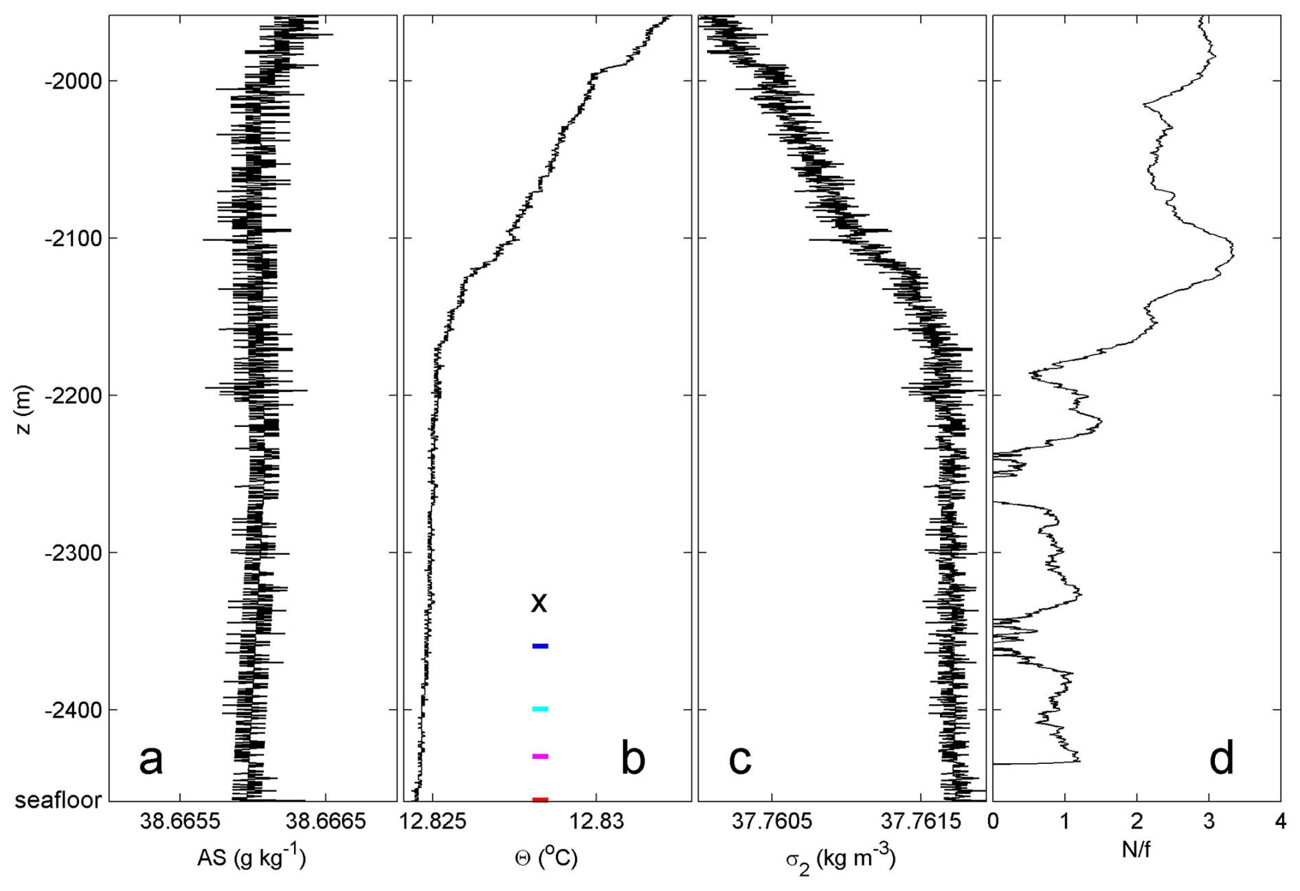
Figure 3 Lower 500 m of shipborne CTD profile obtained to within 0.5 m from the seafloor (at $z=-\mathrm{2458}$ m). (a) Absolute Salinity, with x axis range similar to that of (b) in terms of contribution to density variations. (b) Conservative Temperature. The colored ticks indicate the vertical positions of the four T-sensors of which data are displayed in Fig. 2b. The “×” indicates the position of the current meter. (c) Density anomaly referenced to 2×10⁷ N m⁻². (d) Ratio of 25 m scale buoyancy frequency “N” over local inertial frequency “f”.

In the weakly stratified waters over a vertical range of 100 m, density stratification varies, so that N<1f or NH is found near the seafloor, and N≈2f or SW around $z=-\mathrm{2050}$ m (Fig. 3d). Over 25 m vertical ranges, N≥2f can be found (Fig. 3d), and over 1–10 m ranges N>4f may be inferred from Fig. 3c around $z=-\mathrm{2110}$ and −1980 m. Such thin stratified layers are occasionally also found at greater depths if the better-resolved temperature profile is investigated (Fig. 3b). While the occasional vertical temperature differences of <0.01 °C in Fig. 2d could result from horizontal differences or fronts, it seems more likely that stratification of around $z=-\mathrm{2050}$ m in Fig. 3 is periodically lowered by action from above. Such action is expected down to about h<10 m from the seafloor, a thin layer in which vertical temperature differences are generally very small but not always (black graph in Fig. 2d).

Thus, although the moored T-sensors were located between the seafloor and $z=-\mathrm{2332}$ m, CTD-measured stratification may vary considerably with depth and time, and physical processes may lower warmer water some 400 m or advecting such waters slantwise, or possibly quasi-horizontally into the range of T-sensors. The precise direction of warm-water motion cannot be determined from single-station profiles, but may be resolved with a properly scaled 3D mooring-array. First however, details are investigated from different stratified periods using T-sensors data from a single line.

3.2 1D-details of a stratified-water period

Considering an average 5 mK-amplitude warm-water period (cf. Fig. 2b), a 1.3 d depth-time detail from around day 485 is presented from single line 15 (Fig. 4). While waters seem depressed from h>125 m, the warming occurs in variable periods of <1 h (Fig. 4a). During the second half of the warming, 0.001 °C additional heat is observed near the top. Relatively warm waters reach the seafloor twice within an inertial period of 0.73 d, around days 485.45 and 485.80. The warming ends with two cooler-water fronts and large overturning reaching the seafloor around day 486.2.

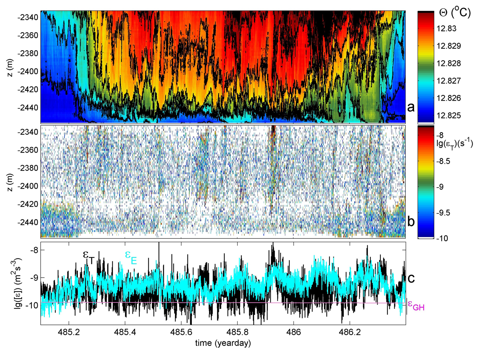
Figure 4 A 1.3 d period of relatively strong stratification with maximum small-scale buoyancy frequency N_max=6f, for data from vertical line 15. (a) Time-depth plot of Conservative Temperature with black contours every 0.001 °C. The horizontal axis is at the seafloor. (b) Logarithm of non-averaged turbulence dissipation rate from data in (a) using Thorpe (1977) method. (c) Time series of logarithm of data from (b) averaged over 124 m vertical extent of T-sensors (black), compared with calculations using Ellison (1957) method (cyan) with high-pass filter “hpf” cut-off from Fig. A2a.

The warming is depressed to within h<10 m from the seafloor, with a relatively large vertical temperature gradient between the cooler waters near the seafloor and the warmer waters higher up. This is reflected in the increased value of 2 m-small-scale buoyancy frequency N_s in h<30 m. Turbulent overturns hardly occur between days 485.2 and 486.15 for h<5 m, but are non-negligible in the stratified waters above for $\mathrm{5}<h<\mathrm{30}$ m, and are typically 50 m large for h>30 m (Fig. 4b).

Quantifying turbulence dissipation rate requires averaging, over all overturning scales possible, and 124 m vertically averaged values demonstrate variations with time over two orders of magnitude, when reordered data are used (Thorpe, 1977, method, black graph in Fig. 4c), or using $\mathrm{48}<\mathit{\omega }<\mathrm{3000}$ cpd (cycles per day) band-pass filtered data (Ellison (1957) method cf. Appendix A2, cyan graph in Fig. 4c).

Time-depth mean values for line 15 from SW's day 485 are: turbulence dissipation rate 〈[ε_T]〉=6 ± $\mathrm{3}\times {\mathrm{10}}^{-\mathrm{10}}$ m² s⁻³ and turbulent diffusivity 〈[K_z]〉=1.5 ± $\mathrm{0.7}\times {\mathrm{10}}^{-\mathrm{3}}$ m² s⁻¹ under buoyancy frequency 〈[N]〉=2.9 ± $\mathrm{0.3}\times {\mathrm{10}}^{-\mathrm{4}}{\mathrm{s}}^{-\mathrm{1}}\approx \mathrm{3}f$, using Thorpe (1977) method. Modified Ellison (1957)-method 〈[ε_E]〉=7 ± $\mathrm{3}\times {\mathrm{10}}^{-\mathrm{10}}$ m² s⁻³ (Appendix A2). There is some bias to low mean turbulence values by disregarding overturns below threshold, which is very low given the <0.0001 °C precision of T-sensors after post-processing (van Haren, 2018). However, this bias is well within the error of calculation as turbulence is dominated by the large energy-containing overturns. These mean turbulence values are more than one order of magnitude larger than open-ocean values observed in stratified waters well away from boundaries (e.g., Gregg, 1989; Polzin et al., 1997; Yasuda et al., 2021).

3.3 1D-details of a near-homogeneous period

For comparison, such turbulence values are under NH conditions between days 316.5 and 320.5 (Fig. 5): 〈[ε_T]〉=2 ± $\mathrm{1}\times {\mathrm{10}}^{-\mathrm{10}}$ m² s⁻³ and 〈[K_z]〉=1.1 ± $\mathrm{0.5}\times {\mathrm{10}}^{-\mathrm{2}}$ m² s⁻¹ under 〈[N]〉=0.5 ± $\mathrm{0.2}\times {\mathrm{10}}^{-\mathrm{4}}{\mathrm{s}}^{-\mathrm{1}}=\mathrm{0.5}f$. These values follow partially correcting the original method by Thorpe (1977) for overturns exceeding the height of instrumentation with information from manually selected NH environments that are bounded by stratification above (van Haren, 2025a). For periods with NH bounded by stratification above, such as between days 318.6 and 318.96, their mean turbulence dissipation rate is to within 10 % the same as found for periods with convection turbulence due to geothermal heating: ${\mathit{\epsilon }}_{\text{GH}}=\mathrm{1.2}\times {\mathrm{10}}^{-\mathrm{10}}$ m² s⁻³. The ε_GH matches average geophysical heat-flux observations in the area (Pasquale et al., 1996), under the condition that the mixing coefficient of Γ_C=0.5 (van Haren, 2025a), which is typical for buoyancy-driven convection turbulence (Dalziel et al., 2008). For this period, 〈[ε_E]〉=1.3 ± $\mathrm{1}\times {\mathrm{10}}^{-\mathrm{10}}$ m² s⁻³ (Appendix A2).

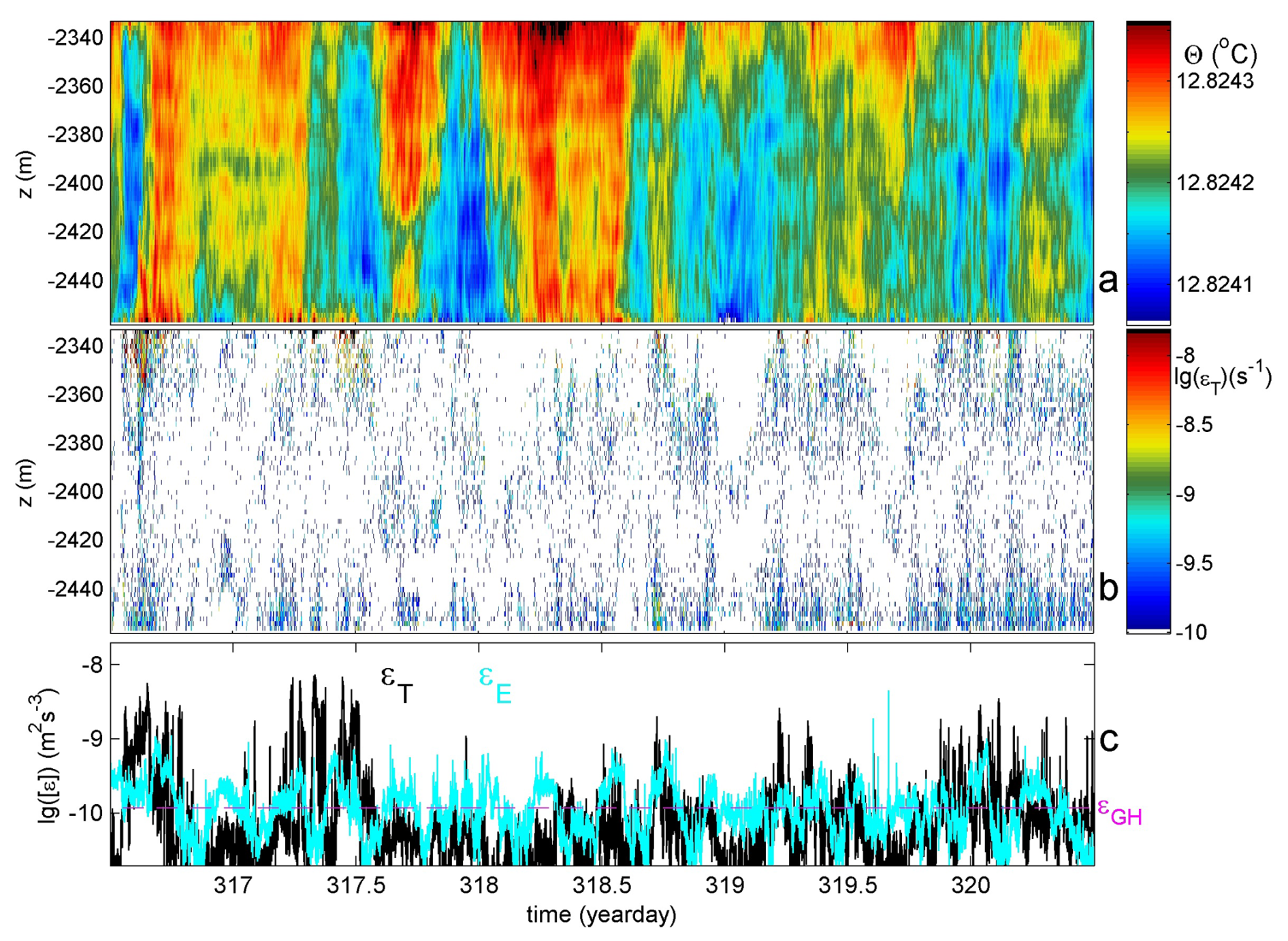
Figure 5 As Fig. 4, but for four days of near-homogeneous conditions with mean N≈0.5f, very weak stratification alternated with convectively unstable periods. For (c), the hpf cut-off for determining ε_E is shown in Fig. A2b and the magenta-dashed line indicates the average turbulence dissipation rate attributed to geothermal heating (see text).

3.4 Some 45-line statistics of short periods under SW and NH conditions

For consistency and statistics, six half-day periods are considered for computation of turbulence dissipation rate values, three under SW and three under NH conditions. The computations are performed for all 45 vertical lines and averages are computed over the 124 m height and half-day periods. It provides a one-and-a-half order of magnitude distribution of mean turbulence dissipation rate values (Fig. 6).

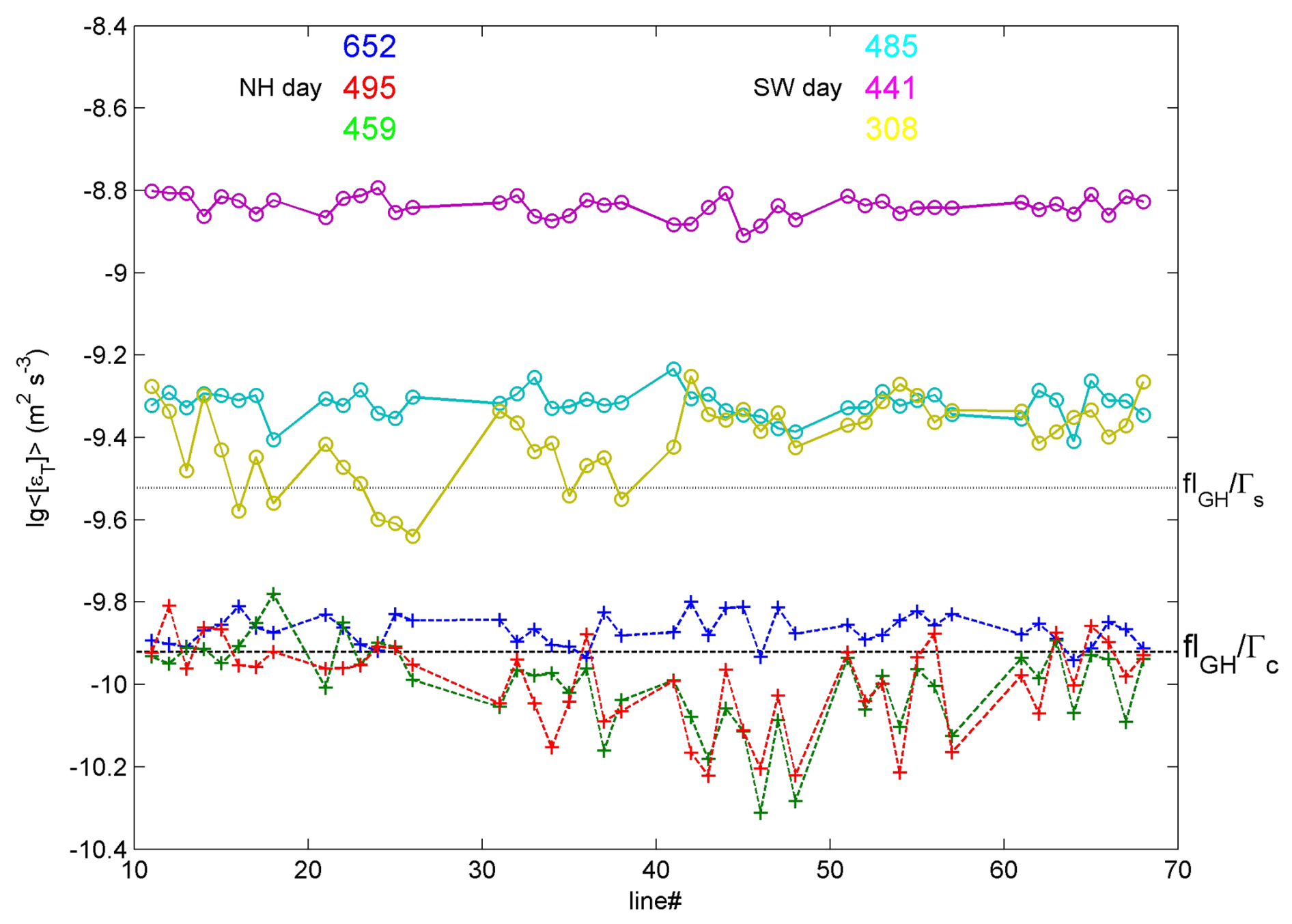
Figure 6 Limited statistics of Thorpe (1977) method (logarithm of) turbulence dissipation rates averaged over 124 m vertically given for six 12 h periods indicated by day-number, as a function of all 45 lines that are indicated by their number “line#”. Two thresholds are given as a function of general average buoyancy flux “fl_GH” from geothermal heating, divided by mixing coefficient for convection-turbulence Γ_c=0.5 (Dalziel et al., 2008) and for shear-turbulence Γ_S=0.2 (Osborn, 1980; Oakey, 1982). Solid lines (∘) indicate Stratified-Water “SW” conditions, dashed lines (+) indicate Near-Homogeneous “NH” conditions.

While some values are highly consistent between lines, e.g. the most energetic period on day 441, others show a half-order of magnitude distribution of values like on day 459. Initially, this calculation was set-up to help identify biased T-sensors and the appropriate polynomial correction. After applied tertiary correction, remaining wide distributions are attributed to more general turbulence variability.

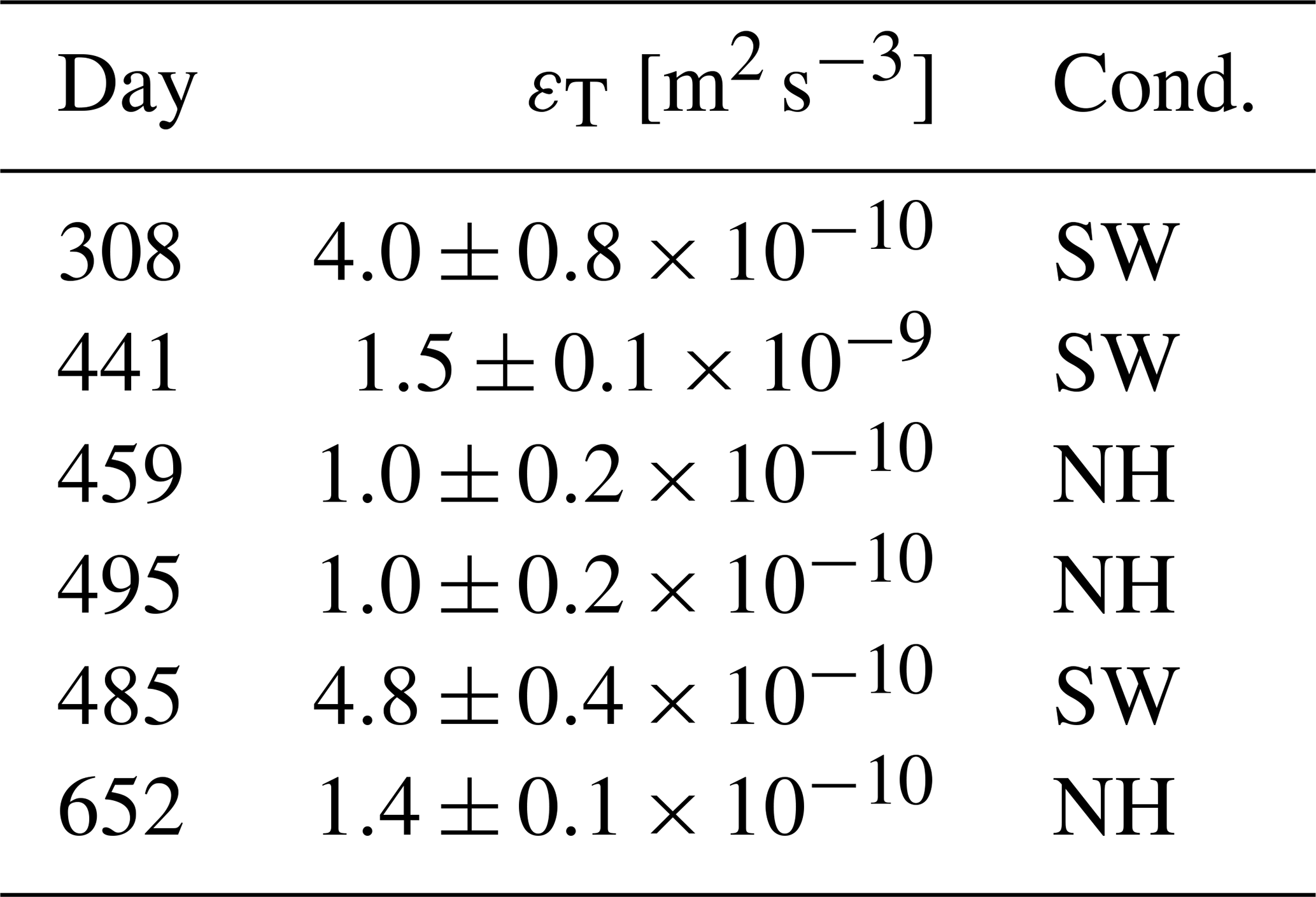
The statistics certainly improve turbulence dissipation rate values calculated using other instrumentation and methodology, which is generally to within a factor of two at best. The six examples of 45 lines provide about four times better statistics for the half-day periods (Table 1). The three NH values average to 〈[ε_T]〉_NH=1.1 ± $\mathrm{0.2}\times {\mathrm{10}}^{-\mathrm{10}}$ m² s⁻³, which is well within error equivalent to ε_GH as calculated from heat-flux measurements using mixing coefficient for convection-turbulence Γ_C=0.5 (Dalziel et al., 2008), while significantly different from the value for shear-turbulence Γ_S=0.2 typical for stratified conditions (Osborn, 1980; Oakey, 1982). It thus confirms previous results (van Haren, 2025a) and laboratory findings for convection-turbulence (e.g., Dalziel et al., 2008). The three SW values average to 〈[ε_T]〉_SW=8 ± $\mathrm{5}\times {\mathrm{10}}^{-\mathrm{10}}$ m² s⁻³, noting that the standard deviations of individual mean values are one order of magnitude smaller (Table 1).

Table 1 General first and second moment statistics calculated for 45-line, 124 m height, and half-day period turbulence dissipation rate values of Fig. 6. Two environmental conditions are characterized: SW = stratified-water, NH = near-homogenous, and may include geothermal heating. The two conditions are separated by a criterion equivalent of N=0.65f.

Another consequence of the use of multiple mooring lines besides improved statistics, is some insight in possible distribution of mean turbulence values. While one would expect erratic distribution over the short horizontal distances <70 m, particularly NH distributions yield two-dimensional consistent images such as on days 459 and 495 (Fig. 7). It provides confidence in consistency of methods used, but results in a puzzling gradient in turbulence that apparently is independent of waterflow (measured at h=126 m). For these geothermal heating- and near-inertial eddies-dominated periods the 9.5 m interval between lines seems reasonably well chosen, where 100 m may have been too large.

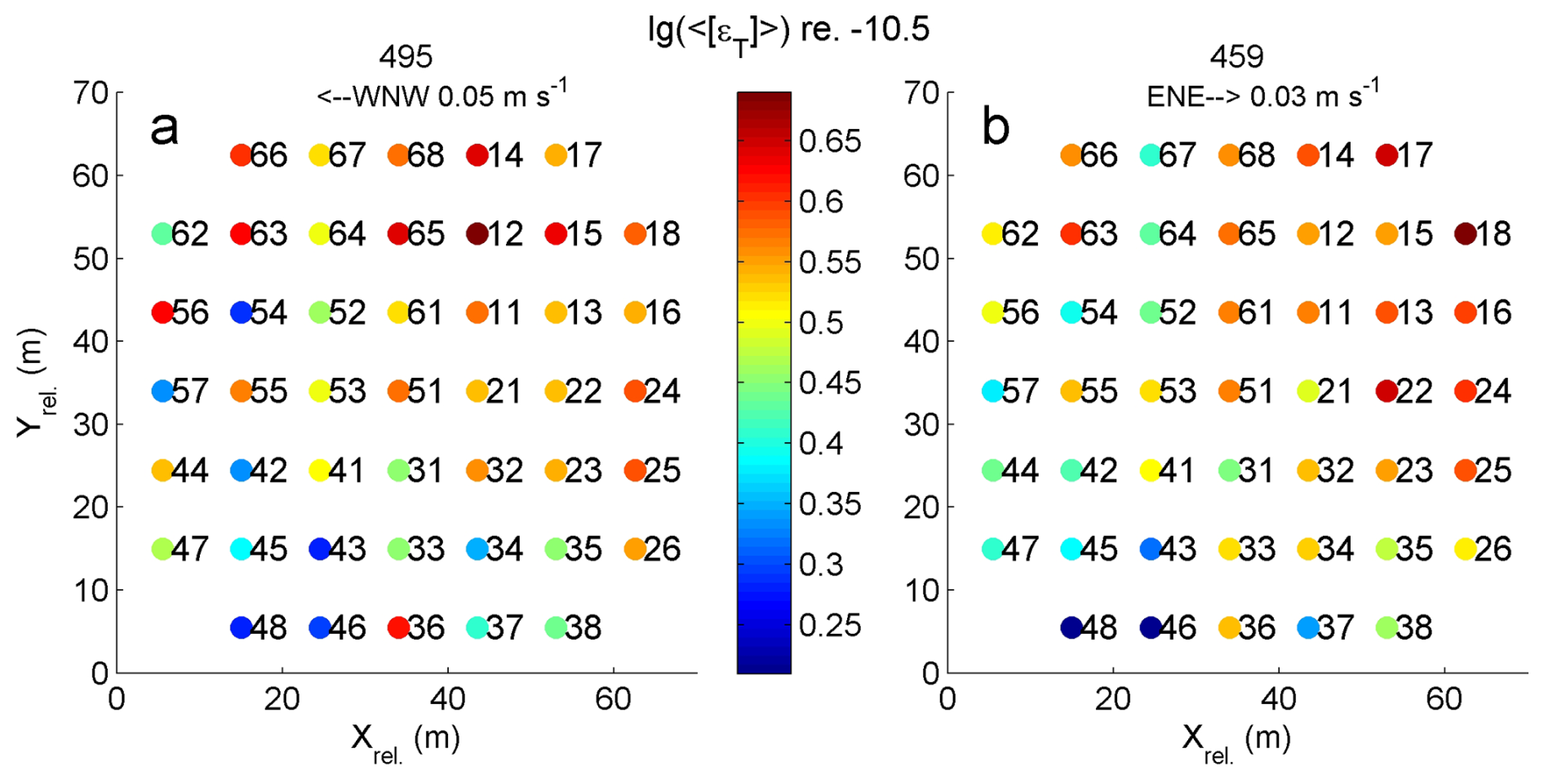
Figure 7 Plan view of 45 lines indicating logarithm relative to a value of −10.5 of time- and vertical-mean turbulence dissipation rates under NH conditions on days 495 (a) and 459 (b) of Fig. 6. On top, half-day mean waterflows are indicated.

3.5 Yearlong daily averaged turbulence dissipation rate values for 45 lines

A yearlong time series of daily-averaged turbulence values is computed for all 45 lines (Fig. 8). This computation is automated, using a fixed 3rd-order polynomial for primary correction. Since the tertiary correction for >125 m extending overturns is not applied manually, a criterion for excluding such episodes is used. This criterion is simply based on the daily-averaged temperature difference between uppermost and lowest T-sensor, per line. When ΔΘ<T_thres, given previously, the daily and vertical mean turbulence dissipation rate is fixed to,

$$\begin{array}{}\text{(2)}& \langle \left[{\mathit{\epsilon }}_{\mathrm{T}}\right]\rangle ={\mathit{\epsilon }}_{\text{GH}}=\mathrm{1.2}\times {\mathrm{10}}^{-\mathrm{10}}{\mathrm{m}}^{\mathrm{2}}{\mathrm{s}}^{-\mathrm{3}},\end{array}$$

the mean value for geothermal heating (van Haren, 2025a). This is found to occur 59 % ± 1.5 % of the time, somewhat varying per line, and characterizes NH, besides geothermal heating. About 40 % ± 1.5 % of the time is characterized by SW.

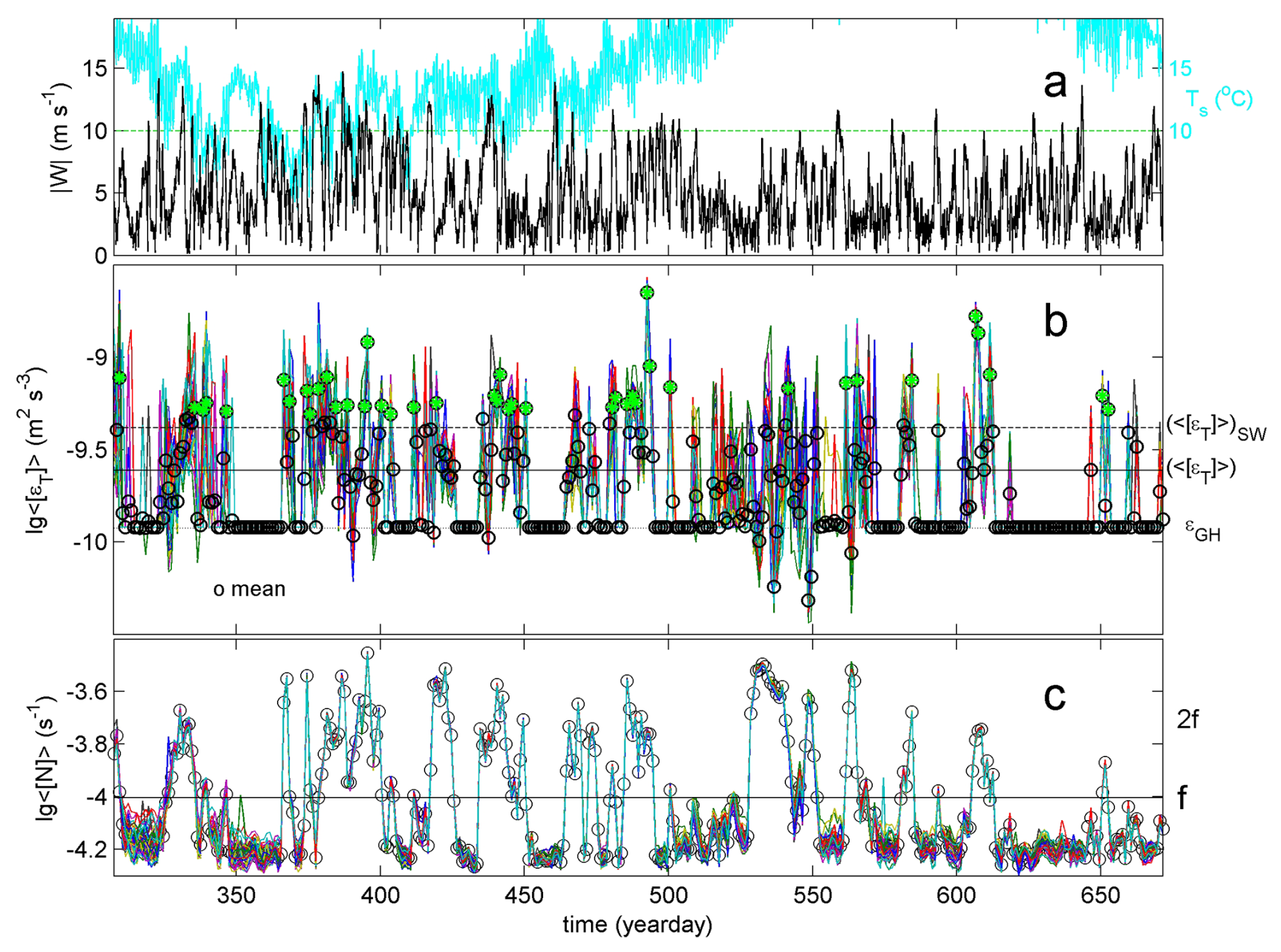
Figure 8 Yearlong time series of 45-line, daily, and vertically averaged turbulence dissipation rate and stratification values compared with meteorological data. (a) Wind speed (black) and surface temperature (cyan; scale to the right) measured at the station of Porquerolles Island, 20 km north of the mooring-array. The horizontal line is an arbitrary reference line below which near-surface ocean convection may occur under sufficient pre-conditioning. (b) Logarithm of daily and 124 m vertically averaged Thorpe (1977) method turbulence dissipation rate for all 45 lines (colour), including their mean values (black, circles) of which those exceeding twice the overall mean value (green asterisks). A threshold of 0.0002 °C is applied for $\mathrm{\Theta }(h=\mathrm{125}\mathrm{m})-\mathrm{\Theta }(h=\mathrm{1}\mathrm{m})$, below which values are forced to mean ${\mathit{\epsilon }}_{\text{GH}}=\mathrm{1.2}\times {\mathrm{10}}^{-\mathrm{10}}$ m² s⁻³, see text. The solid horizontal line indicates the overall mean value (Eq. 3), the dashed line the mean (Eq. 4) for periods under SW conditions. (c) Logarithm of corresponding mean buoyancy frequencies from reordered temperature profiles. The horizontal line indicates the local planetary inertial frequency.

The overall, yearlong, 125 m vertical, and 45-line mean turbulence dissipation rate amounts,

$$\begin{array}{}\text{(3)}& (\langle [{\mathit{\epsilon }}_{\mathrm{T}}]\rangle )=\mathrm{2.4}\pm \mathrm{0.2}\times {\mathrm{10}}^{-\mathrm{10}}{\mathrm{m}}^{\mathrm{2}}{\mathrm{s}}^{-\mathrm{3}},\end{array}$$

so that the mean SW turbulence dissipation rate amounts,

$$\begin{array}{}\text{(4)}& (\langle [{\mathit{\epsilon }}_{\mathrm{T}}]\rangle {)}_{\text{SW}}=\mathrm{4.3}\pm \mathrm{0.4}\times {\mathrm{10}}^{-\mathrm{10}}{\mathrm{m}}^{\mathrm{2}}{\mathrm{s}}^{-\mathrm{3}},\end{array}$$

which is thus closely represented by the short periods of days 308 and 485 in Fig. 6, Table 1.

Part of the SW-turbulence is attributable to geothermal heating in a layer of typically h=30 m under stratified waters. This may be inferred from the vertical temperature difference in that layer that passes T_thres during only 8 % of daily periods, cf. the magenta graph in Fig. 2d. Nevertheless, the advection of warmer waters suppresses geothermal heating-turbulence, possibly affecting the small-scale distribution in Fig. 7. The associated 3.5-times larger turbulence dissipation rates (Eq. 4) compared with geothermal-heating value (Eq. 2) are mainly generated by convection in conjunction with shear following internal-wave breaking.

Considering the yearlong “seasonal” variation that was suggested from the temperature (difference) time series in Fig. 2, and which is represented by the logarithm of daily and vertically averaged 〈[N]〉 in Fig. 8c, the corresponding plot of 〈[ε_T]〉 (Fig. 8b) is more difficult to interpret, also in conjunction with meteorological data (Fig. 8a). Different-line data mostly collapse on each other during winter between days 365 and 495, for both 〈[N]〉 and 〈[ε_T]〉. During this period, vertical-line daily mean turbulence dissipation rates most, 27 out of 41, exceed twice the mean value (Eq. 3), shown by the green asterisks in Fig. 8a. The 11 % of time of green-asterisks occurrence average to a mean turbulence dissipation rate of $\mathrm{7}\times {\mathrm{10}}^{-\mathrm{10}}$ m² s⁻³.

The average turbulence dissipation rate for the 130 d winter period is 25 % higher than the yearlong mean (Eq. 3). During this period, the wind work ∼W² is increased by 20 % compared to its yearlong average value. A rough visual correspondence is found between $\left|W\right|$ (Fig. 8a) and lg 〈[ε_T]〉 (Fig. 8b), the former leading the latter by about one week. The clearest value-collapse of turbulence and stratification data from different lines is found between days 450 and 500. The early-spring period is unlikely governed by deep dense-water formation due to limited meteorological forcing (Fig. 8a), but the preceding winter cooling may induce enhanced sub-mesoscale activity. Although increased sub-mesoscale motions can obscure near-inertial internal waves (van Haren and Millot, 2003), the transfer of energy to internal-wave scales leading to breaking and turbulence is not hampered. Possibly, as near-inertial shear is dominant in well-stratified waters, a shift from shear to convection turbulence may be associated with the increase of sub-mesoscale activity. Such potential energy transfer will be elaborated elsewhere.

In contrast, 14 % lower mean turbulence dissipation rate than Eq. (3) is found during the summer between days 540–670. In this period, W² is decreased by 13 % compared to its yearlong average value.

4 Discussion and conclusions

The observations show short O(10) day periods of typically 0.005 °C warmer waters than their environment appearing from above, but also, as inferred from the 3D mooring-array (movies in van Haren et al., 2026), from the sides, slantwise downward. The periods demonstrate a coarse near-inertial periodicity, which is much less deterministic than a tide, and twice the inertial periodicity. Like internal waves in the North-Atlantic Ocean and Lake Garda (van Haren, 2015; van Haren and Dijkstra, 2021), they push stratification to within a few meters from the seafloor. The pushdown is vigorously turbulent, more than one order of magnitude larger than in the open ocean away from boundaries. This relatively large turbulence should not surprise as both the bulk Reynolds number O(10⁶) and buoyancy Reynolds number ${\mathit{Re}}_{\mathrm{b}}=\mathit{\epsilon }/\left(\mathit{\nu }{N}^{\mathrm{2}}\right)=O\left({\mathrm{10}}^{\mathrm{4}}\right)>\mathrm{200}$ are large, thereby classifying it as energetic regime (Gargett et al., 1984), even in the weakly stratified deep sea. The $\mathit{\nu }\approx {\mathrm{10}}^{-\mathrm{6}}$ m² s⁻¹ denotes the kinematic viscosity. As geothermal heating is found to be relatively weaker from below, the convection turbulence seems to be driven by the, slanted, internal waves from above.

This slantwise convection turbulence is likely driven via (sub-)mesoscale eddies that are reinforced by atmospheric disturbances (Fig. 9). As such they may be compared with deep dense-water formation from sea-surface to seafloor that may occur over brief periods during a severe winter.

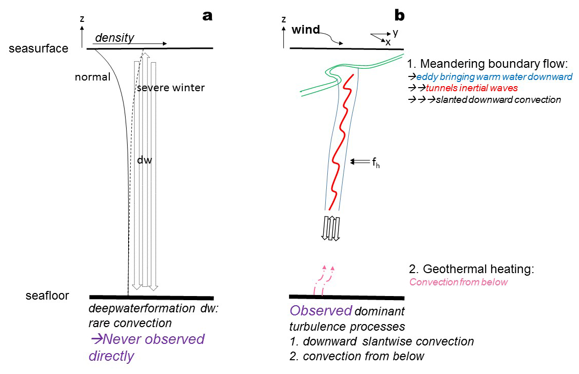
Figure 9 Sketch of potentially relevant flows and turbulence processes in the large-ring mooring area. (a) Rarely occurring, possibly once every 8 years during a severe winter but never directly observed (Thorpe, 2005), convection-turbulence due to deep dense-water formation when the vertical density profile changes from stable (solid graph) to unstable (dashed graph) over the entire 2500 m depth. (b) Wind-induced boundary flow meandering leading to alternating observations of deep-sea turbulence, from above, via dominant slantwise downward convection, and from below, via geothermal heating. The horizontal Coriolis parameter is indicated by f_h.

4.1 Warm-water convection versus hypothetic deep-water formation

While vertical motions by wintertime deep dense-water formation have been observed via moored observations, also in the Mediterranean (e.g., Schott et al., 1996), and floats (Steffen and D'Asaro, 2002), and surface buoyancy fluxes have been estimated to be O(10⁻⁷) m² s⁻³ during convection events (Marshall and Schott, 1999), quantification via observations of turbulence values associated with dense-water formation reaching the abyssal seafloor have yet to be made (Thorpe, 2005). Unfortunately, a dense-water event never reached the large-ring mooring while it was underwater. Estimates of deep-convection duration are limited, albeit that some consensus exists about decadal variability or occurrence of seafloor-reaching dense-water formation over a relatively short period of (less than) a week (Lilly et al., 1999), maximum a month, per 8–10 years (Dickson et al., 1996; Mertens and Schott, 1998). It is tempting to compare coarse deep dense-water formation turbulence dissipation rate estimates with those calculated from observations at the present mooring site during dominant warm-water convection under SW and geothermal heating under NH.

Because of the lack of measurements to quantify deep dense-water formation turbulence, some insight is gained from historic nocturnal convection-turbulence near the ocean surface. Microstructure measurements by, e.g., Brainerd and Gregg (1995) demonstrated turbulence dissipation rate values $>{\mathrm{10}}^{-\mathrm{7}}$ m² s⁻³ close to the surface and which decreased in the O(10) m near-homogeneous layer to typically,

$$\begin{array}{}\text{(5)}& {\mathit{\epsilon }}_{\text{DWF}}\approx {\mathrm{10}}^{-\mathrm{8}}{\mathrm{m}}^{\mathrm{2}}{\mathrm{s}}^{-\mathrm{3}},\end{array}$$

at a depth just above well-stratified waters below. The one order of magnitude reduced value reflects the erosion of the stratification. Here, we take value Eq. (5) as a proxy for turbulence dissipation rate by an event of deep dense-water formation-convection in waters just above the deep seafloor.

In comparison with geothermal heating's value (Eq. 2), Eq. (5) is two orders of magnitude larger. Where geothermal heating is quasi-permanent, deep dense-water formation rarely occurs, for example not at all during the presented 20 months of observations. Two orders of magnitude difference implies occurrence of Eq. (5) during one month per 8 years to match (Eq. 2). This is the estimated maximum at a given site.

In comparison with atmospheric-enforced mainly sub-mesoscale and internal-wave induced year-average value (Eq. 3), Eq. (5) would have to occur during 2.5 months per 8 years, or during 9 d every year. This is not observed in the open Liguro-Provençal basin. It implies that, either deep dense-water formation turbulence is stronger than Eq. (5) also for $z<-\mathrm{2000}$ m, which seems unlikely, or geothermal heating turbulence and especially SW turbulence are several times, SW turbulence up to one order of magnitude, larger than deep dense-water formation turbulence, when averaged over a decade in time. With their sources of sub-mesoscale eddies and near-inertial waves, the warm SW conditions thus seem more important than deep dense-water formation for supply of fresh materials in the deep-sea area. Recall that the observations are made in an area where tides, normally about half the ocean's mechanical energy source, are weak.

4.2 A comparison between turbulence from warm-water convection and geothermal heating

The observed yearlong mean turbulence dissipation rate value of SW being 2.5 times that of geothermal heating in the present area is the reverse of findings by Ferron et al. (2017), who find three times larger geothermal heating than SW from sparse microstructure profiling across the entire Northwest Mediterranean. The discrepancy may have to do with the location of the large-ring mooring, about 5 km from the foot of the continental slope and most likely regularly located under an eddy or meander of the well-stratified boundary current. These large-scale motions are intensified closer to the sea-surface (Albérola et al., 1995; van Haren and Millot, 2003).

Estimating turbulence dissipation rates from the microstructure profiler plots in Ferron et al. (2017) gives average values for h=100–600 m (the instruments were stopped some 90 m a.s.f.) of about $\mathrm{2.5}\times {\mathrm{10}}^{-\mathrm{10}}$ and $\mathrm{7}\times {\mathrm{10}}^{-\mathrm{10}}$ m² s⁻³, for the Western Mediterranean and specifically Ligurian Sea, respectively. These values are in the same range as mean and SW values (Eqs. 3 and 4), respectively. Both averaged microstructure profiles showed reduction in values in the lower h=100–200 m to about $\mathrm{1}\times {\mathrm{10}}^{-\mathrm{10}}$ and $\mathrm{3}\times {\mathrm{10}}^{-\mathrm{10}}$ m² s⁻³, respectively. For properly processed microstructure profiler data the instrumental error is to within a factor of two for mean turbulence dissipation rate values, not considering environmental variations. The shown values, from the same height above seafloor as the upper range of the moored T-sensors, compare with the geothermal heating- (Eq. 2) and mean- (Eq. 3) values determined at the large-ring mooring.

4.3 Mechanistics behind slantwise warm-water convection in the deep sea

A contribution of salt to density variations may possibly affect the turbulence values calculated from the moored T-sensors under SW conditions, but density-temperature relationship across stratified layers is found consistent between different years (van Haren, 2025a). Also, convection turbulence under SW conditions has been observed in deep alpine-lake Garda where salinity contributes little to density variations (van Haren and Dijkstra, 2021).

The relative importance of stratified turbulence occurring in varying strength over about half the time has consequences for deep-sea transport, redistribution of matter, and life. The regular replenishment is partially related with atmospheric disturbances, in an indirect way. Winds do not directly affect motions near the 2500 m deep seafloor. However, wind-induced near-inertial internal waves and boundary-current variations affecting sub-mesoscale eddies seem to have correspondence with turbulence intensity variations close to the seafloor, roughly a week after variations occur near the surface. More SW activity and about 20 % larger turbulence dissipation rates were found in winter when atmospheric activity was correspondingly larger. Weakest stratification was found more in summer. As eddies and near-inertial waves cause convection in the direction of the rotational axis to slant to the vertical under weak z-direction stratification N=O(f), cf. McEwan (1973), Straneo et al. (2002), Sheremet (2004), Gerkema et al. (2008), the stratified turbulence may come from above and in part horizontally.

Mesoscale anticyclonic eddies in the central Mediterranean show observed downward vertical motions along their rim (van Haren et al., 2006). Such eddies may trap and tunnel near-inertial waves (Kunze, 1985), providing different internal wave behavior in the eddy's rim and core (Fig. 9).

Comparing periods under SW and NH conditions, deep-sea temperature variance is much larger at all frequencies under SW, but a distinct spectral peak is lacking (Fig. A2). Temperature variations are not governed by quasi-deterministic signals like near-inertial motions, but predominantly by sub-mesoscale and turbulence motions. At most, a bulge is found near the buoyancy frequency in open-ocean displacement spectra (Munk, 1980). For both the open ocean and the Mediterranean Sea, this contrasts with waterflow kinetic energy spectra that show a near-inertial peak. In the deep Mediterranean poorly resolved waterflow measurements such a peak is observed mainly under NH conditions, while kinetic energy is higher at all other frequencies, especially at sub-inertial frequencies, under SW conditions.

Thus, under SW all near-inertial motions are feeding, or are overwhelmed by, sub- and super-inertial motions, which results in the continuous slope in temperature spectra with a plateau in the inertio-gravity wave band, up to about the maximum small-scale buoyancy frequency. The wider inertio-gravity wave band under NH sees more temperature variance near its bounds.

In between stratified turbulence periods, waters tend to become near-homogeneous whilst being dominantly mixed by convection turbulence through geothermal heating. As in Rayleigh-Taylor convection, plumes of geothermal heating-response in waters overlying the seafloor strongly vary with time, and thus spatially (e.g., Dalziel et al., 2008; Ng et al., 2016).

Geologically, even over a nearly flat sedimented seafloor underlying crustal cracks may develop variable geothermal heating over distances as small as <1 km, depending on location of faults (e.g., Kunath et al., 2021). This could explain observed variation in mean turbulence dissipation rates over the 70 m size of the large-ring mooring, during geothermal heating. The 0.6 m high steel tubes of the large ring will not affect geothermal heating up to h=125 m. An inconclusive variation of mean turbulence values over periods of SW conditions demonstrates larger scale variability.

Overall, the 45 vertical lines and nearly 3000 high-resolution T-sensors provided improved statistics for daily mean turbulence dissipation rate values to within a reduced relative error of about 25 %. Other strengths of the mooring-array like improved spectral resolution and 3D evolution of turbulence will be reported elsewhere, while short movies of 3D turbulence passages have been described in van Haren et al. (2026).

The deep Mediterranean Sea observations are likely general for the deep ocean above a flat seafloor, in the vicinity of large topography. This is because (sub-)mesoscale eddies, inertial motions and geothermal heating are generally occurring. However, as tides and stratification are relatively weak in the Mediterranean, compared to similar depths in the ocean, the observed turbulence processes may be more difficult to detect in the ocean.

Appendix A

A1 Layout of large-ring mooring

The large-ring mooring has a diameter of nearly 70 m (Fig. A1). The eighteen 12 m long and 0.6 m diameter steel tubes hold a steel-cable grid for rigidness. The cables are 9.5 m apart. At cable-intersects, 2.5 m diameter “small” rings are mounted that each held a 125 m long mooring line with 65 T-sensors below a single 1.45 kN buoy. Of eight small rings, imaginary intersects were at the steel tubes, so that special off-set mounting was needed with three assist cables (van Haren et al., 2021). Upon landing at the seafloor following parachute-controlled “free” fall, the orientation of the ring was directed to the north-northwest, pointing at 337° N. After underwater chemical release of the buoys, the cable-grid was lifted in a dome with its center h=2.0 m a.s.f. (van Haren, 2026).

The vertical mooring lines were named in six synchronisation groups, of maximum eight lines each. The single synchroniser was located at the small ring of central line 51. Every half hour, the synchroniser sent a clock pulse to a group. The synchronisation sequence of six pulses was repeated every four hours.

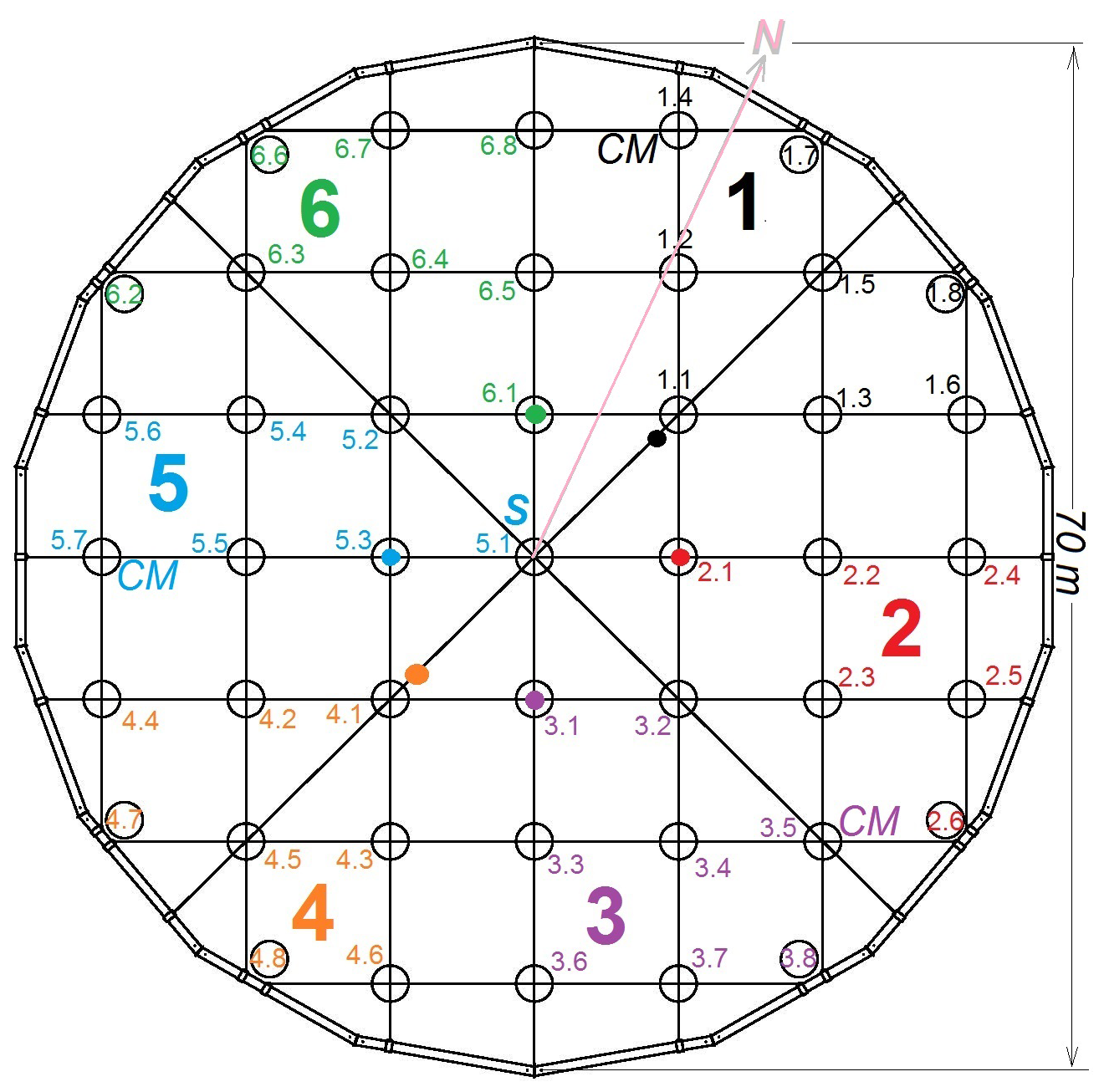
Figure A1 Orientation and layout of the large-ring mooring viewed from above, with steel-cable grid and small rings numbered in six synchronisation groups with colour dots indicating group nodes and synchroniser “S” at line 51. Here and elsewhere in the text, lines are indicated without period for short. Lines 14, 35 and 57 held a waterflow current meter “CM” at the buoy.

A2 Proposed generalization of filter cut-off to compute Ellison scales

Data from moored strings of high-resolution temperature sensors are potentially useful to compare two different manners of calculating turbulence values. The more common method proposed by Thorpe (1977) involves the reordering or sorting of unstable density overturns and the bookkeeping of their vertical displacements, for vertical profiles at each time step. Turbulence values are computed following averaging in the vertical, in time, or both and should include the largest of overturn scales. The method requires a consistent temperature-density relationship. In near-homogeneous waters, difficulties may arise in establishing such a relationship, but also in determining the size of largest overturns when they outgrow the height of the string. A method is proposed to correct over-estimation under convection turbulence by geothermal heating using verification via results from geophysical sampling (van Haren, 2025a).

In well stratified waters, the Thorpe (1977) method has been successfully compared (e.g., Itsweire, 1984; Moum, 1996; Cimatoribus et al., 2014), with results from the method introduced for atmospheric data by Ellison (1957). In this Appendix, such a comparison is done for weakly stratified waters. A modification is proposed of the Ellison (1957) method for application to data from moored instrumented strings, and which is practically based on instrument performance and environmental physics conditions.

Ellison (1957) separated time series of potential temperature θ(t,z), which is dynamically equivalent to Conservative Temperature Θ (IOC et al., 2010) in the ocean, at a fixed vertical position z in two,

$$\begin{array}{}\text{(A1)}& \mathit{\theta }=\langle \mathit{\theta }\rangle +{\mathit{\theta }}^{\prime },\end{array}$$

where 〈.〉 denotes the lpf series and the prime its hpf equivalent. If multiple sensors are deployed in the vertical to establish a mean vertical gradient, a scale height can be defined as,

$$\begin{array}{}\text{(A2)}& L_{\mathrm{E}}=\langle {\mathit{\theta }}^{\prime \mathrm{2}}{\rangle }^{\mathrm{1}/\mathrm{2}}/(\mathrm{d}\langle \mathit{\theta }\rangle /\mathrm{d}z).\end{array}$$

Itsweire (1984), using laboratory CTD-profile data, and Moum (1996), using ocean microstructure profiler data, apply sorting as filter in z-direction. While their quasi-hpf data unlikely contain (linear) internal waves, provided the profiles were instantaneously made and strictly vertical, they may contain instrumental noise. With limited time-evolution available, it is assumed that the hpf data have worked against the local stratification. The same assumption is made for Thorpe (1977) displacements. Sorting works on all scales of overturns, which can be highly varying.

Like Thorpe-displacement “d” scales, the Ellison scales of Eq. (A2) may be compared with the Ozmidov (1965) scale L_O=cL_E of largest possible turbulent overturns in stratified waters, so that the turbulence dissipation rate reads,

$$\begin{array}{}\text{(A3)}& {\mathit{\epsilon }}_{\mathrm{E}}=c^{\mathrm{2}}{L}_{\mathrm{E}}^{\mathrm{2}}{N}^{\mathrm{3}},\end{array}$$

in which the constant c needs to be established. If we take an average value of c=0.8 (Dillon, 1982), like commonly used for vertical root-mean-square “rms” Thorpe scale $L_{\mathrm{T}}=[d^{\mathrm{2}}{]}^{\mathrm{1}/\mathrm{2}}$ so that ${\mathit{\epsilon }}_{\mathrm{T}}=c^{\mathrm{2}}{L}_{\mathrm{T}}^{\mathrm{2}}{N}^{\mathrm{3}}$, one can compare average turbulence dissipation rate values between the two methods.

While the Thorpe (1977) method is most sensitive to proper resolution of the largest vertical overturn scale, and the stratification (or buoyancy frequency) it works against, determination of Ellison scales from moored-sensor time series is most sensitive for the appropriate separation between internal waves and turbulent motions (Cimatoribus et al., 2014). For data from instrumented strings under well-stratified Northeast-Atlantic conditions, wavelet decomposition worked using an averaging scale of about $\mathrm{2}/N$ for the lpf in Eq. (A1). Under such conditions, instrumental flaws like short-term bias of T-sensor data were minimal. However, such a determination of Ellison scales is not a straightforward task under weakly stratified and near-homogeneous conditions like occurring in the deep Western Mediterranean.

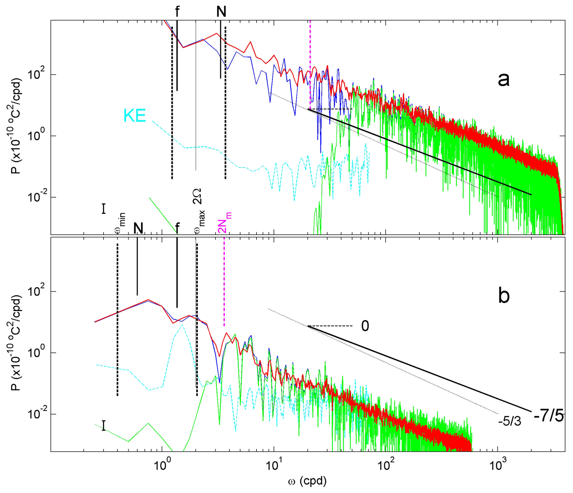
Figure A2 Spectra demonstrating filter cut-off frequencies for Ellison (1957) method under SW and NH conditions. Data from line 15. Weakly smoothed (6 degrees of freedom, dof) low-pass filtered “lpf” spectra from a single T-sensor at mid-height (thin solid) with bpf version (thin dashed) is compared with moderately smoothed (100-dof) lpf spectrum over all 63 T-sensors (thick solid). For comparison, the corresponding weakly smoothed (10-dof) kinetic energy “KE” spectra are given (thick dashed; arbitrary vertical scale), averaged over the three current meters. For reference, several frequencies and turbulence-range spectral slopes are given, see text. (a) SW period of Fig. 4, with filter cut-off following a scaling of time-mean maximum 2 m small-scale buoyancy frequency N_m and lpf cut-off at 3000 cpd (cycles per day). (b) NH period of Fig. 5, with hpf cut-off fixed near 2N_m and lpf cut-off at 500 cpd.

First, because such conditions imply very small variations in temperature (density), time series require lpf to remove instrumental noise.

Second, time series require hpf to remove internal waves and (sub-)mesoscale motions. While the common internal-wave band is considered between ranges f and N, for well stratified waters N≫f, more complex inertio-gravity wave frequency “ω” bounds [ω_min<f, ω_max>N], for large-scale mean N, have to be considered in waters where N=O(f), e.g. LeBlond and Mysak (1978) and Gerkema et al. (2008). Furthermore, while average large-scale stratification hampers turbulent overturns, internal-wave straining separates small thin-layer stratification, with small-vertical-scale buoyancy frequency N_s, from near-homogeneous layers, with minimum buoyancy frequency N_min, which may carry ditto waves extending beyond the mean-N inertio-gravity wave-bounds. At the low-frequency, sub-inertial side of the inertio-gravity wave-band the rare N_min may combine with sub-mesoscale motions. More importantly, at the high-frequency, super-buoyancy side N_s may combine with turbulent overturns. If all relevant scales are resolved, a safe separation frequency would thus be at overall maximum $N_{\text{max}}=max(max(N_{\mathrm{s}}\left)\right)$, where the maximum between brackets is determined for each profile. In practice, such a transition frequency between internal waves and turbulence is not easily determined, because it requires the small scales to resolve relevant L_O. Only in weakly stratified waters, L_O are O(10) m, and resolution of 1–2 m scales should be sufficient.

Thus, under weakly stratified conditions, instrumental noise and short-term bias have to be corrected in t- and z-direction, respectively. A practical solution that also eliminates internal waves and sub-mesoscale motions, is application of a band-pass filter “bpf” in t, an lpf and sorting in z so that per time step Eq. (A2) reads,

$$\left|{\mathit{\theta }}_{\text{bpf}}^{\prime }\right|/(\mathrm{d}{\mathit{\theta }}_{\text{sorted}}/\mathrm{d}z),$$

to which sufficient averaging is applied. Noting that stratification varies over different scales by two orders of magnitude, so that N_s≈0–6f, filter design discriminates between conditions of SW and NH. Sharp, phase-preserving double-elliptic filters (Parks and Burrus, 1987) are designed following inspection of temperature variance spectra (Fig. A2).

For SW, reasonable filter cut-offs are tuned for a 1.7 d period around day 308 by equating Eq. (A3) to ε_T. SW's lpf cut-off is fixed at 3000 cpd. The reference hpf cut-off frequency ω_hpf,ref appeared at a small flat (0-)slope near the low end of turbulence buoyancy-(${\mathit{\omega }}^{-\mathrm{7}/\mathrm{5}}$) and inertial-subrange (${\mathit{\omega }}^{-\mathrm{5}/\mathrm{3}}$) slopes, where a short steep slope to internal-wave frequencies occurred. For other SW-periods, reference is not made using average large-scale N, but a better fit is found for the time average of maximum small-scale buoyancy frequencies per profile $N_{\mathrm{m}}=\langle max\left(N_{\mathrm{s}}\right)\rangle$ so that,

$$\begin{array}{}\text{(A4)}& {\mathit{\omega }}_{\text{hpf}}^{\text{SW}}=(N_{\mathrm{m}}/N_{\text{m,ref}}{)}^{\mathrm{2}}{\mathit{\omega }}_{\text{hpf,ref}}.\end{array}$$

For NH, the lpf cut-off is fixed at 500 cpd. For its hpf cut-off, a flat (0-) slope appeared at a frequency just higher than ω_max so that, independent of measured N_m the cut-off is blocked at,

$$\begin{array}{}\text{(A5)}& {\mathit{\omega }}_{\text{hpf}}^{\text{NH}}=\mathrm{3.7}\mathrm{cpd}.\end{array}$$

This value is tuned for a period with dominant geothermal heating, for which the geophysics-determined (e.g., Pasquale et al., 1996) buoyancy flux $\text{fl}/{\mathrm{\Gamma }}_{\mathrm{C}}={\mathit{\epsilon }}_{\text{GH}}=\mathrm{1.2}\times {\mathrm{10}}^{-\mathrm{10}}$ m² s⁻³. In the present (Fig. 6) and previous (van Haren, 2025a) data the mixing coefficient was found to amount Γ_C=0.5, which is typical for convection turbulence (Dalziel et al., 2008; Ng et al., 2016).

The cut-off frequency in Eq. (A5) is to within ±0.2 cpd equivalent to $\mathrm{1.8}\left(\mathrm{2}\mathrm{\Omega }\right)\approx \mathrm{1.8}\langle {\mathit{\omega }}_{\text{max}}\rangle \approx \mathrm{2}{N}_{\mathrm{m}}\approx \mathrm{0.5}\langle U\rangle /\langle L_{\mathrm{T}}\rangle =\mathrm{0.5}{\mathit{\omega }}_{\mathrm{O}}$, for the deep Western Mediterranean site. Ω denotes the Earth rotation, and U the waterflow speed. The Ozmidov (1965) frequency ω_O is a natural separator between internal waves and stratified turbulence. It is unknown why the filter cut-off is close to half the Ozmidov frequency. Also puzzling is the lack of correspondence between Eq. (A4) and ω_O, with the factor varying between 0.3 and 0.9 for different periods of SW. In part this may have to do with the waterflow being measured at h=126 m, below which it may be more uniform under NH- than under SW-conditions.

As shown in Fig. 4 for Eq. (A4), and Fig. 5 for Eq. (A5), the comparison between average turbulence dissipation rate values using Ellison (1957) and Thorpe (1977) methods works well to within a relative error of about 20 % of the mean value. To Fig. 4, $\langle \left[{\mathit{\epsilon }}_{\mathrm{T}}\right]\rangle =\mathrm{6.3}\times {\mathrm{10}}^{-\mathrm{10}}$ m² s⁻³ and $\langle \left[{\mathit{\epsilon }}_{\mathrm{E}}\right]\rangle =\mathrm{6.7}\times {\mathrm{10}}^{-\mathrm{10}}$ m² s⁻³. To Fig. 5, $\langle \left[{\mathit{\epsilon }}_{\mathrm{T}}\right]\rangle =\mathrm{2.0}\times {\mathrm{10}}^{-\mathrm{10}}$ m² s⁻³ and $\langle \left[{\mathit{\epsilon }}_{\mathrm{E}}\right]\rangle =\mathrm{1.3}\times {\mathrm{10}}^{-\mathrm{10}}$ m² s⁻³. Further tests were performed for about ten 1–4 d periods of NH and SW, and all were within above relative error, provided that the data post-processing was carefully done and longer periods were avoided. Especially Eq. (A5) is very sensitive to small changes in filter steepness around the cut-off frequency, presumably due to its proximity to the inertio-gravity wave upper bound.