
the Creative Commons Attribution 4.0 License.
the Creative Commons Attribution 4.0 License.
 | 27 May 2026
Monitoring surface gravity wave variability with State of Polarization sensing on a subsea telecommunication cable
Julián D. Pelaez Quiñones
Steinar Bjørnstad
Peter J. Thomas
Per Lunde
State of polarization (SoP) sensing is a fibre-optic interrogation technique that recovers cumulative polarization variations of probe lasers transmitted between opposite ends of optical fibres. These changes can be triggered by various external stimuli interfering with the guided light in the fibre, including surface gravity wave-induced motions, as evidenced by prior studies. In this study, we advance this knowledge by quantitatively assessing the capacity of SoP sensing to continuously capture surface gravity wave height and frequency variability in the ocean along a subsea telecommunication cable via comparison with reference in situ and validated model data. Our SoP dataset consists of nearly 11 months of data collected at the landing site of a ∼240 km back-looped fibre link across the Norwegian trench over the North sea, between the city of Egersund in the Southwestern coast of Norway and an offshore bottom-fixed platform. Spectral and correlation analyses demonstrate the capacity of SoP to detect both, wind waves and swells acting simultaneously over different regions of the cable in the 0.03–0.6 Hz range. During the observation period, wind waves affected mostly the offshore end of the cable, while swell signatures dominated in the coastal region, close to the landing site. Correlation coefficients of up to nearly 70 % are obtained between SoP data and the wave analysis model for the full observation period. We discuss various physical aspects related to the SoP measurements and outline some of their limitations for sea state monitoring, chiefly in terms of interpretation capacity and sensitivity. Our results also evidence that SoP sensing systems can be a practical way to obtain dynamic, first-order estimates of the sea state variability where cables are sufficiently shallow. A non-negligible portion of the extensive infrastructure of submarine telecommunication cable networks has thus the potential to be turned into arrays of remotely-operated sensors of opportunity that are complementary to well-established oceanographic instruments.
- Article
(12052 KB) - Full-text XML
- BibTeX
- EndNote


The monitoring of ocean waves and marine storms is a topic of growing importance due to the effects of climate change, with some projections hinting at an increased severity and geographical coverage of extreme marine weather events, most notably tropical and extratropical cyclones (Kossin et al., 2014; Mann et al., 2017; Chang, 2018; Kossin et al., 2020). At the same time, the monitoring of ocean waves is a topic of permanent scientific interest due to the role of the sea state in the ocean-atmosphere feedback system. Major interests in monitoring the sea state also stem from the increasingly widespread human use of, interaction with, and profit from the oceans. Modern technological offshore developments such as renewable energy converters and storage, maritime navigation and other marine infrastructure can thus benefit from (real-time) information about the sea state. Furthermore, populated coastal areas are becoming increasingly exposed to the erosional effects of large ocean wave events due to sea level rise, in a way that early warning and protective infrastructure systems against storm surges and tsunamis can always benefit from existing and robust sensors providing remotely-operated and real-time monitoring opportunities with optimal coverage.
State of polarization (SoP) sensing is a fibre-optic (FO) sensing technique that relies on the monitoring of the polarization state of a laser received at one end of an optical fibre link (Namihira et al., 1988; Zhan et al., 2021; Mecozzi et al., 2021; Pellegrini et al., 2025). The light source on the opposite end only needs to be continuous in time, sufficiently intense for the optical detector at the receiver end to yield good signal-to-noise (SNR) after attenuation through the fibre, and ideally having stable (or controllable) input polarization. Birefringence variations in the optical fibers induced by environmental perturbations dominate the SoP signal (Mecozzi et al., 2021). This birefringence arises from strain-induced anisotropy, i.e., differential changes in the refractive index along orthogonal axes of the fiber. These anisotropic perturbations lead to relative phase (or time) delays between light components oscillating along different polarization axes, ultimately resulting in a net evolution of the SoP as the environmental physical conditions change. The transmission architecture means that the technique is two-ended and can rely on conventional FO laser sources (used for internet data traffic), with no requirements of complex, highly coherent or short pulse laser signals.
SoP provides a single integrated measurement per temporal sample (e.g. the entire fibre link or looped fibre segments between repeaters) that is generally cross-sensitive to (sufficiently strong) mechanical strains, temperature changes and strong electromagnetic fields (e.g. lightnings or high-voltage lines) interacting with any section of the fibre (Fang et al., 2012; Hartog, 2017), so that its spatial sampling distance equals the arc-length path occupied by the interrogated fibre link. If the SoP source and receiver are located at opposite ends of a cable, the measurement integrates over the entire fibre length. In subsea systems employing loop-back configurations, the effective spatial resolution corresponds to half the total loop length (i.e. the full cable length, as in our experiment). Some modern SoP systems can achieve a better spatial resolution matching the separation between cable repeaters (amplifiers) with high-loss loop backs (Marra et al., 2022; Yaman et al., 2025) that are typically 50–120 km apart for long, submarine transoceanic cables, and have attenuation losses at ∼20 dB.
In this work, we investigate in detail the capacity of offshore SoP systems to continuously monitor ocean waves, (i.e. surface gravity waves (SGW), Massel, 2017). Theoretical developments and proof of the capacity of SoP systems to detect ocean waves with subsea cables were presented in e.g. Mecozzi et al. (2021), Zhan et al. (2021), and Mecozzi (2024). However, these studies lacked ground truth validation to ascertain and quantify the degree of spatio-temporal correlation between the detected SoP anomalies and particular ocean wave events along the stretch of their cables. Here, we intend to tackle these gaps by performing a multiparametric correlation analysis between continuous SoP measurements over the course of several months and a validated ocean wave analysis model (Ardhuin et al., 2010), thus accounting for the accuracy and reliability of SoP to detect and monitor surface gravity wave height variability with typical, subsea telecommunication cables which were not originally intended for such purposes. Reference in situ oceanographic measurements are also included to further validate the model output and the SoP observations. Temporal and spectral analyses confirm that SoP signals in the 0.03–0.6 Hz range are predominantly related to the influence of surface gravity waves acting upon the cable. The presence of swells, wind waves, and specific storm events on the SoP data are highlighted, and the capacity of the system to monitor ocean waves over several months is evaluated and discussed.
While our study focuses on the detection of ocean gravity wave height variability, we emphasize the capacity of SoP systems to detect numerous physical forcing mechanisms, both on- and offshore, including, but not limited to: seismic monitoring (Dejdar et al., 2021; Zhan et al., 2021; Costa et al., 2023; Carver and Zhou, 2024), lightning detection (Charlton et al., 2017), and wind anomaly detection with aerial cables (Wuttke et al., 2003). Furthermore, recent advances highlight the potential of the more popular single-ended, distributed FO systems such as Distributed Acoustic Sensing (DAS) to monitor gravity waves at high spatial resolutions using the same conventional optical fibres as well as other oceanographic phenomena (see Wei et al., 2024, for a review on the topic). Overall, the former studies and the present one provide evidence for the potential of subsea cable networks as remotely-operated sensors of opportunity to monitor the sea state in real-time and contribute to the pool of available in situ oceanographic devices.
The text is divided as follows. Section 2 compiles fundamental aspects of SoP sensing. Section 3 describes the experimental set-up and the data used in the work. Section 4 presents the main results, including temporal, spectral and correlation analyses of SoP measurements with reference data. Results are discussed in Sect. 5, followed by a concluding remarks section, Sect. 6.
The SoP of a light beam can be expressed in a variety of ways, a common one being the Stokes vector , whose parameters are relatively simple to measure and represent altogether the instantaneous polarization of the electric field of an electromagnetic wave propagating along a fibre whose axis is oriented in the z-direction (e.g. Yin, 2002; Fang et al., 2012):
where δ represents the relative phase shift between the electric field components on a reference orthogonal basis perpendicular to the direction of propagation. A common 3D representation of these states is the so-called Poincaré sphere, defined by S1, S2 and S3 as orthogonal basis, being proportional to the beam intensity and implying that only three out of the four parameters are mutually independent. In this work, only the S1 parameter will be addressed.
For an input light beam guided into a fibre link of length L, the time-dependent polarization variations of the output beam can be expressed by a Stokes vector s whose value is related to the accumulated birefringence variations along the fibre range z, as outlined by Eq. (6) in Mecozzi et al. (2021),
where represents the spatio-temporal variations of the fibre birefringence matrix (β) component perpendicular to the input beam Stokes vector under a reference frame rotating along with the static birefringence of the fibre (Mecozzi, 2024). This unperturbed state is in turn defined by its degree of anisotropy, naturally resulting from its quasi-static mechanical state (e.g. tension, torsion and bend) as well as the random fibre core internal structure heterogeneities (e.g. lattice defects and cleavage) imprinted during manufacture.
Assuming that the input SoP remains constant, the fluctuations observed in the SoP measurements are directly related to the accumulated contribution of birefringence variations along the fibre link caused by external physical perturbations interacting with the fibre (Hartog, 2017), including those induced by sufficiently strong noise sources nearby e.g. dynamic strain, temperature, torsion and bending. If large enough, such forces are capable of differentially changing the refractive index of the fibre (via photoelastic effect) across the radial plane of the fibre. As a result, the propagation speed of light modes having different polarizations will generally change at uneven proportions under the same forcing mechanism acting on the same fibre section, thus generating a spatio-temporal dependent δ that generally affects all Stokes parameters simultaneously. A key implication arising from the 3-dimensional rotation and drift of the Stokes vector along the Poincaré sphere when responding to external stimuli is that a single Stokes parameter cannot be assumed to always linearly represent the intensity of the stimulus itself, as will be discussed later in the text.
3.1 State of Polarization system
The implemented SoP system is sensitive to variations in both the optical power and the polarization orientation of the received laser beam and was designed to analyze the S1 Stokes parameter alone owing to design simplicity and low cost. Thus this work will exclusively focus on this parameter. At the receive fibre end, a polarizing beam splitter (PBS) separates the beam into two orthogonal polarization components whose power is proportionally converted into voltages with photodiodes and sampled with an analog-to-digital (ADC) converter (Barcik and Munster, 2020; Skarvang et al., 2023; Bjørnstad et al., 2024). As the squared electric field is proportional to the optical power received by SoP (which is then converted into voltage), the normalized voltages () from the two PBS channels can be subtracted to obtain a proxy for the S1 Stokes parameter of Eq. (1). However, because the implemented ADC is AC-coupled (only alternating variations are measured, as opposed to absolute levels) and the relative attenuation of the photodiode detectors has not been properly calibrated, this proxy rather represents a first-order estimate of relative changes of S1 over time and we will thus refer to it as . Note that S0 describes the (nearly constant) intensity of the input laser, yet since the detectors are not balanced, some SoP variations would unpredictably leak into S0 if estimated via addition of the two PBS channels.
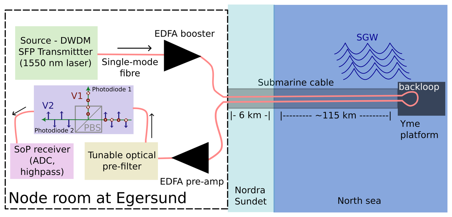
Figure 1Set-up component diagram (based on Bjørnstad et al., 2024).
Figure 1 shows a schematic diagram of the set-up. The laser beam on the transmitter fibre end is polarization stable, has a wavelength of 1550 nm (typical low-attenuation laser in fibres). A continuous wavelength-specific DWDM (Dense Wavelength-Division Multiplexing) small form-factor pluggable (SFP) device is used as laser source. An EDFA (Erbium Doped Fibre Amplifier) having a flat, broadband noise spectrum boosts this carrier wave to 16 dBm prior to entering the fibre link. After traveling through the entire link, the received signal is pre-amplified with another EDFA and then pre-filtered with a tunable optical filter (matched to the transmitted wavelength) to reduce widespread ASE (Amplified Spontaneous Emission) and electronic noise from the optical amplifiers, reaching −11 dBm upon entering the polarizing beam splitter (PBS). The PBS splits the incoming light in two orthogonal components that are routed to separate optical detectors (photodiodes) that convert electromagnetic (EM) power into voltages. The ADC (analog-digital converter) sampled at 44.1 kHz and has a built-in digital high-pass filter with +10 dB per decade in frequency (first-order) linear gain roll-off in the SGW band (0.01–1.0 Hz) which was compensated for in preprocessing with a Butterworth low-pass filter of the same order (−10 dB per decade) to keep the spectral response flat in that band.
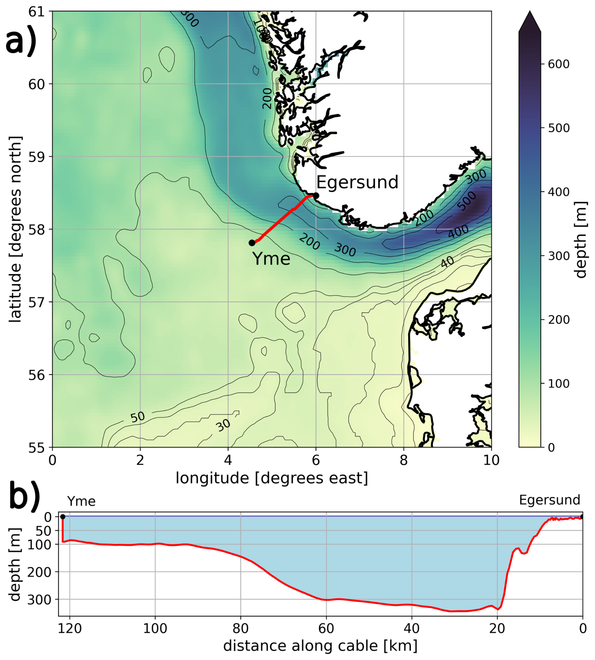
Figure 2(a) Subsea cable bathymetric layout in the North sea between Egersund (SW Norway) and the Yme offshore platform. (b) Horizontal profile of the cable along the bottom. Bathymetry obtained from E.U. Copernicus Marine Service Information (https://doi.org/10.48670/moi-00055, Bruciaferri et al., 2021).
Nearly 11 months (1 June 2023 to 26 April 2024) of SoP data, decimated to 5 Hz for manageability, are analyzed. In total, there were less than 3 h of gaps during the entire observation period. The FO link consists of a 240 km-long U-looped dark fibre pair inside a (120 km) double armoured subsea cable (ca. 3 cm in diameter) spanning between a sheltered node room in the coastal town of Egersund, Norway, and the Yme hydrocarbon extraction platform in the North Sea ( N, E) located nearly 100 km from Eigerøy, the closest point in land just by the landing section of the cable (Figs. 1 and 2a). The map data was obtained from https://doi.org/10.48670/moi-00055 (Bruciaferri et al., 2021). The other fibres in the same cable were allocated for telecommunication purposes. The cable follows a nearly straight horizontal projection averaging 047227 azimuth degrees between these end points and remains mostly buried between 1 to 2 m under the sediments, with only a few sections exposed to water. The region coincides with a major amphidromic point in the North Sea (Sündermann and Pohlmann, 2011). As the cable reaches the location of the platform at Yme (at approx. 90 m water depth, Fig. 2b), it is cased along a metallic J-tube permanently attached to the jacket of the platform (the subsea support tower fixed to the seabed) and rising nearly vertically from the bottom and into the platform passing through the water surface. As the fibre link is looped-back at the Yme platform, the SoP transmitter and receiver are co-located in the same node room at Egersund. The sensing end of the fibre is spliced to a buried FO extension in a manhole next to the node room. The latter is located next to a road, less than a hundred meters from the shore of the Nordra Sundet fjord next to Egersund. This sheltered and shallow inlet (<10 m deep on average) connects with the North sea upon reaching the Nordragabet bay after nearly 6 km from the landing site.
3.2 Ocean wave analysis model data
In order to compare the SoP measurements with spatially resolved reference data, we used a regional implementation of the MFWAM (Meteo France WAve Model), a validated, hourly spectral wave analysis and forecast (Ardhuin et al., 2010) on the Atlantic-European North West Shelf area (16° W–10° E; 46–61.3° N). The data were obtained from the E.U. Copernicus Marine Service Information; https://doi.org/10.48670/moi-00055 and Bruciaferri et al. (2021). The model is forced by wind data from ECMWF (European Centre for Medium-Range Weather Forecasts) and currents by the IBI-MFC (Iberia Biscay Irish – Monitoring Forecasting Centre) ocean circulation system. Wave height altimeter and directional wave spectral data from Sentinel1-A and CFOSAT (Chinese-French Oceanography Satellite) are assimilated with an optimal interpolation scheme (Lionello et al., 1992). The geographical resolution of the model is 0.03° (each spatial sample covers ∼11 km2). Wave directional spectra covers the 0.035–0.56 Hz band and are discretized in 24 directions. Significant wave heights are calculated as four times the standard deviation of the surface elevation spectrum (HM0) and have root mean square (RMS) deviations below 0.3 m. The wave model peak energy partitioning technique splits the full wave spectrum into significant wind wave (HM0WW) and swell (HM0SW) height components. These typically cover the high and low frequency portion of the wave spectrum, respectively. Swells are further divided into two sub-components (primary and secondary, based on their relative prominence). The model variables relevant to this work are listed in Table A1.
3.3 In situ reference data
Point-measurement data from oceanographic sensors at the Yme platform is used as ground truth to provide fine-detail, complementary information about the observed SGW variability and confirm the reliability of the different wave model parameters in the particular study region. A Fugro Seawatch Wavescan buoy anchored to the north of the platform provides current direction, mean wind direction and mean wave direction. The waveradar is a Saab Waveradar Rex mounted on the platform and located 54.3 m above mean sea level. The in situ significant wave height data (*HM0) is a combination of readings from these two sensors as a single time series (cf. the Norwegian centre for climate services, https://seklima.met.no/, last access: 20 May 2026) and is further subdivided into significant wind wave and swell height contributions (, respectively). All parameters used in this work were originally sampled at 10 min intervals. Table A1 presents an overview of all the in situ wave parameters used in this work. The mean location of this station (local code SN76929, WIGOS number 0-578-0-76929) is 57.82 N, 4.54 E.
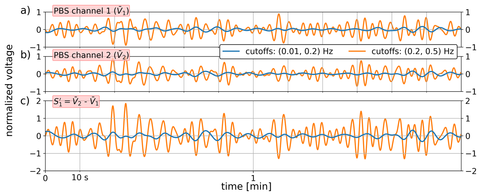
Figure 3Sample measurement of the two PBS receiver channels of the SoP instrument (a, b), band-pass filtered (zero-phase 4th-order Butterworth) at low (blue) and high (orange) frequency bands. Panel (c) depicts the subtraction of the two signals, here referred to as .
4.1 Temporal and spectral series
To illustrate how the signal is obtained, Fig. 3 depicts two minutes of PBS channel voltage signals (here band-pass filtered at two frequency bands only for illustration purposes). These signals are subtracted to obtain a proxy for S1 (Eq. 1 and Fig. 3c, here named as explained in Sect. 3). Coherent signals with periods of a few seconds are present in both channels with opposite phases, thus amplified upon subtraction. Signals will tend to have larger values in either of the (randomly oriented) PBS channel axes as the received instantaneous polarization of the optical carrier aligns closer to either axis. Since the relative amount of signal distributed between both PBS channels will fluctuate with a magnitude and period proportional to that of the external forcing (e.g. SGW), the time series thus contains a signature of the spectral characteristics of the external forcing.
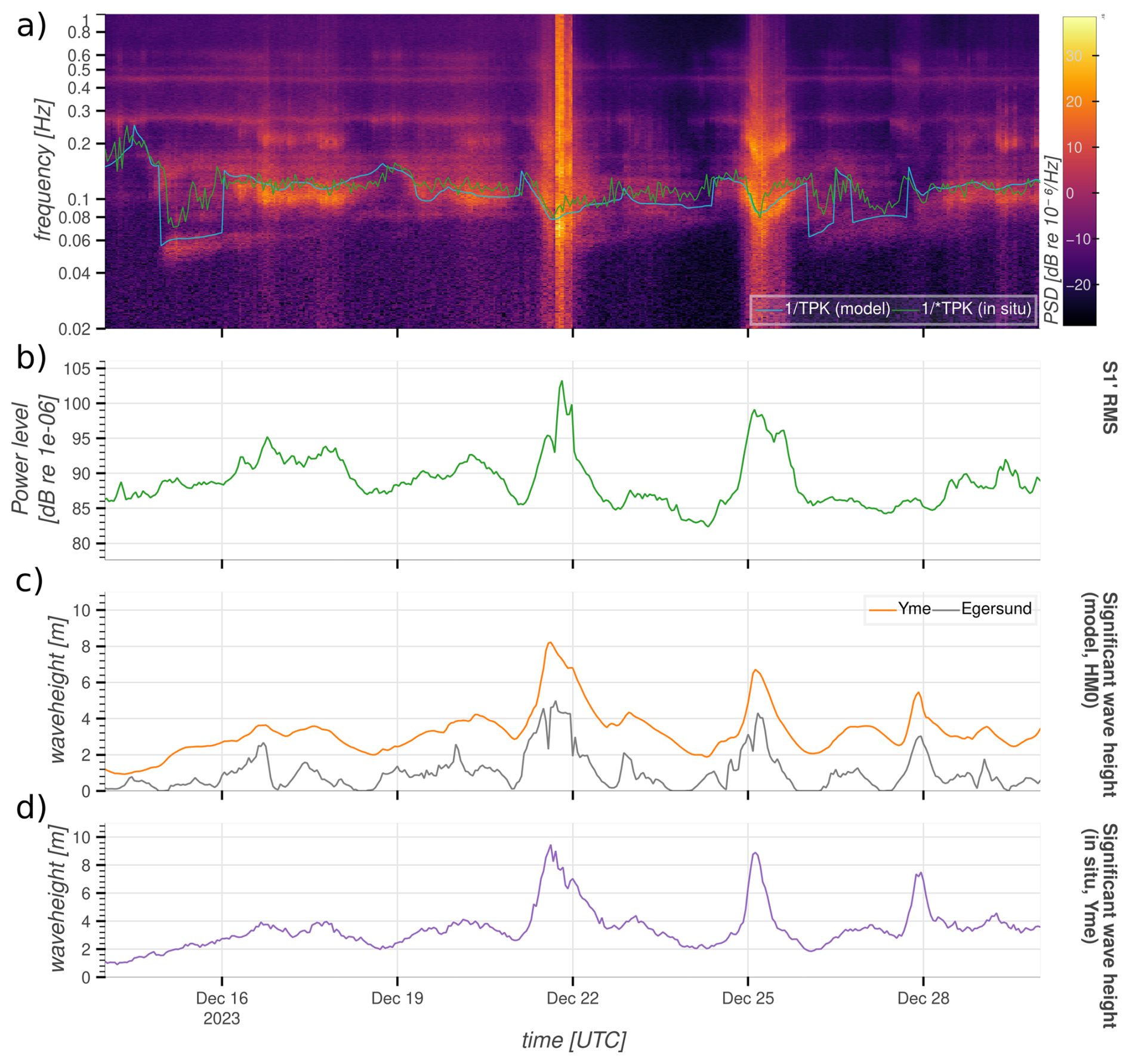
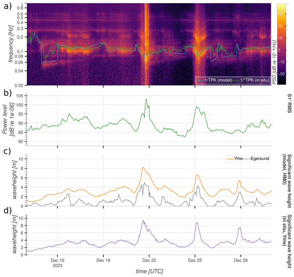
Figure 4Power spectral density (PSD) spectrogram of with modeled dominant wave frequency curves at Yme overlaid (a); hourly RMS of the measured SoP () time series (b); wave height analysis model at the Egersund coast and Yme (c); and wave height in situ measurements at Yme (d). Starred (*) parameters refer to in situ data, otherwise to wave analysis model. See Table A1 for a description of all the ocean parameters used in this work.
As an example, a two-week comparison of the temporal and spectral series of , the significant wave heights from the wave analysis model at two of the shallow-most locations at the near-shore and offshore ends of the cable (Egersund and Yme, respectively), and in situ wave height measurements at Yme, are presented in Fig. 4. The choice of these particular locations will become clearer in the following sections.
The power spectral density spectrogram of Fig. 4a shows prominent spectral energy features, some transient with a broadband character (e.g. the peaks on 22 and 25 December), others spread in time over narrower bands (e.g. the event between 16–19 December). Both are likely to correspond to surface gravity wave (SGW) energy peaks induced during marine storms, as evidenced by the events on early 22 and 25 December having characteristic upwards “V-shaped” spectral energy distributions in the frequency range 0.05–0.5 Hz, typical of the onset and coda of SGW induced by wind storms (e.g. Ferretti et al., 2013; Colosi et al., 2023). evidences a stable, modulated (in frequency and amplitude) background line spectrum above about 0.08 Hz that is commonplace to the entire dataset and likely to be linked to optical transmitter noise. A first-order harmonic around 0.2 Hz akin to mechanical resonance is present during the 22 and 25 December events. An overall good correlation between the spectral power distribution of and the dominant period variability of the wave model (surface wave full-spectrum – TPK, wind waves – TM01WW, and primary swells – TM01SW1 spectral peaks) and the in situ sensors at Yme (full-spectrum – *TPK, wind waves – *TWW, and swells – *TSW spectral peaks) further evidences the capacity of SoP to measure both wind waves and swells (cf. Table A1 for a description of these parameters). Most of the spectral signatures below about 0.5 Hz populating the spectrogram of Fig. 4a correlate to variable degrees with any of the aforementioned reference frequency parameters. Notably, within 15–17 December a low-frequency swell with a normal dispersion trend typical of SGW is evident in that partially matches the model peak frequency, TPK−1 (Fig. 4a). However, its coda (lasting until 17 December) is neglected by both the wave model and the Yme in situ sensor, such that its duration would have been interpreted incorrectly without high sampling rate spectral data. The spectral noise energy modulations of SoP tends to match the fluctuations in , in a way that wind waves of higher frequency (typically of decreasing amplitude) are generally related to reduced energy and vice versa (Fig. 4a). It is worth noting the significant fading in spectral energy on the spectrogram at lower frequencies, particularly below 0.05 Hz.
To derive a metric proportional to the energy of the SoP signal, the hourly root-mean-square (RMS) of was computed in the time domain by applying 1 h non-overlapping windows to the bandpass-filtered (0.03–0.6 Hz, fourth-order Butterworth) squared time series (Fig. 4b). Most SGW energy is generally confined in this band, 0.03 Hz approximating the boundary between typical SGW and the infra-gravity wave domain. The resulting hourly RMS values were then compared with the modeled wave heights, which serve as a proxy for wave energy (Fig. 4c). These curves illustrate an overall similarity between the power level of the SoP signals (in dB scale relative to a randomly chosen small value) and the significant wave heights at both ends of the cable, although with noticeable sporadic deviations. The upper filtering limit was set to avoid high-frequency line spectrum noise unrelated to SGWs (Fig. 4a). A qualitative validation of these trends is presented in Fig. 4d, which shows the in situ significant wave heights at Yme and evidence a good fit with the hourly model of Fig. 4c albeit the shorter-term variability absent in the latter, as well as a positive correlation with the hourly (Fig. 4b). The wave activity at Yme is larger most of the time, though most wave height anomalies are represented similarly in both time series since the surface wave spectrum usually varies smoothly in space. From Fig. 4a, the maximum SNR ratio of relative to the background floor is about 30 dB, averaging at 11 dB over the full SGW band.
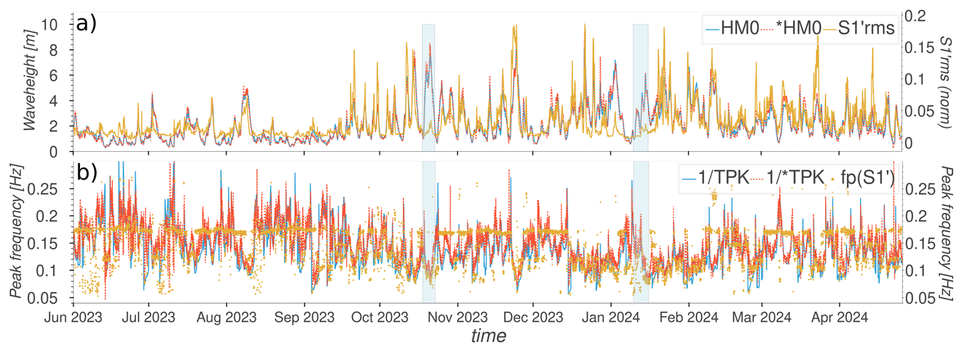
Figure 5Full observation time series SoP and reference data. (a) Significant wave heights from model (HM0) and in-situ sensor (*HM0) at Yme compared to the normalized hourly RMS of (with extreme outliers above the 99th percentile trimmed off). (b) Peak frequency from model (TPK−1) and in-situ sensor () at Yme compared to the hourly peak frequency fp of in the range 0.05–0.25 Hz.
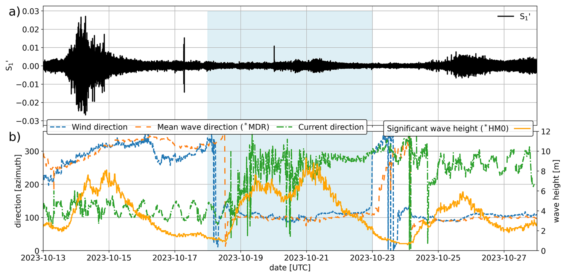
Figure 6 time series band-passed in the 0.03–0.6 Hz range (a) and concurrent in situ measurements at the Yme platform (b) during sea storm activity. The area shaded in blue depicts a major wave event undetected by SoP.
Figure 5a depicts the entire normalized, hourly RMS time series of alongside the in situ (*HM0) and modeled (HM0) significant wave heights at Yme. It illustrates the general degree of correlation between and the wave heights, and evidences that most wave events are represented in the series, with the exception of a few energetic events that are poorly detected by SoP (e.g. 18–23 October 2023 and 10–16 January 2024), as previously noted in Sect. 4.1 (Fig. 6) and marked by blue-shaded time spans in Fig. 5a and b. The peak frequency of estimated over hourly time windows is shown in Fig. 5b and only evidences a moderate match with the reference data values, with errors being above a quarter of the considered bandwidth in at least 20 % of the observations. Correlations are slightly better at lower frequencies during the more SGW-energetic winter season, while deviations become more marked during the Summer low in SGW activity. The 0.17–0.18 Hz constant peak is unrelated to SGW activity and corresponds to one of the dominant components of the modulated SoP noise line spectrum previously evidenced from Fig. 4a. This instrumental noise is dominant during nearly half of the entire time series and is capable of intermittently obscuring the weakest SGW signals, significantly biasing peak frequency estimates.
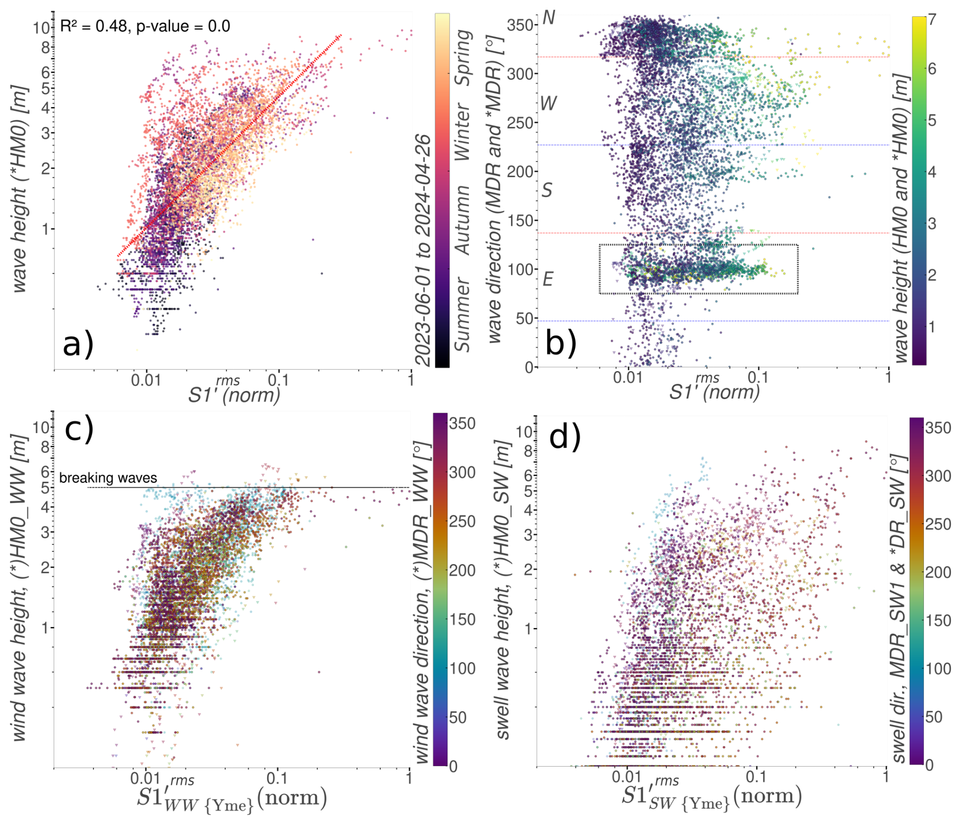
Figure 7Bivariate plots of the hourly RMS of and various reference wave parameters at Yme in log-log scale: (a) in situ significant SGW height *HM0 (time in color scale) with linear regression (including determination coefficient R2 and p-value of t-distribution Wald test for zero vs. positive slopes hypotheses,); (b) in situ mean wave direction *MDR (data gaps filled with modeled data, MDR). In situ significant wave height, *HM0, in color scale (gaps filled with HM0). Blue (red) lines are parallel (normal) to the mean azimuth of the entire cable; (c) in situ significant wind wave height *HM0WW (data gaps filled with HM0WW). In situ mean wind wave direction, *MDRWW, in color scale (gaps filled with MDRWW); and (d) in situ significant swell height *HM0SW (gaps filled with HM0SW). In situ swell direction, *DRSW, in color scale (gaps filled with MDRSW1). All modeled data points are indicated by triangles. and are the estimated wind- and swell-induced SoP signals, as introduced in Sect. 4.3.
Interestingly, some major SGW anomalies went virtually undetected in the SoP signal, e.g. between 18–23 October 2023 and 10–16 January 2024 (shaded regions in Fig. 5a). At the onset of the first of the aforementioned timespans (shaded region in Fig. 6b), a synchronous, major shift in the mean surface wave and near-surface current directions at Yme took place, likely triggered by a ∼160° change in the wind direction regime towards 100° azimuth. Notably, the measured ocean currents shifted from a steady (roughly SEE), tide-modulated regime to a more chaotic, short-period azimuthal fluctuation likely reflecting extreme movement of the measurement buoy and during which the major SGW event barely triggered a noticeable response. Contrastingly, the in situ SGW variability before and after this event do seem to trigger prominent anomalies. A similar observation will be presented in Fig. 7b.
4.2 Bivariate correlations
To quantify the degree of similarity between the trends of the SoP measurements and the true wave heights observed in the previous sections, a bivariate analysis of the full time series follows. Figure 7a shows a bivariate scatter plot between the hourly RMS of and the in situ significant wave height at Yme (*HM0), where the largest wave height anomalies are expected from the observations in Sects. 4.1 and 4.3. The yearly season is indicated by the colormap. SGW activity was largest between fall and early spring, with some energetic wave events coinciding with less prominent anomalies during winter (later December to mid-January, as evident from Figs. 7a and 5a). A linear regression between both variables shows a positive correlation with a determination coefficient at 48 % resulting from the large amount of scatter between the variables, and evidencing a moderate-to-low degree of correlation between the true wave heights at Yme and . On the other hand, hints of a slightly non-linear component in Fig. 7a are also apparent (see Fig. C1 for further statistics from the regression). The multiple branches and sub-clusters of points evidence a non-trivial correlation between the SoP response and the ocean wave energy.
Two major in situ mean wave direction sub-clusters (*MDR; with MDR data points indicated by triangles where in situ data gaps occur) are observed in Fig. 7b, towards the NNW (around 350°) and SEE (around 100°, delimited by black box), showing that although there is an overall positive correlation between the RMS and significant wave heights for most azimuths, there are also preferential wave directions that break-up this correspondence (especially events directed towards the 100° azimuth cluster). A slight tendency of waves towards the NNW (310–360°) coinciding with smaller SoP anomalies than the other directions is also present. Most SGW in the observation region tend to be oriented westwards, evidencing that the wavefield was not omnidirectional during the observation period. The blue and red lines in Fig. 7b mark the overall azimuth of the cable and its perpendicular.
An accurate separation of the wind and swell wave contributions to ( and , respectively) would require a so-called wind-swell separation frequency, fs(t), which theoretically lies between the peak frequencies of the wind and swell components (as evident from Fig. 4a) and formally demands wave moment calculations from the full SGW spectrum (Hwang et al., 2012). However, as the best approximation for such data is the 10 min peak wind and swell wave periods at the Yme in situ sensors are available (, which are in fact derived from the full spectrum), an empirical approximation of fs is here calculated as . The hourly RMS of and can thus be estimated to first-order by integration of the hourly PSD spectra of across the bands [0.03-] and [-0.6] Hz, respectively. Figure 9i will later confirm that the mean throughout the full observation period has a relatively homogeneous spatial distribution over the whole cable, thus validating the calculation of this proxy from data at Yme.
A slight non-linearity in the correlation trend is hinted by Fig. 7c that resembles that observed in Fig. 7a. The former plot correlates the hourly RMS of with the hourly wind wave heights of the situ sensors *HM0WW (in situ data gaps filled with the wind wave component of the model, HM0WW and depicted with triangles). Qualitatively, the data point trends of the wind component show a similar random scatter and trend as that of the full-spectrum case (Fig. 7a). Data points at wind wave directions (*MDRWW) outside the 50–150° range (covering the same anomalous cluster of points of Fig. 7b around 100° inside black box) are plotted in blue tones with higher transparency in Fig. 7c. This sub-cluster shows some deviation from the main data point cluster, with large wind wave height that seem to generate very subtle SoP responses. The wave height limit depicted at 5 m in Fig. 7c is related to breaking waves at Yme and was obtained from a comparison between the wind wave component measured at Yme and that estimated by the wave model (see Appendix D and Fig. D1b and c). This cut-off explains to some degree the observed non-linear trend at high wave height values. The horizontal arrangements of dots in the lower parts of Fig. 7c and d results from the measurement resolution limit of the in situ sensor.
A more scattered correlation trend exists between the hourly RMS of and the in situ swell component at Yme *HM0SW (Fig. 7d, with in situ data gaps filled with HM0SW model values and depicted by triangles with higher transparency). Although there is a generally positive correlation, a marked random tendency is evident from the significant scatter. No wave breaking limit cut-off effect is evident for swell waves and no obvious correspondence exists between the point scatter trends and the directional component of the swell (*DRSW; MDRSW used where in situ data gaps occur).
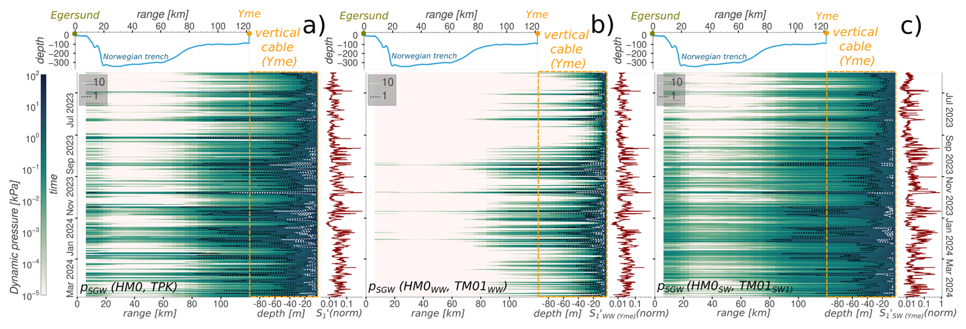
Figure 8SGW-induced dynamic pressure variability estimated for the significant full-spectrum (a), wind wave (b) and swell (c) wave height components over the cable, depending on its depth (shown on top of each panel). The maximum-normalized hourly RMS of is shown on the right of each panel for (a) the full spectrum (0.03–0.6 Hz, ), (b) wind () and (c) swell () wave components of , as calculated from its hourly spectrum based on in situ measurements at Yme (see text for details). The delimited region corresponds to the vertical cable segment between the seafloor and the surface at Yme. Pressure values and dashed contours (labels in grey box) in kPa.
The regression slope of Fig. 7a leads to a first-order estimate of the (linear) relative sensitivity of the RMS of to significant wave height variations of 0.017 % m−1 (relative to the dynamic range of the instrument) for the cable link under study, with a large standard deviation at 0.008 % m−1. It should be outlined that this is likely an overestimate, given the expected additional contribution to the observed SoP variability from wave energy into other cable segments farther apart from Yme, including the seafloor cable segment over the shallow North Sea and the landing end at Egersund (Fig. 8).
From Fig. 7a, the threshold RMS values below which correlations with wave heights are no longer evident lies at about 1 % of the observed maximum and corresponds to the mean of the 10th percentile of . This threshold also corresponds to observation times with wave heights below 1 m, such that the reliable recovery of small wave heights below this limit for the investigated fibre link is compromised and can thus affect correlations during times of very low SGW activity.
4.3 Modeled peak variability along the cable
As each SoP sample is an integrated measurement along the full extent of the backlooped fibre, it is not yet clear which specific sensitive segment(s) act(s) as antenna(s) for the detected SGW variability. As SoP is sensitive to strains on the fibre, the pressure gradients induced by SGW upon the cable are expected to play an important role in generating the observed variability. To shed light on this, Fig. 8a–c depict distance-time plots along the full cable extent for nearly six months of data, both for the cable section on the seafloor, as well as the tubed vertical segment reaching the water surface just below the Yme platform. The main variable plotted here is the expected absolute dynamic pressure induced by SGW, pSGW(k,z) (Eq. B1) exerted on the corresponding cable segment depending on its depth z, wavenumber k, and the modeled significant wave height component on top of it for: (1) the full-spectrum (HM0, Fig. 8a), (2) wind waves (HM0WW, Fig. 8b) and (3) swells (HM0SW, Fig. 8c). The corresponding representative wave period parameters () are also required for each plot because the vertical attenuation of SGW is frequency-dependent and is thus also implemented in the calculation of the depth-dependent pressure based on the linear wave approximation (cf. Appendix B and Fig. B1). In the case of swells, instead of averaging the mean periods of the two most prominent spectral components from the model (TM01SW1,TM01SW2), only the mean period of the largest swell is implemented. Note that in Fig. 8a, TPK designates the peak period over the full SGW spectrum so that pSGW(HM0,TPK) is thus variably biased towards swells or wind wave activity depending on the changing sea state. At the same time, even if having smaller heights than wind waves, the excess pressure of swells tends to penetrate into deeper waters owing to their larger wavelengths.
For comparison, the maximum-normalized hourly RMS signals estimated in the frequency bands corresponding to that of each of the SGW model components are also shown at the right side of each panel in Fig. 8.
Based on the pressure signal derived from the full spectrum, Fig. 8a confirms that the two shallower ends of the cable are the ones most likely to interact with SGW, as pressure levels are the largest there. The strongest wave signals occur at the tubed vertical segment reaching the water surface just below the Yme platform. However, it is evident from Fig. 8 that a variable span of cable could be simultaneously excited as a function of SGW height (and frequency) over the shallower regions, e.g. at the 40 km seafloor cable span in the central North Sea banks between Yme and the edge of the Norwegian trench slope. Figure B2 further illustrates this by means of a SGW depth-decay model along the profile of the cable for a set of different wave frequencies (0.05, 0.1 and 0.2 Hz), where the deeper part of the cable presents at least 10 dB dynamic pressure reductions relative to water surface levels. The domain boundary of the wave model cuts at the Egersund coastal zone just before the entrance to the fjord inlet of Nordra Sundet, where the average water depths are between 30–100 m in the nearly 4 km seawards from the adjacent coastline. The increased pressure values in this near-shore area also suggest a cable segment capable of contributing to the total SoP anomaly. The landing segment of the cable along Nordra Sundet is not captured by the wave model. This segment follows a narrow, shallow (<20 m) and sheltered fjord, where SGW activity is normally severely attenuated, although seiche activity (with typical periods of minutes) could still be present. Overall, a similarity between the trends of the normalized and the maximum achieved pSGW exists that will be studied in more detail in the following sections.
The pressure anomalies related to wind and swell components (Fig. 8b and c) show a clear relative partition of the SGW energy reaching the cable. In the case of wind waves, SoP anomalies are likely to originate only at Yme or nearby due to the narrower confinement of the wind wave energy in the shallow zone of the vertical cable (Fig. 8b). The swell energy is more broadly distributed over most of the cable and dominates the full-spectrum bottom induced pressure and could thus potentially induce SoP anomalies at both, Egersund and Yme. In all cases, the qualitative similarity of the SoP signals with the modeled maximum pressure at the cable is moderate, as some peaks are represented in both time series and quiet periods tend to coincide, while some prominent pSGW peaks are fundamentally absent on SoP. Note that the swell wave pressure component (Fig. 8c), dominated by low frequency values, tends to induce larger pSGW anomalies at depth than those estimated from the full-spectrum (Fig. 8a) due to the much longer wavelengths associated with the former component, which attenuate significantly less at depth than the high-frequency wind waves (Figs. B1 and B2), even if the latter achieve higher amplitudes that contribute more to the total height of the SGW spectrum at the water surface.
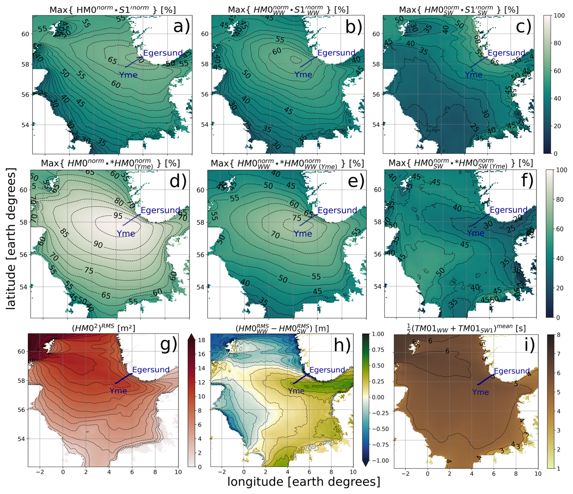
Figure 9Maps of maximum normalized cross-correlation (over the North sea and the full observation period) between the significant wave height components of the wave model and: hourly RMS (a–c), and in situ measurements at Yme (d–f). For the top two rows, the three columns from left to right implement respectively the model: full-spectrum (HM0), wind waves (HM0WW) and swell (HM0SW) significant heights. (g) Total squared RMS of the model significant wave heights. (h) Relative contribution of HM0WW (green) and HM0SW (blue). (i) Model time-averaged center period between swell and wind waves. and correspond to the hourly RMS wind and swell components of (Sect. 4.3).
4.4 Cross-correlation maps
Figure 9 provides an overview of the maximum normalized correlation for the full observation period between a pair of variables in time t and space r. This is calculated as within a symmetric range of ±2 d around the zero-lag time for the standardized variables and , where * denotes cross-correlation, E is the mean or expected value operator in time, and σ denotes the standard deviation. Here, the reference variable x correspond to the wave model significant wave heights at each geographical location over the wider region encompassing the cable for the full-spectrum (Fig. 9a and d), wind waves (Fig. 9b and e) and swell waves (Fig. 9c and f) and y is the corresponding wave component from the: (1) RMS series (Fig. 9a–c), and (2) in situ wave height measurements (Fig. 9d–f).
In the case of (Fig. 9a–c), well-defined maximum normalized correlation distributions in the surroundings of the cable are evident. For instance, for the full-spectrum (Fig. 9a), maximum correlations remain above 65 % over the cable, reaching 70 % close to Egersund. The wind wave component of the model correlates best with in a region of the central North sea close to Yme (Fig. 9b) with maximum correlations surpassing 65 %. This region around Yme, which sustains the overall highest significant wave energy input in proximity to the cable (proportional to the squared RMS of HM0 in Fig. 9g), is also one generally dominated by wind wave over swell contributions (Fig. 9h). The exact location of the region-wide maximum correlation is in fact expected to deviate somewhat from the exact location of Yme due to the generally expected non-flat frequency response of SoP to SGW, noise-related error contributions, and the fact that the maximum correlation region, which is biased towards the NW away from Yme, also corresponds to a regional SGW beam stretching from Shetland to SW Norway with increasing total wind wave energy in that direction (Fig. 9g and h).
The true swell component correlates best with along the SW coast of Norway region around Egersund (Fig. 9c), reaching similar maximum correlations as those for wind waves. This is consistent with the fact that, contrary to Yme, this narrow coastal region, although presenting generally lower wave heights than the open North Sea (Fig. 9g), is dominated by swells (Fig. 9h) and points towards Egersund as the origin location of the swell signal recorded by SoP. Other coastal areas in northern central Europe also tend to accumulate higher correlations likely due to the propagation effect of the non-dispersive, long-wave swells traveling with nearly unchanged waveforms over the relatively shallow North Sea. As the average peak frequency difference between swells and wind waves (Fig. 9i) is largely homogeneous over the cable extent (in the range 0.17–0.2 Hz), the empirical separation frequency used to get and based on the in situ measurements at Yme can be considered a useful approximation for parts of the cable away from Yme, such as Egersund.
Figure 9d–f depict the same type of correlation sets depicted in Fig. 9a–c, although using the in situ measurements at Yme as reference to cross-correlate with the wave model. As expected, the in situ sensors perform better than SoP to estimate full-spectrum and wind wave heights at Yme (Fig. 9a and d and b and e). However, relevant deviations between the reference data occur for the wind wave component (max. correlations below 80 % in Fig. 9e and also confirmed by Fig. D1) and particularly for the swell component (Fig. 9f). The in situ highest correlation distribution of the swells at Yme (Fig. 9f) is marked by a similarity with the regions of overall high swells (Fig. 9h); and the deviations might result from imperfect separation of the swell components from the in situ data and/or the model.
5.1 Swell and wind wave monitoring with SoP
In the previous sections, the capabilities of SoP to detect SGW with a submarine telecommunication cable were studied. Foremostly, it was shown that the parameter can contain detailed signatures related to both (high-frequency) wind waves and (low-frequency) swells that correlate positively with the model and in situ ground truth, reaching maximum correlations of 70 %. The former type of waves dominated the SGW spectrum offshore in the distal part of the cable and consequently wind waves populating the SoP signal are likely to arise from wave activity at Yme, where the cable reaches the water surface and is probably susceptible to wave activity. The latter is evidenced by a spatial correlation map (Fig. 9b) and the decreased wind wave energy near the coast of Egersund (Figs. 8b and 9g and h). The lesser amount of spectral line noise at low frequencies (Fig. 4a) relative to that at higher frequencies is consistent with the higher maximum correlations with the model obtained for swells than for wind waves.
During the observation period, the coastal regions of Norway showed a comparatively more energetic swell signature than the open sea (Fig. 9g and h), such that swell activity observed in the SoP data is probably mostly originated along the SW Norwegian coast in front of Egersund. Future observations on the same cable are prone to provide variable wind-to-swell wave prevalence distributions and energy ratios, as these are prone to fluctuate in the North Sea due to their dependency on large-scale atmospheric circulation variability such as the North Atlantic Oscillation (Semedo et al., 2015). No evidence of tidal modulations was identified in the data, partly due to the location of the cable close to an amphidromic system with minor tides (Sündermann and Pohlmann, 2011).
Based on the observations and the vanishing wave pressure and particle displacements of SGW at depth (Figs. B1 and B2), it is likely that the segments that are more sensitive to sea state variability in the open ocean are located close to the Yme platform, where water depths are less than 100 m and where the backloop segment of the cable rises directly towards the water surface. Direct forced oscillations onto the vertical J-tube hosting the cable at Yme could thus explain the observed SoP signals in the wind wave frequency band, as this tube is likely to have a certain degree of freedom to vibrate and smaller sections of it are semi-suspended in the water.
Contrastingly, even though the swell (and wind) wave activity is in overall larger at Yme than near Egersund (Figs. 8b and c and 9g), it was noticed that the swell component of SoP correlated best with swell activity at the coastal region of Egersund and significantly less so with that at Yme (Fig. 9c). On top of this, the cable is reaching the water surface at Yme while remaining in the seafloor, potentially buried near the coast and the entrance to Nordragabet bay near Egersund. This apparent contradiction suggests differential mechanisms controlling the coupling of wave energy into the cable on either locations. One possible mechanism is the action of shoaling swells in the shallow water coastal area close to Egersund (<50 m, in comparison to water depths of up to 100 m close to Yme, Fig. 2b), which might be capable of triggering significant SoP responses e.g through horizontal flow inducing cable shear or lateral bending and/or dynamic wave pressure loading upon the various kilometers of seafloor cable. At the same time, coastal reflections and shoaling swells might be underestimated by the model near the border of the model domain, where the Egersund coast lies. On the other hand, the surfacing vertical tube hosting the cable at Yme, attached to the subsea tower of the platform appears to respond to (short) wind waves but not as optimal to (long) swell waves. This could suggest that the swell energy, although reaching comparatively larger heights (and perturbation depths) over the extent of vertical cable and the seafloor segments of it close to Yme than at the coast, may be insufficient or inefficient to couple deformation into the fibre, e.g. due to deep burial under sediments in the case of the seabed cable or the sheltering of the cable by the tube in the vertical segment. The wavelength or steepness (height/wavelength ratio) of the waves could potentially play a role in the detection capacity of the vertical segment if e.g. specific mechanical resonance conditions of the vertical tube are met by shorter waves or larger near-surface vertical gradients. These observations require further analyses to be properly elucidated.
The notable difference between the wind wave and swell height components at Yme estimated from the wave model and measured by the in situ ground truth (Fig. D1) highlights the value of having multiple ground truths to measure each of the wave components directly and corroborate model estimates of these. In this case, wave breaking and tentatively wave interactions with the platform seemed to be underestimated by the wave model. At the same time, established methodologies are in place to separate wind and swell spectral components from 1-D time series of surface height variability without the need for additional ground truths (Portilla et al., 2009; Hwang et al., 2012), as is the case of those provided by point sensors or the integrated measurements of SoP. In the latter case this distinction can be significantly more challenging than for point sensors if multiple SGW events with superposed spectral components simultaneously act at various locations along a single cable. However, as mesoscale phenomena such as marine thunderstorms and mesocyclones tend to have scales comparable to the length of the cable (∼120 km), it is normally expected that a single, dominant event at a time will interact with the cable. In the case here explored, the sensitive segments of the cable are confined to at least two distinct shallow cable regions of interest (the ends of the cable), thus keeping the spatial resolution of the measurements shorter than the full cable length. More generally, as the typical separation between repeaters in submarine cables is no larger than about 50 km, rectilinear (straight) cable links typically have such resolutions although this is in fact highly dependent on the geographical extent of shallow water areas covered by the cables such as continental platforms or sediment banks.
Because the spatial correlation of SoP with wind waves and swells is in both cases dominated by regions adjacent to the cable and monotonically decaying outwards, it can be inferred that the forcing is very local and distant ocean microseismic signals are not dominating the signal. However, the influence of local (primary or secondary) microseismic signals (e.g. Cessaro, 1994) cannot be ruled out, as these could potentially influence the SoP signal through seismic surface (Scholte) waves along the seabed generated very close to the cable. For instance, the harmonics observed in the spectrograms during the strongest events (Fig. 4a) could either represent evidence of resonance effects or a secondary microseismic contribution.
Our analysis focused on comparing the SGW-induced pressure with SoP observations. Alternatively, the horizontal or vertical orbital particle displacement of SGW (Eq. B3) could have also been presented here as proxies for induced deformation on the cable, as the oscillatory water motions causing shear stress, shaking or bending of the cable are possible momentum transfer mechanism from the waves into the cable. However, the depth-decay behavior of the former is fairly similar to that of the dynamic pressure already shown in Fig. B1. On the other hand, the vertical particle displacement presents a relatively much faster depth-decay, including the lower frequencies, which are in turn the only capable of interacting with deeper ocean bottoms (Fig. B1).
This work focused on the comparison between SoP measurements and reference data, while the specific physical mechanism(s) (cf. condensation, shearing, torsion, bending) behind the transfer from wave motions into the fibre (see Liu et al., 2025, for a review on the matter) are largely set aside due to the lack of detailed information about the cable and the physical fields distributed along its full span. Compared to phase-recovering FO sensing techniques like DAS, which are predominantly sensitive to axial fibre strain, the stress-induced (radial) birefringence variations that characterize SoP are reportedly nearly omnidirectional (Mecozzi, 2024). Regardless of the fact that the sensitivity of phase-sensitive systems is comparatively higher, this suggests that some of the fibre deformation modes triggered by wave-induced hydrodynamic pressure and flow could potentially result in measurable SoP anomalies that would go unnoticed by the former. More advanced developments such as multiphysics simulations coupled with spatially-resolved reference sensors (ideally in controlled environments) may aid in properly resolving the specific mechanism(s) acting at the seabed to produce the measured anomalies (and their relative contributions).
5.2 Stability of the SoP response
The significant scatter in the bivariate correlation plots between and the reference wave heights (Fig. 7a–d) as well as the anomalously large and sharp peaks of the RMS S1′ (Figs. 4a and b and 8) that do not compare entirely with the relative prominence and shape of the actual wave height variability suggests time-dependent variations in the SoP response and possibly a non-linear component therein (Fig. C1). The largest, breaking wind waves clearly contribute to the observed non-linear trends (Fig. 7c), while swells contribute significantly to the random scatter in the bivariate correlations, suggesting complexities in the swell energy coupling into SoP variations. The generally incoherent accumulation of swell signals (with longer wavelengths than wind waves) over large cable extents could explain the latter behavior.
Previous studies have highlighted the inherently non-linear response of birefringence and incoherent accumulation of SoP changes on fibres (Costa et al., 2023; Mecozzi, 2024). Our SoP data could thus be also influenced by inherent non-linear Stokes vector rotations as a response to external forcing for the particular link under study. On top of this, the approximated Stokes parameter in this work is being analysed without resorting to other Stokes parameters, while the actual variation of each of these as a function of the (multidimensional) Stokes vector rotation in the Poincaré sphere is generally non-linear, as exemplified in Appendix E and Fig. E1. The latter fact also implies that each of the Stokes parameters () is more sensitive to Poincaré sphere rotations when their values are at minimum, i.e. nearly zero (if the Stokes vector is perpendicular to the axis of that particular parameter). Theoretically, in extreme cases the rotation of the Stokes vector could be large enough that transient trajectories in the Poincaré sphere with accumulated rotations of >2π rad could take place, i.e. component wrapping. A detailed analysis of the SoP response here becomes increasingly challenging, reminding ourselves that the instrumental frequency sensitivity of SoP is largely unknown and that the uncalibrated photodiode detectors of the SoP system only provide an estimate of S1 that we have studied in this work.
The causal mechanism(s) explaining the false negative SGW events in SoP lasting hours to several days as e.g. those depicted in Figs. 5 and 6 can only be weakly constrained with the available data due to the lack of in-depth knowledge on the coupling state of the several-km cable and spatially-resolved co-located measurements. A mechanism that could generally explain temporal dips in sensitivity of any of the Stokes parameter to external forcing is related to quasi-stationary (long-term) stabilization of the orientation of the Stokes vector in the Poincaré sphere along parallel planes (in our case small concentric circles along the surface of a sphere, as S0 remains nearly constant) to that defined by the parameter in question. In our case, this would translate into short-term oscillatory forcings only being effectively transferred into the S2,3 components while , even if S1 slowly drifts over time scales larger than SGW variability. Such states are generally unlikely to extend for long periods, as the (three-degrees of freedom) Stokes vector rotations have a marked chaotic nature. A special case of such states happens when the Stokes vector is nearly fixed along S1, where its sensitivity is at minimum (Sect. E). From this it generally follows that systems combining all Stokes vectors are likely to provide a higher degree of stability and linearity in the SoP response as environmental signals that are randomly ill-recovered by some Stokes parameter(s) could be detected more properly by at least another. Despite this, a comparison of the long-term trend of (which was inherently removed for our bandpass analysis on the SGW frequency band) with the aforementioned false negatives provides no clear correspondence as no quasi-static trends match the false negatives (Fig. F1). In particular, the latter events do not match times when was at its maximum, i.e. statistically closest to S1=0 (the actual value of S1 cannot be reliably determined). This suggests other mechanism(s) dominating the observed sensitivity fluctuations of the system.
Although there is a random probability that S1 fluctuations are compensated destructively by the superposition of multiple simultaneous events along different spans of fibre, such net canceling is also only relevant for relatively short timespans and/or short sensitive cable spans owing to the stochastic behavior of the Stokes vector. Thus, this seems unlikely to explain the observed sensitivity lows lasting several-days on such a long cable. A key observation from Sect. 4.2 is that these events predominantly coincide with wind waves at ∼100° heading (Fig. 6, box in Fig. 7b and light blue outliers in Fig. 7c). This strongly suggests a geometrical constraint involved. For instance, a wave shadow from a sheltering body could lead to reduced SGW motions coupling into the cable for waves impinging at certain angle. The adjustable height system of the Yme platform could potentially explain this: as this platform can be heightened by several meters (jack-up type), the tubed cables (these reportedly plunge into the water on one of the sides of the platform) might be fastened to the structure in some way to avoid excessive shaking. In which case, the mechanical state of the cable (e.g. its static tension or stiffness) could be affected and thus its sensitivity. Alternatively, these tubes might simply become more exposed to waves from all directions when the platform is heightened, whereas the structure could block SGW coming from the opposite side if lowered at water level. In contrast, it seems less likely that this apparent directional sensitivity of the cable is determined by the relative orientation between the seafloor cable segment and the SGW directional spectrum, as suggested by their lack of correlation in Fig. 7b. Despite these arguments, the exact causal mechanism for the observed false negatives cannot be determined with confidence due to lack of available data on the mechanical state of the cable and/or platform operation and geometry.
It is also worth noting that, in addition to the aforementioned false negatives, Fig. 7a, c, and d also show the comparatively less dominant presence of a few transient false positive SoP outliers, i.e. high SoP anomalies at times of relatively low waveheights at Yme. From Fig. 5a, the latter are less common than false negatives and cover shorter time spans. These false positives could arise from different noise sources, namely SoP system self-noise, cable perturbations at locations outside of the joint coverage of the wave model and in-situ sensors, including the shallow cable span between the coastline and perturbations in the node room itself. In addition, the superposition of Stokes vector rotations resulting from simultaneous wave events at different cable spans is expected to generally raise the mean SoP variability level. In contrast, such addition of non-deterministic signals with three degrees of freedom seems unlikely to produce mean destructive interference.
As previously suggested, during energetic SGW events, interactions with deeper cable segments could take place if the waves have sufficiently large amplitudes and long wavelengths (Fig. 8), therefore the extent of cable strained by SGW activity is generally a function proportional to the wave height and period. The exact length of perturbed cable is currently challenging to estimate because the exact transfer function from SGW pressure-to-SoP (or water flow-to-SoP) anomaly is not known. This further increases the probability that the SGW response of SoP deviates from a linear one, as rougher sea states and SGW variability with wider spatial extents tend to affect larger cable segments simultaneously. This could explain the increased amount of random scatter in the bivariate correlations for swells relative to those of the wind waves (Fig. 9d and c, respectively), as the former contains simultaneous contributions at separate cable segments (Fig. 8c) from the same trains of swell waves (Fig. 9c and i). In terms of absolute SGW-induced pressure, the deeper part of the vertical cable segment at Yme experiences, on average, dynamic pressures between 1 and 10 kPa (Fig. 8). At the water surface, the maximum excess pressure approaches 100 kPa. For context, 10 kPa is the differential pressure exerted by a SGW of ∼1 m in amplitude at the mean water surface, while 10 mPa is the RMS acoustic pressure at the lower end of the dominant ambient underwater noise in the range 63–500 Hz along the Scottish North-Sea coast (equivalent to a sound pressure level at 80 dB re 1 µPa2, Merchant et al., 2016). Notice that the scaling value from to wave height found in Sect. 4.2 effectively represents a first-order estimate of the mean sensitivity of this parameter to SGW heights (in the 0.03–06 Hz band) for the SoP sensor and cable link combination here considered (weighted by the specific cable spans that are most sensitive) and it should be empirically verified by other experiments.
At the current state, the implemented SoP system suffers from non-negligible noise contributions that can intermittently obscure weaker SGW signals and prompts future improvements in its internal design and the acquisition set-up. The main ones being: (1) a modulated line spectrum dominant above 0.2 Hz likely related to the SoP transmitter noise at selective frequencies spread over a wide band but in this case primarily affecting peak frequency estimation (Fig. 5b) and high-frequency wave heights, i.e. wind waves and short-period swells (Figs. 4a and 5b), and (2) EDFA noise, whose noise spectrum tends to be wide-band. This limitation could be addressed by means of further refinement of the SoP system such as more stable laser sources with improved noise characteristics. Secondary noise sources close to any segment(s) of the several-kilometer link, such as those exposed to anthropogenic activity, infrastructure-related noise or active equipment at the node rooms at both Yme and Egersund (vibrational, EM and/or thermal noise from e.g. server racks, human activity or air conditioning systems or pulling or sudden impacts on the cable at the platform site during offshore operations) are also capable of interfering to variable extents with the SGW measurements and producing outliers. A careful pre-survey of potential noise sources seems key to properly interpret SoP data. Although most of the aforementioned noise sources typically exist at frequencies outside the SGW band and are expected to have a rather transient character, these could temporarily obscure the ocean wave signals in short time windows if overlapping spectrally with the SGW frequency band. At the same time, the frequency response of SoP is not necessarily flat, meaning that some spectral bands might be affected by noise more than others.
5.3 Operational considerations for SoP measurements
One of the main drawbacks of SoP is that its spatial resolution is restricted by the length of the entire FO link under analysis, i.e. the measured signal is an accumulate of the net variability acting along the entire sensed fibre. This makes SoP implementations more attractive for shorter links regions with spatially uniform variability to avoid interpretation ambiguities that could arise if multiple SGW events overlap in time at different cable parts, especially in shallower water regions with high SGW spatial variability. Alternative fibre looping architectures in repeatered cables can improve the spatial resolution up to the separation between repeaters with high-loss loop backs (Marra et al., 2022; Yaman et al., 2025). In contrast, distributed FO sensing techniques are single-ended i.e. these only require one fibre end to operate, have selectable spatial resolutions (up to meters of fibre), EM noise resistance and higher measurand sensitivities. For instance, a method like DAS is capable of constraining and linearly quantifying the specific sensitivity spots that capture SGW variability and could thus provide estimates of the strain induced by SGWs on the cable. Underwater surveys of the cable would also provide further details that would help better constrain its structural and geometrical setting, which are pivotal to accurately explain the detection capacity of the cable.
On the other hand, SoP is a more cost-effective, scalable and simpler to design technique in comparison to other fibre-optic sensing techniques that does not require bulky, costly, maintenance-demanding or highly-specialized measuring components. In fact, most optical telecommunication systems currently use SoP as a modulation technique along with amplitude, frequency and phase modulation schemes. This implies that SoP information is currently being continuously decoded in subsea cables around the world (at rates ranging between 0.01 to 1.6 Tb s−1). However, this high-rate data is rarely stored by most vendors and user access to private-owned cables can be costly or restricted. Furthermore, modern network management channels only support bit rates of much less than a few kb s−1, meaning that dedicated SoP detectors must be used in order to harness this information. Therefore, modern optical telecommunication networks still require some software as well as hardware modifications in order to allow for continuous SoP monitoring without sensor attachments. However, we highlight the possibility to achieve this through common effort from cable providers and users, especially if enough interest stems on FO sensing on behalf of governments, stakeholders and other potential users of the ocean science and technology community. The same effort is likely to render commercial FO cables more accessible for the ocean community in terms of data and service availability as well as usage fees.
While shorter fibre links reduce spatial ambiguity for SoP and thus generally increase the chance of correct interpretations, its compatibility with subsea cable repeaters allows sensing ranges of more than 10 000 km along existing trans-oceanic fibre-optic infrastructure. Such large coverage capabilities could be useful for links exhibiting SGW anomaly distributions well-constrained in space, for the detection of very large scale ocean waves with wavelengths comparable to or larger than the links, e.g. tsunamis or tides, and for large mesoscale to synoptic scale studies. In contrast, most DAS units usually cover less than 200 km. The technology has recently been demonstrated to reach more than 2200 km at sampling rates of nearly 1.8 kHz (Rønnekleiv et al., 2025) with subsea cables, the usable range decreasing proportional to sampling rate and with the requirement of repeaters with special amplification and circulation assemblies which are not typically incorporated in modern telecommunication networks. A more recent work (Mazur et al., 2025) has nearly tripled the former coverage range with an alternative approach that is compatible with modern commercial transoceanic cable architectures.
SoP experiments on different cables and covering a few years would be valuable to confirm the stability of the SoP transfer function over time for a particular link, especially since SoP exhibits a non-stationary behavior (Pellegrini et al., 2025), i.e. quasi-static variations in the thermal or mechanical state of any cable segment (as e.g. at the Yme platform) that sporadically re-adjust the SoP. Ambient temperature variations are known to temporarily degrade the SNR of SoP (Marra et al., 2022). This adds up to the naturally occurring fluctuations in the initial polarization state injected into the fibre for conventional laser sources, e.g. due to thermal oscillations at or around the transmitter. The latter could be addressed by careful selection of transmitter components as well as monitoring and active control of temperature in acquisition rooms. The characterization and isolation of machines and other devices potentially generating non-negligible thermal, EM and/or vibrational noise close to the acquisition area is strongly encouraged. We further emphasize that SoP values are dynamic (as opposed to absolute, static measurements), relative-valued and only represent first-order estimates of the true SGW variability at one location.
A more general limitation of SoP, also confronted by well-established oceanographic SGW sensors is the necessity to have the sensing element in situ or close enough to the water surface due to the vanishing SGW dynamic pressure and orbital displacement in proportion to depth and wave frequency. For SGW monitoring, this might limit the usage of deep and/or buried subsea telecommunication cables segments while bringing reliance towards very shallow (e.g. estuarine or coastal) or surfacing ones. Alternatively, dedicated installations of light-weight cables could circumvent the dependence on telecommunication cables of no practical use, having in mind that a single cable hosting several fibres (and optionally power lines) is compatible with multiple FO sensing techniques as well as being useful for data transfer and communication with other sensors. An additional, current challenge is to filter-out optical frequency-dependent self-noise from the implemented system as this could contribute to smear out the true gravity wave signatures. However, improvements in the optical components of the SoP device (e.g. transmitter and ADC) are achievable and could readily produce a cleaner signal with a wider-band frequency response, thus providing more accurate approximations of the sea state variability.
Nearly 8 % of the ocean surface is at depths below 200 m (i.e. continental shelves and coasts, Paris et al., 2016) while about 16 % of the subsea cables cross such depths (nearly 30 % down to 1500 m, Clare et al., 2023). This implies that a non-negligible portion of the extensive and robust network of existing telecommunication cables around the world has the potential to be implemented for SGW monitoring with FO techniques. Deeper cables (below ∼2 km) are generally restricted to the detection of long waves such as tides, tsunami or low-frequency infra-gravity waves. The remotely-operated SoP devices allow for straight-forward data management, enhanced real-time capabilities, and significant data loss resilience, as no battery support for the sensing elements (i.e. the fibres) or data recovery campaigns are required. Applications that could benefit from SoP systems include early-warning systems, infrastructure monitoring and sea-state information platforms. SoP sensing appears particularly promising for time-resolved, continuous real-time monitoring of specific wave events (e.g. extreme waves or tsunamis) in difficult-to-access regions where limited or no other (temporal or permanent) oceanographic sensors might be available or in locations of high interest (e.g. for marine energy harnessing and other offshore installations). This could prove valuable to monitor and protect offshore as well as coastal infrastructure.
Our results demonstrate that surface gravity wave variability can be continuously monitored over several months with conventional subsea telecommunication cables and State of Polarization (SoP) sensing devices. Detailed spectral characteristics of the sea surface variability can be remotely recovered at high sampling rates and it is possible to detect both wind waves and swells in the range 0.03–0.6 Hz acting simultaneously on different segments of the interrogated cable through a single, 1D measurement. The potential separation of these spectral and spatial components without additional ground truths prompts further investigation and future improvements in the noise characteristics of the SoP device. Previous studies showed the capacity of SoP to detect SGW, here we quantitatively advanced this knowledge through a detailed comparison of SoP data with in situ and model ground truths. Specifically, we find positive correlations of nearly 70 % between the hourly RMS Stokes parameter and the true full-spectrum significant wave heights. SGW peak frequency estimation from SoP is also possible but was significantly affected by instrumental noise of the here implemented device. We present evidence that the (high-frequency) wind wave variability component contributing to the SoP signal is mainly originated at open sea close to the Yme site, while the dominant (low-frequency) swell wave signature is likely of near-coastal origin. This is foremostly due to the uneven spatial energy partition of these wave components between both regions and potentially also due to the energy coupling of the two SGW components onto cable segments having variable (primarily over space and secondarily over time) depth, burial, geometrical and mechanical conditions. Furthermore, we observe that the SGW detection capacity of SoP is not azimuthally uniform, tentatively in relationship with the geometrical interaction of the wavefield with infrastructure supporting the cable. The signals retrieved from SoP sensing are currently non-dimensional quantities and should only be considered as dynamic, first-order estimates of the variability of SGW.
Aside from these current limitations, SoP sensing can also be considered a relatively simple-to-build and scalable solution to monitor a proxy for sea state variability remotely and in real-time where cables are in sufficient proximity to the water surface in comparison to the wavelength of interest. A non-negligible portion of the existing network of subsea telecommunication cables has the potential to be turned into a network of sensors of opportunity in key ocean regions worldwide. Applications that could tentatively benefit from such infrastructure include: sea-state monitoring, early warning systems, coastal and offshore facility protection, and oceanographic modeling.
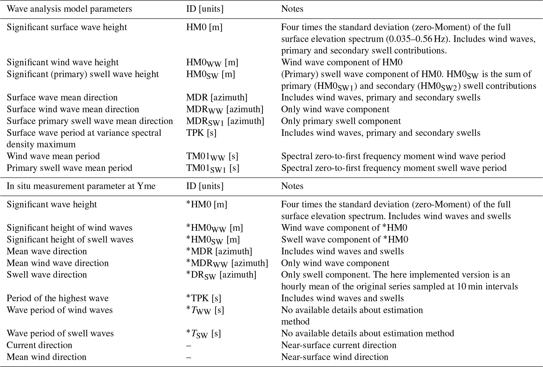
Table A1Wave analysis model and in situ point measurement parameters considered (at Yme) in this work. The namings and identifiers (IDs) of the model parameters are as reported in the model metadata. The same applies for the naming of the parameters derived from the in situ sensors at Yme, whose ID (marked with asterisks, e.g. *ID) has been introduced in this work in analogy to the model IDs. Each sample of the wave model parameters is an average over an area of ∼11 km2. Further details about the calculation of the specific modeled variables can be found in ECMWF (2024).
To obtain an estimate of pSGW, the magnitude of the dynamic pressure induced by a SGW of amplitude a, frequency f at a certain depth over water with maximum depth h, we use the linear SGW depth-attenuation relation (e.g. Massel, 2017):
where g is the average gravity acceleration at the location of interest and ρ is a representative water density. The wavenumber (λ being the SGW wavelength) can be obtained by solving the linear SGW dispersion relation numerically:
where and T is the period of the SGW. The magnitude of the horizontal (uSGW) and vertical (wSGW) orbital water particle displacements induced by SGW are estimated as:
Using Eqs. (B1) and (B3), one can estimate the depth-frequency distribution for SGW dynamic pressure, horizontal and vertical particle motions for a given total water column height (Fig. B1). The decay of pressure and horizontal displacement is fairly similar, except that horizontal motions at frequencies below about 0.04 Hz remain nearly unattenuated at the mean depth of the central North Sea banks (100 m), the region where Yme platform is fixed. Vertical motions generally decay comparatively more rapidly at depth.
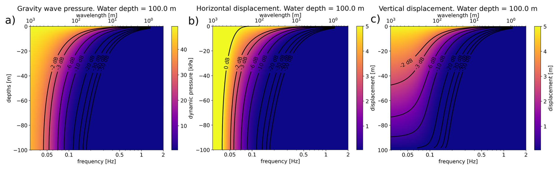
Figure B1Depth-frequency distribution of linear surface gravity wave pressure (a), horizontal (b) and vertical (c) orbital displacement at 100 m-depth water for a 10 m-height sinusoidal wave (roughly the depths at Yme and the maximum observed significant wave height, respectively). Contour values in dB relative to surface values.
Using Eqs. (B1) and (B2), one can also estimate how SGW with particular frequencies interact with the bottom and decay as a function of water depth for a fixed SGW amplitude, as shown in Fig. B2 for the subsea cable layout. SGW below 0.05 Hz are attenuated by a factor of 10 at water depths of 250 m for total water column heights of more than 300 m (Fig. B2a). On the other hand, SGW at frequencies of 0.1 Hz decay by 10 dB at water depths of 60 m for seabed depths beyond about 100 m, while those above 0.2 Hz are in most cases unaffected by the seafloor depth and generally only reach a few tens of meters below the water surface or less.
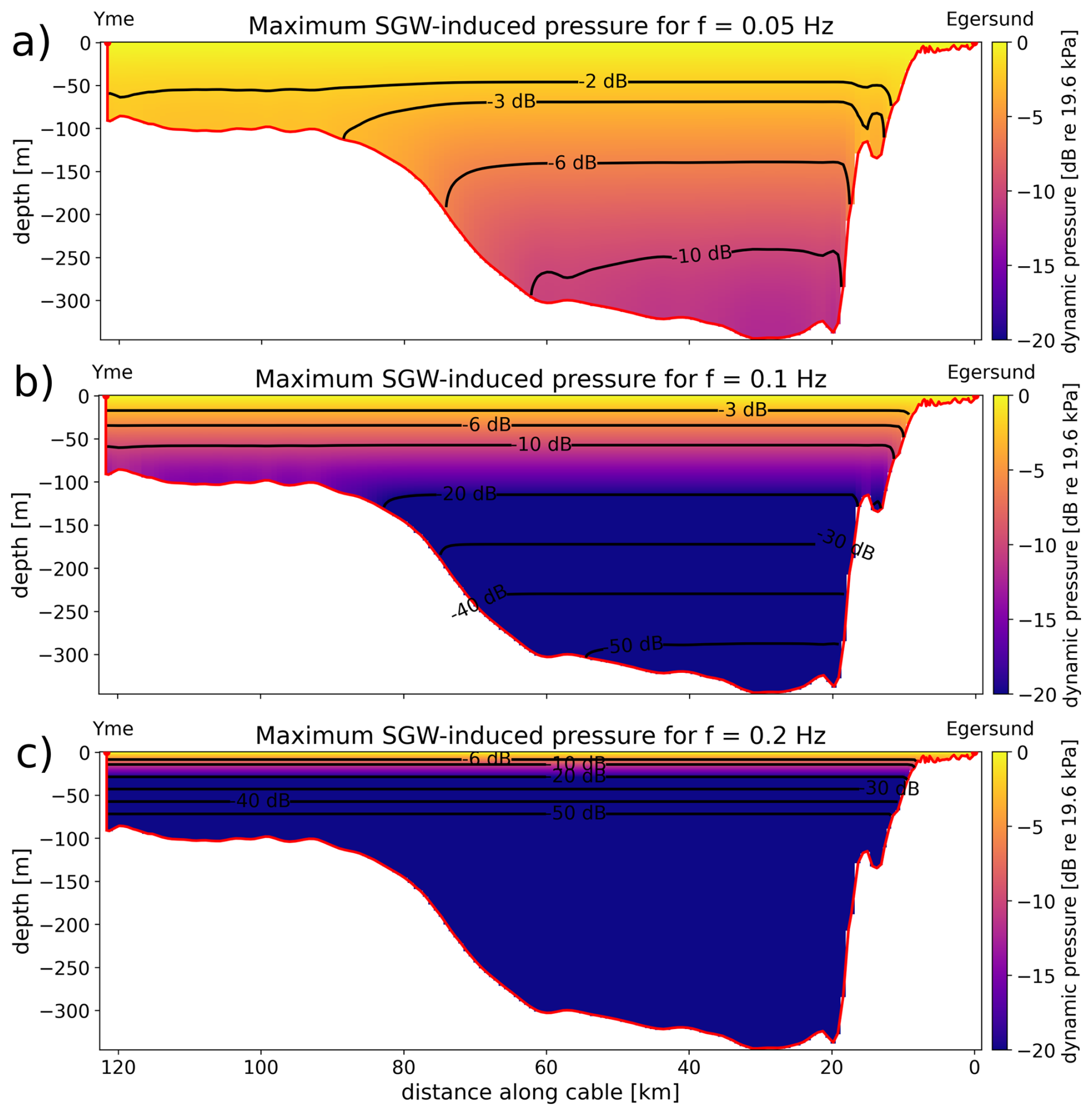
Figure B2Linear surface gravity wave pressure amplitude depth distribution along the cable bathymetry profile for three different frequencies: (a) 0.05 Hz, (b) 0.1 Hz, (c) 0.2 Hz. Contours and colormap in dB relative to the (maximum) pressure value induced by a SGW of 2 m height at the water surface on each case.
Figure C1 depicts the linear regression statistics of Fig. 7a, including a normalized residual plot (Fig. C1a) that evidence relatively large regression residuals and a slightly biased distribution of these towards high values of the hourly RMS. A quantile-quantile plot shows a mostly linear correlation for the majority of the data values, except for the upper quantiles, which reflect a clear non-linear component likely related to steep wave effects such as wave breaking (Fig. C1b).
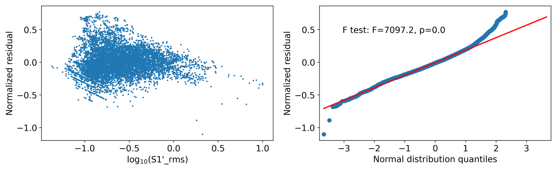
Figure D1 shows the degree of correlation between the wave analysis model and the in situ SGW height and direction measurements from a buoy and a radar at the Yme location. HM0 shows good consistency at this site between the model and the in situ measurements (Fig. D1a), while on the other hand, the wind (HM0WW) and swell (HM0SW(1)) components (Fig. D1b and c) present significant deviations that can relate to: (1) the wave spectrum partitioning technique of both data types, as well as the 2D spatially-averaged wave model vs. the (1D) in situ point sensor measurements, and/or (2) dynamic wave effects such as breaking, wind-interactions, or flow effects potentially not properly accounted for in the model. The difference is more significant for swells, where the points with largest errors coincide with those having the largest deviations in estimated dominant wave direction (Fig. D1c) and evidences that the model tends to underestimate the swell heights considerably.
In the case of wind waves (Fig. D1b), the red dots connecting each dot having in situ wave heights above 3 m represent the regular wave breaking limit Hb calculated from the wave steepness as (Massel, 2017) and found using the approximate explicit solution of Eq. (B2) for k as (Guo, 2002) and the in situ wind wave period (*TWW) at each time step. The water depth h at Yme is set to 90 m. This shows how most measured waves above about 3 m are either just above or approaching the theoretical wave breaking limit, which seems to be disregarded by the model and explains the cut-off leveling of in situ wave between 5–6 m.
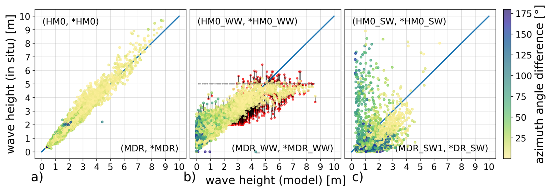
Figure D1Bivariate correlation plot between the significant wave height reference data from the wave model (x axis) and the in situ data at Yme (variables indicated in the upper left part of each panel) for: (a) full-spectrum surface height, (b) wind waves (red dots are the theoretical wave breaking height for each measurement and the dashed black line marks an estimated wave breaking height limit at 5 m), and (c) swells. The color scale represents the difference between the wave direction parameters indicated in the lower right of each panel.
Assuming that a Stokes vector rotation along a great circle of the Poincaré sphere, containing the axis of one of the Stokes parameters, e.g. S1, then from 1 we can formulate S1=S0cos (θ) for a given Stokes rotation angle θ (relative to the S1 axis in the Poincaré domain). The net variation of S1 as a function of θ can then expressed as: . This sensitivity towards θ is illustrated in Fig. E1.
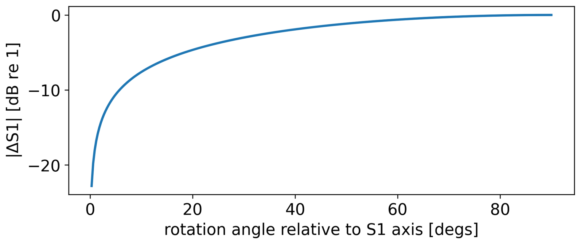
Figure E1The sensitivity of a single Stokes parameter (or any linear combination of these) to a rotation of the Stokes vector in the Poincaré sphere along a great circle described by the parameter axis.
An alternative way to reach the same result is combining the definition of S1 (Eq. 1b) and the (randomly oriented) components of a plane-polarized EM wave with electric field amplitude E propagating along the fibre axis (z axis) as , where α is the physical angle between the x axis and the oscillation plane of the wave:
The sensitivity of S1 to variations in α will be maximum when the rate of change of is maximized, i.e. if . This corresponds to the oscillation plane of the EM wave at 45° from the x and y axes and thus S1=0. Conversely, the rate of change becomes zero when the oscillation plane is aligned with x or y, i.e. when is at maximum value.
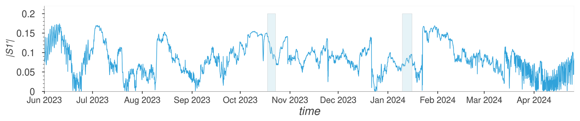
Data available from Pelaez Quiñones et al. (2026), https://doi.org/10.17605/OSF.IO/Q5E2N.
JPQ conceptualized the study, processed and analyzed the data, and prepared the manuscript. SB conceptualized the study and provided the SoP data. All authors contributed to the interpretation of the results and reviewed the manuscript.
The contact author has declared that none of the authors has any competing interests.
Publisher's note: Copernicus Publications remains neutral with regard to jurisdictional claims made in the text, published maps, institutional affiliations, or any other geographical representation in this paper. The authors bear the ultimate responsibility for providing appropriate place names. Views expressed in the text are those of the authors and do not necessarily reflect the views of the publisher.
This research has been supported by the Universitetet i Bergen, Matematisk-Naturvitenskapelige Fakultet, Universitetet i Bergen (SFI Smart Ocean (Norwegian Research Council), grant no. 309612).
This paper was edited by Anne Marie Treguier and reviewed by two anonymous referees.
Ardhuin, F., Rogers, E., Babanin, A. V., Filipot, J.-F., Magne, R., Roland, A., van der Westhuysen, A., Queffeulou, P., Lefevre, J.-M., Aouf, L., and Collard, F.: Semiempirical Dissipation Source Functions for Ocean Waves. Part I: Definition, Calibration, and Validation, J. Phys. Oceanogr., 40, 1917–1941, https://doi.org/10.1175/2010JPO4324.1, 2010. a, b
Barcik, P. and Munster, P.: Measurement of slow and fast polarization transients on a fiber-optic testbed, Opt. Express, 28, 15250–15257, https://doi.org/10.1364/OE.390649, 2020. a
Bjørnstad, S., Yamase Skarvang, K. S., Roar Hjelme, D., Tunheim, A., Fjermestad, F., and Østerli, E.: First Impact Movement Characterization of Shallow Buried Live Subsea-Cable, in: 2024 Optical Fiber Communications Conference and Exhibition (OFC), 1–3, https://doi.org/10.1364/OFC.2024.M4E.4, 2024. a, b
Bruciaferri, D., Tonani, M., Lewis, H. W., Siddorn, J. R., Saulter, A., Castillo Sanchez, J. M., Valiente, N. G., Conley, D., Sykes, P., Ascione, I., and McConnell, N.: The Impact of Ocean-Wave Coupling on the Upper Ocean Circulation During Storm Events, J. Geophys. Res.-Oceans, 126, e2021JC017343, https://doi.org/10.1029/2021JC017343, 2021. a, b, c
Carver, C. J. and Zhou, X.: Polarization sensing of network health and seismic activity over a live terrestrial fiber-optic cable, Commun. Eng., 3, https://doi.org/10.1038/s44172-024-00237-w, 2024. a
Cessaro, R. K.: Sources of primary and secondary microseisms, B. Seismol. Soc. Am., 84, 142–148, https://doi.org/10.1785/BSSA0840010142, 1994. a
Chang, E. K.-M.: CMIP5 Projected Change in Northern Hemisphere Winter Cyclones with Associated Extreme Winds, J. Climate, 31, 6527–6542, https://doi.org/10.1175/JCLI-D-17-0899.1, 2018. a
Charlton, D., Clarke, S., Doucet, D., O'Sullivan, M., Peterson, D., Wilson, D., Wellbrock, G., and Bélanger, M.: Field measurements of SOP transients in OPGW, with time and location correlation to lightning strikes, Opt. Express, 25, 9689–9696, https://doi.org/10.1364/OE.25.009689, 2017. a
Clare, M., Lichtschlag, A., Paradis, S., and Barlow, N. L. M.: Assessing the impact of the global subsea telecommunications network on sedimentary organic carbon stocks, Nat. Commun., 14, https://doi.org/10.1038/s41467-023-37854-6, 2023. a
Colosi, L., Pizzo, N., Grare, L., Statom, N., and Lenain, L.: Observations of Surface Gravity Wave Spectra from Moving Platforms, J. Atmos. Ocean. Tech., 40, 1153–1169, https://doi.org/10.1175/JTECH-D-23-0022.1, 2023. a
Costa, L., Varughese, S., Mertz, P., Kamalov, V., and Zhan, Z.: Localization of seismic waves with submarine fiber optics using polarization-only measurements, Commun. Eng., 2, https://doi.org/10.1038/s44172-023-00138-4, 2023. a, b
Dejdar, P., Myska, V., Munster, P., and Burget, R.: Trains Detection Using State of Polarization Changes Measurement and Convolutional Neural Networks, in: 2021 IEEE International Symposium on Inertial Sensors and Systems (INERTIAL), 1–4, https://doi.org/10.1109/INERTIAL51137.2021.9430469, 2021. a
ECMWF: IFS Documentation CY49R1 – Part VII: ECMWF Wave Model, Chap. 7, European Centre for Medium-Range Weather Forecasts, https://doi.org/10.21957/8315ddc858, 2024. a
Fang, Z., Chin, K. K., Cai, H., and Qu, R.: Fundamentals of Optical Fiber Sensors, John Wiley & Sons, Ltd, https://doi.org/10.1002/9781118381717, 2012. a, b
Ferretti, G., Zunino, A., Scafidi, D., Barani, S., and Spallarossa, D.: On microseisms recorded near the Ligurian coast (Italy) and their relationship with sea wave height, Geophys. J. Int., 194, 524–533, https://doi.org/10.1093/gji/ggt114, 2013. a
Guo, J.: Simple and explicit solution of wave dispersion equation, Coast. Eng., 45, 71–74, https://doi.org/10.1016/S0378-3839(02)00039-X, 2002. a
Hartog, A.: An Introduction to Distributed Optical Fibre Sensors, CRC Press, Boca Raton, FL, US, https://doi.org/10.1201/9781315119014, 2017. a, b
Hwang, P. A., Ocampo-Torres, F. J., and García-Nava, H.: Wind Sea and Swell Separation of 1D Wave Spectrum by a Spectrum Integration Method, J. Atmos. Ocean. Tech., 29, 116–128, https://doi.org/10.1175/JTECH-D-11-00075.1, 2012. a, b
Kossin, J., Emanuel, K., and Vecchi, G.: The poleward migration of the location of tropical cyclone maximum intensity, Nature, 509, 349–352, https://doi.org/10.1038/nature13278, 2014. a
Kossin, J., Knapp, K., Olander, T., and Velden, C.: Global increase in major tropical cyclone exceedance probability over the past four decades, P. Natl. Acad. Sci. USA, 117, 11975–11980, https://doi.org/10.1073/pnas.1920849117, 2020. a
Lionello, P., Günther, H., and Janssen, P. A. E. M.: Assimilation of altimeter data in a global third-generation wave model, J. Geophys. Res.-Oceans, 97, 14453–14474, https://doi.org/10.1029/92JC01055, 1992. a
Liu, M., Costa, L., Mertz, P., Varughese, S., Edirisinghe, S., Kamalov, V., and Zhan, Z.: Trans-Oceanic Distributed Sensing of Tides Over Telecommunication Cable Between Portugal and Brazil, Geophys. Res. Lett., 52, e2024GL114414, https://doi.org/10.1029/2024GL114414, 2025. a
Mann, M., Rahmstorf, S., Kornhuber, K., Steinman, B. A., Miller, S. K., and Coumou, D.: Influence of Anthropogenic Climate Change on Planetary Wave Resonance and Extreme Weather Events, Sci. Rep.-UK, 7, 45242, https://doi.org/10.1038/srep45242, 2017. a
Marra, G., Fairweather, D. M., Kamalov, V., Gaynor, P., Cantono, M., Mulholland, S., Baptie, B., Castellanos, J. C., Vagenas, G., Gaudron, J.-O., Kronjäger, J., Hill, I. R., Schioppo, M., Edreira, I. B., Burrows, K. A., Clivati, C., Calonico, D., and Curtis, A.: Optical interferometry–based array of seafloor environmental sensors using a transoceanic submarine cable, Science, 376, 874–879, https://doi.org/10.1126/science.abo1939, 2022. a, b, c
Massel, S. R.: Ocean Surface Waves: Their Physics And Prediction, Chap. 4, Advanced Series On Ocean Engineering, 3rd edn., World Scientific Publishing Co Pte Ltd, ISBN: 9789813228375, 2017. a, b, c
Mazur, M., Fontaine, N. K., Karrenbach, M., Ryf, R., Dallachiesa, L., Winter, D., Kamalov, V., Naik, J., Padmaraju, K., Mistry, A., Chen, H., and Neilson, D. T.: High Resolution Distributed Fiber-Optic Sensing Over Repeated Trans-Oceanic Cables, in: 2025 30th OptoElectronics and Communications Conference (OECC) and 2025 International Conference on Photonics in Switching and Computing (PSC), 1–4, https://doi.org/10.23919/OECC/PSC62146.2025.11110694, 2025. a
Mecozzi, A.: Sensing with submarine optical cables, APL Photonics, 9, 070902, https://doi.org/10.1063/5.0210825, 2024. a, b, c, d
Mecozzi, A., Cantono, M., Castellanos, J. C., Kamalov, V., Muller, R., and Zhan, Z.: Polarization sensing using submarine optical cables, Optica, 8, 788–795, https://doi.org/10.1364/OPTICA.424307, 2021. a, b, c, d
Merchant, N. D., Brookes, K. L., Faulkner, R. C., Bicknell, A. W. J., Godley, B. J., and Witt, M. J.: Underwater noise levels in UK waters, Sci. Rep.-UK, 6, https://doi.org/10.1038/srep36942, 2016. a
Namihira, Y., Horiuchi, Y., Ryu, S., Mochizuki, K., and Wakabayashi, H.: Dynamic polarization fluctuation characteristics of optical fiber submarine cables under various environmental conditions, J. Lightwave Technol., 6, 728–738, https://doi.org/10.1109/50.4059, 1988. a
Paris, P. J., Walsh, J. P., and Corbett, D. R.: Where the continent ends, Geophys. Res. Lett., 43, 208–212, https://doi.org/10.1002/2016GL071130, 2016. a
Pelaez Quiñones, J., Bjornstad, S., Thomas, P. J., and Lunde, P.: State of Polarization on Egersund-Yme subsea cable, June 2023–April 2024, OSF [data set], https://doi.org/10.17605/OSF.IO/Q5E2N, 2026. a
Pellegrini, S., Minelli, L., Andrenacci, L., Rizzelli, G., Pilori, D., Bosco, G., Della Chiesa, L., Crognale, C., Piciaccia, S., and Gaudino, R.: Overview on the state of polarization sensing: application scenarios and anomaly detection algorithms, J. Opt. Commun. Netw., 17, A196–A209, https://doi.org/10.1364/JOCN.537881, 2025. a, b
Portilla, J., Ocampo-Torres, F. J., and Monbaliu, J.: Spectral Partitioning and Identification of Wind Sea and Swell, J. Atmos. Ocean. Tech., 26, 107–122, https://doi.org/10.1175/2008JTECHO609.1, 2009. a
Rønnekleiv, E., Sørgård, T., Klimentov, D., Tolstik, N., Waagaard, O. H., Jacobsen, J., Stabo-Eeg, F., Sab, O. A., Calsat, A., Plantady, P., and Brenne, J. K.: Range-scalable distributed acoustic sensing with EDFA repeaters demonstrated over 2227 km, Opt. Lett., 50, 25–28, https://doi.org/10.1364/OL.542267, 2025. a
Semedo, A., Vettor, R., Øyvind Breivik, Sterl, A., Reistad, M., Soares, C. G., and Lima, D.: The wind sea and swell waves climate in the Nordic seas, Ocean Dynam., 65, 223–240, https://doi.org/10.1007/s10236-014-0788-4, 2015. a
Skarvang, K. S. Y., Bjørnstad, S., and Hjelme, D. R.: A Practical Approach to Vibration Monitoring on a Metro Length Fiber Cable Using Low-Cost State of Polarization Monitoring, in: 2023 IEEE Photonics Society Summer Topicals Meeting Series (SUM), 1–2, https://doi.org/10.1109/SUM57928.2023.10224456, 2023. a
Sündermann, J. and Pohlmann, T.: A brief analysis of North Sea physics, Oceanologia, 53, 663–689, https://doi.org/10.5697/oc.53-3.663, 2011. a, b
Wei, J., Gong, W., Xing, J., and Xu, H.: Distributed acoustic sensing technology in marine geosciences, Intell. Mar. Technol. Syst., 2, 71–74, https://doi.org/10.1007/s44295-024-00039-y, 2024. a
Wuttke, J., Krummrich, P. M., and Rosch, J.: Polarization oscillations in aerial fiber caused by wind and powerline current, IEEE Photonic. Tech. L., 15, 882–884, https://doi.org/10.1109/LPT.2003.811143, 2003. a
Yaman, F., D'Amico, A., Han, S., Fujisawa, S., Mateo, E., and Inoue, T.: Span-Based Polarization Sensing in Cables Without Reflectors, in: 2025 30th OptoElectronics and Communications Conference (OECC) and 2025 International Conference on Photonics in Switching and Computing (PSC), 1–4, https://doi.org/10.23919/OECC/PSC62146.2025.11110744, 2025. a, b
Yin, S.: Distributed Fiber Optic Sensors, in: Fiber Optic Sensors, edited by: Yu, F. T. S. and Yin, S., Marcel Dekker Inc. New York, Basel, 183–234, https://doi.org/10.1201/9781420053661, 2002. a
Zhan, Z., Cantono, M., Kamalov, V., Mecozzi, A., Müller, R., Yin, S., and Castellanos, J. C.: Optical polarization–based seismic and water wave sensing on transoceanic cables, Science, 371, 931–936, https://doi.org/10.1126/science.abe6648, 2021. a, b, c
- Abstract
- Introduction
- Theoretical background
- Experimental set-up and data sources
- Observations
- Discussion
- Conclusions
- Appendix A: Summary of parameters and acronyms
- Appendix B: Linear surface gravity wave calculations
- Appendix C: Regression statistics
- Appendix D: Comparison of ground truth significant wave height components at Yme
- Appendix E: The sensitivity of a Stokes parameter to great circle rotation
- Appendix F: Long-term trend of SoP
- Data availability
- Author contributions
- Competing interests
- Disclaimer
- Financial support
- Review statement
- References
- Abstract
- Introduction
- Theoretical background
- Experimental set-up and data sources
- Observations
- Discussion
- Conclusions
- Appendix A: Summary of parameters and acronyms
- Appendix B: Linear surface gravity wave calculations
- Appendix C: Regression statistics
- Appendix D: Comparison of ground truth significant wave height components at Yme
- Appendix E: The sensitivity of a Stokes parameter to great circle rotation
- Appendix F: Long-term trend of SoP
- Data availability
- Author contributions
- Competing interests
- Disclaimer
- Financial support
- Review statement
- References