Internal tides–cyclonic eddy interaction and intermodal energy pathways: evidence from 3 km NEMO-AMAZON36 simulations

The interaction between internal tides (ITs) and mesoscale features plays a key role in ocean energy dissipation. Understanding how IT energy is transformed in energetic western boundary regions remains a central challenge, particularly in regions of vigorous mesoscale activity.

To this aim, we apply vertical mode decompositions to the high-resolution (3 km) simulations during September–December 2015. This study shows that the IT vertical mode and the precise point of IT-eddy encounter determine whether the IT energy propagates freely, deviates, or is trapped, and how topography and coherent eddies synergistically scatter energy between baroclinic modes off the Amazon shelf.

Three representative interaction cases, each captured in a separated 25 h snapshot, were examined: undisturbed propagation until crossing the Ceará Rise seamount, interaction with a cyclonic eddy (CE) core, and interaction with a CE eastern edge. The principal findings establish two points.

First, an IT response (propagation, deviation or scattering) is dually controlled by its vertical mode, and the mesoscale encounter location along with the associated background conditions (currents and stratification). In the absence of a strong eddy, the Mode-1 IT propagates as a coherent beam with a long propagation range (O(1100 km)). In the presence of a strong CE, however, the IT beams are disrupted, preventing sustained long-range transmission. Within the eddy core, the Mode-1 IT is coherently refracted northward (∼ 35° relative to its northeastward incident direction) while maintaining high energy fluxes exceeding 200 W m⁻¹. At the CE edge, Mode-1 is diffracted into two distinct branches, with one propagating northward (∼ 39°) and the other eastward (∼ 35°). In contrast, the IT higher modes are highly susceptible to blocking and trapping: Mode-2 energy, despite initial amplitudes comparable to Mode-1, is strongly blocked at the CE-seamount interface, while Mode-3 remains weak (below 200 W m⁻¹) and less propagative.

Second, intermodal energy transfer is governed by a hierarchical synergy between the seamount and CE's background flow. In the absence of an eddy, the seamount drives a forward energy cascade ($O\left({\mathrm{10}}^{-\mathrm{8}}\mathrm{W}\mathrm{m}{\mathrm{kg}}^{-\mathrm{1}}\right)$) from the Mode-1 IT to higher modes. In contrast, in the presence of a CE, the CE's strong horizontal shear triggers a competing inverse energy cascade ($O\left({\mathrm{10}}^{-\mathrm{8}}\mathrm{W}\mathrm{m}{\mathrm{kg}}^{-\mathrm{1}}\right)$) from the background flow to the IT modes. This interaction is critical for the extreme damping of Mode-2 and explains the observed redistribution of energy fluxes.

These results provide mechanistic insight into the fate of IT energy in complex oceanic environments and advance understanding of multi-scale ocean dynamics.

1 Introduction

Internal tides (ITs) – internal waves at tidal frequencies – are generated when barotropic tides interact with topography, forcing vertical displacements of the stratified water column (Garrett and Kunze, 2007; Kelly and Nash, 2010; Buijsman et al., 2012; Zhao, 2014; Chen et al., 2022). They enhance turbulent mixing and influence deep-water circulation (Wunsch and Ferrari, 2004; Kunze, 2017).

High-mode ITs, characterized by short wavelengths and large vertical shear, typically dissipate near their generation sites (Vic et al., 2019; Koch-Larrouy et al., 2015; Kouogang et al., 2025). In contrast, low-mode ITs propagate thousands of kilometers, redistributing tidal energy and acting on open-ocean mixing (Zhao, 2017; Alford et al., 2019; Wang et al., 2021; Kouogang et al., 2025). During their propagation, ITs can interfere with other tidal beams (e.g., tidal beams from other sources), interact with oceanic flows (e.g., subtidal currents, mesoscale eddies) and topography (e.g., seamounts, ridges), generating nonlinear internal solitary waves (ISWs) (Pereira et al., 2007; Zhang et al., 2014; Kelly and Lermusiaux, 2016; Wang et al., 2021; Xu et al., 2021; Wang et al., 2024; Li et al., 2024). Low-mode ITs can be scattered into higher modes by bathymetric roughness (Johnston and Merrifield, 2003; Mathur et al., 2014). These multiscale interactions cause IT incoherence and nonstationary, challenging satellite detection (Zaron and Egbert, 2014; Savage et al., 2020).

Mesoscale eddies (MEs) – comprising both anticyclonic (AEs) and cyclonic (CEs) types – often possess horizontal scales comparable to those of low-mode ITs. This scale similarity allows MEs to alter oceanic stratification and currents, thereby influencing IT generation, propagation, and inter-modal energy redistribution through processes such as scattering, refraction, trapping, and damping (Dunphy and Lamb, 2014; Clément et al., 2016; Dunphy et al., 2017; Guo et al., 2023; Wang and Legg, 2023). MEs can enhance or weaken the topography scattering of ITs, causing spatial divergence (Li et al., 2024). Low-mode ITs can also be refracted or trapped by background currents like the looping and leaping Gulf Stream (Duda et al., 2018; Kelly and Lermusiaux, 2016; Kelly et al., 2016), Kuroshio (Cao et al., 2022; Xu et al., 2021; Chen et al., 2022) and Brazil Current (Pereira et al., 2007), changing their direction of propagation (Huang et al., 2018). Scattering by topography and background circulation to higher modes can redistribute energy toward more dissipative pathways (Lahaye et al., 2020; Fan et al., 2024).

Although the IT responses to background circulation (stratification, currents, and eddies) are well-documented on seasonal and interannual timescales (Pereira et al., 2007; Nash et al., 2012; Tchilibou et al., 2020, 2022), their variability at shorter, daily timescales remains less explored. On seasonal timescales, it becomes difficult to distinguish variations in IT responses (e.g., incoherence, trapping, and deviation), particularly those induced by changes in submesoscale and mesoscale activity, and background shear. Analyses at daily timescales could better capture the specific background conditions that most strongly modulate the fate of ITs. Our study addresses this issue by investigating the rapid variability of IT responses to MEs off the Amazon shelf.

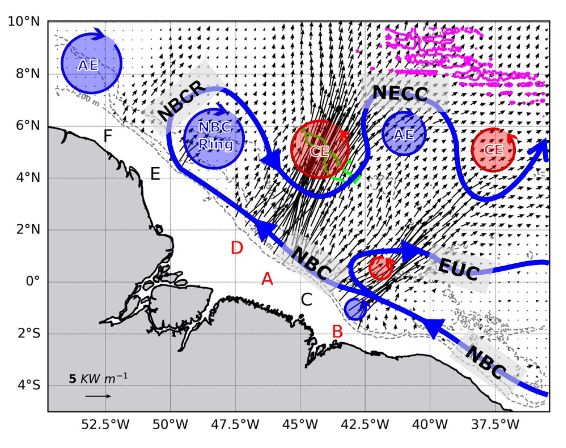
Figure 1 Internal tide generation and propagation, and regional circulation off the Amazon shelf. Key IT generation sites (A–F) are marked along the shelf break, with the three primary sites (A, B, and D) highlighted in red. The associated M₂ baroclinic energy flux, represented by black arrows, is the 25 h mean depth-integrated flux from the September–December (SOND) 2015 period. The schematic background circulation includes the North Brazil Current (NBC), its retroflection (NBCR), North Equatorial Countercurrent (NECC), and Equatorial Undercurrent (EUC) (solid blue lines). Mesoscale eddies are indicated by cyclonic (CEs, red circles) and anticyclonic eddies (AEs, blue circles), the latter including the NBC Ring. Topography, from the NEMO-AMAZON36 model, is detailed with the 200 and 2000 m isobaths (grey lines) and specific features outlined by their 3500 m isobath (Ceará Rise seamount: green contour; Mid-Atlantic ridge: magenta contour).

The region off the Amazon shelf is a dynamic region with a strong western boundary current (North Brazil Current, NBC), receiving large amounts of freshwater from the Amazon and Para Rivers. The area is also marked by high mesoscale activity (MEs), and the presence of seamounts, ITs, and ISWs (Fig. 1). The NBC flows northwestward, exhibiting a seasonal double retroflection eastward, a first one into the North Equatorial Counter-Current (NECC) at about 5–8° N near 50° W, and a second one into the Equatorial Undercurrent (EUC) in winter–spring (Didden and Schott, 1993). Shear instabilities within these currents and their interaction with the Amazon slope generate the CEs and AEs (NBC rings) in this region (Fratantoni and Glickson, 2002; Barnier et al., 2001; Silva et al., 2009). From August to December (ASOND), mean currents and eddy kinetic energy (EKE) are stronger, and the pycnocline is deeper and weaker than during the March-to-July (MAMJJ) season (Aguedjou et al., 2019; Barbot et al., 2021; Tchilibou et al., 2022). Generated at multiple sites (A to E, Fig. 1) along the Amazon shelf break (Tchilibou et al., 2022; Assene et al., 2024; Magalhaes et al. 2016), ITs from the most energetic sites (A and D, Fig. 1) can either propagate over long distances or interact with other processes to potentially disintegrate into ISWs, which have been observed via in situ measurements (Brandt et al., 2002), SAR imagery (Magalhães et al., 2016), MODIS (de Macedo et al., 2023), and SWOT data (Goret et al., 2026). This makes the region an ideal laboratory for studying the tidal variability of IT responses during the propagation of tidal flux.

Using numerical modeling, Tchilibou et al. (2022) reported that the M₂ coherent baroclinic tidal flux propagates more northward during MAMJJ in the region off the Amazon shelf. During ASOND, however, it becomes incoherent – branching and deviating near 6° N – due to strong interactions with MEs and background currents off the Amazon shelf. This variability in flux behavior (e.g., free propagation, refraction, branching) during ASOND may result from the interaction of the coherent flux with MEs, sheared currents (e.g., NECC), changes in stratification, topography (e.g., Ceará Rise seamount, Mid-Atlantic ridge; Fig. 1), other internal wave sources, or coupled processes.

Motivated by the complex mesoscale interplay off the Amazon shelf, we investigate the fate of IT within this dynamic environment at daily timescales from the realistic model outputs. Specifically, we examine whether ITs propagate freely, are deviated, or become trapped by mesoscale features. We further determine whether these outcomes depend on the vertical modes of ITs, or the location of the ME encounters together with its associated background conditions (currents and stratification), distinguishing, for instance, between interactions at a CE core versus its edge. Finally, we explore the synergistic roles of topography (e.g., Ceará Rise seamount) and CEs in governing modal energy transfers.

2 Methodology

2.1 High-resolution numerical model: AMAZON36

We use outputs from the Nucleus for European Modelling of the Ocean (NEMO) model v4.0.2 (Madec et al., 2019), specifically the AMAZON36 configuration (Assene et al., 2024). This high-resolution ($\mathrm{1}/\mathrm{36}$°, ∼ 3 km) model is designed for the western tropical Atlantic (54.7–35.3° W, 5.5° S–10° N) and features 75 vertical layers, with 23 levels in the upper 100 m. The 3 km horizontal resolution provides approximately 30–60, 20–28, and up to 17 grid points per wavelength for Mode-1, Mode-2, and Mode-3 M₂ IT in the Amazon region, corresponding to horizontal wavelengths of ∼ 90–180, ∼ 60–85, and up to ∼ 50 km, respectively (Tchilibou et al., 2022). This resolution ensures that all three modes are well resolved and accurately represents the topography critical to their generation and propagation from the Amazon shelf break (Assene et al., 2024). The latter detailed more about the AMAZON36 configuration parameters.

The model simulations span 11 years, from January 2005 to December 2015, and provides three-dimensional daily and hourly outputs. This dataset has previously been used to study IT interactions with background currents and stratification, as well as IT impact on the ocean thermal structure (Assene al., 2024; Kouogang et al., 2025).

For this study, we focus on the period from September to December (SOND) 2015, when stronger mean currents and EKE contribute to more incoherent ITs (Tchilibou et al., 2022). To analyze the rapid variability of IT responses to MEs like CEs, we examine 25 h segments, from hourly outputs, within the entire SOND season.

2.2 Internal Tides and Mesoscale Activity

Our analysis for each 25 h window of AMAZON36 outputs during the SOND period involves several steps: extracting the M₂ IT constituent, separating the barotropic and baroclinic components, projecting the baroclinic components onto vertical modes, extracting MEs and characterizing their properties, and examining the mean background current pattern and topographic features.

2.2.1 Undecomposed IT Energy equations

First, to examine the variability of IT responses to MEs, we explore all 25 h snapshots of IT energy flux from the AMAZON36 outputs during the SOND period. Following the method of Kelly et al. (2010), barotropic and baroclinic tidal constituents were separated. This separation is performed directly by the NEMO model to ensure accuracy, providing the total energy for all resolved propagation modes at a given tidal frequency (Tchilibou et al., 2022). Our analysis focuses solely on the M₂ harmonic, the dominant tidal constituent in this region (Gabioux et al., 2005; Fassoni-Andrade et al., 2023).

The energy budget for IT can be expressed from the following equations (Wang et al., 2016; Buijsman et al., 2012; Kerry et al., 2013; Tchilibou et al., 2022; Siyanbola et al. 2024):

$$\begin{array}{}\text{(1)}& {\mathrm{\nabla }}_h\cdot \mathit{F}+D+R=C\end{array}$$

In contrast to energy budgets decomposed into vertical modes, we refer to these as the undecomposed IT energy equations. Here, ∇_h⋅F is the divergence of the depth-integrated energy flux, $\mathit{F}=(F_x,F_y$) the energy flux vector, C represents the depth-integrated barotropic-to-baroclinic energy conversion, and D is the depth-integrated energy dissipation term. The term R includes the energy tendency term, implicit horizontal dissipation, wave-mean flow and wave-wave interaction terms, and other offline computation errors. ${\mathrm{\nabla }}_h=(\frac{\partial }{{\partial }_x},\frac{\partial }{{\partial }_y}$) is the horizontal gradient operator.

In the following, a particular attention is given to depth-integrated and time-averaged energy flux term F, which was defined as (Tchilibou et al., 2022; Assene et al. 2024):

$$\begin{array}{}\text{(2)}& [{\mathit{F}}_{\text{bc}},{\mathit{F}}_{\text{bt}}]=\left[\underset{-H}{\overset{\mathit{\eta }}{\int }}{\mathit{u}}_{\text{bc}}{p}_{\text{bc}}\mathrm{d}z,{\mathit{u}}_{\text{bt}}{p}_{\text{bt}}\right],\end{array}$$

where $\mathit{u}=(u,v)$ is the horizontal tidal velocity vector, and p the tidal pressure. Here, the subscripts bt and bc denote barotropic and baroclinic components, respectively. η is the sea surface height and H is the seafloor depth.

2.2.2 Projection of IT Motions Onto Vertical Modes

Second, to investigate whether the IT responses to MEs is mode-dependent and to examine potential inter-modal energy transfer, we project the M₂ tidal constituent onto a set of vertical modes for selected 25 h snapshots that capture ME-induced IT responses. This selective approach substantially reduces the computational cost associated with processing high-resolution 3D data for all 25 h windows during the SOND period.

Vertical Mode Decomposition

For each selected snapshot, we first extract the M₂ harmonic via harmonic analysis. Although performing harmonic fits over short (25 h) segments may introduce frequency leakage from nearby tidal constituents (e.g., S₂, N₂, and K₂) into the M₂ signal, this effect is expected to be small in our case because the tidal regime is strongly M₂-dominated, accounting for more than 70 % of the total tidal energy (e.g., Gabioux et al., 2005; Tchilibou et al., 2022; Fassoni-Andrade et al., 2023). This approach is consistent with previous studies that have successfully applied harmonic analysis to similarly short records to resolve semidiurnal constituents (e.g., 17–29 h M₂ tidal observations in Waterhouse et al., 2018), demonstrating that dominant semidiurnal tides can be reliably estimated from short-duration data.

We then decompose the M₂ tidal currents and pressure using a locally computed set of vertical modes. This method provides a more accurate separation of barotropic and baroclinic tides than simpler approaches (Kelly, 2016; Lahaye et al., 2020; Lahaye et al., 2024; Siyanbola et al. 2024).

The vertical modes are obtained by solving the standard Sturm–Liouville eigenvalue problem at each horizontal grid point, using the local mean stratification profile (based on the time-mean buoyancy frequency, $\stackrel{\mathrm{‾}}{N^{\mathrm{2}}}$), and assuming a flat bottom, a free surface, and no background flow (Gerkema and Zimmerman, 2008; Bella et al., 2024):

$$\begin{array}{}\text{(3)}& {\partial }_z\left({\displaystyle \frac{{\partial }_z{\mathrm{\Phi }}_n}{\stackrel{\mathrm{‾}}{N^{\mathrm{2}}}}}\right)+{\displaystyle \frac{{\mathrm{\Phi }}_n}{c_n^{\mathrm{2}}}}=\mathrm{0},\end{array}$$

with the boundary conditions:

$$\begin{array}{}\text{(4)}& {\partial }_z{\mathrm{\Phi }}_n=\mathrm{0}\text{ at }z=-H,\text{ and }g{\partial }_z{\mathrm{\Phi }}_n+\stackrel{\mathrm{‾}}{N^{\mathrm{2}}}{\mathrm{\Phi }}_n=\mathrm{0}\text{ at }z=\stackrel{\mathrm{‾}}{\mathit{\eta }},\end{array}$$

where ∂_z denotes the partial derivative in z-direction, Φ_n is the horizontal velocity/pressure eigenfunction for mode n, c_n is the modal phase speed and g is the acceleration due to the gravity. The associated vertical velocity/buoyancy eigenfunction, φ_n, is given by:

$$\begin{array}{}\text{(5)}& {\partial }_z{\mathit{\phi }}_n={\mathrm{\Phi }}_n,\text{ and }{\partial }_z{\mathrm{\Phi }}_n=-{\displaystyle \frac{\stackrel{\mathrm{‾}}{N^{\mathrm{2}}}}{c_n^{\mathrm{2}}}}{\mathit{\phi }}_n.\end{array}$$

It should be noted that the flat-bottom assumption could represent a limitation for higher-mode projections near steep topography such as the Ceará Rise seamount. The errors associated with this approximation are expected to be of a few percent for the dominant low modes (Kelly, 2016).

The vertical modes satisfy the orthogonality condition (Kelly, 2016; Lahaye et al., 2024; Bella et al., 2024):

$$\begin{array}{}\text{(6)}& \underset{-H}{\overset{\stackrel{\mathrm{‾}}{\mathit{\eta }}}{\int }}{\mathrm{\Phi }}_m{\mathrm{\Phi }}_n\mathrm{d}z=H{\mathit{\delta }}_{mn},\end{array}$$

where δ_mn is the Kronecker delta and $\stackrel{\mathrm{‾}}{\mathit{\eta }}$ is the time-averaged sea surface height.

We solved Eq. (3) for the first 11 modes ($n=\mathrm{0},\mathrm{1},\mathrm{\dots },\mathrm{10}$) at each grid point, where n = 0 represents the barotropic mode. In this study, the analysis of energy flux focuses primarily on the first three baroclinic modes (n = $\mathrm{1},\mathrm{2},\mathrm{3}$), which are the most dynamically significant at the model's resolution (∼ 3 km). These three baroclinic modes account for 96.2 % (33.2 %), 96.8 % (37.9 %), and 97.2 % (26.3 %) of the total baroclinic energy flux (relative to the combined baroclinic and barotropic flux) in the NE, CEC, and CEE cases, respectively. They therefore capture the dominant share of the baroclinic energy, supporting their use as the basis of our analysis.

The horizontal tidal velocity u and pressure p fields are projected onto these modes to obtain the depth-independent modal amplitudes:

$$\begin{array}{}\text{(7)}& \begin{array}{rl}\left[{\mathit{u}}_n\right(\mathit{x},t),p_n(\mathit{x},t\left)\right]=& {\displaystyle \frac{\mathrm{1}}{H}}\underset{-H}{\overset{\stackrel{\mathrm{‾}}{\mathit{\eta }}}{\int }}\left[\mathit{u}\right(\mathit{x},z,t),p(\mathit{x},z,t\left)\right]\\ & \times {\mathrm{\Phi }}_n(\mathit{x},z)\mathrm{d}z,\end{array}\end{array}$$

with $\mathit{x}=(x,y)$ denoting the horizontal direction.

The full 3D structure of u_n fields for each mode can be reconstructed as (Li et al., 2024):

$$\begin{array}{}\text{(8)}& {\mathit{u}}_n(\mathit{x},z,t)={\mathit{u}}_n(\mathit{x},t){\mathrm{\Phi }}_n(\mathit{x},z).\end{array}$$

Modal Energy Budget

To analyze the inter-modal energy transfer/scattering and redistribution, we examine the terms of the modal energy budget of a given mode interacting with physical features such as topography and mesoscale flow (Fan et al., 2024; Bella et al., 2024; Kelly, 2016; Kelly and Lermusiaux, 2016):

$$\begin{array}{}\text{(9)}& \begin{array}{rl}{\mathrm{\nabla }}_h\cdot {\mathit{F}}_m+D_m+{\mathrm{\Psi }}_m=& {\sum }_n({\mathit{C}}_{mn}+{\mathit{A}}_{mn}+{\mathit{H}}_{mn}\\ & +{\mathit{V}}_{mn}+{\mathit{B}}_{mn}).\end{array}\end{array}$$

Here:

• C_mn is the nonlinear scattering (from mode m>0 into mode n) of energy by topography and stratification.

• A_mn represents the advection of the ITs by the background flow and MEs.

• H_mn and V_mn represent the effect of the horizontal and vertical shear of the background flow, respectively.

• F_m=Hp_mu_m is the depth-integrated and time-averaged baroclinic energy flux for mode m.

• B_mn consist of the three-way interaction term and the horizontal gradient of the buoyancy field.

• Ψ_m consists of the energy tendency terms.

• D_m is the dissipation term of modal energy budget, which also includes interactions with unresolved modes, other physical dissipation processes leading to local dissipation (Alford and Zhao, 2007), and other offline computation errors.

A previous seasonal-scale study by Bella et al. (2024) found the nonlinear coupling terms C_mn, A_mn, H_mn, and V_mn to be dominant across the North Atlantic basin. For our investigation on a daily timescale, a preliminary analysis identified C_mn and H_mn as the dominant terms in our study region. We therefore focus on estimating these dominant couplings terms as defined by Bella et al. (2024):

$$\begin{array}{}\text{(10)}& {\displaystyle }& {\displaystyle }{\mathit{C}}_{mn}=\langle H{p}_m{\mathit{u}}_n\cdot {\mathit{T}}_{nm}-H{p}_n{\mathit{T}}_{mn}\cdot {\mathit{u}}_m\rangle ,\text{(11)}& {\displaystyle }& {\displaystyle }{\mathit{H}}_{mn}=\langle -H\left({\mathit{U}}_{mn}^h{\mathit{u}}_n\right)\cdot {\mathit{u}}_m\rangle ,\end{array}$$

With ${\mathit{T}}_{mn}=\frac{\mathrm{1}}{H}{\int }_{-H}^{\stackrel{\mathrm{‾}}{\mathit{\eta }}}{\mathrm{\Phi }}_m{\mathrm{\nabla }}_h\left({\mathrm{\Phi }}_n\right)\mathrm{d}z$, $({\mathit{U}}_{mn}^h{)}_{ij}=\frac{\mathrm{1}}{H}{\int }_{-H}^{\stackrel{\mathrm{‾}}{\mathit{\eta }}}{\mathrm{\Phi }}_m{\mathrm{\Phi }}_n\frac{\partial {\stackrel{\mathrm{‾}}{U}}_{h,i}}{\partial x_j}\mathrm{d}z$.

Here, the angle bracket 〈⋅〉 denotes the average over a M₂ tidal period, ${\stackrel{\mathrm{‾}}{\mathit{U}}}_h=(\stackrel{\mathrm{‾}}{U},\stackrel{\mathrm{‾}}{V}$) is the time-averaged total horizontal velocity vector. $\frac{\partial {\stackrel{\mathrm{‾}}{\mathit{U}}}_{h,i}}{\partial x_j}$ is the tensor.

The modal horizontal kinetic energy (HKE_n) of M₂ IT is estimated as (Kelly et al., 2012; Fan et al., 2024):

$$\begin{array}{}\text{(12)}& {\text{HKE}}_n={\displaystyle \frac{{\mathit{\rho }}_{\mathrm{0}}H}{\mathrm{2}}}\langle u_n^{\mathrm{2}}+v_n^{\mathrm{2}}\rangle ,\end{array}$$

where ρ₀ is the reference density.

Symmetric–Antisymmetric Separation of Nonlinear Coupling Terms

The energy transfer matrices – including topographic scattering (C_mn) and (H_mn) – are decomposed into symmetric and antisymmetric components, following the established methodology (Savage et al., 2020; Bella et al., 2024). For any general transfer matrix (X_mn), the standard mathematical definitions are: the antisymmetric component, ${\mathbf{X}}_{mn}^{\mathrm{A}}=\frac{\mathrm{1}}{\mathrm{2}}({\mathbf{X}}_{mn}-{\mathbf{X}}_{nm}$), and the symmetric component, ${\mathbf{X}}_{mn}^{\mathrm{s}}=\frac{\mathrm{1}}{\mathrm{2}}({\mathbf{X}}_{mn}+{\mathbf{X}}_{nm}$).

The antisymmetric component, ${\mathbf{X}}_{mn}^{\mathrm{A}}$, represents the internal reallocation of energy – specifically, the scattering or transfer of energy among the various IT vertical modes. Critically, this process conserves the total energy of the IT field, as it analytically redistributes energy across the system modes and spatial scales without introducing a net gain or loss. For instance, the term C_mn is inherently antisymmetric and thus provides a canonical reference for conservative internal energy transfer.

Conversely, the symmetric component, ${\mathbf{X}}_{mn}^{\mathrm{s}}$, describes the net energy exchange between the IT and the low-frequency background flow. When integrated in a basin, this component acts as a source or sink for the IT system, quantifying the total energy gained from or lost to the slowly varying circulation (Bella et al., 2024).

The direction of energy transfer is interpreted from the sign of the matrix elements. Considering a specific mode m:

• For the full matrix X_mn, a negative value indicates a net forward transfer of energy from mode m to mode n, while a positive value indicates a net backward transfer from mode n to mode m;

• For the antisymmetric component ${\mathbf{X}}_{mn}^{\mathrm{A}}$, a negative value signifies a forward transfer from mode m to mode n of the IT field, and a positive value signifies a backward transfer;

• For the symmetric component ${\mathbf{X}}_{mn}^{\mathrm{s}}$, a negative value indicates a forward transfer from mode-m IT to the mode-n background flow, whereas a positive value indicates energy is transferred from the mode-n background flow to mode-m IT.

2.2.3 Eddy detection and structure

Third, to investigate whether the IT responses to MEs depend on the eddy encounter location, including the associated background conditions (currents and stratification), we detected and characterized eddies from 25 h mean snapshots of AMAZON36 outputs during the SOND period.

The mesoscale activity in this region during the 2015 ASOND period was previously assessed by Tchilibou et al. (2022). Their analysis, which compared the model's surface EKE with satellite data, showed reasonable agreement in both the spatial pattern and amplitude of the mean EKE, especially in regions dominated by the NECC.

Eddies were identified in our model outputs using the Okubo–Weiss parameter (W), chosen for its ability to detect coherent vortices on specific isopycnal surfaces or depths (Okubo, 1970; Weiss, 1991; Kurian et al., 2011; Xu et al. 2019). The W parameter is defined as:

$$\begin{array}{}\text{(13)}& W=S_{\mathrm{n}}^{\mathrm{2}}+S_{\mathrm{s}}^{\mathrm{2}}-{\mathit{\zeta }}^{\mathrm{2}},\end{array}$$

where the normal strain (S_n) and shear strain (S_s), and the relative vorticity (ζ) are:

$$\begin{array}{}\text{(14)}& S_{\mathrm{n}}={\displaystyle \frac{\partial u}{\partial x}}-{\displaystyle \frac{\partial v}{\partial y}},S_{\mathrm{s}}={\displaystyle \frac{\partial v}{\partial x}}+{\displaystyle \frac{\partial u}{\partial y}},\mathit{\zeta }={\displaystyle \frac{\partial v}{\partial x}}-{\displaystyle \frac{\partial u}{\partial y}}.\end{array}$$

Regions where rotation (W<0) dominates over strain (W>0) indicate potential eddy cores.

The detection of eddies on selected isopycnal surfaces (between 23 and 27 kg m⁻³ isopycnals) following the procedure of Kurian et al. (2011) and Xu et al. (2019). First, the W fields were smoothed using a 50 km × 50 km half-power filter to suppress small-scale noise. For each 25 h mean snapshot, we then applied a constant threshold of W₀ = −3 × 10⁻¹¹ s⁻² to isolate vorticity-dominated regions (W<W₀). Closed contours corresponding to W=W₀ were identified, and each contour was subjected to a series of quality control criteria to be classified as an eddy: a shape error (deviation from a fitted circle) of less than 50 %, a mean azimuthal velocity greater than 5 cm s⁻¹, and a radius larger than 50 km.

For each identified eddy, its thickness was defined as the vertical extent of its W₀ contours, and its center location was defined as the centroid of the closed W₀ contour. Detected eddies were classified as cyclonic or anticyclonic based on the sign of their potential vorticity anomaly (PVA, positive for CEs and negative for AEs; Fig. 2a).

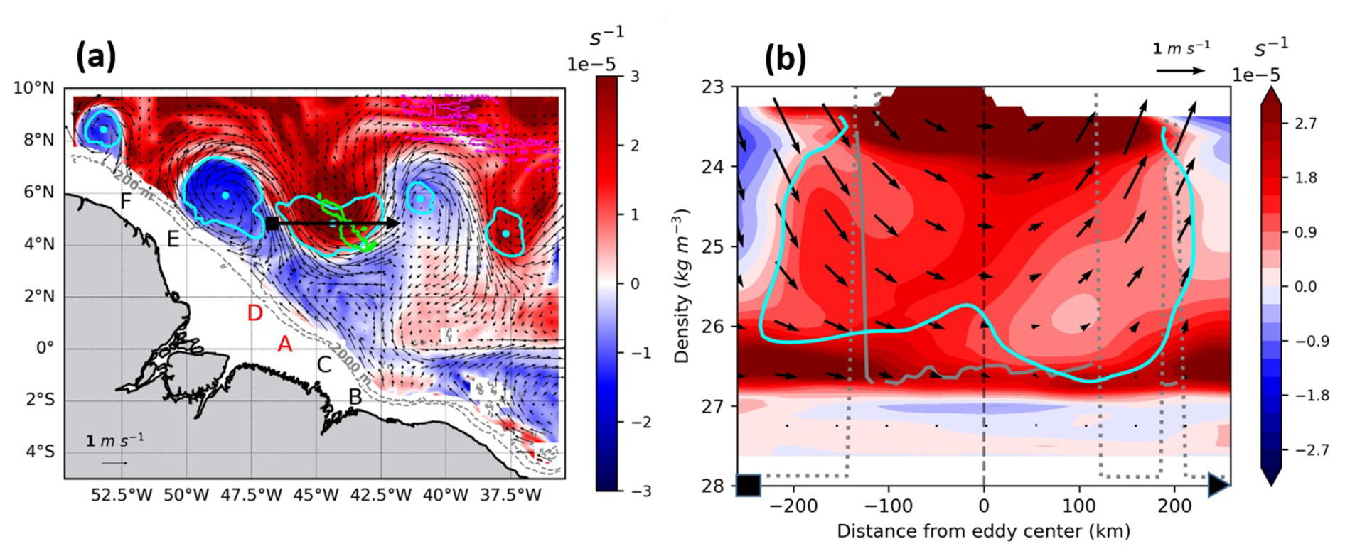
Figure 2 Detection and vertical structure of a representative ME (17 September 2015). (a) PVA (color shading) averaged within the 23–25.5 kg m⁻³ isopycnal layer (∼ 50–160 m depth). Panel (a) shows detected eddy edges (cyan contours), eddy centroids (cyan dots), and mean background currents (black arrows) along the 24 kg m⁻³ isopycnal. (b) Vertical cross-section of PVA along the transect in (a) (black arrow), passing through the core of a CE. The transect endpoints are marked by a square (start) and triangle (end). The vertical dashed black line indicates the eddy centroid, black arrows show the CE-associated currents, and grey lines mark the upper (dotted) and lower (solid) thermocline limits. PVA and mean background currents fields were smoothed using a 50 km × 50 km half-power filter to suppress small-scale noise. Topography is detailed with the 200 and 2000 m isobaths (grey lines) and specific features outlined by their 3500 m isobath (Ceará Rise seamount: green contour; Mid-Atlantic ridge: magenta contour).

To analyze the eddy dynamical structure, we used the framework of rescaled potential vorticity (PV_r). This method filters out high-frequency wave noise to isolate the balanced mesoscale signal. The PV_r is derived from the classical Ertel (1942) potential vorticity, rescaled by a reference stratification at rest, ρ^∗(z), following the approach of Morel et al. (2023, 2019) and subsequent studies (e.g., Delpech et al., 2020; Aguedjou et al., 2021; Ernst et al., 2023).

Its expression is:

$$\begin{array}{}\text{(15)}& {\text{PV}}_r=(\mathrm{\nabla }\times \mathit{U}+f)\cdot \mathrm{\nabla }Z\left(\mathit{\rho }\right)=\mathrm{\nabla }\cdot \left[\right(\mathrm{\nabla }\times \mathit{U}+f\left)Z\right(\mathit{\rho }\left)\right],\end{array}$$

where $\mathit{U}=(\stackrel{\mathrm{‾}}{U},\stackrel{\mathrm{‾}}{V},\stackrel{\mathrm{‾}}{W}$) is the time-mean total velocity vector, and f is the local Coriolis parameter. Z(ρ) is a rescaling function of time-mean potential density ρ, defined using the reference density profile ρ^∗ so that $Z\left({\mathit{\rho }}^{\ast }\right(z\left)\right)=z$. ρ^∗ is defined by the adiabatically rearranged state of minimum potential energy, following the concept of Lorenz (1955) as formalized by Nakamura (1995) and Winters and D'Asaro (1996). An eddy dynamical core is then identified by its anomaly from the background planetary vorticity, $\text{PVA}={\text{PV}}_{\mathrm{r}}-f$, within a layer bounded by two isopycnals.

To distinguish subsurface eddies from surface-intensified ones, we classified them based on the isopycnal level of their core of PVA. Following the method of Kouogang et al. (2025), we used the base of the pycnocline (defined by ∼ 26.5 kg m⁻³ isopycnal) as the boundary of the lower pycnocline depth. Eddies with their PVA core on isopycnals less dense than 26 kg m⁻³ were classified as surface-intensified eddies (Fig. 2b), while those with their core on denser isopycnals (> 26.5 kg m⁻³) were classified as subsurface-intensified eddies as formalized by Aguedjou et al. (2021) in the tropical Atlantic Ocean. This classification scheme was applied to all eddies detected during the SOND period. This study focuses specifically on these surface-intensified eddies.

3 Results

In order to examine the variability of IT responses to MEs, particularly to CEs, we first present three representative cases of interactions between the (non-modal) baroclinic energy flux of the M₂ IT and the detected eddy fields, identified from all 25 h mean snapshots during SOND 2015. We then analyze the IT's vertical mode responses, focusing on the encounter location of the fluxes – originating from the most energetic generation sites A and D – with a CE along their path, and examine the potential modal energy transfer and redistribution.

3.1 Variability of IT responses to MEs: three distinct cases

Following the method described in Sect. 2.2.1 and 2.2.3 (Eqs. 1, 2 and 13–15), we identified three distinct cases from the SOND 2015 period for analysis, each occurring near a spring tide maximum to ensure comparably high tidal energy levels (Fig. 3). This setup minimizes the influence of tidal variability, allowing us to isolate the eddy-induced effects. Although the tidal forcing is not strictly identical across the three cases, the differences in tidal amplitude remain small (less than 18 %) and are therefore considered secondary compared to the large contrasts in mesoscale conditions between the cases.

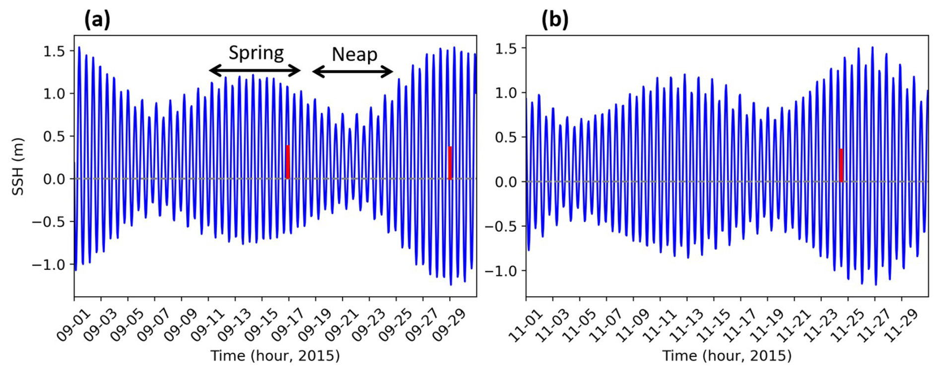
Figure 3 Sea surface height (SSH) from AMAZON36 simulations (station location: 1.29° N, 46.34° W) in (a) September and (b) November 2015. Red bars denote the three case study dates, and black arrows mark the spring-neap tidal cycle.

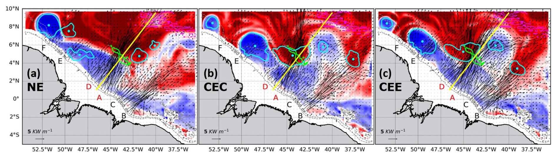
Figure 4 Depth-integrated M₂ total baroclinic energy flux (black arrows) and isopycnally-averaged PVA (color shading), for the (a) NE, (b) CEC, and (c) CEE cases. All fields are 25 h mean snapshots. The PVA is averaged within the 23–25.5 kg m⁻³ density layer (approximately 50–160 m). Detected eddies along the 24 kg m⁻³ isopycnal are overlaid, with edges (cyan contours) and centroids (cyan dots). The respective dates are 24 November 2015 (a), 17 September 2015 (b), and 29 September 2015 (c). The transects (yellow lines) highlight the most energetic energy flux pathways considered, originating from sites A and D. These transects are identical across all three cases to facilitate direct comparison. Topography is detailed with the 200 and 2000 m isobaths (grey lines) and specific features outlined by their 3500 m isobath (Ceará Rise seamount: green contour; Mid-Atlantic ridge: magenta contour).

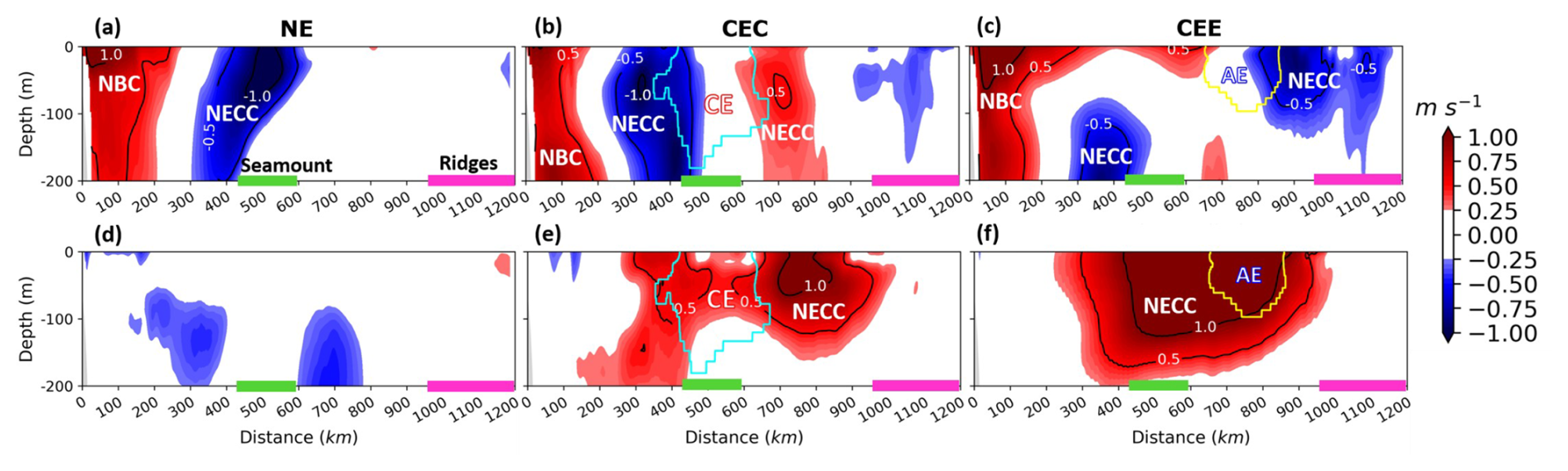
Figure 5 Vertical structure of the mean background current velocity (color shading and black contours) in the upper 200 m, shown along transects defined on the IT propagation paths from sites A and D (Fig. 4). The cross-transect (a–c) and along-transect (d–f) components of current velocity are shown for the NE (a, d), CEC (b, e), and CEE (c, f) cases. In (a)–(c), positive (negative) values indicate flow oriented approximately northwestward (southeastward). In (d)–(f), positive (negative) values indicate flow oriented approximately northeastward (southwestward). Notable topographic features are outlined by colored rectangles (seamount: green; ridges: magenta). Panels (b), (c), (e), and (f) also show the detected eddy edges for AE (yellow) and CE (cyan).

Figure 4 illustrates in the three relevant cases, the M₂ baroclinic energy flux, and detected MEs and their polarity given by the sign of PVA. The three selected cases are located in a region shaped by two major topographic features: the Ceará Rise seamount (∼ 500 km from sites A and D; between 4–6° N, 45–42.5° W), with an amplitude (h_max) of ∼ 1000 m and a width (w_max) of ∼ 100 km, and the Mid-Atlantic Ridge (∼ 1100 km from sites A and D). Each case was selected to highlight distinct IT responses:

• No-Eddy case (NE, 24 November 2015): Energy flux from the primary generation sites (A and D) propagated freely, crossing the seamount and reaching the ridge. A similar pattern was observed from site B (Fig. 4a);

• Cyclone Eddy Center case (CEC, 17 September 2015): Energy flux from sites A and D was refracted into a single beam at the core of a CE positioned (4.9° N, 44.4° W) above the seamount. Separately, flux from the less energetic site E was also refracted into a single beam, emanating from the center of a nearby AE (centered at 5.9° N, 48.5° W) (Fig. 4b);

• Cyclone Eddy Edge case (CEE, 29 September 2015): Energy flux from sites A and D was diffracted into multiple beams at the eastern edge of a CE located (5.3° N, 45.0° W) on the northern flank of the seamount (Fig. 4c).

Across the three selected cases, the analysis of the background conditions (stratification and currents) along a transect following the IT paths from sites A and D reveals strong background currents (> 1.0 m s⁻¹, Fig. 5). In the NE case (Fig. 5a and d), these currents are dominated by their cross-transect component (Fig. 5a), associated with the NBC near the Amazon shelf-break and with the NECC near the seamount. In the eddy cases, the background currents at the CE encounter location differs between cases: in the CEC case (Fig. 5b and e), the currents have both cross- and along-transect components, whereas in the CEE case (Fig. 5c and f), they are dominated by their along-transect component (Fig. 5f). In both eddy cases, the currents at the CE encounter location are associated with the coupled NECC/CE flow. Away from the CE encounter location and the seamount, the background currents exhibit a strong along-transect component associated with the NECC coupled with circulation from a nearby small AE. Regarding background stratification, the horizontal gradient of the mean buoyancy frequency ($\mathrm{\nabla }\stackrel{\mathrm{‾}}{N^{\mathrm{2}}}$, Appendix A, Fig. A1) along the IT paths from sites A and D shows strong signatures ($O({\mathrm{10}}^{-\mathrm{8}}{\mathrm{m}}^{-\mathrm{1}}{\mathrm{s}}^{-\mathrm{2}}$)) localized near topographic features (seamount and ridges). At the CE encounter and seamount locations in the eddy cases, the horizontal stratification gradient is also similarly strong, except in the CEC case where it is quasi-uniform (Appendix A, Fig. A1). The strong background stratification is associated with the NECC in the NE case and with the coupled NECC/CE in the CEC case. Overall, the key distinction between the eddy cases lies not only in where the IT beam encounters the eddy (eddy core vs. eddy edge), but also in the associated background conditions (currents and stratification).

It should be noted that the eddy core/center and eddy edge are defined as regions where $r/R\approx \mathrm{0}$ and $r/R\approx \mathrm{1}$, respectively, where r is the distance from the eddy centroid and R is the radius of maximum velocity. This geometric difference in the CE encounter location leads to markedly different energetic behavior, as discussed below.

In this study, the three cases are qualitatively distinguished by the presence or absence of a CE, and, when a CE is present, by the geometry of the IT–CE intersection.

To determine whether the IT response patterns depend on the IT's vertical structure or on the eddy encounter location, we focus on the IT response to CEs and project the energy flux into vertical modes (Sect. 2.2.2). This approach enables us to examine the specific response of each vertical mode to the CE and potential modal energy redistribution and transfer resulting from these interactions.

3.2 IT Responses to CEs

Following the method described in Sect. 2.2.2 (Eqs. 3–12), we separately analyze the first three vertical modes of the M₂ IT in the three cases.

3.2.1 NE Case: IT without Eddy

We first analyse the tidal energy diagnostics for the NE case to establish an eddy-free propagation baseline. Figure 6a–c maps the energy flux propagation and HKE for the first three modes, revealing distinct patterns for each one.

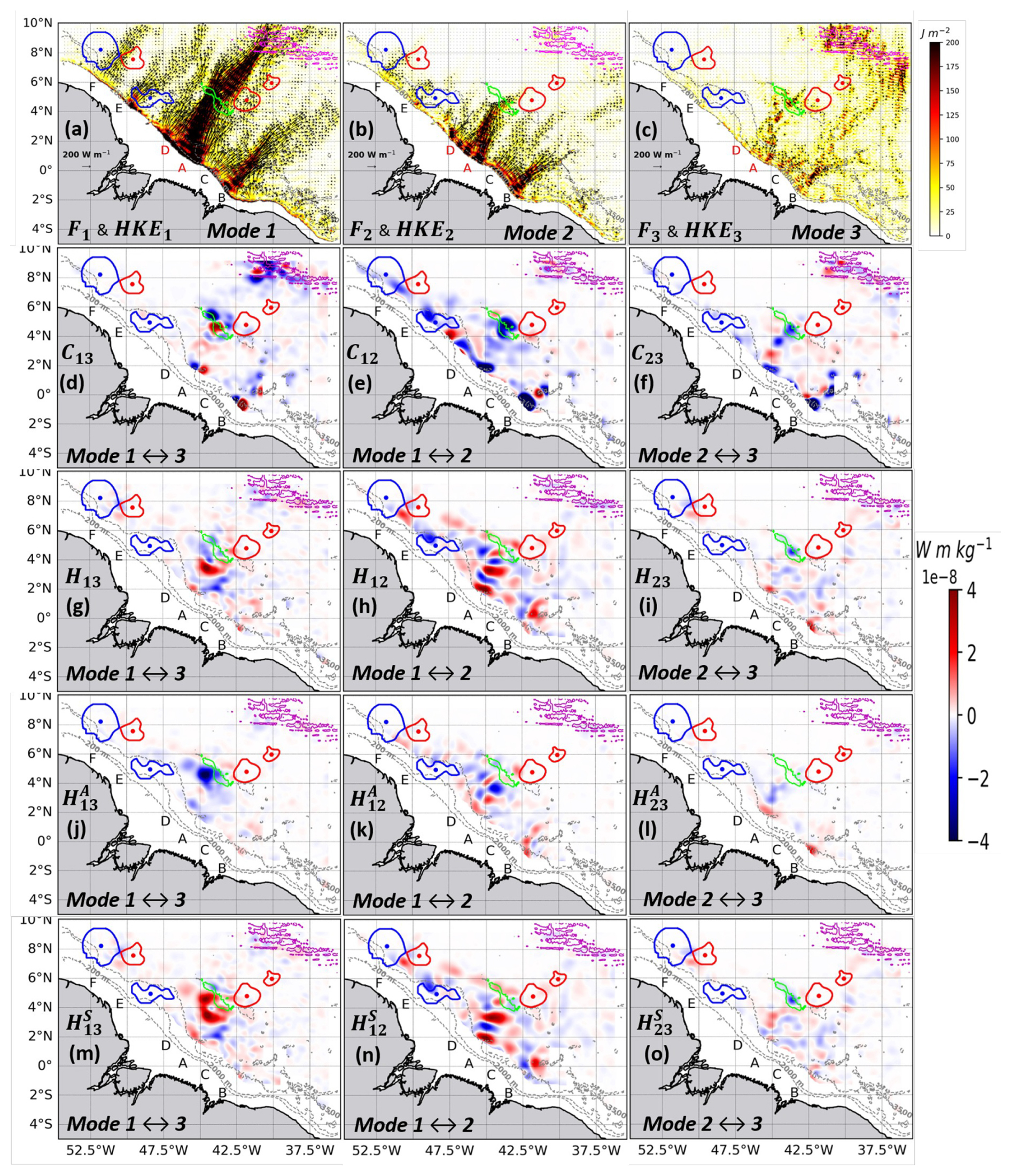
Figure 6 Tidal energy diagnostics for the NE case on 24 November 2015, averaged over a M₂ tidal period. Panels (a)–(c) show the depth-integrated M₂ baroclinic energy fluxes (F_m; black arrows) and horizontal kinetic energy (HKE_m; color shading) for (a) mode-1 (F₁, HKE₁), (b) mode-2 (F₂, HKE₂), and (c) mode-3 (F₃, HKE₃). Panels (d)–(f) present the effects of topographic scattering and stratification (C_mn; color shading) for (d) C₁₃, (e) C₁₂, and (f) C₂₃. Panels (g–i) show the net component of horizontal shear induced by the mean background flow (H_mn; color shading) for (g) H₁₃, (h) H₁₂, and (i) H₂₃. Panels (j)–(l) show the antisymmetric component of this horizontal shear (H_mn; color shading) for (j) $H_{\mathrm{13}}^{\mathrm{A}}$, (k) $H_{\mathrm{12}}^{\mathrm{A}}$, and (l) $H_{\mathrm{23}}^{\mathrm{A}}$. Panels (m)–(o) show the symmetric component of horizontal shear (H_mn; color shading) for (m) $H_{\mathrm{13}}^{\mathrm{S}}$, (n) $H_{\mathrm{12}}^{\mathrm{S}}$, and (o) $H_{\mathrm{23}}^{\mathrm{S}}$. All panels include the detected eddy edges (closed contours) and eddy centroids (dots) for anticyclones (blue) and cyclones (red). Topography is shown using the 200 and 2000 m isobaths (grey contours), with specific features highlighted by the 3500 m isobath (seamount: green contour; Mid-Atlantic Ridges: magenta contour). The C_mn and H_mn fields were smoothed with a Gaussian filter (σ = 7 grid points) to aid interpretation. It should be noted that the colorbar range is saturated in panels to enhance the visibility of energy transfer features.

Mode-1 energy propagation is highly dominant. The fluxes, generated from sites A and D, constructively form a notably coherent beam that converges and propagates northeastward (∼ 37° azimuth) for over 1100 km with minimal deviation (Fig. 6a). This long-distance propagation maintains a relatively constant HKE of 150–200 J m⁻², with a wavelength (λ₁) estimated between 90–125 km. In contrast, the Mode-2 flux propagates a significantly shorter distance (500–600 km, λ₂: 60–85 km) and terminates abruptly at the seamount (Fig. 6b). Mode-3 forms no coherent beams but appears as scattered patches extending only 50–100 km (λ₃: 35–50 km; Fig. 6c). Along their respective beams, Mode-1 and Mode-2 exhibit stronger energy flux amplitudes (> 200 W m⁻¹) compared to Mode-3 (< 200 W m⁻¹). The spatial distribution of these modal energy fluxes is consistent with the vertical structure of the corresponding baroclinic velocity profiles (Appendix B, Figs. B1 and B2). A sharp Mode-2 damping is clearly visible over the seamount, while Mode-3 energy appears trapped over the seamount and ridge where the Mode-1 flux diminishes, suggesting that topographic features drive scattering to higher vertical modes.

To quantitatively assess the mechanisms responsible for this energy loss, we compute intermodal energy transfer terms (Eqs. 9–11) and map only the dominant terms in Fig. 5d–o. These dominant terms, of order of magnitude comparable ($O\left({\mathrm{10}}^{-\mathrm{8}}\mathrm{W}\mathrm{m}{\mathrm{kg}}^{-\mathrm{1}}\right)$), are topographic scattering term (C_mn, Eq. 10), and the horizontal shear term (H_mn, Eq. 11) of background flow. They then are separated into its antisymmetric and symmetric part for the analysis. All other background flow-induced energy transfer terms, such as advection and vertical shear, are negligible in comparison ($O\left({\mathrm{10}}^{-\mathrm{10}}\mathrm{W}\mathrm{m}{\mathrm{kg}}^{-\mathrm{1}}\right)$); figures not shown).

The analysis reveals a primary pathway of intermodal energy transfer driven by topographic scattering term (C_mn), which is antisymmetric by construction. Along the IT path from generation sites A and D, a dominant forward energy cascade (|C_mn|∼ 4 × 10⁻⁸ W m kg⁻¹) occurs near major bathymetric features – the shelf break and seamount. Specifically, energy is sequentially transferred from Mode-1 to Mode-2 IT for C₁₂ (Fig. 6e, blue patches), and then from Mode-2 to Mode-3 IT for C₂₃ (Fig. 6f, blue patches). For C₁₃, however, energy exchanges between Mode-1 and Mode-3 IT are bidirectional – energy is both lost and gained – and spatially confined to the vicinity of topographic features (Fig. 6d, blue and red patches). This could stem from the background conditions, particularly the notable effect of the horizontal stratification gradient in the coupling term C_mn (Appendix A, Fig. A1), or the influence of shear in the background flow (NBC, NECC), the effect of which is discussed in detail below.

Decomposing the horizontal shear term H_mn (Fig. 6g–i) into its antisymmetric (Fig. 6j–l) and symmetric (Fig. 6m–o) components shows that its net influence (|H_mn|∼ 4 × 10⁻⁸ W m kg⁻¹) is more due to the symmetric part. This latter facilitates energy exchanges between the background flow and the IT modes along the IT path from the most energetic sites. Indeed, before the seamount, the symmetric terms $H_{\mathrm{12}}^{\mathrm{S}}$ and $H_{\mathrm{13}}^{\mathrm{S}}$ are both strongly dominant in their net effect, while $H_{\mathrm{23}}^{\mathrm{S}}$ is weakly dominant in H₂₃. In this region, energy is strongly transferred from the Mode-2 and Mode-3 background flow to the Mode-1 IT (Fig. 6m and n, red patches). Over the seamount, the symmetric part of H_mn becomes notable. Here, energy transfers are weak overall, but a notable transfer occurs from the Mode-2 IT to the Mode-3 background flow (Fig. 6o, blue patches).

In essence, in the NE case, coherent energy flux from sites A and D converges and propagates until encountering major topographic features (seamounts and ridges). While Mode-1 IT energy propagates over long distances with amplitudes exceeding 200 W m⁻¹, the higher modes behave differently. Mode-2 IT energy, despite having a comparable amplitude to Mode-1, is effectively damped. In contrast, the weaker Mode-3 IT energy (< 200 W m⁻¹) becomes trapped by the topography. The interaction with topographic features, potentially enhanced by the background flow, triggers significant intermodal energy transfer on the order of 10⁻⁸ W m kg⁻¹. This transfer is governed by two primary mechanisms: (1) topographic scattering drives a dominant forward energy cascade through the IT modes (Mode-1 → Mode-2 → Mode-3), and (2) the horizontal shear of the background flow facilitates a direct energy scattering from the Mode-2 and Mode-3 background flow to Mode-1 IT.

3.2.2 CEC Case: IT Encountering a CE Core

We next examine IT responses when the energy flux from sites A and D encounter the core of a surface-intensified CE (CEC case, Fig. 2b). The CE, centered at 4.9° N, 44.4° W above the localized mid-seamount, has a radius of 157 km, maximum velocity 1.35 m s⁻¹, and a core bounded by 23–25.5 kg m⁻³ isopycnals extending ∼ 150 m within the pycnocline.

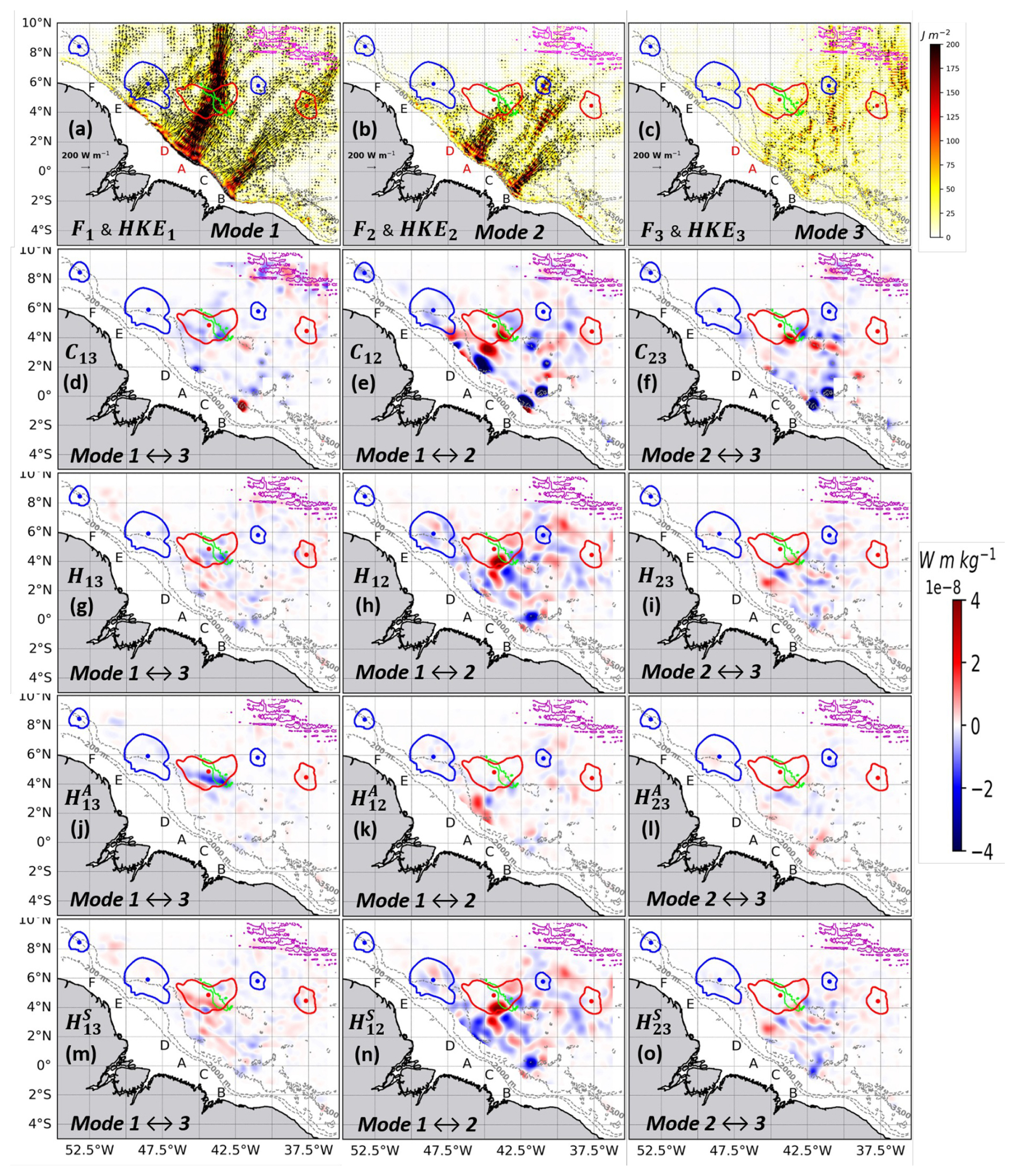
Figure 7 Tidal energy diagnostics for the CEC case (17 September 2015), following the format of Fig. 6.

Prior to interaction, the incident mode-1 IT energy fluxes converge and interfere. Upon encountering the CE core, this energy is refracted into a single beam (Fig. 7a), which emanates from the eddy center and propagates northward at approximately 35° from their northeastward incident direction. Both incident and refracted beams maintain comparable HKE of 150–200 J m⁻² (Fig. 7a), though the refraction process locally confines the energy, leading to a reduction in HKE (25–50 J m⁻²) in the northwestern lee of the eddy. Concurrently, the Mode-2 IT energy flux is blocked at the southern edge of the CE and seamount (Fig. 7b), while Mode-3 appears as scattered patches in the regions where Mode-2 is trapped (Fig. 7c), indicating active intermodal energy scattering. As in the NE case, Mode-1 and Mode-2 IT exhibit higher energy flux amplitudes (> 200 W m⁻¹) along their beams than Mode-3 (< 200 W m⁻¹) (Fig. 7a–c). The  vertical structure of the along-transect baroclinic velocity further supports these results (Appendix B, Figs. B1 and B3).

An analysis parallel to that conducted for the NE case identified the topographic scattering term (C_mn) and the horizontal shear term (H_mn) of the background flow as the dominant mechanisms responsible for the active energy scattering observed.

The analysis of the term C_mn in the CEC case reveals a distinct coupling pattern modulated by the CE core in conjunction with the seamount along the IT path from sites A and D. A dominant forward energy transfer (|C_mn|∼ 4 × 10⁻⁸ W m kg⁻¹) from Mode-1 to Mode-2 occurs near the shelf break for C₁₂ (Fig. 7e, blue patches), consistent with the NE case (Fig. 6e). A significant shift occurs near the southern edge and core of the CE, where a dominant backward energy transfer is observed (with the exception of Mode-1 to Mode-3 IT). Here, energy is sequentially gained by Mode-1 from Mode-2 for C₁₂ (Fig. 7e, red patches near the southern edge and core of the CE) and by Mode-2 from Mode-3 for C₂₃ (inverse cascade, Fig. 7f, red patches), while energy is simultaneously lost from Mode-1 to Mode-3 for C₁₃ (direct forward transfer, Fig. 7d, blue patches). These patterns could be due to either the horizontal stratification gradient in the coupling term C_mn associated with the CE (Appendix A, Fig. A1), or shear in the background flow (NECC/CE).

Analysis of the background flow horizontal shear term (H_mn) shows that its magnitude (|H_mn|∼ 4 × 10⁻⁸ W m kg⁻¹) is comparable to the topography scattering term as in NE case. In the CEC case, along the energy flux from sites A and D, the net effect of H_mn (Fig. 7g–i) is primarily due to its symmetric part (Fig. 6m–o), except for term H₁₃. Between the shelf break and the southern edge of the CE, both the symmetric terms $H_{\mathrm{12}}^{\mathrm{S}}$ and $H_{\mathrm{23}}^{\mathrm{S}}$ are both strongly dominant in their net effect. In this region, energy is both lost and gained between the Mode-1 IT and the Mode-2 background flow, and between the Mode-2 IT and the Mode-3 background flow (Fig. 7n and o, blue patches). This bidirectional transfer is spatially confined to this region and more pronounced between the Mode-1 IT and the Mode-2 background flow, a pattern also present in the NE case (Fig. 6h and n). Near the CE center and seamount, the terms $H_{\mathrm{13}}^{\mathrm{A}}$ and $H_{\mathrm{13}}^{\mathrm{S}}$ weakly combine to form H₁₃ (Fig. 7j and m, blue and red patches), while $H_{\mathrm{12}}^{\mathrm{S}}$ and $H_{\mathrm{23}}^{\mathrm{S}}$ both remain dominant in their net effect. These patterns coincide with the region where energy fluxes are deflected. Here, energy transfer is stronger for $H_{\mathrm{12}}^{\mathrm{S}}$ than for $H_{\mathrm{23}}^{\mathrm{S}}$. Specifically, the background flow loses energy to the IT modes: the Mode-2 background flow energizes the Mode-1 IT (Fig. 7n, red patches), and the Mode-3 background flow energizes the Mode-2 IT (Fig. 7o, red patches). These overall patterns indicate a deflection of Mode-1 and Mode-2 IT, and provide strong evidence for a dominant energy pathway from the background flow to the IT modes driven by horizontal shear. This latter is coupled with direct forward energy transfer between IT modes driven by topographic scattering previously observed.

In summary, in the CEC case, the interaction with the CE core dictates distinct fates for IT modes. Mode-1 IT from sites A and D is not freely propagating but is primarily refracted into a single northward beam. In contrast, Mode-2 IT is blocked, and Mode-3 IT is scattered at the eddy edge and seamount. Energy flux amplitudes for Modes 1 and 2 exceed 200 W m⁻¹ along their beams, whereas Mode-3 remains below this threshold. This interaction facilitates a significant energy transfer ($O(\sim {\mathrm{10}}^{-\mathrm{8}}\mathrm{W}\mathrm{m}{\mathrm{kg}}^{-\mathrm{1}})$) governed by a complex interplay of two mechanisms: (1) a dominant backward energy cascade, where horizontal shear transfers energy from the Mode-3 background flow to Mode-2 IT, and from the Mode-2 background flow to Mode-1 IT; and (2) a forward scattering, where topography directly transfers energy from Mode-1 to Mode-3 IT.

3.2.3 CEE Case: IT Encountering a CE Edge

Finally, we assess IT interactions with the edge of a surface-intensified CE centered at 5.3° N, 45.0° W (radius 143 km, maximum velocity 1.23 m s⁻¹, core bounded by 23–25.5 kg m⁻³ isopycnals extending ∼ 100 m above the pycnocline).

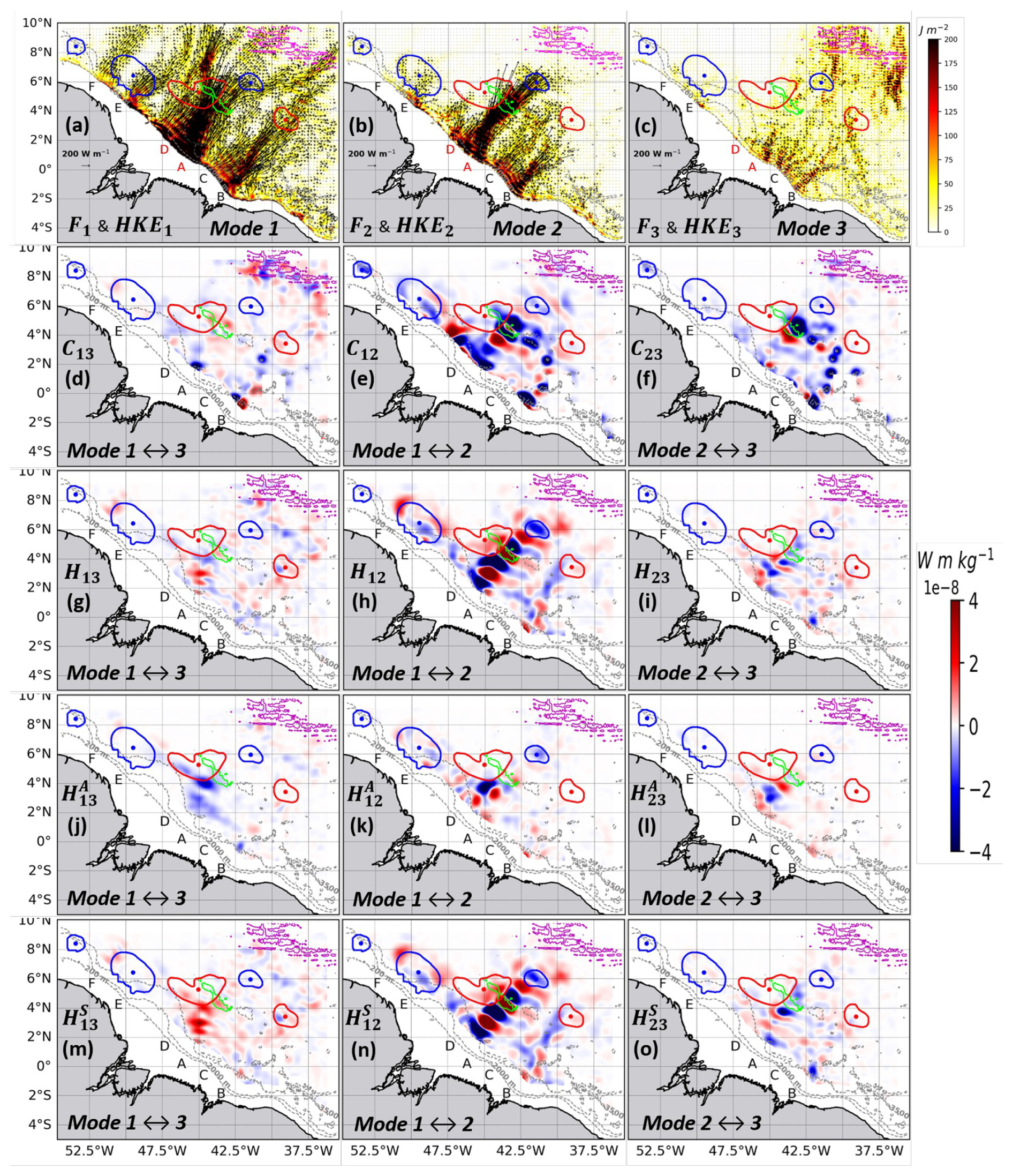
Figure 8 Tidal energy diagnostics for the CEE case (29 September 2015), following the format of Fig. 6.

This interaction yields a different kinematic response. The incident Mode-1 energy fluxes from sites A and D converge and, at the eddy edge, clearly diffract into two distinct beams (Fig. 8a): one propagating northward (∼ 39°) and the other eastward (∼ 35°) relative to their northeastward incident direction. The northward-refracted beam maintains high HKE (150–200 J m⁻²), while HKE is sharply reduced (25–50 J m⁻²) in the northeast lee of the CE (Fig. 8a). Separately, the eastward-refracted beam, less energetic (HKE < 100 J m⁻²) than the northward beam, passes near the eastern edge of a small AE. Mode-2 flux is sheared at the CE edge with limited directional change (Fig. 8b), and Mode-3 becomes trapped along the northeastern CE edge and near the ridge (Fig. 8c). Consistent with previous cases, Mode-1 and Mode-2 exhibit higher energy flux amplitudes (> 200 W m⁻¹) than Mode-3 (< 200 W m⁻¹), and the energy flux patterns is supported by the vertical structures of the baroclinic velocity (Appendix B, Figs. B1 and B4).

As in prior cases, the analysis identified topographic scattering (C_mn) and horizontal shear (H_mn) of the background flow as the two dominant mechanisms driving intermodal scattering in the CEE case.

The analysis of the term C_mn reveals a pattern modulated by the CE edge and seamount along the IT path from sites A and D. A dominant forward energy transfer (|C_mn|∼ 4 × 10⁻⁸ W m kg⁻¹) from Mode-1 to Mode-2 for C₁₂ (Fig. 8e, blue patches) and from Mode-1 to Mode-3 IT for C₁₃ (Fig. 8d, blue patches) occurs near the shelf break. Near the eastern edge of the CE and the southern flank of the seamount, inter-modal IT energy transfers – between Mode-1 and Mode-2 IT, and between Mode-2 and Mode-3 IT – are both strong and bidirectional (i.e., forward and backward transfers coexist; Fig. 8e and f, blue and red patches), and remain spatially confined to this region. An exception is the Mode-1 to Mode-3 IT transfer (Fig. 8d), which is weak in this area.

These overall patterns indicate that the CE edge inhibits the forward energy cascade observed in the NE case and instead initiates a dual mechanism: a potential flow shear-induced energy transfer between the background flow (NECC/CE) and IT modes, and a topographically-driven energy scattering between IT modes.

As in previous cases, the horizontal shear term (H_mn) in the CEE case is of comparable magnitude (|H_mn|∼ 4 × 10⁻⁸ W m kg⁻¹) to the topographic scattering term. The net effect of H_mn (Fig. 8g–i) is primarily dominated by its symmetric part (Fig. 8m–o), except for term H₁₃. Along the IT path from sites A and D, terms $H_{\mathrm{12}}^{\mathrm{S}}$ and $H_{\mathrm{23}}^{\mathrm{S}}$ are both strongly dominant in their net influence, while $H_{\mathrm{13}}^{\mathrm{A}}$ and $H_{\mathrm{13}}^{\mathrm{S}}$ weakly combine to form H₁₃ (Fig. 8g, j, and m) – a pattern also present in the CEC case (Fig. 7g, j, and m). The energy transfer pattern along this path is characterized by alternating bands of energy loss and gain (blue and red patches), reflecting bidirectional transfers between the background flow and IT modes. These alternating bands are particularly striking and spatially extended for $H_{\mathrm{12}}^{\mathrm{S}}$ (Fig. 8h and n). They are distinct from those observed in the previous cases, appearing both upstream and downstream of the seamount and near the eastern CE edge. These patterns could result from an interference structure associated with the IT field. For $H_{\mathrm{23}}^{\mathrm{S}}$, however, forward energy transfer dominates: the Mode-2 IT energizes the Mode-3 background flow near the CE edge (Fig. 8o, blue patches), coinciding with the region where energy fluxes are deflected. These overall patterns provide strong evidence for a dominant energy pathway between the background flow and IT modes driven by horizontal shear, coupled with a topographically-driven energy transfer between IT modes.

In summary, in the CEE case, upon interacting with the CE edge, each IT mode meets a distinct fate. Mode-1 IT from sites A and D splits into two energetic beams, propagating northward and eastward with energy fluxes exceeding 200 W m⁻¹. In contrast, Mode-2 IT is sheared apart, while Mode-3 IT is scattered by the eddy edge and seafloor topography, its energy flux remaining below 200 W m⁻¹. During this encounter, a significant energy transfer (∼ 10⁻⁸ W m kg⁻¹) occurs through dual mechanism distinct from that observed in the CEC case: (1) a dominant bidirectional energy transfer between the background flow and the IT modes (Mode-1 ↔ Mode-2 ↔ Mode-3) driven by horizontal shear, which can act to suppress the topographically-driven downscale energy, and (2) a bidirectional energy transfer between the IT modes driven by topographic scattering.

4 Discussion

This study investigated the fate of M₂ IT energy on the Amazon shelf during the high EKE period of SOND 2015. We addressed three questions: (1) Does the IT propagate freely, deviate, or become trapped by mesoscale features? (2) Do these outcomes depend on the IT vertical mode, or on the location of the ME encounters (CE core vs. edge) along with the associated background conditions (currents and stratification)? (3) What are the synergistic roles of topography and CEs in governing modal energy transfers? By projecting energy flux into vertical modes and performing intermodal energy transfer terms, we dissected these interactions more deeply.

4.1 The Variable Fate of Internal Tides: Free Propagation, Deviation, and Trapping

Our results show that the fate of IT energy is not uniform but is dictated by interactions with mesoscale features, affecting the intensity and distribution of energy flux. The NE case established a baseline of efficient, long-range propagation, where the Mode-1 energy flux maintained amplitudes exceeding 200 W m⁻¹ along a coherent beam for over 1100 km. This free propagation aligns with previous studies (e.g., Xu et al., 2016; Fan et al., 2024) and confirms Mode-1's characteristic as a freely propagating IT (Zhao et al., 2010). Its path is governed by Snell's law (Small, 2001; Zhao, 2014), with minimal Coriolis constraint (f) near the equator ($f/{\mathit{\omega }}_{M_{\mathrm{2}}}$ < < 1, with ${\mathit{\omega }}_{M_{\mathrm{2}}}$ the M₂ tidal frequency), shifting steering mechanisms to wave–current and wave–stratification interactions. The stability of the Mode-1 IT beam in background flow is consistent with ray-tracing results, such as those at the Hawaiian Ridge, where typical currents had only slight effects (Rainville and Pinkel, 2006). While high-resolution and idealized simulations suggested reduced Coriolis constraints at low latitudes (Wang et al., 2021; Le Dizes et al., 2025), our realistic simulations advance these findings by forcing nonlinear interactions in a highly complex field.

In the NE case, the strong background flow – particularly the NECC – moved quasi-perpendicular to the incident Mode-1 IT beams, and the associated stratification was notable over the seamount. The subcritical seamount ($h_{\text{max}}/H\sim$ 0.2) acted only as a minor directional obstacle (${\mathit{\lambda }}_{\mathrm{1}}/w_{\text{max}}\sim$ 0.9–1.25) for propagating Mode-1 IT, though it could affect higher-order modes intensified near the bottom.

In contrast, in the eddy cases, the incident Mode-1 IT beams passed through the strong cross-beam and along-beam background flow (NECC/CE) in the CEC and CEE case, respectively. The presence of a CE consistently disrupted free IT propagation, leading to deviation or trapping with distinct energy modulations. The incident Mode-1 IT was deviated into convergent energy beams, creating a zone of reduced energy flux in the lee of the eddy, consistent with processes modeled by Wang and Legg (2023) and Dunphy and Lamb (2014). This reduction in coherent energy flux is strongly supported by in situ observations south of the Azores, which reported a reduction in low-mode IT energy flux during interactions with a surface-intensified eddy (Löb et al., 2020). Across all cases, Mode-3 energy never formed a coherent beam and consistently exhibited the weakest fluxes (< 200 W m⁻¹). The most relevant blockage occurred for Mode-2 (with flux amplitude comparable to Mode-1) in the CEC case, where an otherwise energetic mode was completely impeded at the eddy–seamount interface. This vulnerability aligns with global observations that Mode-2 M₂ IT generally has smaller sea surface height amplitudes and shorter propagation distances (O[100 km]) than Mode-1 (Zhao, 2018). MEs thus act as potent filters that selectively dissipate or trap the energy of specific vertical modes.

It should be noted that the multi-source interference, observed along the propagation paths of the energy fluxes from sites A and D, could also modify the beam geometry independently of mesoscale activity. In this study, we assume that the contribution of multi-source interference is smaller than that of eddy-induced effects. A more detailed analysis would be required to precisely quantify this contribution.

4.2 The Dual Control of IT Response: Vertical Mode and Eddy Encounters

A key finding of this study is that the IT responses to an ME is dually controlled by its vertical mode, and the specific location of the eddy encounter and its associated background conditions. Mode-1 IT is robust and long-ranging but susceptible to beam steering, while Mode-2 is far more vulnerable to damping and blocking. Mode-3 IT is consistently weak and scattered, behaving as a trapped mode that seldom forms coherent beams. Only Mode-1 IT underwent large-scale deviation by MEs or background flow fields, with energy loss occurring via forward energy transfer at localized, energetic interaction sites (seamount, eddy boundaries). This is consistent with studies showing that remote IT energy is scattered to higher modes at continental margins (Siyanbola et al., 2024; Fan et al., 2024) and with findings that an ME focuses Mode-1 energy flux in specific areas while inducing vertical mode scattering (Dunphy and Lamb, 2014). Our observation of Mode-1 deviation is analogous to the redirection of ISWs by ME fields (Liao et al., 2012; Goret et al., 2026).

IT beam deviation is sensitive to eddy properties. The direction of deviation depends strongly on eddy polarity, as shown by previous studies (e.g., Huang et al., 2018; Guo et al., 2023; Dunphy et al., 2017; Wang and Legg, 2023; Li et al., 2024; Goret et al., 2026). While the present study focuses exclusively on CEs, a qualitative illustration of AE-induced deflection can be glimpsed in the energy flux path emanating from the less energetic generation site E (Fig. 4b: deviation of the energy flux due to an AE core centered at 5.9° N and 48.5° W). While earlier work noted that AE cores speed up Mode-1 propagation and induce clockwise (southward) refraction, whereas CE cores slow it down and induce counterclockwise (northward) refraction, our findings link specific interaction geometries to distinct intermodal energy pathways in a realistic framework. The impact of AEs on intermodal energy pathways remains an important open question. Based on previous studies (e.g., Dunphy and Lamb, 2014; Goret et al., 2026), we can assume that AEs exhibit a symmetric response; however, precise quantification is left for future investigation.

The distinction between the CEC (core) and CEE (edge) cases reveals that the same CE can impose fundamentally different fates on a passing Mode-1 IT beam. Interaction with the eddy core – where stratification was strong and the CE flow was oriented cross-beam – refracted the incident beam coherently by ∼ 35° into a single northward path. In contrast, an encounter at the eddy edge – where stratification was quasi-uniform and the CE flow was oriented along-beam – diffracted the energy into two distinct beams propagating northward (∼ 39°) and eastward (∼ 35°). This demonstrates that “eddy lensing” is nuanced and sensitive to the radial structure and shear fields of the eddy. Recent SWOT satellite observations corroborate this finding, documenting analogous refraction near an eddy core and diffraction at a western eddy edge within the study region (Goret et al., 2026). Our results provide a mechanistic explanation for incoherent IT signals and variable trapping noted in high-resolution models of the ASOND period in this region (Tchilibou et al., 2022).

While Mode-1 IT is susceptible to beam steering, higher modes (Mode-2 and Mode-3) are more sensitive to topography and are quickly damped, trapped, and become primary recipients of energy via downscale cascades linked to topographic scattering (Lahaye et al., 2020; Fan et al., 2024; Bella et al., 2024). Our results advance these findings by showing that higher modes are also more sensitive to the presence of a CE in conjunction with a localized seamount. Therefore, the energy scattering from lower to higher IT modes and the trapping of those modes by CE's flow are two linked processes facilitating the IT dissipation (Wang and Legg, 2023).

This study was limited to surface-intensified eddies. Future work should investigate whether similar IT interactions occur with other ME types, such as deep intrathermocline eddies or complex multi-eddy systems. A key question is whether eddies with thin vertical structures – and thus higher vertical modes – are capable of trapping ITs, which warrants specific examination.

4.3 Synergistic Roles of Topography, Background Flow, and CEs in Modal Energy Transfers

Our results reveal a complex hierarchy of interactions that governs modal energy transfers, where even without strong MEs, the combined effects of topography and background flow establish a baseline for energy pathways.

The NE case shows the seamount acts as a critical site for modal scattering, driving a dominant forward energy cascade from Mode-1 to Mode-2 to Mode-3 IT (∼ 4 × 10⁻⁸ W m kg⁻¹). This magnitude of transfer is characteristic of interactions over abrupt topography, consistent with quantifications of energy cascades on continental slopes (Kelly et al., 2012). This topographically driven transfer is significantly modulated by background flow (NECC, NBC) through horizontal shear mechanisms of comparable strength, aligning with studies in the North Atlantic concluding that low-frequency flow strongly impacts the IT energy cycle, often transferring energy toward smaller scales (Bella et al., 2024). Background flow shear actively participates in energy exchange, facilitating transfer from the Mode-2 and Mode-3 background flow to the Mode-1 IT before the seamount, and from the Mode-2 IT to the Mode-3 background flow over the seamount. Thus, the interaction between the background flow and the topography creates a dynamic environment for energy redistribution, even before considering ME effects.

Introducing a CE – particularly one co-located with the seamount, as in the CEC case – fundamentally reorganizes the energy transfer landscape. The CE's strong horizontal shear dominates background flow effects and reverses the canonical energy pathway, initiating a dominant inverse energy cascade from background flow to IT modes. This shift from the topographically driven forward cascade observed in the NE case is mediated by horizontal shear, supported by analyses using coupled-mode shallow-water models that emphasize advection terms involving mean flow and buoyancy shear (Kelly et al., 2016). The synergy between the CE and seamount creates competing pathways: topographically driven forward scattering operates concurrently with eddy-driven inverse cascades, leading to complex energy redistribution that explains observed modal blocking and trapping. This aligns with studies detailing how CEs and AEs differently affect topographic scattering (Li et al., 2024) and underscores that cross-scale energy exchange is a key driver in the tropical western Atlantic (Wang et al., 2025).

The consistent co-location of the CEs and the seamount with the NECC suggests the background conditions – specifically western boundary currents – combined with the position of CE encounters, act to further enhance IT refraction and diffraction. This mechanism is supported by studies in other western boundary currents (Duda et al., 2018; Cao et al., 2022; Xu et al., 2021; Kelly and Lermusiaux, 2016; Chen et al., 2022; Pereira et al., 2007; Kelly et al., 2016). However, fully isolating the individual contributions of the eddy flow from that of the NECC will require a future idealized modelling framework.

5 Conclusion

This study illustrates the complex pathways of M₂ IT energy in the region off the Amazon shelf during the period of SOND 2015. By applying vertical mode decomposition to high-resolution NEMO-AMAZON36 simulations, we examined three representative interaction cases: undisturbed propagation until crossing a topography, interaction with a CE core, and interaction with a CE eastern edge. These three cases are schematically represented in the Fig. 9. For each case, we systematically computed the intermodal energy transfer terms to identify the governing mechanisms.

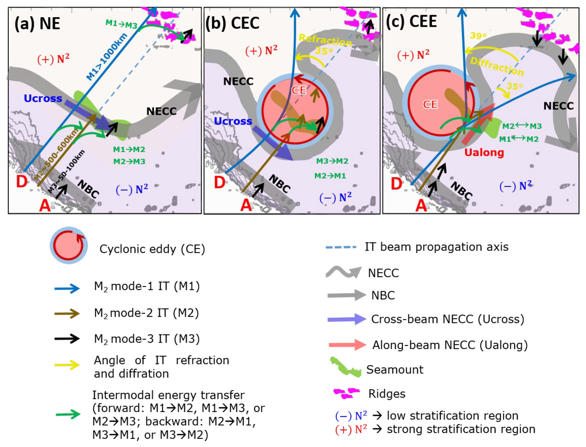
Figure 9 Schematics summarizing the fate of propagating M₂ IT from generation sites A and D on the Amazon shelf-break. The panels correspond to the three analyzed cases: (a) NE, (b) CEC, and (c) CEE. The diagram highlights the key dynamic IT responses – inter-modal scattering, refraction, and diffraction – resulting from interaction with mesoscale structures, emphasizing the pronounced effects of CEs. The specific IT response is dually controlled by its vertical mode, and the CE encounter location along with the associated background conditions. Furthermore, intermodal energy scattering is governed by a hierarchical synergy between the seamount and the CE's background flow.

The two primary conclusions are as follows. First, the specific response of an IT – whether it propagates freely or deviates – is dually controlled by IT vertical modal structure, and the location of the ME encounters together with its associated background conditions (currents and stratification). In the absence of a strong eddy (NE case, Fig. 9a), Mode-1 IT propagated freely as a long-range coherent beam. It passed through the cross-beam NBC flow, crossed the Ceará Rise seamount, and continued through the cross-beam NECC flow – the latter associated with strong stratification – with little disruption. In contrast, interactions with a CE and its associated currents and stratification consistently disrupted this propagation pattern, leading to refraction, diffraction, or trapping. When the beam encountered the CE core (CEC case, Fig. 9b), where stratification was strong and the CE flow was oriented cross-beam, the Mode-1 beam was coherently refracted northward by approximately 35° while maintaining high energy fluxes (> 200 W m⁻¹). At the eddy edge (CEE case, Fig. 9c), however, where stratification was quasi-uniform and the CE flow was oriented along-beam, the beam instead underwent diffraction: its energy split into two distinct beams propagating northward (∼ 39°) and eastward (∼ 35°). Higher modes were particularly susceptible to trapping; Mode-2 energy flux – despite an amplitude comparable to Mode-1 – was completely blocked and trapped at the eddy-seamount interface, while Mode-3 energy remained weak (< 200 W m⁻¹), scattered and less blocked. This weaker and more spatially diffuse signature of mode 3, in contrast to the clearly blocked mode 2, likely reflects local generation near the seamount and/or a loss of coherence induced by the overlying eddy, and deserves future investigation.

Second, the redistribution of energy via intermodal transfers is governed by a hierarchy of synergistic interactions between the seamount and the background flow of the eddy. In the NE case, the seamount drives a dominant forward energy cascade from Mode-1 to higher modes ($O\left({\mathrm{10}}^{-\mathrm{8}}\mathrm{W}\mathrm{m}{\mathrm{kg}}^{-\mathrm{1}}\right)$), a process modulated by the background flow's horizontal shear. The presence of a CE colocated with the seamount fundamentally reorganizes this dynamic. The CE's strong horizontal shear initiates a dominant inverse energy cascade from the background flow to the IT modes, directly competing with the ongoing topographic forward cascade. This specific synergy is crucial for explaining the extreme blocking of Mode-2 and the complex redistribution of energy fluxes observed.

Nonetheless, the region is shaped by a complex, co-located interplay of forces – including the NECC, MEs (CEs and AEs), and the topographic features – making it challenging to fully isolate their individual effects on ITs in our realistic simulations. Limiting our analysis to three case studies reflects the primarily qualitative nature of our approach. A natural next step would be to extend it toward more quantitative results by conducting composite analyses over a larger set of eddy–IT interaction cases. Grouping configurations by eddy position relative to the seamount, for instance, would allow the IT responses to mesoscale variability to be characterized in a statistically robust way. In addition to statistical analyses, to disentangle and quantify the specific contributions of each mesoscale feature with greater precision, future work should also employ idealized modelling frameworks. Such an approach is essential for isolating the deterministic impacts of mesoscale flow and advancing toward a predictive understanding of IT energy pathways in complex oceanic environments.

Finally, it should be noted that the use of flat-bottom vertical modes in the vicinity of steep topography represents a limitation of our analysis, particularly for diagnosing higher-mode energy transfers near the seamount. Future work employing topography-aware modal decompositions would help refine these results and provide a more accurate representation of IT energetics.

Appendix A: Horizontal Stratification Gradients Along IT Paths

To evaluate the background stratification in the NE, CEC, and CEE cases, we computed the horizontal stratification gradient ($\mathrm{\nabla }\stackrel{\mathrm{‾}}{N^{\mathrm{2}}}$) along the transect defined on the IT propagation paths from sites A and D (Fig. 4). The horizontal gradient of the mean buoyancy frequency was strong near the topographic features (seamount and ridges; Fig. A1a–c) and the CE core (Fig. A1b), but quasi-uniform near the CE edge (Fig. A1c).

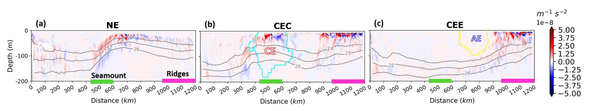
Figure A1 Horizontal gradient of the mean buoyancy frequency ($\mathrm{\nabla }\stackrel{\mathrm{‾}}{N^{\mathrm{2}}}$) in the upper 200 m, shown along transects defined by the IT propagation paths from sites A and D (Fig. 4), for the (a) NE, (b) CEC, and (c) CEE cases. Color shading indicates the gradient magnitude. Notable topographic features are outlined by colored rectangles (seamount: green; ridges: magenta). Panels (b) and (c) also show the detected eddy edges for AE (yellow) and CE (cyan). All panels show selected mean potential density isopycnals (24–26 kg m⁻³, grey contours).

Appendix B: M₂ Tidal Beam Dynamics

To better determine whether the response of ITs to MEs, specifically CEs, is governed more by the IT's vertical structure or by the CE's properties and location, we analyzed the M₂ baroclinic velocity field. Following the methodology in Sect. 2.2.2, we projected the tidal velocity field into vertical modes and defined transects along different IT beams for the NE, CEC, and CEE cases (Fig. B1): the northeastward incident beam (yellow) from sites A and D, northward refracted beams from CE center (green), and diffracted beams (northward and eastward) from CE edge (green). We then decomposed the modal velocities into along- and cross-transect components. The transect along the incident tidal beam was identical in all three cases to enable a direct comparison. Our analysis focused on the more energetic along-transect component, as shown in Fig. B2–B4. The vertical structure of this velocity component was found to be coherent with the modal M₂ energy flux patterns in all analyzed cases.

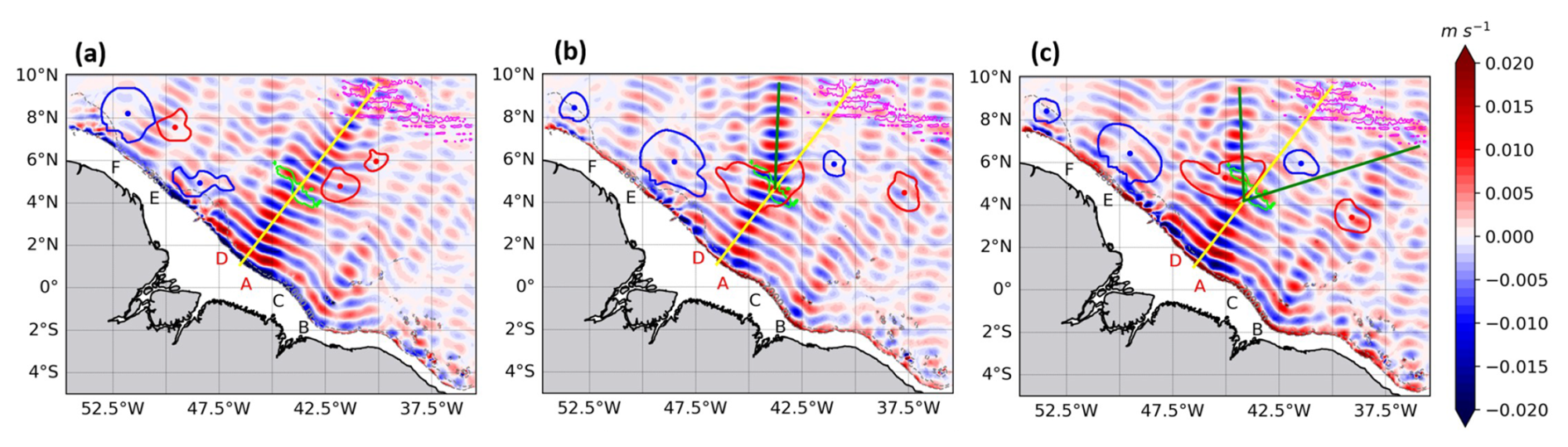
Figure B1 Horizontal propagation of mode-1 M₂ IT beams. Snapshots (at t= 6 h) of meridional baroclinic velocity for the (a) NE, (b) CEC, and (c) CEE cases. The corresponding dates are 24 November, 17 September, and 29 September 2015, respectively. All panels include defined transects along different IT beams: the northeastward incident beam (yellow lines) from sites A and D, northward refracted beams from CE core (solid green line), and diffracted beams (northward and eastward) from CE edge (solid green lines). Detected eddy edges (closed contours) and centroids (dots) for AE (blue) and CE (red) are also shown.

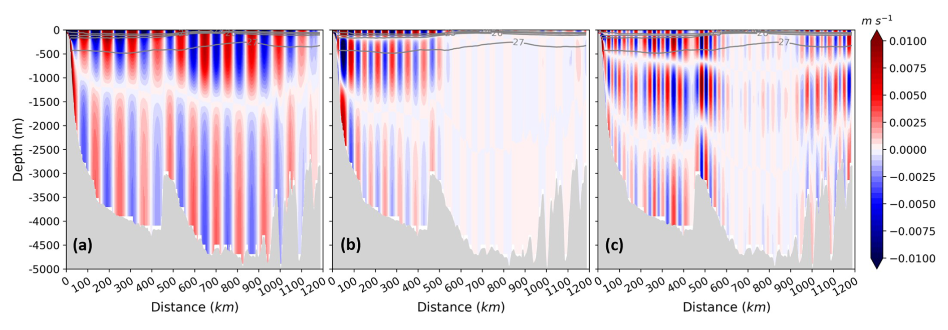
Figure B2 Vertical structure of the first three M₂ IT modes in the NE case. Snapshots (t= 6 h on 24 November 2015) of the along-transect baroclinic velocity component for modes 1 (a), 2 (b), and 3 (c) along the northeastward incident beam. All panels include selected mean potential density isopycnals (23–27 kg m⁻³, grey contours), and the seafloor topography (grey shading).

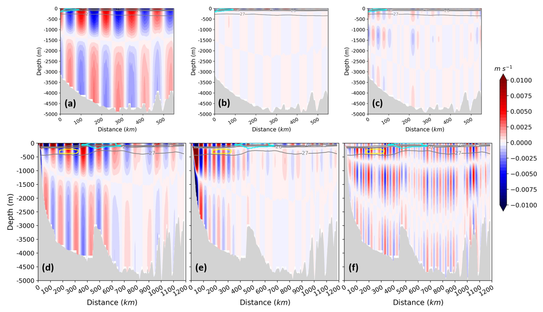
Figure B3 Vertical structure of the first three M₂ IT modes in the CEC case. Snapshots (t= 6 h on 17 September 2015) of the along-transect baroclinic velocity component for modes 1 (a, d), 2 (b, e), and 3 (c, f) along different beams: the northward refracted beam (a–c) and the northeastward incident beam (d–f). All panels include detected eddy edges for AE (yellow) and CE (cyan), selected mean potential density isopycnals (23–27 kg m⁻³, grey contours), and the seafloor topography (grey shading).

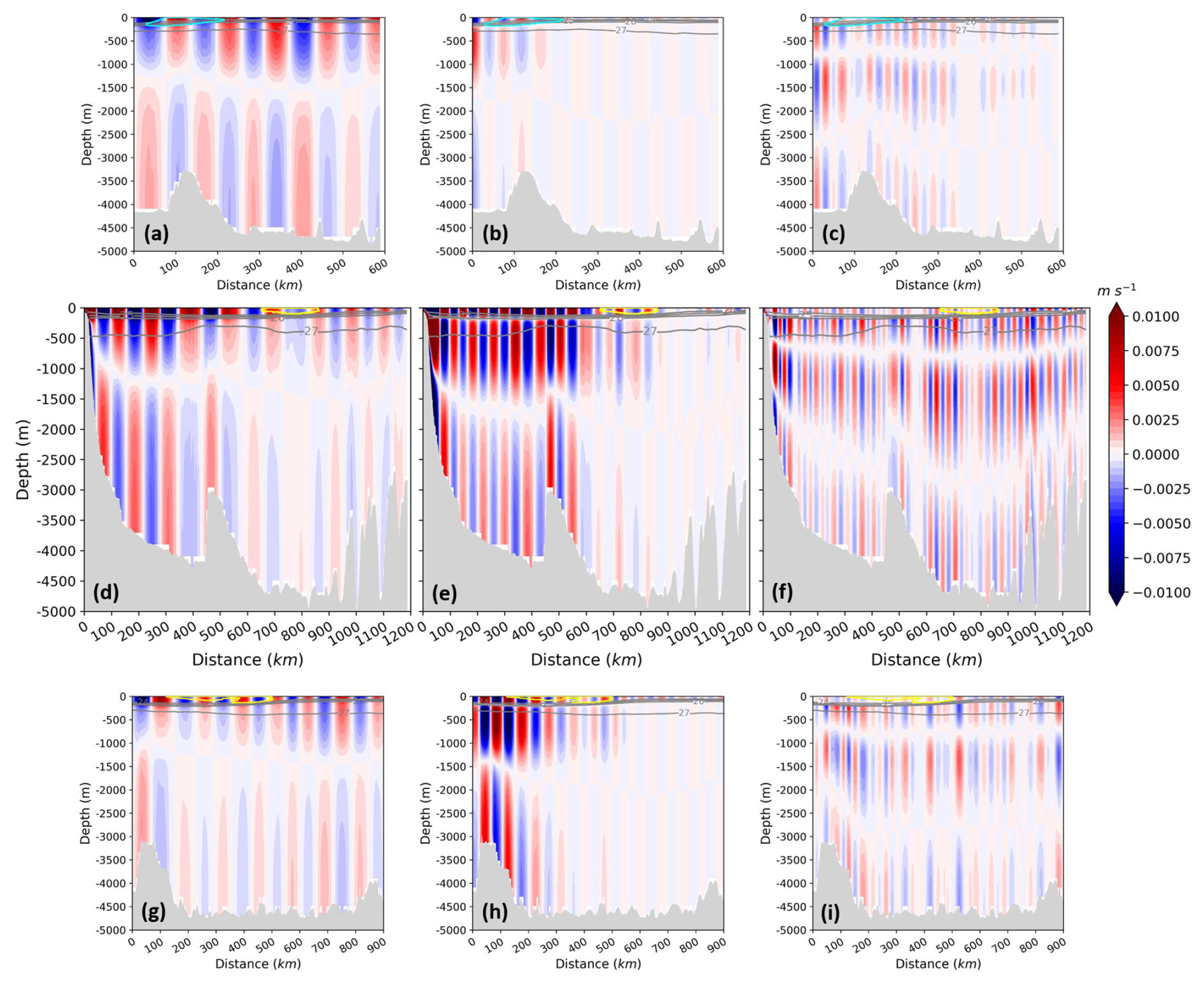
Figure B4 Vertical structure of the first three M₂ IT modes in the CEE case. Snapshots (t= 6 h on 29 September 2015) of the along-transect baroclinic velocity component for modes 1 (a, d, g), 2 (b, e, h), and 3 (c, f, i) along different beams: the northward diffracted beam (a–c), the northeastward incident beam (d–f), and the eastward diffracted beam (g–i). All panels include detected eddy edges for AE (yellow) and CE (cyan) eddies, selected mean potential density isopycnals (23–27 kg m⁻³, grey contours), and the seafloor topography (grey shading).