Seasonal impact of submesoscale eddies on the ocean heat budget near the sea ice edge

Oceanic submesoscale mixed layer eddies (SMLEs), with horizontal scales of 0.1–10 km, are not captured in climate models. SMLEs energized in the marginal ice zone (MIZ) have been shown to be of importance to sea ice melt rates in summer and to sea ice transport through notably a dynamical coupling with sea ice. Here our focus is on the thermodynamical coupling, which has received comparatively little attention. We aim to quantify, for the first time, the impact of eddies on both sea ice and the heat budget in the MIZ, contrasting different seasons and different background stratifications.

To this end, we set up SMLE-resolving simulations of the ocean mixed layer (ML) near the ice edge using the MITgcm, representing a lead or the MIZ. We isolate the effect of eddies by comparing 3D simulations with eddies to 2D (latitude-depth) simulations without eddies.

In summer (i.e., melting conditions) and regardless of the background stratification, SMLEs act as a heat pump from the atmosphere over the open ocean to the sea ice. On average over a season, SMLEs triple the meridional heat transport to the ice covered region, increase melting over their meridional extent, and trigger a positive radiative feedback by increasing shortwave absorption over the thinner ice. These changes are in the range 20 %–60 % for reasonable choices of shortwave forcing and initial ice thickness. In winter (i.e., freezing conditions), SMLEs have a relatively small impact on sea ice growth due to compensation between vertical and horizontal eddy heat transports. However, they reduce ML deepening by 80 %/50 % in the open/ice-covered ocean. Overall, our results reveal up to order one impacts of SMLEs on the heat and sea ice budgets in the MIZ, which will require the development of a SMLE parameterization tailored for polar regions.

1 Introduction

Sea ice is a critical component of the climate system, because of its high albedo and the way it mediates air-sea heat and momentum exchanges in polar regions. Predicting the evolution of the sea ice cover in both the Arctic and Antarctic is extremely challenging due to a lack of understanding of the climate processes influencing it (IPCC, 2023; Stroeve et al., 2012). Ocean heat content and transport have been shown to be a major regulator of the position of the sea ice edge as well as a leading driver of recent rapid Antarctic sea ice loss (Purich and Doddridge, 2023; Bitz et al., 2005; Aylmer et al., 2024, and references therein). This oceanic influence can be direct from the ocean to the sea ice but can also be mediated by air-sea exchanges near the ice edge (Aylmer et al., 2022). Aylmer et al. (2022) show, for instance, that increased ocean heat transport toward the Arctic is associated with increased heat release equatorward of the ice edge and increased atmospheric energy transport toward the central ice pack. As the Arctic sea ice cover is becoming more and more dominated by the Marginal Ice Zone (MIZ) – the region that lies between pack ice and open ocean (Vichi, 2022; Rolph et al., 2020; Frew et al., 2025), it is likely that such ocean-atmosphere-sea ice interactions will become increasingly important in regulating the sea ice extent.

In particular, both the MIZ and leads (cracks in the sea ice cover) represent areas of strong lateral density gradients in the upper ocean due to spatial heterogeneity of buoyancy forcing to the ocean. These upper ocean fronts lead, through baroclinic instability, to the energisation of submesoscale eddies (Haine and Marshall, 1998; Fox-Kemper et al., 2008; Swart et al., 2020; Horvat et al., 2016; Manucharyan and Thompson, 2017). While a handful of spottings from space in the 1960s first revealed their existence, modern observations and high-resolution modelling suggest that these submesoscale mixed layer eddies (SMLEs) are ubiquitous in the world ocean (Munk et al., 2000). SMLEs typically have length scales of the order of 100 m to 10 km, and time scales of days to weeks, i.e., Rossby number of order 1. Because of the weak stratification of the ocean mixed layer (ML), they are also associated with Richardson numbers of order 1. The importance of SMLEs cascades to the large-scale due to their influence on stratification, ML depth (MLD), air-sea interactions, and biogeochemical processes (Hewitt et al., 2022; Hosegood et al., 2006; Fox-Kemper et al., 2011; Thompson et al., 2016; McWilliams, 2016; Taylor and Thompson, 2023; Mahadevan, 2016).

In the last decade or so, submesoscale dynamics in polar regions has received increasing attention. Observational campaigns revealed the presence of submesoscale fronts and flows in abundance in polar regions (Timmermans et al., 2012; Timmermans and Winsor, 2013; Giddy et al., 2021; Swart et al., 2020). They also provided evidence for the impact of the sea ice cover on SMLE dynamics, for example by modulating the interaction with surface winds over the seasonal cycle (Giddy et al., 2021; Swart et al., 2020).

SMLE-sea ice interaction mechanisms have been further investigated in numerical modelling studies, though the emphasis has been largely on mechanical interactions. SMLEs, if energised in the MIZ, could mechanically trap sea ice floes and advect them into warmer waters, resulting in increased ice melt (Manucharyan and Thompson, 2017) although this effect is significantly modulated when thermodynamic interactions are also included (Gupta and Thompson, 2022). In leads and partially sea ice-covered regions, the ocean-ice friction could influence SMLE development. However, studies find somewhat contrasting results: while it was suggested that ocean-ice friction could reduce eddy overturning by 40 %, other studies showed that the influence of friction on eddy development is limited (Cohanim et al., 2021; Shrestha and Manucharyan, 2022; Brenner et al., 2023).

Horvat et al. (2016) and Horvat and Tziperman (2018) focused on thermodynamic interactions to show that, during the melting season, SMLEs have the potential to alter lateral melt rates by laterally transporting heat under ice. This process extends the dependence of floe melt rates on floe size up to 50 km – a much larger scale than previously thought when not considering SMLEs.

However, the thermodynamic interactions of SMLEs with sea ice cover and atmosphere remain under-explored. Observations and numerical modelling (e.g. Gupta and Thompson, 2022; Swart et al., 2020) suggest that the impacts of SMLEs should depend on the background oceanic and atmospheric conditions, and therefore should vary seasonally and regionally. For example, the impact of SMLEs on the polar environment is expected to differ between Arctic and Antarctic as the latter tends to exhibit a weaker upper ocean stratification than the former.

SMLEs are not resolved in global climate models, which rely on parameterizations. As the width of the Arctic MIZ increases under global warming, the importance of SMLEs in polar regions is expected to grow (Manucharyan and Thompson, 2022). Robust parameterizations of SMLEs in polar regions requires first solid understanding of their impacts, and then potentially, adaptations of parameterizations to polar conditions.

In the present study, we isolate the thermodynamic impacts of eddies in polar regions, which has been the focus of a limited number of previous studies (such as the afore-mentioned, Horvat et al., 2016; Horvat and Tziperman, 2018; Gupta and Thompson, 2022). Specifically, our aim is to understand the thermodynamic impact of SMLEs on sea ice, air-sea fluxes, and MLD in the vicinity of the sea ice edge (representing the MIZ or a lead). We expand on previous work by contrasting how the impact of SMLEs is modulated by seasons (sea ice growth versus melting conditions), background stratification (e.g., Arctic-like versus Antarctic-like temperature and salinity profiles), and MLD. To this end, we compare 3D submesoscale-resolving simulations with 2D (latitude-depth) simulations without eddies. This allows us to quantify eddy impacts through sea ice volume changes and heat budget terms, which we link to the eddy-induced overturning streamfunction (Fox-Kemper et al., 2008). We show that SMLEs have a leading order impact on the evolution of the ocean-ice state although the mechanisms are radically different between seasons. We also find that the background stratification is a key control in winter conditions but not in summer conditions.

The structure of the paper is as follows. In Sect. 2, the experimental set-up and the analysis methods are described. Section 3 gives the results, of which there are four subsections, Arctic summer (Sect. 3.1), Arctic winter (Sect. 3.2), sensitivity to background stratification (Sect. 3.3), and further sensitivity analysis (Sect. 3.4). The key results are summarised in Sect. 4, including the difference in eddy impact on sea ice, ML heat storage, air-sea flux and MLD depending on season and background stratification.

2 Materials and methods

2.1 Model set-up

In this study, the Massachusetts Institute of Technology general circulation model (MITgcm) is employed in hydrostatic mode (Marshall et al., 1997b, a). The model set-up is based on that used by Horvat et al. (2016). The domain is a reentrant zonal channel on an f-plane and is 75 km in both horizontal directions with walls on the northern and southern boundaries (Fig. 1a). A thermodynamic sea ice package is used, and there is no wind forcing. More details of the model set-up are provided in Sect. A1.

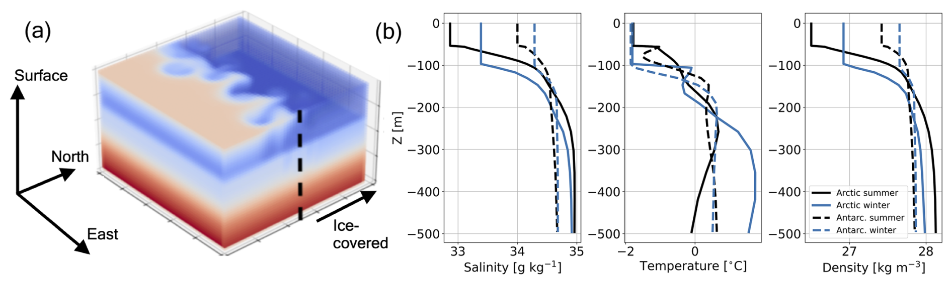
Figure 1 (a) Arctic summer set-up (temperature field), where the northern region is initially ice-covered and the southern region is ice-free. (b) Initial salinity, temperature and density profiles for Arctic/Antarctic-like stratification (solid/dashed lines) and for summer/winter (black/blue lines).

A 2-dimensional configuration (latitude-depth only), but otherwise identical to the 3D configuration is also set up. In this configuration, named “no eddies” hereafter, SMLEs are unable to develop because zonal variations and baroclinic instability are suppressed. Comparison between the 2D and 3D simulations provides measures of the impact of eddies (see Sect. 2.2).

The two main experiments represent summer and winter conditions with an Arctic-like initial stratification (we hereon refer to these two experiments as the Arctic summer and Arctic winter experiments, see Sects. 3.1 and 3.2). Furthermore, to test the sensitivity to background stratification, two summer/winter experiments are carried out using Antarctic-like initial temperature and salinity profiles (Sect. 3.3). The initial temperature and salinity profiles for these four experiments are taken from the EN4.2.1 ocean dataset (Good et al., 2013) near the ice edge. Specifically, for the Arctic, profiles were taken at (84° N, 0° E) in July and (83° N, 0° E) in January in 2016. For the Antarctic, profiles were taken at (63° S, 0° E) in July and (69° S, 0° E) in January. The ML temperature in all initial profiles is set to freezing point and for the winter/summer the initial MLD is 100/55 m. Sensitivity analysis to these initial MLD values is discussed in Sect. 3.4. The initial temperature and salinity profiles are shown in Fig. 1 and are horizontally uniform over the whole domain.

The atmospheric forcings and initial MLD values are (loosely) based on the European Centre for Medium-Range Weather Forecasts' atmospheric reanalysis version 5 (ERA5) and ocean reanalysis system 5 (ORAS5) near the ice edge at 0° E in 2016 (Hersbach et al., 2020; Zuo et al., 2019). For the summer experiments, the atmospheric temperature T_a is prescribed at −10 °C. Uniform downwelling shortwave forcing (F_SW,d) of 210 W m⁻² and downwelling longwave forcing (F_LW,d) of 220 W m⁻² are applied at the ocean surface. For the winter experiments, we use $T_{\mathrm{a}}=-\mathrm{5}$ °C, $F_{\text{SW},\mathrm{d}}=\mathrm{50}$ W m⁻², and $F_{\text{LW},\mathrm{d}}=\mathrm{175}$ W m⁻², which can be considered gentle winter conditions.

We emphasize that the initial conditions and surface forcings are not meant to capture specific observed conditions, but rather to test the sensitivity of SMLEs to typical conditions found in the Arctic/Antarctic MIZs in winter/summer times.

From the prescribed atmospheric conditions, the net surface heat flux, Q_net, is thus given (for the open ocean) by:

$$\begin{array}{}\text{(1)}& Q_{\text{net}}=F_{\text{LW},\mathrm{d}}-{\mathit{ϵ}}_{\mathrm{o}}\mathit{\sigma }{T}^{\mathrm{4}}+F_{\text{SH}}+(\mathrm{1}-{\mathit{\alpha }}_{\mathrm{o}})F_{\text{SW},\mathrm{d}},\end{array}$$

where F_LW,d is the downwelling longwave radiation, ϵ_oσT⁴ is the outgoing longwave radiation, ϵ_o is the ocean emissivity, σ is the Stefan-Boltzmann constant, and the net longwave radiation $F_{\text{LWnet}}=F_{\text{LW},\mathrm{d}}-{\mathit{ϵ}}_{\mathrm{o}}\mathit{\sigma }{T}^{\mathrm{4}}$. F_SH is the sensible turbulent heat flux, α_o is the ocean albedo and $F_{\text{SWnet}}=(\mathrm{1}-{\mathit{\alpha }}_{\mathrm{o}})F_{\text{SW},\mathrm{d}}$ is the net shortwave radiation absorbed by the ocean.

For the ice-covered ocean, the surface heat flux is computed using the 3-layer sea ice model of Winton (2000) (see also Sect. 8.6.1.1.3 of MITgcm contributors, 2026), in which the energy balance at the ocean/ice interface is between the conductive heat flux through ice, the shortwave penetration through ice and the latent heat of melting/freezing. As in the open ocean, we will use F_SWnet to denote the net shortwave radiation into the ocean.

All simulations are run for 110 d to roughly match the length of the season. To allow instabilities to develop in the 3D model, the initial temperature was seeded with small-amplitude white noise between 0 and 0.05 °C, so that the mean initial temperature in the mixed layer is slightly (+0.025 °C) above freezing. Results were found to be insensitive to the magnitude of the noise (tests were carried out for noise ±0.0125–0.8 °C).

2.2 Residual-mean framework

To explore the SMLE dynamics, we adopt a residual-mean framework (e.g. Marshall and Radko, 2003). In essence, the framework captures that the total averaged transport within a density layer has two components (Marshall and Speer, 2012). First, there is the product of the averaged meridional velocity $\stackrel{\mathrm{‾}}{v}$ and averaged layer thickness (in metres) $\stackrel{\mathrm{‾}}{H_{\mathit{\rho }}}$, $\stackrel{\mathrm{‾}}{v}\stackrel{\mathrm{‾}}{H_{\mathit{\rho }}}$. The second component is the eddy component $\stackrel{\mathrm{‾}}{v^{\prime }{H}_{\mathit{\rho }}^{\prime }}$, where dashes represent the departures from the average. Overall, we have $\stackrel{\mathrm{‾}}{v{H}_{\mathit{\rho }}}=\stackrel{\mathrm{‾}}{v}\stackrel{\mathrm{‾}}{H_{\mathit{\rho }}}+\stackrel{\mathrm{‾}}{v^{\prime }{H}_{\mathit{\rho }}^{\prime }}$. That is, the total (residual-mean) transport carrying, say, temperature is the sum of a Eulerian mean flow contribution and an eddy-induced contribution.

In practice here, following Abernathey et al. (2011) and others, we will show meridional overturnings (in Sverdrups) in the latitudinal-depth plane for convenience. The averaging is thus a time and zonal-average in 3D (effectively time-average only in 2D) and eddies are departures from this average. The residual-mean overturning, ψ_iso(y,z), is obtained first, by computing the overturning in density coordinates and remapping it to height coordinates, where it can be readily compared to the Eulerian overturning, $\stackrel{\mathrm{‾}}{\mathit{\psi }}(y,z)$. The eddy induced overturning is then obtained as the difference between the residual-mean and the Eulerian overturnings, ${\mathit{\psi }}_{\text{eddy}}={\mathit{\psi }}_{\text{iso}}(y,z)-\stackrel{\mathrm{‾}}{\mathit{\psi }}(y,z)$. Comparison of overturnings components in simulations with and without eddies will shed light on the role of the SMLEs.

For details of how ψ_iso is calculated with MITgcm outputs, see Sect. A2. For the 2D simulations, the streamfunctions are calculated the same way as in the 3D simulations, and then scaled by a factor L_x so that their magnitudes can be compared to the 3D streamfunctions.

Finally, note that, because ψ_eddy contains a departure from the time-mean component of the total circulation in both 2D and 3D simulations, it is sometimes referred to hereon as the transient component of the circulation. In particular, here, ψ_eddy includes the drift of system away from the initial conditions. This (small) contribution, which does not represent SMLEs, is noticeable in some simulations (see below).

3 Results

In this section, the results are discussed first for the Arctic summer experiment, starting with a description of the SMLE development, then the eddy impact on air-sea fluxes and sea ice, before describing the role of the eddy dynamics. Secondly, the results for the Arctic winter experiment are described (Sect. 3.2). Sensitivity experiments to an Antarctic-like initial background stratification are discussed for summer and winter in Sect. 3.3. Finally, results of the sensitivity of the eddy impact to MLD, atmospheric forcings and initial sea ice thickness are presented in Sect. 3.4.

3.1 Arctic summer

3.1.1 Submesoscale eddy development near to the ice edge

In summer, the atmospheric forcing drives ice melt and freshwater input in the northern half of the domain, while the shortwave radiation warms the open ocean faster than the ice-covered ocean. The atmospheric forcing therefore generates a meridional density gradient in the ML. Within a few meters from the surface, the developing ML meridional density gradient is dominated by salinity as the released freshwater from ice melt is very buoyant (lighter water on the ice-covered ocean side; Fig. 2a). However, below this freshwater lens down to the bottom of the ML, the meridional density gradient is temperature-dominated, with relatively warm water in the open ocean and near freezing temperatures in the ice-covered ocean (Figs. 2a and 3a). The MLD is defined using the default MITgcm surface-referenced density criterion. As a consequence of the spreading of the melt freshwater lens near the surface, the MLD rapidly drops to a few metres in just a few days in both ice-free and ice-covered areas, though the ML remains weakly stratified below this (Fig. 3c).

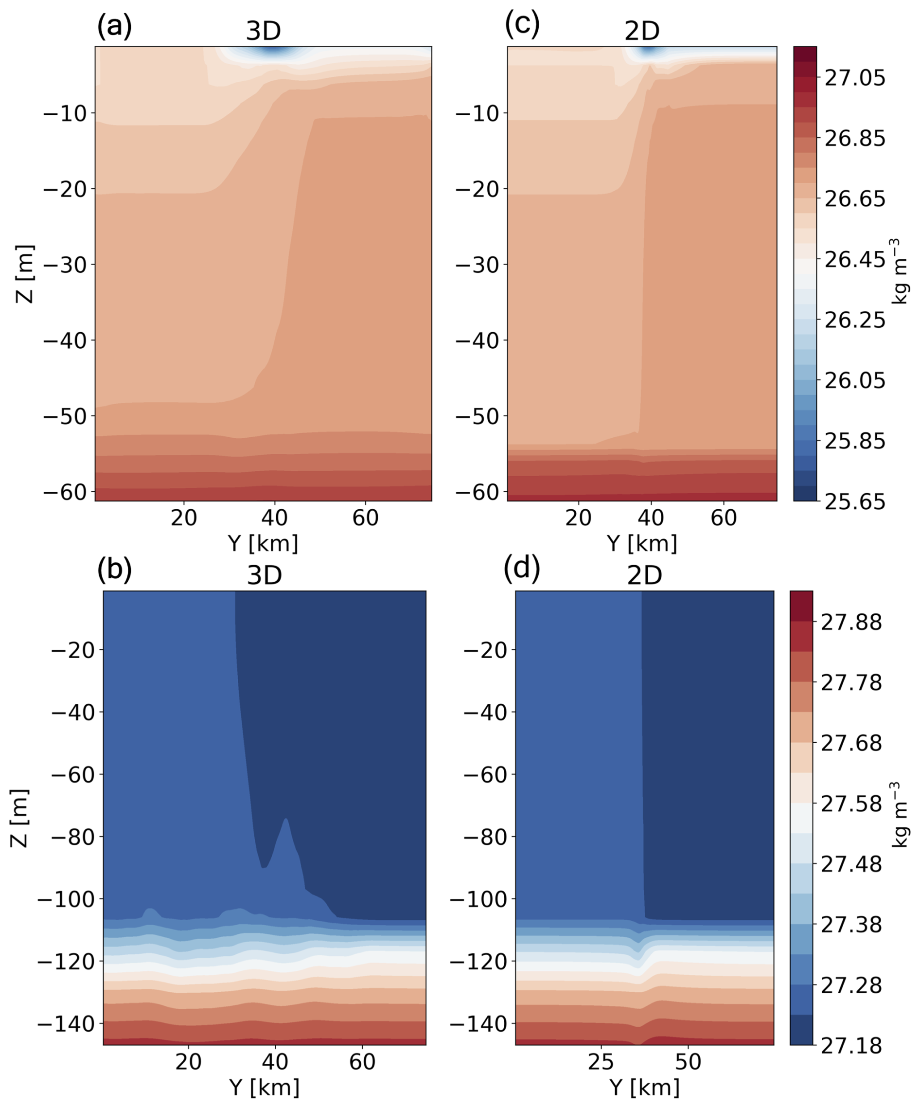
Figure 2 (a, c) Arctic summer and (b, d) and Arctic winter. Snapshots of potential density (referenced at the surface) for the (a, b) 3D (zonal mean) and (c, d) 2D simulations at day 50.

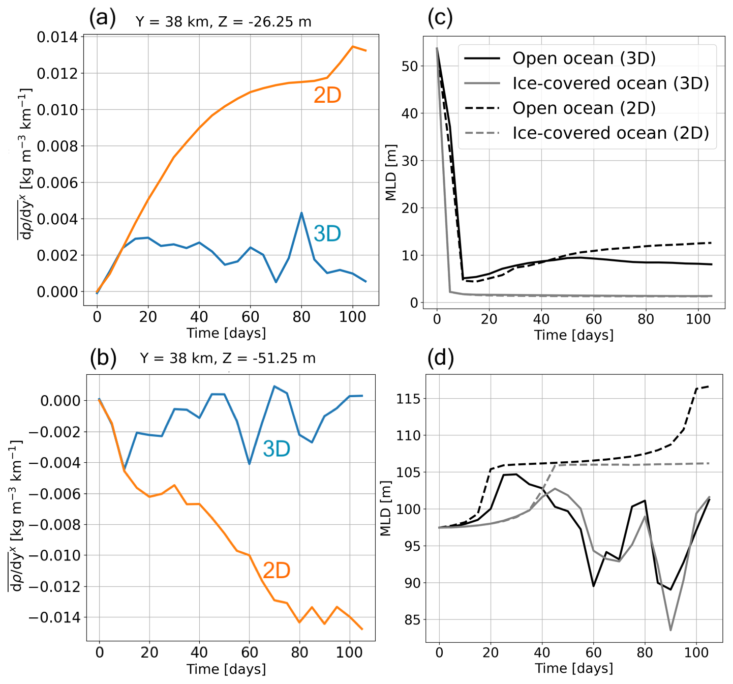
Figure 3 (a, c) Arctic summer, (b, d) Arctic winter. The left panels (a) and (b) display the time evolution of the zonally averaged meridional density gradient in 2D and 3D simulations at y=38 km, and $z=-\mathrm{26.25}$ m (summer) and z−51.25 m (winter). The right panels (c) and (d) display the time evolution of ice-covered and open ocean spatially averaged MLDs for 3D (solid lines) and 2D (dashed lines) simulations.

Through baroclinic instability, SMLEs develop near the ice edge, where the meridional density gradient is the strongest. Figure 4a displays the Rossby number, clearly highlighting the SMLE vortices that have been energised through the ML instability. The Rossby number is on the border of the submesoscale range at Ro≈0.3. By day 50, eddies are well developed, as illustrated by a snapshot of SST (Fig. 4c). The vertical eddy buoyancy flux ${\stackrel{\mathrm{‾}}{w^{\prime }{b}^{\prime }}}^x$ (where overline x is a zonal mean at constant height, prime denotes departure from the zonal mean, w is the vertical velocity, and $b=-g\mathit{\rho }/{\mathit{\rho }}_{\mathrm{0}}$ is the buoyancy) is shown at the surface and at depth $z=-\mathrm{28.75}$ m in Fig. 5a. A time average of ${\stackrel{\mathrm{‾}}{w^{\prime }{b}^{\prime }}}^x$ is shown in Fig. 5a (the time average is taken over the whole simulation period of 110 d). If the vertical eddy buoyancy flux is positive (bringing light water up or dense water down), then the eddies act to restratify the ocean ML. As described above, the meridional density gradient is dominated by salinity near the surface and temperature below the surface. Figure 5a illustrates that (1) eddies do not reach the full meridional extent of the domain by the end of the simulation in summer, (2) at the surface (salinity dominated) the vertical eddy buoyancy flux can be negative (i.e., destratifying), and (3) below a few meters, it is strictly positive (i.e. restratifying) with the strongest effect near the ice edge. It is noteworthy that the SMLEs extend over the full initial MLD of 55 m for the entire simulation despite the MLD dropping to a few meters within days (more details in Sect. 3.1.2). The weakly stratified ocean, from below the freshwater lens down to 55 m depth, remains prone to ML instability. The tendency of eddies to release available potential energy (PE), flatten isopycnals, and restratify the ML is therefore felt through the full depth of the initial ML. This is illustrated by comparing 2D and 3D density snapshots at day 50 (Fig. 2a and c). In the 2D run, the horizontal density gradient is more localised and stronger compared to that in the 3D run.

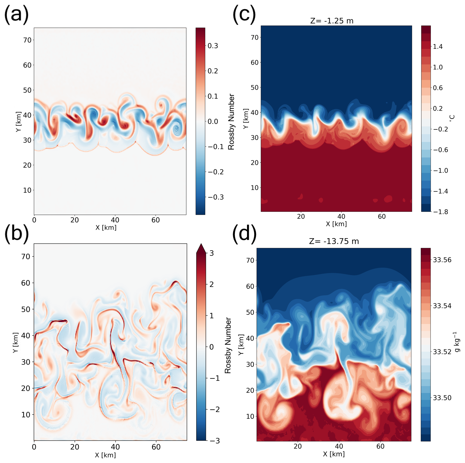
Figure 4 Snapshots of properties at day 50 for the Arctic case: (a, c) summer, (b, d) winter. Panels (a) and (b) display the Rossby number ($=\left|\mathit{\zeta }\right|/f$) at the surface (note the differing colourbars). Panel (c) displays the sea surface temperature, and panel (d) displays the salinity at a depth of $z=-\mathrm{13.75}$ m.

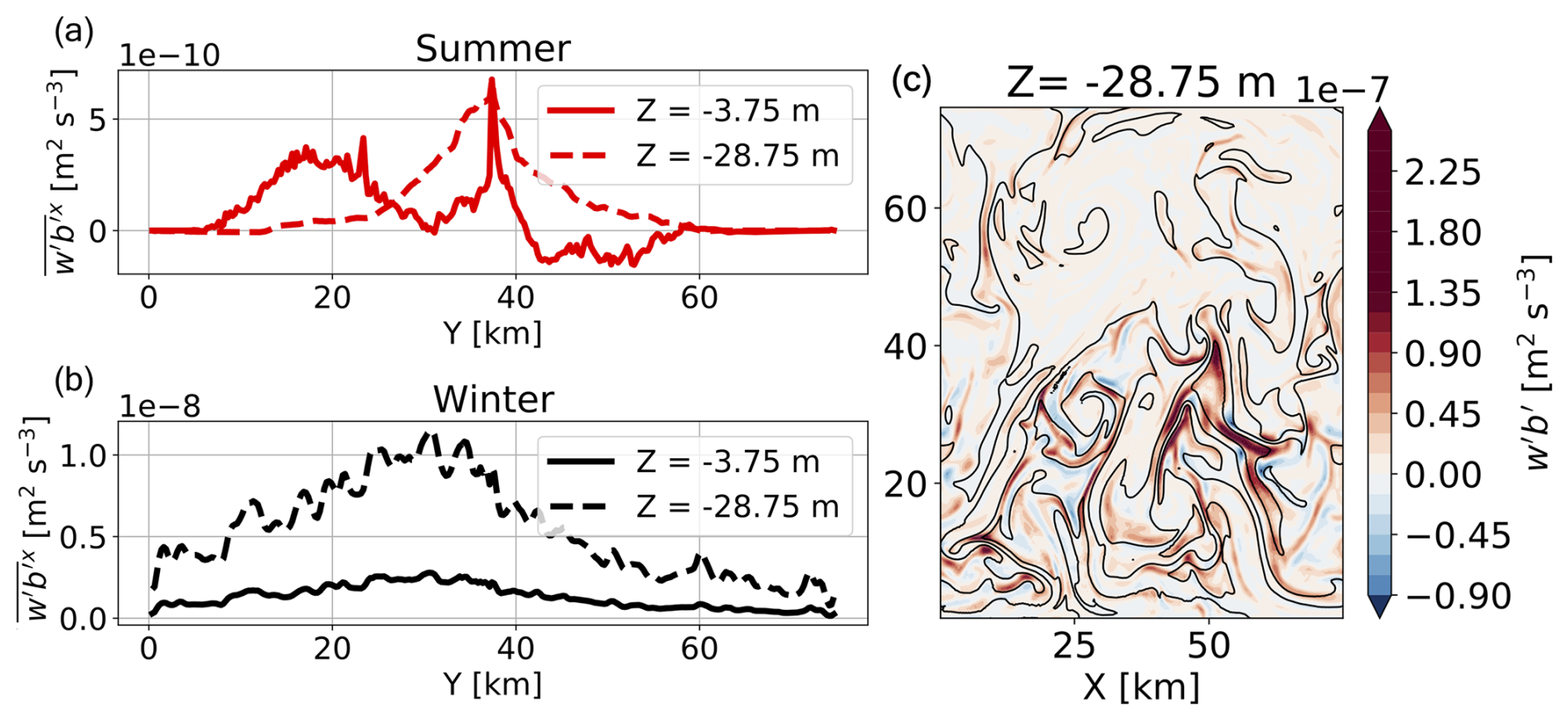
Figure 5 Time-averaged ${\stackrel{\mathrm{‾}}{w^{\prime }{b}^{\prime }}}^x$ at the surface and at $z=-\mathrm{28.75}$ m for (a) Arctic summer and (b) Arctic winter. Averages are taken over the full simulation length of 110 d. Note the different scales on the y axis between (a) and (b). (c) Spatial variations of $w^{\prime }{b}^{\prime }$ in the Arctic winter simulation at day 110, with salinity contours, spaced at 0.02 g kg⁻¹, shown in black.

3.1.2 Eddy impact on air-sea heat flux and sea ice

To evaluate the role of eddies, it is useful to explore the heat budget of the ML. We divide our domain into two boxes: an open ocean box from the southern solid wall to the middle of the channel (Y_b=38 km) and an ice-covered box north of Y_b=38 km. The two boxes extend from the ocean surface to a depth Z_b=55 m (the summer initial MLD). For each of these regions of volume V, the volume-averaged ML heat budget in units of W m⁻² is:

$$\begin{array}{}\text{(2)}& \begin{array}{rl}\underset{\text{storage}}{\underbrace{{\mathit{\rho }}_{\mathrm{0}}{c}_w{Z}_{\mathrm{b}}{\stackrel{\mathrm{‾}}{{\displaystyle \frac{\mathrm{d}T}{\mathrm{d}t}}}}^{xyz}}}& =\underset{\text{surface}}{\underbrace{{\stackrel{\mathrm{‾}}{Q_{\text{net}}}}^{xy}}}-\underset{\text{VHT}}{\underbrace{{\mathit{\rho }}_{\mathrm{0}}{c}_w{\stackrel{\mathrm{‾}}{wT|}}_{z=-Z_{\mathrm{b}}}^{xy}}}\\ & -\underset{\text{MHT}}{\underbrace{\left({\displaystyle \frac{{\mathit{\rho }}_{\mathrm{0}}{c}_w{Z}_{\mathrm{b}}}{Y_{\mathrm{b}}}}\right){\stackrel{\mathrm{‾}}{vT|}}_{y=Y_{\mathrm{b}}}^{xz}}}+F_{\text{diff}},\end{array}\end{array}$$

where $\mathrm{d}T/\mathrm{d}t$ is the temperature tendency, c_w is the heat capacity of seawater, and Q_net is the total surface ocean heat flux. Overlines denote spatial averages. The advective terms are the vertical heat transport (VHT) and the meridional heat transport (MHT). Because the box depth captures the vertical extent of SMLEs (being the initial MLD of 55 m in summer), the VHT across the box bottom is negligible. F_diff are the net diffusive heat fluxes into the box. Q_net is the net air-sea or ice-sea heat flux at the surface (see Sect. 2.1).

Under summer conditions, Q_net dominates the heat budget in the open ocean (Fig. 6a). Warming due to F_SWnet (𝒪(10²) W m⁻²) dominates. However, the atmospheric temperature of approximately −10 °C brings about sensible cooling of the ocean (𝒪(10¹) W m⁻²), which increases in magnitude over time (from around 30 to 50 W m⁻²) as the open ocean warms from (−1.8 to 3 °C). The increasing open ocean temperature also leads to a substantial increase in the magnitude of outgoing longwave radiation (−70 to −95 W m⁻²). Overall, steady warming due to F_SWnet (𝒪(10²) W m⁻²) is partially compensated by (an increasing) cooling by F_LWnet and F_SH, leading to a decrease of Q_net over time (Fig. 6a).

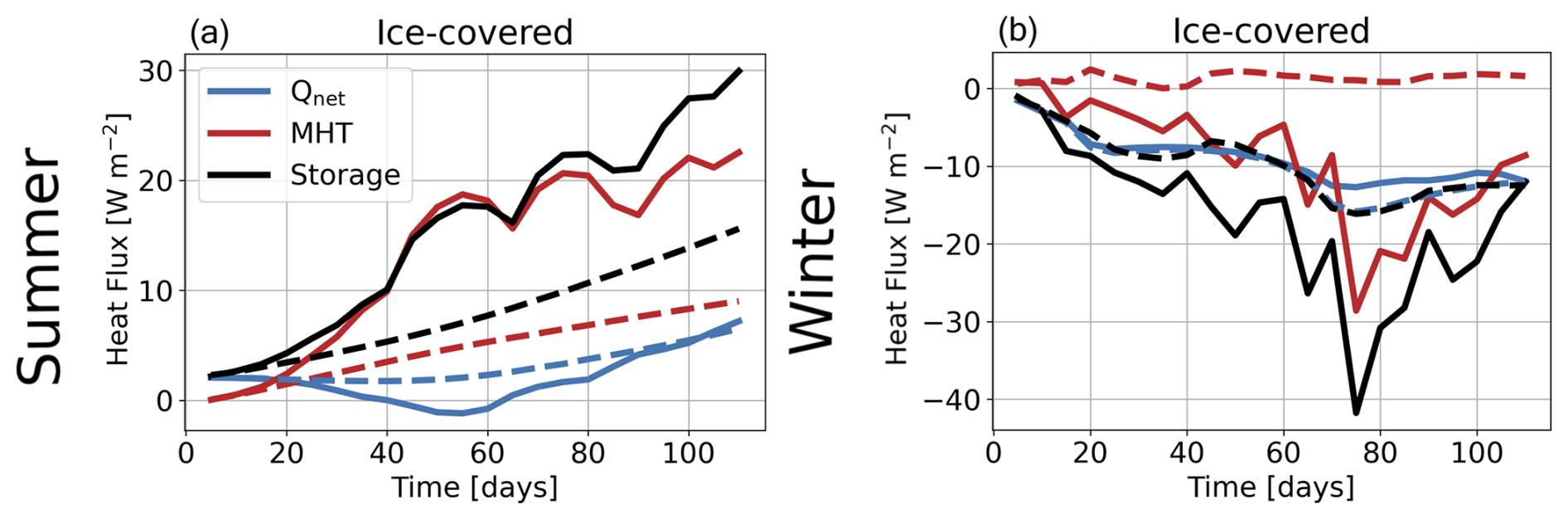
Figure 6 Top row: time evolution of Arctic summer open ocean (a) and ice-covered ocean (b) ML heat budgets. Bottom row: time evolution of Arctic winter open ocean (c) and ice-covered ocean (d) ML heat budgets. Solid and dashed lines denote the terms for the 3D and 2D simulations, respectively. For all quantities, 5 d averages are shown.

The open ocean heat storage is mainly driven by Q_net, but with a significant contribution from MHT (Fig. 6a). MHT (negative, pushing heat from the open ocean to the ice covered region) peaks at −35 W m⁻² in the 3D simulation, but only −9 W m⁻² in the 2D simulation. This MHT is almost entirely due to the eddy-induced overturning. Figure 7a shows that the total overturning, ψ_iso, is dominated by ψ_eddy. ψ_eddy is maximum underneath the initial ice edge and extends from below the freshwater lens down to 50 m depth. As expected, ψ_eddy (clockwise) flattens the density front, by lifting lighter water on the open ocean side and pushing down denser water under the ice (i.e., removing the available PE that feeds baroclinic instability). Since density gradients over most of the initial MLD are temperature dominated, ψ_eddy realizes a northward MHT into the ice-covered ML.

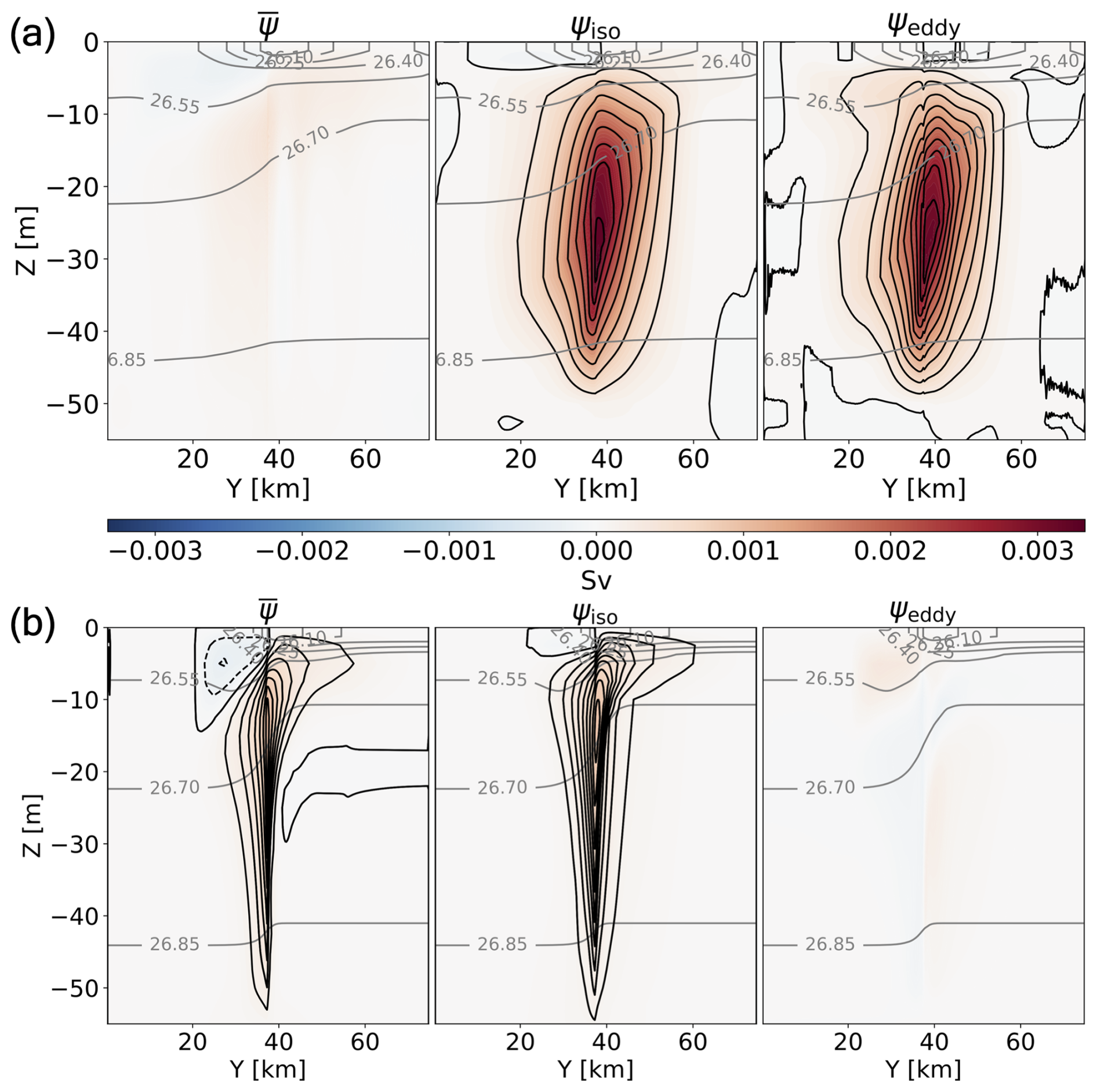
Figure 7 The Arctic summer time-averaged overturning streamfunctions for (a) 3D and (b) 2D simulations. $\stackrel{\mathrm{‾}}{\mathit{\psi }}$ (left panels), ψ_iso (centre panels), and ψ_eddy (right panels). Red/blue shadings indicate clockwise/counterclockwise cells. Time-averaged isopycnals are shown in grey. The time period of averaging is the full simulation length of 110 d.

VHT indicates a small exchange of heat between the ML and the deeper ocean (around 1 W m⁻² – not shown in Fig. 6). Vertical mixing terms were found to be negligible through the bottom boundary Z_b, and the surface correction term due to the linear free surface was also found to be negligible (not shown). Overall, the open ocean heat storage decreases by almost half over the 110 d (from 90 to 40 W m⁻²) as Q_net reduces over time and negative MHT strengthens in magnitude.

In the ice-covered ocean region (Fig. 6b), the net surface heat flux is almost 2 orders of magnitude smaller (only a few W m⁻²) than for the open ocean and changes little over time. All the heat flux components are much smaller in the ice-covered region than in the open ocean as expected, but there are also compensating effects. As the ice cover melts and thins (due primarily to heating from shortwave radiation), and the fraction of open water in this region increases, F_SWnet into this region increases by an order of magnitude to 𝒪(10¹) W m⁻², but cooling via longwave radiation and sensible heat flux also increases too. The resulting surface heating is balanced by ice melt, maintaining the ocean surface temperature at the freezing point (only slightly increasing due to the salinity-dependence of the freezing point). However, the storage term over the full initial MLD in the ice-covered ocean is overwhelmingly dominated by warming of the ML below a few meters, which is driven by the MHT from the open ocean region.

The impact of eddies on the heat budgets of both regions is observed by comparing the 3D and 2D results in Fig. 6a and b. In the ice-covered region heat budget, by day 110, the MHT in the 3D simulation is three times larger than in the 2D simulation, resulting in a storage twice as large in 3D than in 2D (compare red solid and dashed lines in Fig. 6b). This can be traced back to the radically different streamfunctions in 2D compared to 3D (Fig. 7). In 2D, there are no eddies and ψ_eddy is negligible (note that it is not exactly zero because of the transient component of the layer transport; see Sect. 2.2). Therefore, in contrast to the 3D case, ψ_iso is approximately equal to $\stackrel{\mathrm{‾}}{\mathit{\psi }}$. Interestingly, the latter is almost twice as large as in the 3D simulation, scaling with the stronger lateral density gradient in the 2D simulation. However, this is not enough to compensate for the negligible eddy-induced overturning, and overall the MHT from open ocean to ice-covered ocean is much larger with than without eddies.

This increased eddy-induced MHT to the ice-covered ocean supports a larger ice melt in 3D compared to 2D. The ice melt, in turn, impacts air-sea fluxes: a positive feedback is created between ice melt and F_SWnet as thinner and sparser ice coverage increases the fraction of ice-free ocean, and therefore the ML absorption of shortwave radiation (on average over the simulation, F_SWnet is increased by 20 % in 3D compared to 2D). There is a partial cancellation of this effect by increased cooling by longwave radiation and sensible heat flux for that fraction, but shortwave radiation dominates.

Comparing the time series of sea ice volume over the entire domain for 3D and 2D Arctic summer simulations shows the net large impact of the eddy heat transport on the ice cover (Fig. 8a). We scaled up the 2D time series by the number of zonal grid points in 3D for a meaningful comparison. The difference in total ice volume between the 2D and 3D simulations increases over time, reaching 10 % by day 110. This metric, however, underestimates the impact of SMLEs, which is concentrated within the meridional extent of the eddies. Figure 9 displays the sea ice volume at day 110 in 3D and 2D Arctic summer summed in the zonal direction. It emphasizes that the impact of SMLEs on sea ice is tightly linked to their spatial scale and growth rate. When only considering this region (bordered by the blue dotted lines), the final 2D-3D sea ice volume difference rises to 17 %. In Sect. 3.4, we also show that thinner initial ice cover leads to a much larger effect.

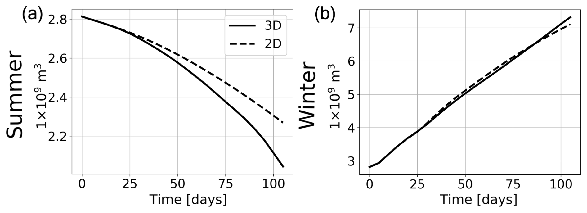
Figure 8 Total 3D (solid) and 2D (dashed) sea ice volume time series for (a) Arctic summer and (b) Arctic winter.

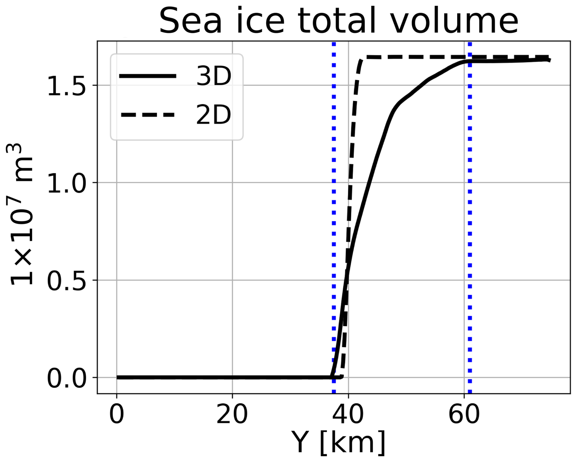
Figure 9 Day 110 snapshot of the zonal sum of sea ice volume, 2D and 3D Arctic summer (black lines). Blue dotted lines indicate the meridional extent of the eddies (underneath the ice cover).

3.2 Arctic winter

3.2.1 Submesoscale eddy development near the ice edge

Under winter atmospheric forcings, the ocean cools and ice forms within a few days. The rate of ice formation, which is associated with the rate of brine rejection, is faster in the open ocean, where ice is not already present or is thin. This is related to the conduction flux through ice which is inversely proportional to ice height. The salinity of the open ocean, therefore, increases faster than that of the ice-covered ocean (Fig. 4d). The developing winter ML density gradient (Fig. 3b) between the open and ice-covered regions is brought about by colder, saltier waters in the open ocean and warmer, fresher water in the ice-covered region (note that the density gradient is reversed compared to the summer case). That said, the gradient is salinity dominated as the ML is close to freezing point in both regions (the lateral temperature difference is less than 0.05 °C, compared to 3 °C in summer). This also implies that eddy buoyancy fluxes (Sect. 3.2.2) are not accompanied by significant lateral eddy heat fluxes in winter compared to summer. As a consequence of the surface buoyancy loss, the ML deepens and warmer water is entrained from below the ML (Fig. 3d).

SMLEs develop through ML baroclinic instability near the sea ice edge as in the summer. Compared to the summer simulation, eddies develop and spread more rapidly, as well as reach higher Rossby numbers (Fig. 4b). The eddies spread heat and salinity anomalies laterally (Fig. 4d), extracting the available PE from the lateral density gradient. As expected, the density front is steeper (Fig. 2, lower panels) and grows sharper (Fig. 3b) in 2D than in 3D.

The zonal-mean vertical eddy buoyancy flux ${\stackrel{\mathrm{‾}}{w^{\prime }{b}^{\prime }}}^x$ is an order of magnitude larger at depth ($z=-\mathrm{28.75}$ m) than at the surface (see Fig. 5b, where as in summer the time-averaged ${\stackrel{\mathrm{‾}}{w^{\prime }{b}^{\prime }}}^x$ is shown). At both depths, this restratifying flux is at least an order of magnitude greater than in summer (compare the y axis scale of Fig. 5a and Fig. 5b). This restratification (positive flux) by eddies opposes the destratifying influence of cooling and ice formation. In Fig. 5c, a snapshot of the winter spatial variations $w^{\prime }{b}^{\prime }$ are shown at day 110, with salinity contours shown in black. The alignment of $w^{\prime }{b}^{\prime }$ and salinity demonstrates that buoyancy anomalies are salinity dominated. $w^{\prime }{b}^{\prime }$ reaches up to 10⁻⁷ m² s⁻³ in parts of the open ocean, where air-sea fluxes are also larger. These magnitudes of vertical eddy buoyancy fluxes are equivalent to vertical heat fluxes (W m⁻²) in the submesoscale range (Fox-Kemper et al., 2011; Fox-Kemper and Ferrari, 2008; Thomas et al., 2008).

3.2.2 Eddy impact on air-sea heat flux and sea ice

As in the summer case, we investigate the heat budgets of the open ocean and ice-covered boxes. However, for the winter case, we set the bottom boundary of the boxes, Z_b, at the approximate final MLD of 147 m. This is to ensure that all the SMLE dynamics are included within the heat budget.

The rapid onset of ice cover in the open ocean has a large influence on the time evolution of the winter heat budget (Fig. 6c). All winter heat budget terms other than the net surface heat flux, the MHT and the heat storage, are negligible and are not displayed in Fig. 6. In the open ocean, the initial net air-sea flux is −77 W m⁻². It stays at this value throughout the simulation at locations that remain ice-free (because it is controlled by the SST, which remains at freezing point). Where ice grows, the surface heat flux decreases to approximately −10 W m⁻². This explains the initial rapid reduction of the net surface heat flux averaged over the initially open ocean from over −50 W m⁻² to around −30 W m⁻² (Fig. 6c). After around 40 d, Q_net is dominated by the presence of sea ice and changes little over the remaining 70 d of the simulation. The ice growth significantly affects all components of Q_net: F_LWnet (upwards) decreases from −120 to −82 W m⁻² (with a small effect due to decreasing SST), F_SH decreases from −7 to −3 W m⁻² and F_SWnet (downward) decreases by about one-half in 2D on average. As in the summer case, Q_net is the dominant term in the heat budget in the open ocean region although with weaker values (𝒪(10¹) W m⁻²).

The temperature tendency over the top few metres of the ML is actually close to zero, because of the balance between ice formation, heat lost at the surface, and heat entrained from below the initial MLD. As mentioned above, the depth-averaged lateral temperature gradient is weak (and reversed) compared to the summer case. As a result, the MHT acts to warm the open ocean, but it is smaller magnitude in winter than in summer.

In the ice-covered ocean region (Fig. 6d), the ice thickens over time in winter. Heat is conducted from the ocean through the ice and is lost to the atmosphere. Rates of ocean cooling (heat storage term) are lower than in the open ocean (by around 20 W m⁻²) due to a complete and thicker ice cover. The heat storage term is dominated by the net surface heat flux Q_net and MHT in 3D (both cooling the ice-covered box), and only by Q_net in 2D. Again, the volume-averaged heat storage term also encompasses heat mixed upwards and lost at the surface, through the process of deepening the ML.

The MHT at the initial ice edge (Y_b=38 km) is small in 2D, less than 1 W m⁻², but up to 17 W m⁻² in 3D. This difference mainly reflects the difference in the magnitudes of the total streamfunction ψ_iso between 2D and 3D (Fig. 10).

Figure 10 As in Fig. 7 but for Arctic winter. Note the different colorbar range compared to Fig. 7.

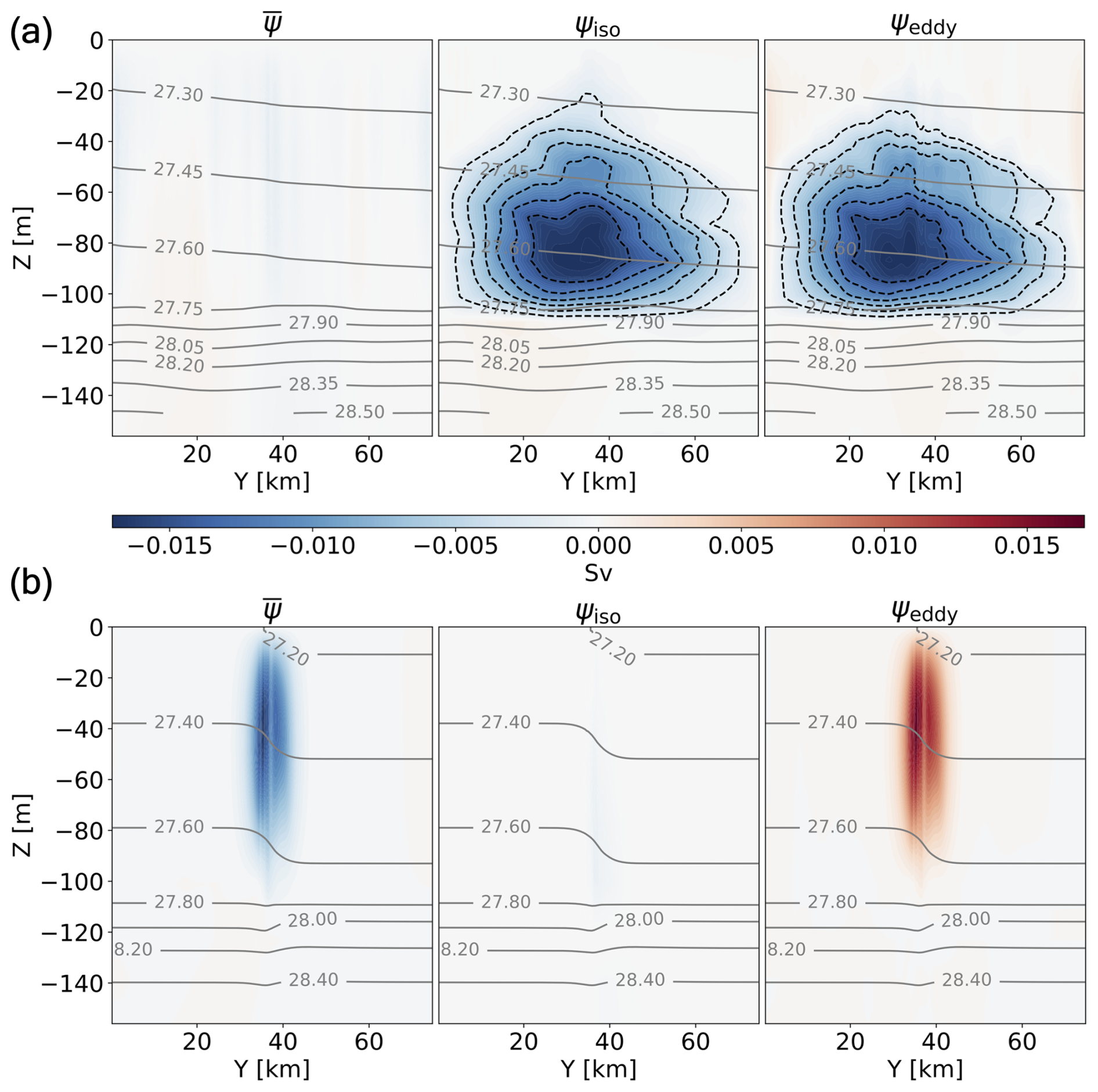
As in the summer simulation, the Eulerian streamfunction is negligible (Fig. 10a, left) and the winter total overturning is dominated by the eddy dynamics in 3D. The eddy-induced overturning is now anticlockwise (reflecting the reversal of the lateral density gradient between summer and winter). Eddies act to drive fresher, warmer water upward in the ice-covered region and cooler, saltier waters downward in the open ocean region.

In 2D, where SMLEs are absent, only temporal changes contribute to the eddy-induced overturning. Whilst in summer this transient contribution is negligible, in winter it is important when averaged over the entire simulation (but, again, by construction, it is zero when calculated instantaneously). ψ_eddy in 2D is clockwise with a narrow meridional extent. It is worth noting that, if this transient component exists in 3D, it would lead to an underestimation of the 3D eddy-induced overturning shown in Fig. 10a (right). Nevertheless, as in the summer simulation, the total overturning ψ_iso in 2D (no eddies) is an order of magnitude weaker than in 3D.

The southward eddy-driven MHT acts to partially compensate the heat loss to the atmosphere that drives ML deepening in the open ocean, hence reducing MLD deepening there (see Fig. 3d). The eddy-driven cooling of the ice-covered ocean has a significant impact on the heat budget, reinforcing the heat loss through ice. The ML average heat storage in the ice-covered region decreases further, by about 30 % on average over time, in 3D compared to 2D (Fig. 6d).

The overall effect of the eddies on sea ice growth is however small. Eddies increase the total ice volume (over the whole domain) by only 3 % by day 110. This is due to compensating effects. As more heat is transported laterally into the open ocean from under the ice in 3D than in 2D, less heat is obtained from below the ML in 3D, because eddies restratify and the ML does not deepen as much.

Figure 11 shows the time evolution of the difference in MLD between the 2D and 3D simulations (blue shading indicates deeper MLDs in 2D). The meridional expansion of the region with deeper 2D MLDs reflects eddies travelling further away from the initial ice edge over time. Eddies reduce the deepening of the ML by 80 % when averaged over the open ocean region and 52 % when averaged over the ice-covered region by day 110. The difference between regions is because cooling and ML deepening are more rapid in the 2D open ocean region than in the ice-covered one. In both regions, the final 3D MLD is only 5 m deeper than the initial one, implying that eddies nearly balance the destratifying impact of atmospheric cooling and ice formation in both regions.

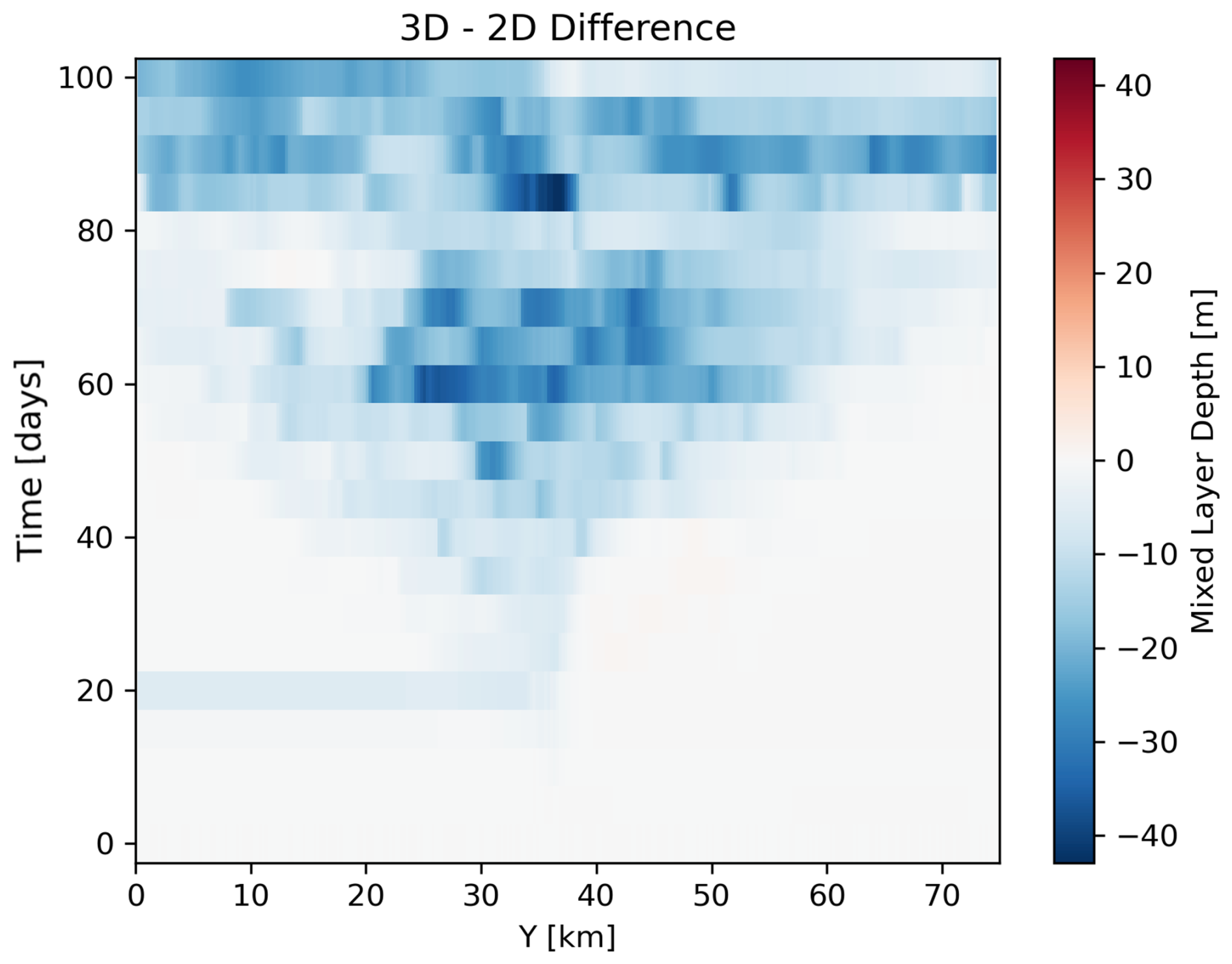
Figure 11 Time evolution of difference in MLD (zonally averaged) between simulations with eddies (3D) and no eddies (2D) for the Arctic winter case.

Nearer to the ice edge, the balance between these lateral and vertical heat exchange terms is very fine, but further south the difference is more stark and the differences between the 2D and 3D sea ice volume are larger. In the ice-covered region, rates of surface heat loss and also basal heating are a smaller factor in the heat budget, so lateral eddy heat transport is more important for heat storage and ice formation rates. This means there is also slightly higher ice growth and rates of heat loss in 3D compared to 2D in the winter ice-covered region. Overall, due to compensating eddy-induced MHT and VHT (though VHT in not displayed in Fig. 6, since the box captures full depth of SMLE dynamics), the rates of sea ice growth are not significantly impacted by the presence of eddies in the winter experiment.

3.3 Sensitivity to background stratification

This section explores the sensitivity of the SMLEs' impact to background stratification. To contrast with the stratification representative of the Arctic MIZ of the previous section, we use initial temperature and salinity profiles near the edge of the Antarctic sea ice cover, as described in Sect. 2.1 and Fig. 1.

3.3.1 Summer conditions

Under summer conditions, the Antarctic-like initial stratification results in only small differences in eddy impacts compared with the Arctic case. For example, eddies decrease the final ice volume by 11 % with Antarctic-like initial stratification, compared to 10 % in the Arctic case. The MHT to the ice-covered region is only 4 % larger for the Antarctic-like 3D simulation on average than for the Arctic case (Figs. 6b and 12a). The time-averaged open ocean heat storage, ice-covered ocean heat storage, and 3D ψ_iso exhibited negligible differences for the two differing initial background stratitications too. Therefore, eddies also have a significant impact on ice-covered region heat budget with this change in initial background stratification (Fig. 12a).

Figure 12 Ice-covered ocean ML heat budgets for (a) summer and (b) winter, (as in Fig. 6b and d but with initial Antarctic-like stratification rather than Arctic-like). As in Fig. 6, solid and dashed lines denote the 3D and 2D results with and without eddies, respectively.

This low sensitivity of the eddy impacts to initial stratification in the summer conditions is due to the tendency of the summer atmospheric forcings to enhance the upper ocean stratification and reduce the MLD abruptly. There is little interaction between the ML and the subsurface ocean in the summer simulations. Therefore, the differences in stratification deeper than the initial MLD do not alter the eddy dynamics and impacts.

3.3.2 Winter conditions

Unlike in the summer case, the sensitivity to background stratification is significant in winter. This is simply because the ML deepens under winter forcing. The rate of vertical mixing and the heat from the subsurface ocean that is mixed upward depend on the strength of the stratification, which is weaker in the Antarctic-like initial profiles than in the Arctic case. As a result, the rate of ML deepening with Antarctic profiles is significantly larger than with Arctic profiles (compare Fig. 13d with Fig. 3d). This also applies to the 2D case: rates of MLD deepening for the Antarctic-like stratification are over three times faster than in the Arctic (0.54 versus 0.16 m d⁻¹). However, the 2D-3D differences are similar with the two background stratifications, about 10–15 m. For reference, the final open ocean MLDs are approximately 160 m in 2D and 149 m in 3D for the Antarctic stratification compared to 118 m in 2D and 103 m in 3D for Arctic stratification. Using the 2D-3D difference in MLD as a proxy for the strength of eddy restratification, the effect is smaller in the ice-covered region than in the open ocean region with both stratification profiles. Note, however, that eddies stop and reverse the MLD deepening in the Arctic winter simulation, but can only slow down the ML deepening with the weaker Antarctic stratification.

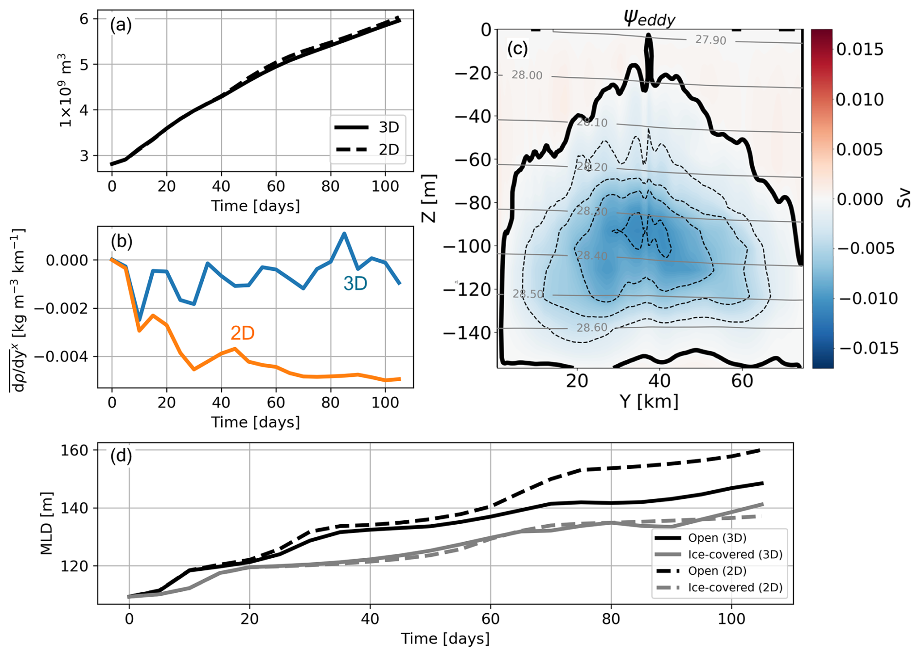
Figure 13 Results for the winter case with initial Antarctic-like stratification. (a) Time evolution of total sea ice volume for both 3D (solid line) and 2D (dashed line) simulations (compare with the Arctic case in Fig. 8b). (b) Time evolution of the zonally averaged meridional density gradient at y=38 km, and at $z=-\mathrm{51}$ m (compare with Fig. 3b). (c) The 3D eddy-induced overturning (compare with Fig. 10a, right panel). (d) Time series of MLDs for the open and ice-covered ocean (compare with Fig. 3d).

The greater vertical mixing of heat upwards from the subsurface ocean that occurs with the Antarctic stratification results in a slower ice formation, and in 2–3 times weaker lateral density gradients compared to the Arctic case (Figs. 13b and 3b). The 2D lateral density gradient reaches $\sim -\mathrm{0.005}$/−0.014 $\mathrm{kg}{\mathrm{m}}^{-\mathrm{3}}{\mathrm{km}}^{-\mathrm{1}}$ in the Antarctic/Arctic cases, respectively while the 3D gradients peak at $\sim -\mathrm{0.002}$ and $\sim -\mathrm{0.004}$ $\mathrm{kg}{\mathrm{m}}^{-\mathrm{3}}{\mathrm{km}}^{-\mathrm{1}}$ for the Antarctic/Arctic stratification, respectively. This effect can also be seen on the storage term in Fig. 12b, which is of greater magnitude with the Antarctic-like stratification than in the Arctic case. That said, it is worth to note that eddies have a small impact on sea ice cover in the winter simulations for both Antarctic-like and Arctic-like stratifications. By day 110, the 2D-3D difference in sea ice formation is −3 % for the Arctic case, whilst it is +3 % with the Antarctic-like stratification. Therefore, although there is faster MLD deepening and slower rates of ice formation overall (in both 3D and 2D) with the Antarctic-like stratification compared to the Arctic case, the eddy impact on sea ice formation (2D-3D difference) in winter is not altered by this change to the background stratification and remains small.

The eddy-induced overturning streamfunction with the initial Antarctic stratification is overall deeper (in line with a deeper MLD) but only slightly weaker than in the Arctic case (Fig. 13c). This is consistent with scalings from (Fox-Kemper et al., 2008), which predict a strengthening of the eddy-induced streamfunction with the MLD and the lateral density gradient. The weaker lateral density gradient and larger MLD in the Antarctic case might partially cancel out leaving an eddy-induced streamfunction of similar strength to that of the Arctic case. A more quantitative comparison of our results with the parameterization of Fox-Kemper et al. (2008) is left to a future study.

3.4 Sensitivity to MLD, atmospheric forcing, and initial sea ice thickness

Finally, in this section, we explore the sensitivity of the eddy impact to atmospheric forcing, the initial MLD, and the initial sea ice thickness. More specifically, we use the Arctic summer case with values of the prescribed downwelling shortwave radiation F_SW,d ranging from 180 to 270 W m⁻², of the initial MLD from 10 to 100 m, and of the initial sea ice thickness of 0.5 and 1 m. In addition, we investigate initial MLD values of 55 to 155 m for Arctic winter case.

Results of the sensitivity experiments are summarized in Fig. 14. There is a near monotonic increase of the 2D-3D difference of final total sea ice volume (in percent) with increasing F_SW,d (panel a) and initial MLD (panel b). The 2D-3D difference reaches 30 % for $F_{\text{SW},\mathrm{d}}=\mathrm{270}$ W m⁻² (due to stronger lateral density gradients and eddy MHT), and 14 % for MLD=100 m (again, due to stronger eddy overturning and associated MHT for deeper initial MLD).

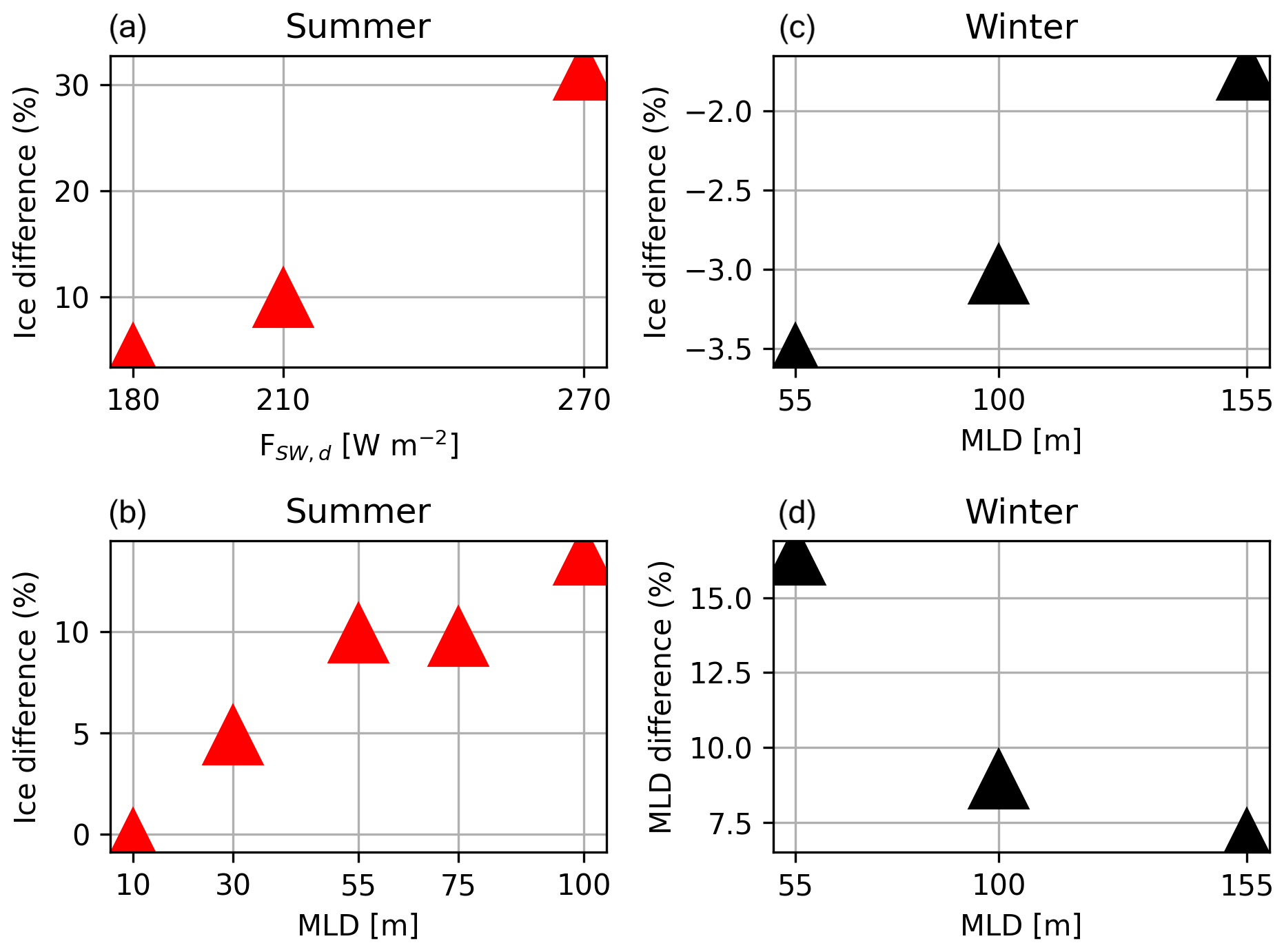
Figure 14 Sensitivity of Arctic summer 2D-3D ice volume difference to (a) F_SW,d and (b) initial MLD. Sensitivity of Arctic winter 2D-3D ice volume difference (c) and 2D-3D difference in the final MLD (d), to the initial MLD. All quantities are spatially averaged.

Furthermore, when the initial ice thickness in the Arctic summer simulation is decreased from 1 to 0.5 m, the 2D-3D percentage ice volume difference grows to 60 %. In absolute volume, the eddy-driven melt (as measured by the 2D-3D final ice volume difference) with 0.5 m initial ice height is around half that with 1 m initial thickness, but represents a much larger fraction of the initial thickness. Additionally, melt due to non-eddy effects (e.g., positive shortwave radiation feedback) is much greater over time with a thinner initial ice cover.

For the Arctic winter case, Fig. 14c displays the sensitivity of the eddy impact on ice formation to the initial MLD. Unlike the summer case, the impact of eddies on the total amount of ice formed is not sensitive to the initial MLD. The percentage ice difference varies between 1.7 %–3.5 % overall, effectively a doubling but this should be compared to a change from 0 % to 15 % in the summer case (panel b). Figure 14d shows how the percentage difference in MLD due to eddies decreases as initial MLD is increased – the figure ranges from 16 % with an initial MLD of 55 m to 7 % with an initial MLD of 155 m. This reflects how the eddies do not proportionally restratify the ML by the same fraction with increasing MLD. Instead, the absolute reduction to MLD by eddies is almost constant for all tested initial MLDs, 10 ± 1.5 m.

4 Summary and discussion

In this study, the impact of submesoscale mixed layer eddies (SMLEs) generated near the sea ice edge on the ocean, sea ice and air-sea exchanges is explored using idealized numerical simulations. Our focus is on the thermodynamical coupling between SMLEs and sea ice, which has received little attention in previous studies compared to mechanical coupling (hence we do not consider the wind forcing).

We use submesoscale-resolving simulations (at 250 m resolution) of the ocean mixed layer (ML) near the ice edge, representing a lead or the marginal ice zone. At the initial state, the northern half of the domain is covered with ice. 3D simulations with eddies are compared to 2D (no zonal variation, but otherwise identical) simulations where eddies are absent. To understand how SMLEs behave near the sea ice edge, we consider ambient conditions (the initial temperature and salinity profiles, atmospheric conditions) representative of the Arctic and Antarctic marginal ice zone, summer and winter conditions for both regions, different initial ML depths (MLDs), and different initial sea ice thicknesses.

The key outcomes of our study are:

• In summer, SMLEs energised near the ice edge have a leading order-to-moderate impact on air-sea heat exchange, ocean heat storage and lateral heat transport. Effectively, eddies act as a heat pump: taking heat out of the atmosphere to move it under the sea ice laterally, which in turn accelerates the melting of sea ice. The northward heat transfer is 3 times larger with than without eddies. This creates a positive feedback with an increase in shortwave absorption over the thinner ice. We estimate that eddies contribute a further decrease of the ice volume ranging from 10 % to 60 % depending on initial and boundary conditions.

• Under summer conditions, the above results are not significantly affected by the initial stratification. This is because the ML shallows rapidly and, therefore, the subsurface stratification does not influence the eddy development.

• In winter, we find a radically different situation. The direction of the eddy-induced overturning is opposite and at least an order of magnitude larger than in summer, with a faster pace of eddy growth and subsequent transport of density anomalies. This is consistent with an eddy growth rate proportional to the ML depth (MLD), which is larger in winter. However, the eddy-induced meridional heat transport is weaker than in summer because of the smaller meridional temperature gradient between regions (both at the freezing point).

• In winter, there are two competing eddy effects: with eddies, less heat is transferred upward into the ML from the subsurface ocean (ML deepening due to atmospheric forcing and ice formation is reduced, by about 10–15 m, with eddies due to their restratifying effects), but more heat is transported laterally by eddies from the ice-covered ocean. The former effect is marginally greater than the latter and so the net effect of eddies is to slightly increase ice growth in the open ocean region.

It is important to note that these findings may be limited by the simplifications of our model set-up. The simulations do not take into account the wind forcing. For example, a wind forcing would contribute to sustaining the MLD against the restratifying effect of the surface buoyancy forcing, effectively reducing the strong decoupling we observe between the ML and the subsurface in summer conditions. Other differences (such as sea ice characteristics, atmospheric forcing, and topographic constraints) could influence these results and enhance the differences between Arctic- and Antarctic-like experiments. Also, using a simple sea ice model (and our focus on thermodynamic interactions) implies that we did not consider processes such as dynamics of ice floes, which have been shown to interact strongly mechanically with SMLEs (e.g. Horvat et al., 2016; Gupta and Thompson, 2022). To move toward understanding of the real system, future work should aim to explore feedbacks between these effects. This may be particularly important for the improvement or design of submesoscale parameterizations for polar regions.

For the near future, including SMLEs in climate models will rely on effective parameterizations capturing key behaviors. SMLEs are important for polar regions as well as globally due to the way they regulate heat exchange between the atmosphere and the deeper ocean (Thompson et al., 2016). Including these eddies in climate models can have significant impacts on sea ice cover, global heat budgets, air-sea exchange, and nutrient transport (Su et al., 2018; Fox-Kemper et al., 2011; Mahadevan, 2016). In addition, capturing SMLEs can energise mesoscale eddies at the larger scale and global ocean currents such as the AMOC (Lévy et al., 2012; Fox-Kemper et al., 2011).

An intriguing finding of our study potentially relevant to parameterization is that the vertical scale of the eddies (and hence the eddy-induced circulation) is primarily set by the initial MLD. In summer in particular, as the ML shoals to 5 m within weeks, SMLEs retain the memory of the initial MLD (55 m) over 110 d. The eddies have little influence on MLD but still act to increase stratification over the full 55 m depth. In winter, the eddy-induced overturning extends slightly over time to match the final MLD (from 100 to 150 m for the experiment with Antarctic-like stratification). This suggests a significant decoupling from or lag (∼ month) of the eddy-induced overturning behind the MLD in summer. The Fox-Kemper SMLE parameterization (Fox-Kemper et al., 2008; Fox-Kemper and Ferrari, 2008; Fox-Kemper et al., 2011; Calvert et al., 2020) is currently the most used SMLE parameterization in climate models. Although this parameterization was not developed in the context of polar regions, it is regularly used in global set-ups, hence the need to evaluate its performance near the ice edge. On-going work explores the capabilities of the Fox-Kemper SMLE parameterization to capture the behaviour we have uncovered (to be published).

Overall, we have demonstrated that the thermodynamic SMLE-sea ice interaction leads to varying, up to leading order impacts of SMLEs on heat budgets, MLDs and sea ice cover of partially ice-covered regions. We have also shown that the impacts and mechanisms of SMLE impacts vary greatly with seasons. Finally, we have shown that the background conditions (stratification, sea ice thickness, forcing, MLD) can buffer or amplify these impacts.

Appendix A

A1 Model set-up

The horizontal grid spacing for the MITgcm set-up is 250 m and the vertical grid spacing is 2.5 m over the top 75 m. Below this, the vertical grid spacing increases by 20 % at each subsequent grid point to a total depth of 538 m. A thermodynamic sea ice package is used, such that the sea ice advection by the ocean is switched off. In addition, there is a free-slip boundary on the ice-ocean interface. The northern horizontal extent of the domain is initially covered with 1 m thick sea ice, and the southern half is open ocean. Further, there is no wind forcing. An atmospheric boundary model evolves the atmospheric temperature in response to air-sea/air-ice fluxes (Deremble et al., 2013). There is no evaporation or precipitation between ocean and atmosphere.

Vertical mixing is represented by the K-profile parameterization mixing scheme (Large et al., 1994). Under summer conditions, a Smagorinsky viscosity scheme is used, with the Smagorinsky scaling coefficient set to 2. In winter conditions, vertical mixing and vertical velocities are much more intense than in the summer due to the large surface buoyancy loss (e.g., sensible heat loss, brine rejection). This requires higher viscosity to maintain numerical stability. To avoid damping all motions, we employed a horizontal eddy viscosity of 50 m² s⁻¹ on the divergent component of the flow and of 1 m² s⁻¹ on the rotational component of the flow in the winter simulation. In addition, a small horizontal diffusivity of 1 m² s⁻¹ is also used in winter simulations. These values were selected (a higher horizontal viscosity on the divergent part of the flow $\partial v/\partial y$ and a lower viscosity on the rotational component of the flow $\partial u/\partial y$) to decrease grid-point noise, correlated to sea ice formation, on the meridional velocity field whilst not dampening the zonal jet. Sensitivity tests were conducted and these values were found to be the best for this purpose. To reduce the grid-point noise in the thermodynamic fields, the small amount of horizontal diffusion of temperature and salinity was introduced in the model. In addition, a third step to help with this issue was to change the smoothing settings within the KPP package. A few regularisations and smoothing options with the K-profile package were investigated. These include reducing the shear mixing when the velocity shear is low and the Richardson number is large. They helped to further reduce the noise in the velocity fields. In 3D we used the same values, whilst acknowledging this could potentially impact the development of SMLEs, by weakening the fronts.

A2 Calculation of the isopycnal streamfunction

The time-mean Eulerian overturning streamfunction is calculated via zonal integration at a fixed height of the meridional velocity field:

$$\begin{array}{}\text{(A1)}& \stackrel{\mathrm{‾}}{\mathit{\psi }}(y,z)=-L_x\underset{H_{\mathrm{d}}}{\overset{z}{\int }}\stackrel{\mathrm{‾}}{v}(y,z^{\prime })\mathrm{d}{z}^{\prime },\end{array}$$

where H_d indicates the ocean bottom, L_x is the zonal extent of the domain, and $\stackrel{\mathrm{‾}}{v}$ is the time and zonally-averaged meridional velocity field, which removes eddy effects.

Following Abernathey et al. (2011), the isopycnal streamfunction is defined as:

$$\begin{array}{}\text{(A2)}& {\mathit{\psi }}_{\text{iso}}(y,\mathit{\rho })=\underset{X}{\int }\underset{{\mathit{\rho }}_{\mathrm{d}}}{\overset{\mathit{\rho }}{\int }}\left(vh\right)\mathrm{d}{\mathit{\rho }}^{\prime }\mathrm{d}x,\end{array}$$

where $h=-\partial z/\partial \mathit{\rho }$ is a density layer thickness, ρ_d is the density of the deepest isopycnal, and ρ^′ is a dummy variable of integration.

Finally, the eddy-induced circulation ψ_eddy is obtained as the difference between $\stackrel{\mathrm{‾}}{\mathit{\psi }}$ and ψ_iso:

$$\begin{array}{}\text{(A3)}& {\mathit{\psi }}_{\text{eddy}}={\mathit{\psi }}_{\text{iso}}(y,z)-\stackrel{\mathrm{‾}}{\mathit{\psi }}(y,z).\end{array}$$

To calculate ψ_iso, the layers package in MITgcm is used. It calculates the layer transport $v{H}_{\mathit{\rho }}(x,y,\mathit{\rho },t)$ online (at every time step), where $H_{\mathit{\rho }}(x,y,\mathit{\rho },t)$ is the thickness of a density layer bin in metres (time averaging can be done later on). These density layer bins are chosen by the user at the start of the simulation. The full range of density bins chosen must cover the full range of ocean densities included in the simulation as well as their variation in time. ψ_iso(y,ρ) in Eq. (A2) is calculated by taking the cumulative sum of $\stackrel{\mathrm{‾}}{v{H}_{\mathit{\rho }}}(y,\mathit{\rho })$ (the sum was taken from the deepest isopycnal upwards). In this way, the meridional velocity v is integrated with respect to isopycnal layers rather than fixed vertical levels as in $\stackrel{\mathrm{‾}}{\mathit{\psi }}(y,z)$. Ideally, ψ_iso(y,ρ) should be robust to the choice of density bins used in its calculation. Here, ψ_iso(y,ρ) was found to be robust to the number of density layers when it is 92 or higher (tests were performed with 184 layers, and a 7 % or less L2 error was found for all four of the experiments).

ψ_iso(y,ρ) in Eq. (A2) is a function of density, not depth. Therefore it is convenient to remap it to height coordinates in order to compare it to $\stackrel{\mathrm{‾}}{\mathit{\psi }}$. Following the method of Wolfe and Cessi (2015), the remapping ${\mathit{\psi }}_{\text{iso}}(y,\mathit{\rho })={\mathit{\psi }}_{\text{iso}}[y,\stackrel{\mathrm{‾}}{\mathit{\rho }}(y,z\left)\right]$ is used. In practice, first, the cumulative sum of the time and zonally averaged layer thicknesses $\stackrel{\mathrm{‾}}{H_{\mathit{\rho }}}(y,\mathit{\rho })$ was taken, associating each density level with a single depth (which varies meridionally). This allows ψ_iso(y,ρ) to be interpolated from the meridionally varying heights $\stackrel{\mathrm{‾}}{H_{\mathit{\rho }}}(y,\mathit{\rho })$ to the fixed vertical grid.