Hidden vortices: near-equatorial low-oxygen extremes driven by high-baroclinic-mode vortices

Long-term time series of dissolved oxygen (DO) measurements from the upper 500 m of the eastern tropical North Atlantic (ETNA), collected over a period of up to 15 years at three different mooring sites, reveal recurring extreme low-oxygen events lasting for several weeks. Similarly, observations from 15 individual meridional ship sections between 6 and 12° N along 23° W show DO concentrations far below 60 µmol kg⁻¹ in the upper 200 m – significantly lower than the climatological values in this depth range (>80 µmol kg⁻¹). Two-third of these low-oxygen events could be related with high-baroclinic-mode vorticies (HBVs) with their cores located well below the mixed layer. Despite the energetic equatorial circulation and the expected dominance of wave-like structures in the near-equatorial region, these HBVs persist as relatively long-lived and coherent features. Based on moored and shipboard observations from the ETNA, and supported by an eddy-resolving ocean-biogeochemistry model, we characterize their dynamics and DO distribution. Observed water mass properties and model analyses suggest that most HBVs originate from the eastern boundary and can persist for more than six months. As they propagate westward into regions of higher potential vorticity (PV), anticyclonic HBVs with low-PV cores remain more effectively isolated and have longer lifespans compared to cyclonic HBVs with high-PV core. The vertical structure of the dominant anticyclonic HBVs corresponds to baroclinic modes 4–10, with associated Rossby radii ranging from 34 to 13 km, respectively. This is consistent with observed eddy sizes and is well below the corresponding 1st baroclinic Rossby radius of deformation (>100 km). Since none of the observed HBVs exhibit a surface signature, a substantial portion of the near-equatorial eddy field may remain undetected by satellites, yet still exert significant influence on local ocean ecosystems and biogeochemical cycles.

1 Introduction

Dissolved oxygen (DO) concentration is a key component of marine ecosystems, shaping biodiversity, biogeochemical cycles, and the survival of pelagic species (e.g. Deutsch et al., 2020). From long-term moored observations in the open Eastern Tropical North Atlantic (ETNA) near the equator (latitudes < 12° N), we repeatedly observe short-lived extreme low-oxygen events in the subsurface, well below the mixed layer. This DO variability is likely driven by small-scale vortices, which is unexpected, as theory suggests that wave-like structures should dominate at these latitudes (Eden, 2007). In this study, we combine moored time series, repeated ship transects, and an eddy-resolving biogeochemical model to investigate these small-scale processes below the mixed layer in the tropical Atlantic. This integrated approach allows us to characterize their structure, variability, and strong influence on DO distribution, with potential implications for marine ecosystems and biogeochemical cycles.

Extreme events of low DO in isolated cores of large coherent mesoscale eddies have become a well-studied phenomenon of the Atlantic and Pacific eastern boundary upwelling systems (e.g. Stramma et al., 2013; Karstensen et al., 2015; Schütte et al., 2016b; Frenger et al., 2018). A strong isolation and the longevity of such eddies over several months favor the existence of a DO depleted eddy core. The DO depleted core may result from (i) trapped water, which is transported westward within the eddy core from a region of initially low DO, typically from the eastern boundary (dynamic effect) and/or (ii) enhanced DO consumption (production effect) due to a biologically high productive regime above the eddy core (McGillicuddy, 2016). The latter is associated with high phytoplankton productivity, which leads to enhanced respiration and reduction of DO beneath the mixed layer directly in the isolated core reaching down to about 200 m (Karstensen et al., 2017). Respiration rates in the eddy's interior (at around 80 m depth) were found to be substantially increased, with up to 3 to 5 times the values of ambient conditions for the tropical North Atlantic (approximately 0.04–0.06 µmol kg⁻¹ d−1), e.g. subsurface intensified anticyclonic eddies (subsurface ACEs): 0.19±0.08 µmol kg⁻¹ d⁻¹ and surface intensified cyclonic eddies (CEs): 0.10±0.12 µmol kg⁻¹ d⁻¹ (Schütte et al., 2016b). The increased respiration within these isolated mesoscale eddies may result in anoxic conditions (<5 µmol kg⁻¹) in the otherwise hypoxic (>60 µmol kg⁻¹) ETNA. Such eddies can locally modulate biogeochemical processes and influence marine organisms (Fiedler et al., 2016; Hauss et al., 2016; Löscher et al., 2015). Moreover, it is suggested that the increased DO consumption within the isolated mesoscale eddy cores promote the formation and existence of a broad-scale shallow DO minimum zone (sOMZ) at about 80 m (Schütte et al., 2016b), that is most pronounced off the nutrient-rich Mauritanian upwelling system in the ETNA, located between 15 and 23° N (Karstensen et al., 2008; Brandt et al., 2015) (Fig. 1). For such low DO extremes to develop highly isolated eddies must form and propagate over a relatively long period through regions of relatively low dynamical activity, e.g. as stated in the mentioned literature north of 12° N in the eastern Atlantic and Pacific oceans.

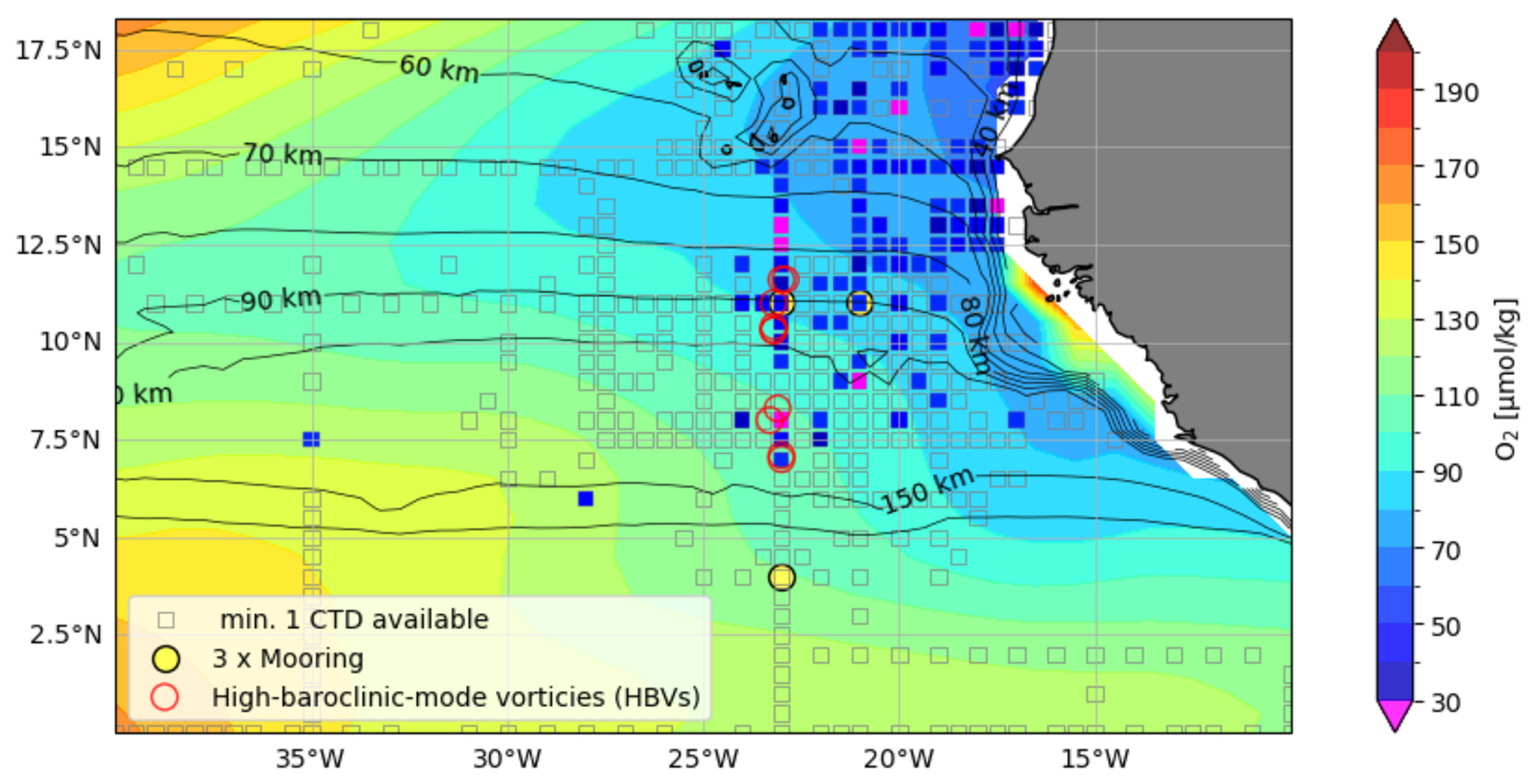
Figure 1 Map of the eastern tropical North Atlantic. Shaded are minimum dissolved oxygen (DO) values in the upper 200 m of the climatological DO distribution from the World Ocean Atlas 2023. The small squared boxes indicate regions of 0.5° boxes for which at least one CTD station is available. These boxes are colored with their minimum DO concentration in the upper 200 m (from multiple CTDs, if available) only if the minimum DO concentration is less than 60 µmol kg⁻¹. Red circles suggest the occurrence of high-baroclinic mode vorticies as analyzed in detail in the manuscript. The yellow points mark the positions of the moorings analyzed in the manuscript. The black contour indicates the first baroclinic Rossby radius of the deformation (in km), calculated from the World Ocean Atlas data, following Chelton et al. (1998).

The occurrence of DO depleted long-lived coherent eddies in near-equatorial waters (<12°) is not intuitive and contrasts theoretical considerations of equatorial dynamics, which suggest a dominance of anisotropic wave like structures (Eden, 2007). However, several extreme low DO events have been observed in the ETNA at latitudes between 6 and 12° N (Brandt et al. 2015), where Christiansen et al. (2018) associated one of these events (at 8° N, 23° W) with a subsurface ACE. These eddies are expected to be less isolated and shorter-lived compared to eddies poleward of these low latitudes. The first baroclinic Rossby radius of deformation (R_d,1), which is a characteristic threshold size of a dynamical regime to be in a geostrophic balance on meso- and larger scales, strongly increases towards the equator (Chelton et al., 1998). Global eddy studies, mainly based on altimeter sea surface height data, show a strong equatorward decrease of long-lived (>35 d) eddies (Chaigneau et al., 2009; Chelton et al., 2011). Less isolated eddies more readily entrain DO from surrounding waters, while short-lived eddies do not persist long enough to substantially deplete DO in their cores. Both factors inhibit the development of a low DO extreme within eddy cores. Additionally, the equatorial region – compared to the eastern parts of the oceans north of 12° N – is highly dynamic. It features the energetic equatorial zonal current system with associated instabilities as well as various wave phenomena (e.g. Urbano et al., 2006; Brandt et al., 2015; Peña-Izquierdo et al., 2015; Calil, 2023; Köhn et al., 2024). Nevertheless, our observations occasionally reveal DO values significantly below the climatological value (Fig. 1).

While mesoscale eddies of the first baroclinic mode can hardly exist at near-equatorial latitudes, smaller-scale eddies might. In the following, we refer to these smaller eddies, which still exhibit similar dynamics to mesoscale eddies - i.e., they are dominantly in geostrophic balance – as high-baroclinic mode vortices (HBVs). They have radii below the first baroclinic Rossby radius, R_d,1, and baroclinic modes larger than one (D'Asaro, 1988; McCoy et al., 2020; McWilliams, 1985). These HBVs, often referred to in the literature as subsurface or submesoscale coherent vortices, are observed to have isolated cores and can therefore advect tracers (Gula et al., 2019). Due to their small spatial scales and since they often appear at subsurface depth, these eddies are not necessarily detectable from satellite observations (McCoy et al., 2020). HBVs are not typically known to persist for extended durations in near-equatorial waters. However, here we provide evidence that HBVs may serve as a potential mechanism driving the observed low-oxygen extremes at these low latitudes. When linked to biogeochemical anomalies, HBVs may play a role in shaping local biogeochemical conditions and ecosystem variability. However, ocean models are often submesoscale “permitting” only, in the sense that the model has sufficient resolution to begin representing submesoscale processes but does not fully resolve them, particularly with increasing distance from the equator. Understanding the frequency and behavior of HBVs is essential for understanding tracer distributions, developing effective parameterizations and improving model accuracy.

In this study, we identify the characteristics, origin and temporal evolution of low-oxygen extremes in the upper 200 m of the tropical Atlantic Ocean and discuss the role of HBVs in driving these DO deficient zones. We use a comprehensive dataset of in situ moored and shipboard observations combined with an actively eddying ocean-biogeochemistry model (respective data and methods introduced in Sects. 2 and 3 in order to investigate the frequency distribution and magnitude of these events (Sect. 4.1). We show that the low-oxygen events are mostly associated with subsurface intensified HBVs (Sect. 4.2), both anticyclonic and cyclonic. We derive the demography of these structures from an eddy detection algorithm applied to in-situ observations (Sect. 4.3) and a vertical baroclinic mode analysis (Sect. 4.4). The core water of the HBVs is analysed in Sect. 4.5 and the origin and temporal evolution of the HBVs based in model simulations is shown in Sect. 4.6. We give a detailed discussion in Sect. 5 and provide a summary in Sect. 6.

2 Data

Data from moored, shipboard and satellite observations, climatological data as well as the output of an actively eddying ocean-biogeochemistry model from the tropical North Atlantic were used within this study as described in the following.

2.1 Moored observations

Multi-year moored observations from three different locations 11° N/21° W; 11° N/23° W and 4° N/23° W were used in this manuscript (Fig. 1). The mooring at 11° N/21° W was equipped with DO (AADI Aanderaa optodes of model types 3830 and 4330) and CTD (Conductivity, temperature, depth) sensors (Sea-Bird SBE37 microcats) which were attached next to each other on the mooring cable between 2012 to 2018. Eight of these optode/microcat combinations were installed evenly distributed in the depth range between 100 to 800 m, delivering multi-year time series of temperature, salinity and DO with a temporal resolution of up to 5 min. At 800 m depth, an upward looking Acoustic Doppler Current Profiler (ADCP) was installed to record velocity in the depth range between about 60 and 800 m. During the 2nd deployment period (May 2014 to September 2015), no velocity observations were available due to a failure of the ADCP. Before and after a deployment period, optodes and microcats were calibrated against CTD-O measurements during CTD casts and onboard lab measurements as described in Hahn et al. (2014, 2017). The correction against reference measurements, thereby considering potential sensor drifts (Bittig et al., 2018), allowed best data quality and yielded average root mean square calibration errors of 0.003 °C, 0.006 and 3 µmol kg⁻¹ for temperature, salinity and DO, respectively. Only quality controlled data that was flagged good was used for further analysis. ADCP measurements were quality controlled against a percent good criterion (20 % threshold) and were checked for plausibility and evident outliers due to surface reflection. ADCP bin depths were corrected using a mean sound speed profile following the approach by Shcherbina et al. (2005). This mooring is used to study hydrographic, DO and velocity temporal variability (on daily to intraseasonal time scales) related to low-oxygen extreme events. The other moorings at 11° N/23° W and 4° N/23° W are part of the prediction and research moored array in the tropical Atlantic (PIRATA), which were equipped with DO (AADI Aanderaa optodes of model types 3830 and 4330) sensors at 300 and 500 m depth from 2009 to 2024. At 11° N/23° W additionally a DO sensor at 80 m depth was installed between 2017 to 2024. The DO sensors deliver hourly data and are calibrated and processed in the same way as described above.

2.2 Shipboard observations

Hydrographic and DO data was obtained from CTD-O casts, that were carried out during a large number of research cruises to the tropical North Atlantic between 2006 and 2022. In the region 6–12° N and 30–18° W, 976 profiles were recorded during 24 cruises mainly covering the upper 1300 m of the water column. Two independently working systems of temperature-conductivity-pressure-oxygen sensors were used, that allowed to identify spurious sensor data. Salinity and DO readings were calibrated against values from water samples, that were taken during the majority of CTD-O profiles of each individual cruise and that were measured onboard with salinometry and Winkler titration, respectively. For a single cruise, data accuracy was generally better than 0.002 °C, 0.002 and 2 µmol kg for temperature, salinity and DO, respectively.

The majority of research cruises covered the 23° W meridian in the tropical North Atlantic. They captured several low-oxygen extreme events in the latitude range between 6 and 12° N (Fig. 1). We made use of these CTD-O observations that were mostly carried out at a meridional resolution of 0.5°, corresponding to 55 km, in order to investigate the spatial distribution of the low oxygen extremes. Horizontal velocity data were additionally acquired continuously along the cruise track with vessel-mounted Acoustic Doppler Current profilers (vmADCPs). The typical vmADCP operating frequency was 75 kHz, where 1 h averaged data has an accuracy of better than 2–4 cm s⁻¹ (Fischer et al., 2003). During one cruise, a vmADCP system with 150 kHz operating frequency was used and we expanded this data set with data from a lowered ADCP (lADCP), that was attached to the CTD rosette and measured velocity profiles at CTD-O cast positions. Single velocity profiles from lADCP had an accuracy of better than 5 cm s⁻¹ (Visbeck, 2002). The horizontal velocity observations from all 23° W ship sections covered the depth range of the upper 300 m, the depth where the extreme low-oxygen occur and thus coinciding with our target depth range.

For each 23° W ship section hydrography, DO and velocity were mapped onto a regular depth-latitude grid (resolution of 10 m and 0.05°) using a Gaussian interpolation scheme with vertical and horizontal influence (cutoff) radii of 10 m (20 m) and 0.05° (0.1°), respectively (for details see Brandt et al., 2010). This is done to plot the average section along 23° W in order to compare it with the model data and assess the model performance.

2.3 Satellite observations

Sea level anomaly (SLA) and surface geostrophic velocity derived from satellite altimetry products were used in this study to identify the surface signatures of eddies. The multimission Data Unification and Altimeter Combination System (DUACS) product in delayed time and daily resolution with all satellite missions available at a given time is used. It has a spatial resolution of 0.25° and is provided by Marine Copernicus (https://doi.org/10.48670/moi-00148).

2.4 Climatological data

Gridded climatological hydrography and DO from the World Ocean Atlas 2023 (WOA23) (described e.g. in Reagan et al., 2024) was used as a reference data set throughout this study. For more details see data availability section.

2.5 Coupled ocean–biogeochemistry model

We used the output of the GFDL climate model with an eddy-rich ocean, CM2.6 (Delworth et al., 2012; Griffies et al., 2015) to further understand the origin and development of low-oxygen extremes in the tropical ocean. CM2.6 has a nominal ocean resolution of 0.1° and an atmosphere with approximately 50 km resolution. For computational efficiency, marine biogeochemistry is represented by the simple biogeochemical model MiniBLING (Galbraith et al., 2015). MiniBLING was run with the three prognostic tracers dissolved inorganic carbon, phosphate and DO. Organic carbon (biomass) is treated diagnostically and is not advected in the model. Despite its simplicity, MiniBLING has been shown to perform comparably well to more complex marine biogeochemical models in simulating marine biogeochemistry and its sensitivity to climate (Galbraith et al., 2015). Moreover, the small number of tracers was not just a limitation but a key factor that made it possible to run a simulation with a mesoscale-rich ocean.

The results we show here stem from a simulation with preindustrial atmospheric carbon dioxide levels that has been run for 200 years, with marine biogeochemistry coupled at year 48. The model has been spun up from rest with initial conditions from WOA09 (Locarnini et al., 2010; Antonov et al., 2010; Garcia et al., 2010a, b) and Global Ocean Data Analysis Project (GLODAP) (Key et al., 2004). For more details on the model set up and a general evaluation of the model we refer to Griffies et al. (2015) and Dufour et al. (2015). Here, we used model output averaged over 5 d intervals for the last 20 years of the simulation. A brief evaluation of the model performance for the northern hemispheric Atlantic DO conditions, the focus of our study, is given in the following.

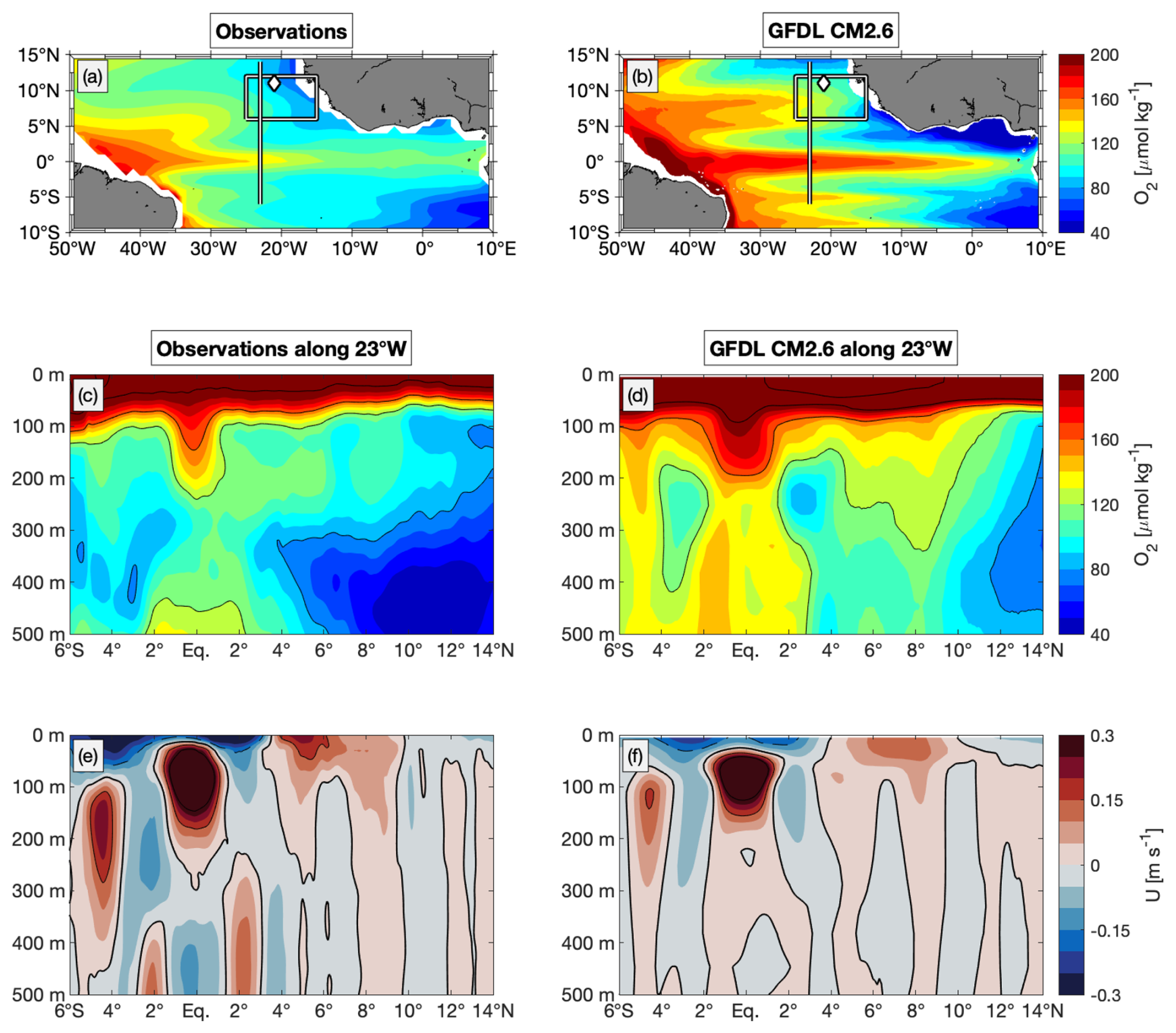
Figure 2 Observation-model comparison of the minimum DO between 0 and 200 m of the time-average distribution from (a) the World Ocean Atlas 2023 and (b) from last 20 years of GFDL CM2.6 model. Latitude-depth section, 0–500 m along 23° W, of mean DO from (c) repeat ship sections and (d) last 20 years of GFDL CM2.6 model. (e) and (f) are similar to (c) and (d), but mean zonal velocity is shown. The box in (a) and (b) illustrates the area of interest in this study; the line denotes the 23° W section that is shown in subpanels (c) to (f). This section has been surveyed by 15 individual shipboard observations that are used in this study for the latitude range 6–12° N. Diamond marks the mooring position (11° N/21° W), where data used in this study were taken.

The distribution of the minimum DO between 0 and 200 m taken from the time averaged over the last 20 years of the GFDL CM2.6 model output (Fig. 2b), shows similar large-scale patterns as the same corresponding distribution taken from the World Ocean Atlas 2023 climatology (Fig. 2a): well oxygenated western boundary region, decreasing DO values toward east with off-equatorial OMZs on both sides of the equator showing minimal values at the eastern boundary. The simulated distribution has higher DO concentration at the western boundary and in the interior basin, and partly lower values at the eastern boundary compared to the climatological distribution from observations, which is particularly the case in the Gulf of Guinea region. In the interior basin, meridionally alternating bands of oxygen-poor and oxygen-rich water, that are associated with shallow east- and westward current bands, are pronounced in GFDL CM2.6, albeit more intensified.

In the ETNA, the average DO distribution along 23° W in GFDL CM2.6 (Fig. 2d) shows a notable mismatch with observations (Fig. 2c). While observations from repeat ship sections reveal two distinct OMZ layers – a shallow OMZ above 200 m and a deeper OMZ at 300–700 m – the model instead simulates only a single OMZ spanning 100–600 m. This bias is also present in other coupled ocean circulation biogeochemistry models (e.g. Duteil et al., 2014) and can be attributed, among other factors, to the limited representation of physical transport processes such as submesoscale eddies, which locally enhance oxygen minima. Additionally, simplified or parameterized remineralization and biological processes fail to reproduce rapid upper-ocean oxygen consumption. These discrepancies highlight the importance of direct observational studies, such as ours, which provide detailed insights into the shallow oxygen minimum and its connection to low-oxygen events and high-baroclinic vortices, thereby motivating the focus of this study.

Further differences appear south of the equator, where the observed OMZ is absent in the model along 23° W. Instead, GFDL CM2.6 simulates lower DO levels between 2–4° N at depths below 150 m compared to observations. The corresponding section of zonal velocity (Fig. 2f) indicates that the model represents upper-ocean currents (above 200 m) well when compared to observations (Fig. 2e). However, below 200 m in the equatorial region (5° S–5° N), zonal currents are considerably weaker and partly misrepresented. North of 5° N, the velocity structure is generally better captured.

Despite differences in spatial details and magnitudes the basic features of the DO and velocitiy distributions are in the upper 200 m of the ETNA, and the GFDL CM2.6 model provides a robust physical and biogeochemical background state to study the role of eddies in driving local DO deficient zones. With a nominal ocean resolution of 0.1°, CM2.6 is mesoscale eddy-resolving and submesoscale-permitting at low latitudes, capturing only the larger submesoscale vortices. The local Rossby radius of deformation (60–150 km; Fig. 1) in the area is resolved, but smaller eddies are near the lower limit of resolvable scales. However, the model has been shown to simulate low-oxygen mesoscale eddies at latitudes poleward of about 12° latitude (Frenger et al., 2018) and provides as a useful framework in this study to complement the observational analysis. Here, we use the last 20 years of this model run to study low-oxygen extreme events in the ETNA equatorward of 12° N.

3 Methods

Different diagnostics have been applied in this study, that allowed us to associate low-oxygen features with HBVs and to analyze their origin and temporal evolution. The concept of vertical baroclinic modes (Sect. 3.1) was used to characterize the vertical structure of HBVs, to identify the dominant vertical modes, and their associated Rossby radius of deformation and propagation speed. In Sect. 3.2, we briefly present the calculation of PV, which is used as a conservative tracer to track and to identify the isolation of different water masses. In Sect. 3.3, we describe the different approaches for eddy identification from shipboard observations and in the GFDL CM2.6 model.

3.1 Vertical baroclinic modes and Rossby radius of deformation

A powerful way to describe linear wave dynamics in the ocean is the decomposition into vertical baroclinic modes (Philander, 1978). Each baroclinic mode is associated with a specific gravity wave speed and a corresponding Rossby radius of deformation, which defines its characteristic horizontal length scale.

3.1.1 Baroclinic mode decomposition

The concept of baroclinic modes is based on the linearized hydrostatic equations of motion, which can be separated into a horizontal and a vertical component. Assuming a motionless background state and a flat-bottomed ocean, the vertical structures are given by solving the eigenvalue problems (Gill, 1982):

$$\begin{array}{}\text{(1)}& {\displaystyle \frac{{\mathrm{d}}^{\mathrm{2}}{\mathrm{\Psi }}_n\left(z\right)}{\mathrm{d}{z}^{\mathrm{2}}}}+{\displaystyle \frac{N^{\mathrm{2}}\left(z\right)}{c_n^{\mathrm{2}}}}{\mathrm{\Psi }}_n\left(z\right)=\mathrm{0}\end{array}$$

where Ψ_n(z) describes the vertical structures of isopycnal displacement ξ or vertical velocity w and z is the vertical coordinate. N(z) is the vertical profile of the Brunt–Väisälä frequency and c_n the gravity wave speed for mode n∈N. For the eigenvalue problem (1), we use boundary conditions with a free surface and a flat bottom (Gill, 1982), which are given as

$$\begin{array}{}\text{(2)}& {\mathrm{\Psi }}_n={\displaystyle \frac{c_n^{\mathrm{2}}}{g}}{\displaystyle \frac{\mathrm{d}{\mathrm{\Psi }}_n}{\mathrm{d}z}},\mathrm{at}z=\mathrm{0}\mathrm{and}{\mathrm{\Psi }}_n=\mathrm{0},\mathrm{at}z=-H\end{array}$$

where H is the ocean depth and g the gravitational acceleration. For a continuously stratified ocean, the number of solutions depends on the vertical resolution of the data used. Any perturbances can be described as a superposition of orthogonal vertical baroclinic modes (n=1, 2, 3, …). Amplitudes of vertical structure functions are normalized such that

$$\underset{-H}{\overset{\mathrm{0}}{\int }}{\mathrm{\Psi }}_n{\mathrm{\Psi }}_m\mathrm{d}z={\mathit{\delta }}_{nm}H$$

where δ_nm is the Kronecker delta and nm the modes. The gravity wave speed is related to the Rossby radius of deformation, that can be calculated for the off-equatorial regions (poleward of 5° S and 5° N) as

$$\begin{array}{}\text{(3)}& R_{\mathrm{d},n}={\displaystyle \frac{c_n}{\left|f\right|}}\end{array}$$

(Gill, 1982 or Chelton et al., 1998), where R_d,n is the Rossby radius of deformation for the nth vertical baroclinic mode, and f is the Coriolis parameter.

3.1.2 Calculation of vertical baroclinic modes and modal decomposition

The main goal is to decompose any disturbed state into the set of orthogonal baroclinic modes that solve (1). Each hydrographic profile from an individual CTD-O profile can be considered as a perturbation from the mean state. The mean state distribution was derived from the 3D climatological hydrographic field (cf. Chelton et al., 1998) that is given by the World Ocean Atlas (Sect. 2.4). Given the corresponding density profile, we calculated the isopycnal displacement ξ(z) by

$$\begin{array}{}\text{(4)}& \mathit{\xi }\left(z\right)={\displaystyle \frac{{\mathit{\rho }}^{\prime }\left(z\right)\cdot g}{{\mathit{\rho }}_{\mathrm{0}}\cdot N^{\mathrm{2}}}}\end{array}$$

with ${\mathit{\rho }}^{\prime }\left(z\right)=\mathit{\rho }\left(z\right)-{\mathit{\rho }}_{\mathrm{ref}}\left(z\right)$, ρ₀=1025 kg m⁻³ a constant reference density and ρ_ref being the undisturbed profile of potential density (here taken as the climatological density profile from the World Ocean Atlas – see also Vic et al., 2021 for more details on the method used). The isopycnal displacement of the disturbed state can be described as a superposition of the orthogonal set of vertical baroclinic modes for displacement, i.e.

$$\begin{array}{}\text{(5)}& \mathit{\xi }\left(z\right)=\sum _{n=\mathrm{1}}^K{x}_n{\mathrm{\Psi }}_n\left(z\right).\end{array}$$

Here, K→∞ expresses the exact solution with an infinite number of vertical modes for a continuously stratified ocean. The expansion coefficients x_n are the modal amplitudes. The modal amplitudes are obtained by projecting the observed fields onto the structure functions computed from the World Ocean Atlas. The projection is preferred over resolving a least-square problem, which sometimes leads to unrealistic modal amplitudes into the high modes (Vic and Ferron, 2023). The modal amplitudes x_n are calculated via a scalar product:

$$\begin{array}{}\text{(6)}& x_n=\underset{-\mathrm{980}}{\overset{-\mathrm{30}}{\int }}{\mathit{\psi }}_n\left(z\right)\cdot {\mathit{\zeta }}_{\mathrm{CTD}}\left(z\right)\mathrm{d}z.\end{array}$$

These amplitudes are then normalized by dividing with $\underset{-\mathrm{980}}{\overset{-\mathrm{30}}{\int }}{\mathit{\psi }}_n(z{)}^{\mathrm{2}}\mathrm{d}z$. This analysis is restricted to the depth range from 30 to 980 m in order to exclude the surface mixed layer while retaining the majority of available profiles along 23° W. The barotropic mode assumed to be zero. A vertical resolution of 10 m is used, with both the CTD profiles and World Ocean Atlas data interpolated accordingly. After computing the contribution of one mode, it is subtracted from the displacement profile: ${\mathit{\xi }}^{\prime }\left(z\right)=\mathit{\xi }\left(z\right)-x_n{\mathrm{\Psi }}_n\left(z\right)$ and the procedure is repeated for the next mode. This recursive removal reduces cross-talk between modes caused by the limited vertical resolution and incomplete depth coverage. Since the order of mode extraction may influence the result, the decomposition is repeated M=100 times with random permutations of modes n=1 to n=20, and the final modal amplitudes are calculated as the mean over all realizations, with associated standard errors.

3.2 Potential vorticity and Rossby number

Subsurface eddies exhibit signatures of high or low potential vorticity (PV), depending on their stratification anomaly and rotation direction (D'Asaro, 1988; McWilliams, 1985; Molemaker et al., 2015). In the absence of mixing, PV is a conserved quantity and serves as an effective tracer to differentiate water masses and track eddy pathways.

We refer to Ertels PV (Gill, 1982), being one of the most complete formulations for PV conservation, and take its vertical approximation (see e.g. Thomsen et al., 2016), which is given by

$$\begin{array}{}\text{(7)}& Q=\left({\mathit{\zeta }}_z+f\right)\cdot N^{\mathrm{2}}\end{array}$$

where ${\mathit{\zeta }}_z=\frac{\partial v}{\partial x}-\frac{\partial u}{\partial y}$ is the vertical component of the relative vorticity with u and v being the zonal and meridional velocity, respectively, and f is the Coriolis parameter. The term ζ_z+f represents the absolute vorticity. The approximation given by Eq. (7) is valid in case of nearly horizontally orientated isopycnal surfaces (Thomsen et al., 2016). Counter-clockwise and clockwise rotating eddies correspond to positive and negative relative vorticity, respectively. In the northern hemisphere, anticyclonic eddies rotate clockwise and have negative relative vorticity (vice versa for the southern hemisphere, which is not further considered throughout this study).

In the case of geostrophic balance, the Rossby number

$$\begin{array}{}\text{(8)}& Ro={\displaystyle \frac{U}{Lf}}=\left|{\displaystyle \frac{{\mathit{\zeta }}_z}{f}}\right|\end{array}$$

where U is characteristic velocity and L is characteristic length scale, is smaller than one and PV is always positive. PV can be reduced by either a reduction of N² (weakened stratification) or by a gain of anticyclonic relative vorticity (D'Asaro, 1988). The explanation also applies vice versa, i.e. PV can be increased by a strengthening in stratification or a gain of cyclonic relative vorticity. The Rossby number becomes larger than one for submesoscale dynamics in the ageostrophic range.

For the propagation speeds we followed an approach by Nof (1981) and Rubino et al. (2009), who formulated the westward translation of isolated high baroclinic eddies on a plane, which is given as a function of the nth baroclinic Rossby radius of deformation and the Rossby number:

$$\begin{array}{}\text{(9)}& C_n=-{\displaystyle \frac{\mathrm{1}}{\mathrm{3}}}\mathit{\beta }{R}_{\mathrm{d},n}^{\mathrm{2}}(\mathrm{1}-Ro{)}^{-\mathrm{1}}\end{array}$$

with β being the meridional derivative of the Coriolis parameter.

3.3 Eddy identification algorithms

3.3.1 Eddy identification from shipboard observations

Horizontal velocity data from the vmADCP system (see Sect. 2.1) is used to detect eddies along the 23° W meridian between 6 and 12° N, following the methodology from Bendinger et al. (2025). This methodology is based on an idealized eddy solution, known as Rankine vortex characterized by solid-body rotation in its inner core, i.e., a linear increase of velocity with increasing distance from the eddy center. We do so through the conversion from Cartesian into cylindrical coordinates in areas that are suspected to cross eddies. Every point in the horizontal plane is defined by the radial distance, r, to the origin (eddy center) and the azimuthal angle, θ, i.e.,

$$\begin{array}{}\text{(10)}& {\displaystyle }& {\displaystyle }{v}_{\mathrm{r}}=u\cos \mathit{\theta }+v\sin \mathit{\theta }\text{(11)}& {\displaystyle }& {\displaystyle }{v}_{\mathit{\theta }}=-u\sin \mathit{\theta }+v\cos \mathit{\theta }\end{array}$$

where v_r and v_θ are the radial and azimuthal velocities, respectively. Following Castelão and Johns (2011) and Castelão et al. (2013) the optimal eddy center is found by minimizing ν_r (maximizing ν_θ) via a non-linear least-squares Gauss-Newton algorithm.

$$\begin{array}{}\text{(12)}& {\displaystyle }& {\displaystyle }\left|\mathit{\nu }\right|=-u\sin \left(\mathit{\theta }\right)+\mathit{\nu }\cos \left(\mathit{\theta }\right)+\mathit{ϵ}\text{(13)}& {\displaystyle }& {\displaystyle }\mathit{\theta }=\arctan \left(y_{\mathrm{r}}/x_{\mathrm{r}}\right)\text{(14)}& {\displaystyle }& {\displaystyle }{y}_{\mathrm{r}}=y-y_{\mathrm{c}}\text{(15)}& {\displaystyle }& {\displaystyle }{x}_{\mathrm{r}}=x-x_{\mathrm{c}},\end{array}$$

where (x, y) are the position vectors of the velocity samples, and (x_c, y_c) the eddy center location. The residual ϵ represents the radial velocity to be minimized. This methodology assumes a radially axisymmetric and non-translating vortex. Identifying the optimal eddy center allows us to analyze the circular (azimuthal) velocity around it. From this, we determine the eddy radius as the distance from the center where this velocity reaches its maximum – effectively separating the inner core of the eddy from its outer ring.

3.3.2 Eddy identification in GFDL CM2.6 model

From the GFDL CM2.6 model, we analyzed the position and trajectory of an individual simulated eddy that was representative in terms of its westward propagation in low latitude waters and its associated DO minimum. The horizontal eddy center was determined for each 5 d model output and identified by locating the maximum of the streamfunction within a predefined 3°×3° longitude–latitude box centered on the eddy on a defined isopycnal surface. Once the position was found, we searched for the DO minimum around the eddy center within a 0.8°×0.8° horizontal box. On average, the deviation between the two positions was about 20 km. Additionally, for each time step, we extracted the following variables: DO and salinity on isopycnal surface 26.5 kg m⁻³, PV on the isopycnal surface 26.6 kg m⁻³ (corresponding to the isopycnal layer of minimum PV, see Fig. 4m), phosphate, and biomass integrated over the top 100 m, and particulate organic phosphorus at 100 m (to identify the downward flux of organic matter to the eddy core). To assess eddy anomalies, we compared these variables to their corresponding values outside the eddy (average over the area 1 to 3° longitude/latitude away from the eddy core), and also calculated the 20-year model mean at the eddy core position.

Around the eddy position, we identified the streamline with the strongest swirl velocity and calculated the eddy radius $R=\frac{A}{\mathrm{2}pi}$, assuming an isotropic circular eddy, where A is the circumferences (length of contour). The swirl velocity U was calculated as the average of the absolute value of the horizontal velocity along this contour. To estimate the propagation speed (c), we tracked the eddy core positions at each time step, defined by the streamfunction minimum. The speed was calculated as the horizontal distance between two successive eddy centers divided by the time interval between them. To assess the isolative character of the eddy, we calculated the isolation parameter $U/c$, where values greater than 1 indicate isolation of the eddy core water from surrounding water masses.

4 Results

4.1 Near-equatorial low-oxygen events: frequency, magnitude and duration

In all depth of the long-term DO time series from moored observations at 4 and 11° N (both at 23° W), recurring drops in DO levels are observed that fall significantly below the climatological mean (Figs. 3a, b or S1 in the Supplement). A low-DO extreme event is defined based on the interquartile range (IQR) of the respective time series, with events identified as values below the lower quartile minus 1.5 × IQR. These events typically last from several days to a few weeks and stand out clearly in the time series. They are often accompanied by a temperature increase (Fig. 3c and d). On average, around two such events per year are observed at 4° N at both 300 and 500 m depth. At 11° N, about one event per year occurs at these depths, and at 80 m only one strong event was detected within seven years. A similar pattern is found in the moored time series from 11° N/21° W, where ten low-oxygen events (40–60 µmol kg⁻¹) were recorded between 2012 and 2018 in the upper 200 m. Each event lasted about 3–4 weeks.

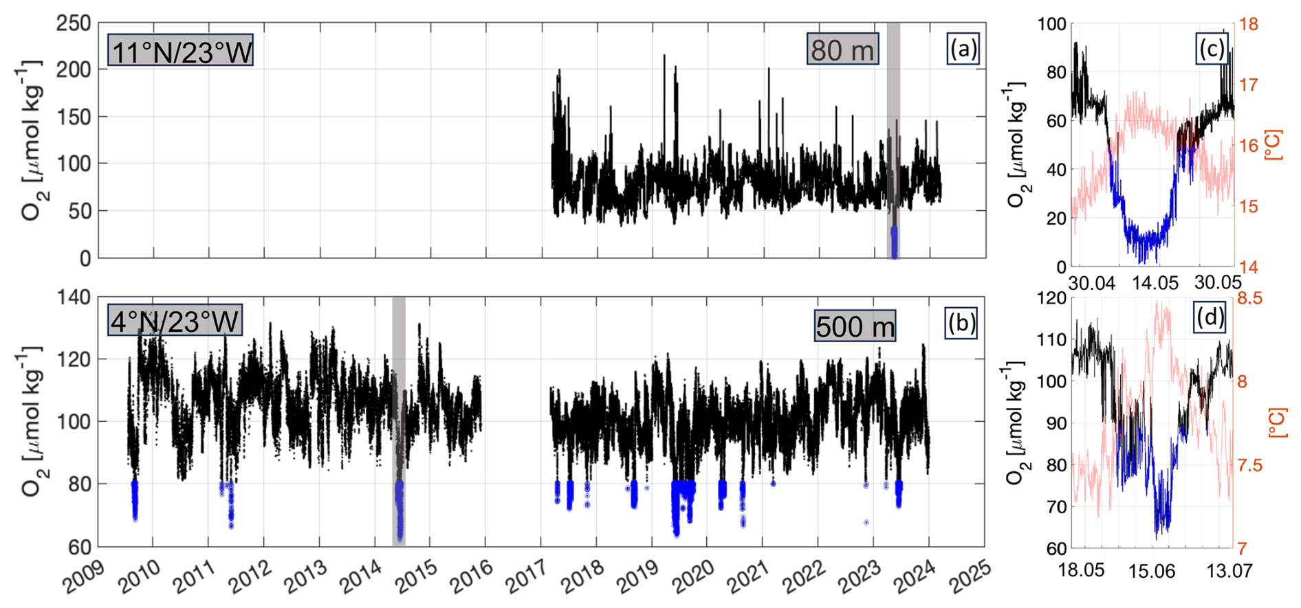
Figure 3 Time series of observed DO at (a) 80 m depth at 23° W, 11° N and 500 m depth at 23° W, 4° N shown in black. The blue color represent the lowest 10th percentile of the time series data. The grey boxes mark the timespan (date on the x axis) which is shown in (c) and (d), where the temperature is overlaid in red.

As expected, both the DO variability and amplitude of DO anomalies are generally greater at shallower depths (e.g., 80 m), due to more intense near-surface dynamics and elevated background DO concentrations. Therefore the largest DO drops were typically observed at 80–100 m. In terms of spatial variability, we see that the DO variability within the core of the deep oxygen minimum zone (OMZ) at 11° N is generally lower than at 4° N.

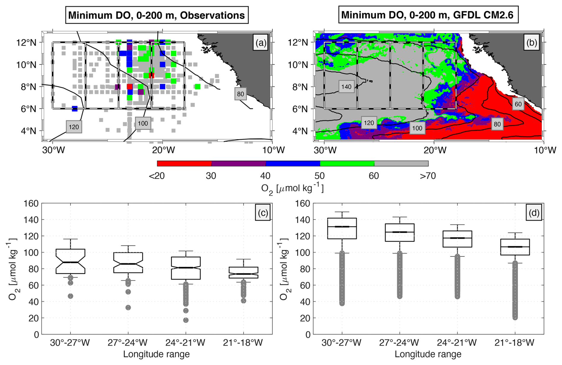
Figure 4 (a) Spatial distribution of DO profiles acquired from shipboard CTD-O observations in the tropical North Atlantic. Colored/gray dots denote DO profiles with a minimum DO concentration of lower/higher than 60 µmol kg⁻¹ in the depth range 0–200 m (red: <30 µmol kg⁻¹, violet: 30–40 µmol kg⁻¹, blue: <40–50 µmol kg⁻¹, green: <50–60 µmol kg⁻¹. (b) Horizontal distribution of DO minimum obtained in the depth range 0–200 m and from the last 20 years of GFDL CM2.6 model run. Black contour lines in (a) and (b) show 0–200 m minimum of mean DO distribution (similar to filled contours in Fig. 2a and b). Dashed boxes denote different regions of interest for boxplots shown in (c) and (d). (c) Boxplots for 0–200 m minimum of DO profiles, that are shown for four different regions by the dashed boxes in (a). Thick line in each boxplot denotes median and notches show 95 % confidence interval. Upper and lower whiskers denote 10 % and 90 % quantiles. Grey dots below the lower whiskers show 10 % lowest DO events. (d) Similar to (c), but boxplots shown for 0–200 m minimum of DO profiles that were taken from the last 20 years of GFDL CM2.6 model run.

In addition to the moored DO observations, there are multiple years of shipboard measurements in the region. From all these shipboard observations, low-DO extremes are identified by searching for the minimum DO concentration in the upper 200 m of every single CTD-O profile. A low-DO extreme event was defined when DO was below a threshold of 60 µmol kg⁻¹, which represents the 10-percentile of all DO observations (74 of 976) in the area 6–12° N, 30–18° W (Fig. 4a and c). This threshold is more than 20 µmol kg⁻¹ below the climatological DO concentration in the ETNA (Fig. 2a and b). Considering the absolute DO concentration allowed us to derive a distribution of low-oxygen extremes, which is not masked by the mean distribution. Lowest DO concentrations below 40 µmol kg⁻¹ (7 of 976 CTD-O profiles) in the near equatorial region (south of 12° N) remarkably occurred not east of 21° W, where profiles are located within a distance of 8° to the African coast, but in the “open-ocean” region west of it (24–21° W (Fig. 4a). Further to the west (>24° W), lowest DO concentrations were found again just above 40 µmol kg⁻¹. This is in contrast to the more coastal upwelling region north of 12° N, where very low-DO extremes can also be observed near the coast (see Fig. 1 or Schütte et al., 2016b). In order to scale for the different number of CTD-O profiles in the four regions shown in Fig. 4a (5 %, 9 %, 61 % and 25 % of the profiles for the boxes 30–27° W, 27–24° W, 24–21° W, 21–18° W), we estimated the relative distribution and calculated the 10-percentile threshold in every box (Fig. 4c). This threshold is lowest in the open ocean (24–21° W), whereas the mean DO distribution is increasing from the eastern boundary towards west. This counterintuitive distribution of low-oxygen extremes, which is against the mean DO gradient, suggests that DO depleted water generally cannot be purely advected from a remote region at the eastern boundary, that is poor in DO. Locally enhanced biological activity associated with enhanced DO consumption must play a role as well.

The two events with the lowest dissolved oxygen (DO) concentrations were measured as 17  µmol kg⁻¹ by a CTD at 60 m depth at 8 µmol kg⁻¹ were recorded by a mooring at 80 m depth at 11° N/23° W. These two low-oxygen extremes were well below the climatological average minimum DO concentration for the whole ETNA (40 µmol kg⁻¹ in the deep OMZ, Brandt et al., 2015). We shall note, that no CTD-O profiles were available in this data set for the eastern boundary region within about 2° longitude off the African coast.

4.2 Association of low-oxygen events with subsurface high-baroclinic mode vorticies

For the majority of the ship based data and for the mooring at 11° N/21° W additional observations of hydrography, zonal and meridional velocity are available indicating the passage of anticyclonically and cyclonically rotating vortices associated to the low-oxygen events. At the mooring position the low-oxygen events #01, #02, #03, #04 and #07 were most likely related to the passage of subsurface intensified vortices, whereof events #02, #04 and #07 were associated with anticyclonic vortices and events #01 and #03 with cyclonic vortices (Fig. 5). Note, that we explicitly refer here to the notation vortex, since we could not derive the vortices' radii in order to differentiate between mesoscale and submesoscale. For the anticyclonic vortices, meridional velocity was observed with maximum northward and southward flow taking place at the beginning and the end of each low-DO period. Zero crossing was observed in between at around the time, when DO was at its minimum (Fig. 5e–h). Corresponding time series of potential density derived from hydrographic observations, conducted next to the DO sensors, indicated a depression of isopycnal surfaces in the depth range below 100 m. Time series of velocity and potential density agree well with the dynamical understanding and passage of westward propagating eddies (van Leeuwen, 2007) through the mooring site. Zonal velocity was either small or showed maximum flow during time periods of minimum DO, depending whether the eddy has crossed the mooring site either with its core or with one of its meridional flanks. Zonal velocity vanished at the beginning and the end of each of the three events.

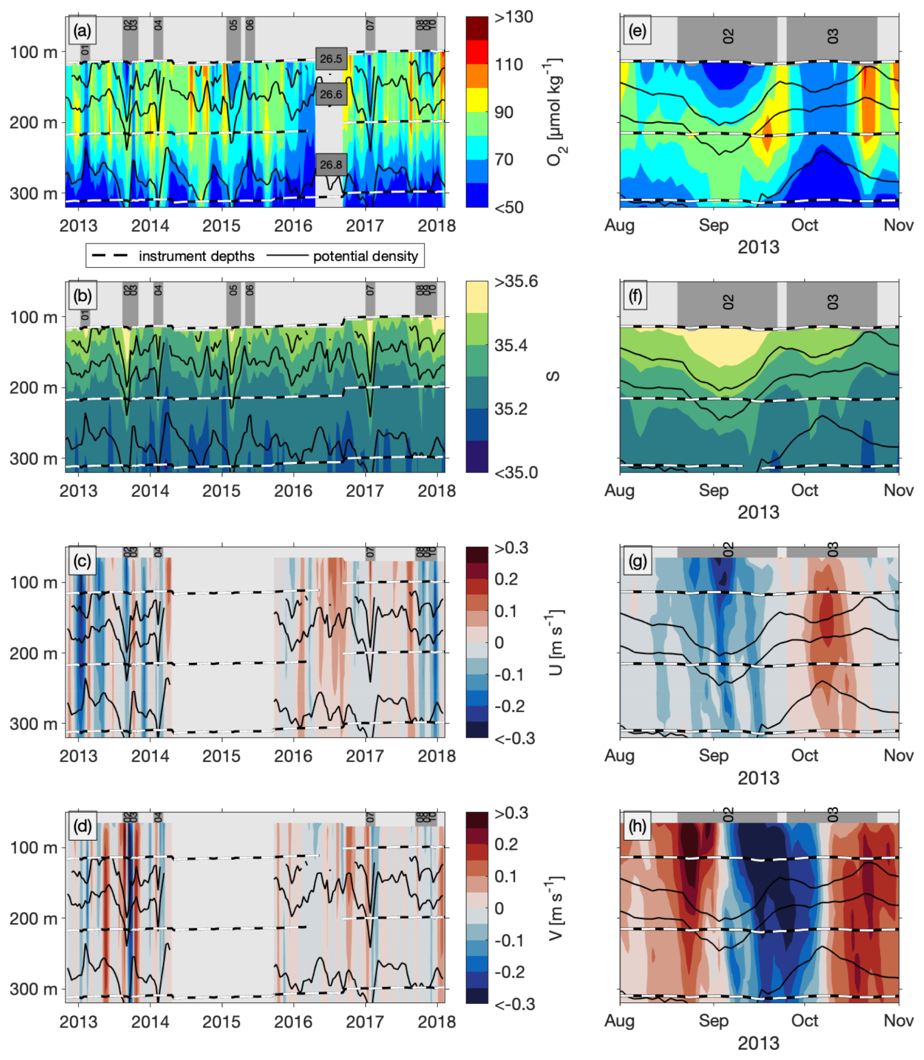
Figure 5 Time series of observed (a) DO, (b) salinity, (c) eastward and (d) northward velocity from moored observations at 11° N/21° W in the upper 300 m as a 10 d average (color shading). Black lines denote depth of potential density surfaces 26.5, 26.6 and 26.8 kg m⁻³. Black-white dashed lines denote depths of DO sensors – in (a), (c) and (d) – and salinity sensors (in b). Gray bars with numbers 01–10 in the top of these panels denote time periods of low-DO events (#01 to #10). Note, that no velocity observations are available for low-DO events #05 and #06. Panels (e)–(h) show corresponding 2 d averaged time series for the 90 d time period around low-DO events #02 and #03.

During events #01 and #03, that are associated with the passage of subsurface intensified cyclonic vortices, we found a depression of isopycnal surfaces above 150 m and a heave of isopycnal surfaces below (cf. McGillicuddy, 2015, denoted as eddies of type Thinny). This is associated with a maximum in stratification at about 150 m depth. The time series of zonal and meridional velocity, respectively, showed maximum values at a similar depth with a transition from westward to eastward (event #01) and southward to northward (event #03) velocities during the time of maximum stratification. In contrast to the anticyclonic vortex events (#02, #04 and #07), the DO minima during the passage of the two cyclonic vortex events (#01 and #03) were of similar intensity at 100 and 200 m depth, with no separation from the deep OMZ at 300 m by an intermediate DO maximum. Though, during both events the minimum DO at 100 m was well below the average DO concentration that was observed for time periods without any vortex event. We shall explicitly note, that the characteristics for zonal and meridional velocity during event #01 were swapped compared to the other eddy events (#02, #03, #04 and #07). We can only speculate whether this cyclonic vortex has crossed the mooring site in a more meridionally directed pathway.

The vertical structure of these vortices could not be identified for the near surface layer and the deep ocean, since moored hydrographic and velocity observations were only available between 100 m (60 m for velocity) and 800 m depth. This made it challenging to distinguish among surface intensified and subsurface intensified (but at shallow depth) vortices. The most likely subsurface intensified vortex was associated with event #02, showing extreme velocity (both zonal and meridional) slightly below the shallowest depth of available observation accompanied by an oxygen minimum of 39 µmol kg⁻¹. Notably, none of these vortices exhibited a clear surface signature in satellite data that could be unambiguously associated with the subsurface features

4.3 Horizontal extent of the low-oxygen high-baroclinic mode vorticies

The ship-based data, which cover the region spatially, are significantly better suited than the stationary moored data for assessing the spatial extent of the HBVs. Repeated meridional ship sections between 6–12° N along 23° W, available over a distance of at least 300 km, captured 15 events with DO concentrations well below 60 µmol kg⁻¹ in the upper 200 m (Table 1, Fig. 6). All DO minima were found directly below the shallow oxycline at depths between 45 and 90 m (corresponding to surfaces of potential density between σ_θ=26.2 and 26.4 kg m⁻³). The meridional resolution of CTD-O measurements did not allow for a proper identification of the meridional core position of the low-DO extremes, but their extent was found with roughly 1° in latitude in maximum. The low-DO cores vertically extended to the isopycnal σ_θ=26.5 kg m⁻³ (150 m depth) and were separated from the deep OMZ by an intermediate DO maximum located at about σ_θ=26.7 kg m⁻³ (between 200 and 300 m), which rules out a simple vertical displacement of the vertical gradient.

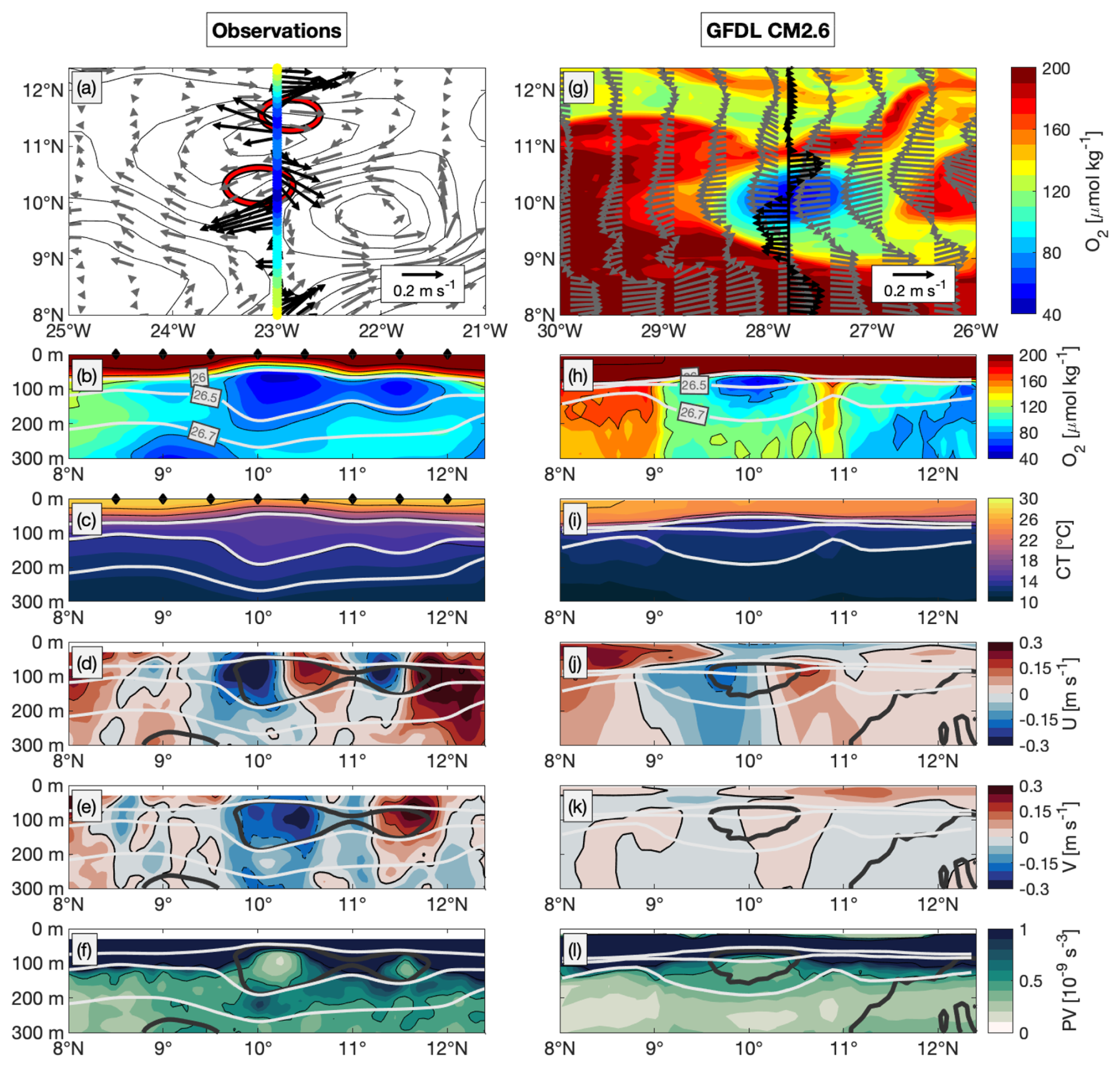
Figure 6 (a) Current velocity (black arrows) and DO (colored dots) at 80 m depth along 23° W and between 8 and 12° N obtained from along-track shipboard ADCP observations and CTD-O observations between 23 and 25 July 2009 (cruise Ron Brown 2009, see Table 1). Grey arrows show geostrophic velocities and black contours show sea level anomalies from satellite altimetry data on 24 July 2009. Red circles denote positions and extent of the two eddies, identified and reconstructed from shipboard ADCP observations at 80 m. Latitude-depth sections of (b) DO, (c) conservative temperature, (d) zonal velocity, (e) meridional velocity and (f) PV between 8 and 12° N obtained from CTD-O observations along 23° W (same period to a). Black diamonds at the top of panels (b) and (c) denote actual latitudes of CTD-O profiles. Thin gray lines in panels (b)–(f) denote surfaces of potential density. In panels (d) and (e), solid black and dashed black lines denote 0.15 m s⁻¹ velocity intervals. Thick dark gray lines in panels (d)–(f) denote DO contours of 70 µmol kg⁻¹. (g)–(l) are analog to (a)–(f), but taken from GFDL CM2.6 model simulation for model date 23 Mar 0197. Gray arrows in (g) denote surface velocity. Black arrows denote current velocity and colored contours show DO distribution both at 77 m depth along ∼28° W. (h)–(l) show respective latitude-depth sections along ∼28° W for the same model date. Thick dark gray lines in panels (j)–(l) denote DO contours of 90 µmol kg⁻¹.

Table 1 Low-DO events (below 60 µmol kg⁻¹) found in the upper 200 m during meridional CTD-O ship sections along 23° W between 7 and 12° N. Only those low-DO events are listed, where meridional sections of DO, hydrography and velocity were available (spanning a latitude range of minimum 3°). Columns from left to right denote DO minimum between 0 and 200 m, corresponding depth, latitude and research cruise with date of the CTD-O profile. The last three columns denote type, core position and radius of related eddy, that was analyzed with the eddy identification method. ACE events are marked in bold (the abbreviation ACME stands for anticyclonic mode water eddy). As an example, the event in the third row (Meteor 119/1, 17 September 2015) is presented in Fig. 4.

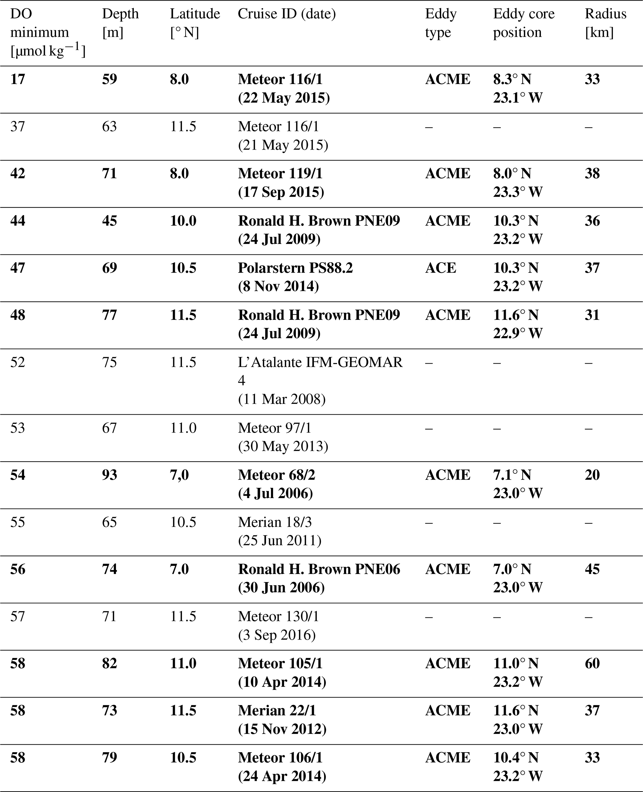
We analyzed the distribution of zonal and meridional velocity at the depth of the DO minimum using an eddy identification algorithm as described in Sect. 3.3.1. Strikingly, 66 % (10 of 15) of the low-DO events could be related to HBVs, where radii were identified between 20 and 45 km (average 34 km) (Table 1, Fig. 6b and d). The radii are substantially smaller than the typical mesoscale (first baroclinic Rossby radius of deformation) at these latitudes being at the order of 100 km or more. Instead, these eddies have a confined baroclinic structure, which is associated to higher baroclinic modes and corresponding smaller Rossby radii of deformation as is shown in detail in Sect. 4.4. The HBVs' horizontal core positions are estimated from the current velocities and closely match the meridional position of the low-oxygen extremes (cf. 3rd and 6th column for bold marked events in Table 1; Fig. 6a and b). Note, that the derived HBVs' zonal core position range between 23.3 and 22.9° W, whereas for the low-oxygen extremes, only the meridional position along the 23° W section can be identified. Notable is the simultaneous occurrence of two HBVs observed during one cruise in 2009 at positions 10.3° N/23.2° W and 11.6° N/22.9° W (Fig. 6a–f). These two HBVs were meridionally cut through their eastern and western flank, respectively, and were both observed with DO concentrations well below 50 µmol kg⁻¹ (Fig. 6a and b).

Both HBVs were identified to be anticyclonic and subsurface intensified, as shown by the anomalously weak stratification along 23° W at subsurface depth, which is indicated by the thickening of isothermal and isopycnal layers at the depth range of the DO minimum core (Fig. 6c). The vertical extent of the HBVs (characterized by displaced isopycnal surfaces or zonal velocity) reached at least down to about 250 m and covered the vertical extent of the low-DO cores. The estimated radii are 36 and 31 km and thus considerably smaller than the first baroclinic Rossby radius of around 90 km at these latitudes. For none of the 10 anticyclonic HBVs, we could identify any anticyclonic signature from satellite altimetry observations (Fig. 6a). One reason might be that the resolution of gridded SLA from conventional altimetry (in time and space) is not sufficient to resolve such small-scale features. Another reason could be the fact that the eddies are strongly confined to the thermocline (below 30–50 m) and often do not have a surface signature.

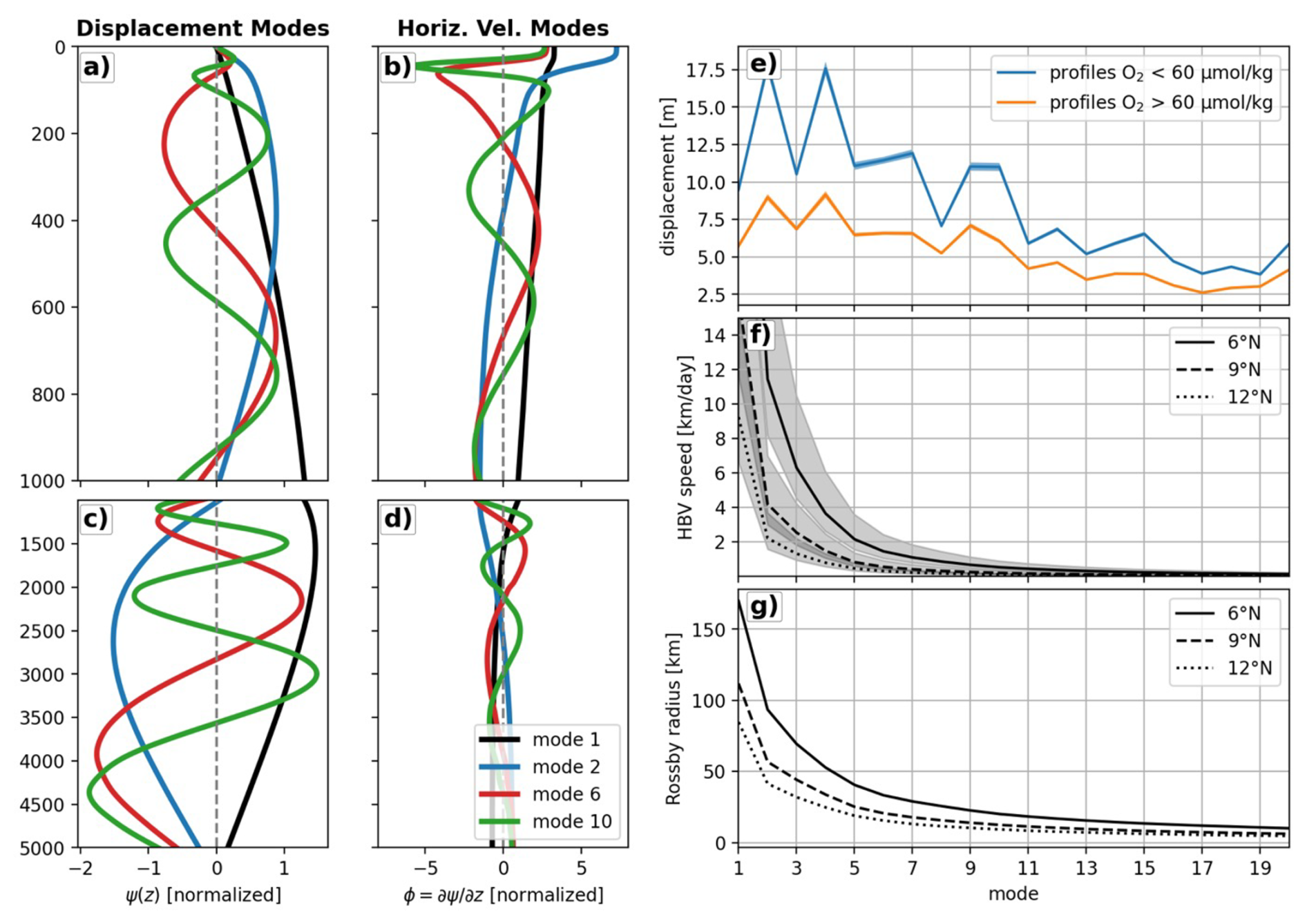
Figure 7 Dimensionless vertical structure functions of baroclinic modes 1, 2, 6 and 10 for (a, b) isopycnal displacement, Ψ_n, and (c, d) horizontal velocity, ϕ_n, obtained from the hydrographic profile of the World Ocean Atlas at 9° N/23° W. (a) and (c) (b and d) show depth range 0 to 1000 m (1000 m to bottom). (e) Mean amplitudes of first 20 vertical displacement modes calculated through modal projection of hydrographic profiles from 23° W ship sections. Blue solid line denotes mean amplitude distribution, that is related to all hydrographic profiles with a minimum DO smaller than 60 µmol kg⁻¹ in the upper 200 m (i.e. low-DO events that are summarized in Table 1). Orange solid line denotes mean amplitude distribution for all other hydrographic profiles along 23° W. Respective shadings denote standard error of the mean amplitude over all 1000 realizations. (f) Theoretical translation speed of high-baroclinic Rossby waves (HBVs) for the first 20 vertical modes between 6 and 12° N along 23° W (see Eq. 9). The solid, dashed and dotted black lines represent Ro=0.5, while the shaded area indicates the range $\mathrm{0.3}<Ro<\mathrm{0.7}$. (g) Rossby radii of deformation for the first 20 vertical modes. In both (f) and (g), solid, dashed, and dotted lines correspond to values at 6, 9, and 12° N along 23° W, respectively.

4.4 Vertical structure of low-oxygen high-baroclinic mode vorticies

The decomposition of a disturbed density profile into vertical baroclinic modes gives evidence about both the theoretical radius (Rossby radius) and propagation speed for this disturbed state (see Sect. 3.1). Here, we did a vertical baroclinic mode analysis for the meridional section along 23° W between 6 and 12° N, which allowed us a direct comparison against the spatially resolved low-DO HBVs observed during the respective ship sections. The vertical structure of the first 20 baroclinic modes was obtained from the climatological hydrographic distribution (Fig. 7a–d). For all individual CTD-O profiles, we derived displacement profiles, ξ, and calculated vertical mode amplitudes x_n via modal decomposition (as described in Sect. 3.1). We then clustered all x_n (i) related to a low-DO event (Table 1) and (ii) not related to a low-DO event (i.e. all other profiles along 23° W between 6 and 12° N), and calculated an average amplitude distribution (Fig. 7e). For low-DO events, we found substantially enhanced amplitudes at all modes, but particularly at mode 2, 4, 7, 9 and 10 compared to the average amplitude distribution that is related to no low-DO events (Fig. 7e). These higher baroclinic modes n>4 (exemplarily shown for mode 6 and 10 for 9° N/23° W in Fig. 7a and c for vertical displacement and pressure/horizontal velocity, respectively) have zero crossings in the upper few hundred meters, that are of similar vertical length scale compared to the vertical extent of low-DO HBVs (near-surface to 250 m, see Sect. 4.2.1). The lower baroclinic modes (e.g. mode 2) have a much larger vertical length scale and are not capable of describing the vertical structure that is related to low-DO HBVs. The corresponding Rossby radius of deformation for vertical baroclinic modes 4 to 10 was found from $R_{\mathrm{d},\mathrm{4}}=\mathrm{47}$ km to $R_{\mathrm{d},\mathrm{10}}=\mathrm{18}$ km at 6° N/23° W and from $R_{\mathrm{d},\mathrm{4}}=\mathrm{24}$ km to $R_{\mathrm{d},\mathrm{10}}=\mathrm{9}$ km at 12° N/23° W (Fig. 7g). These radii are well below the first baroclinic Rossby radius of deformation ($R_{\mathrm{d},\mathrm{1}}=\mathrm{152}$ km at 6° N/23° W and $R_{\mathrm{d},\mathrm{1}}=\mathrm{80}$ km at 12° N/23° W) and are close to the average radius of 34 km that was identified for the observed low-DO eddies (cf. Table 1 and Sect. 4.3).

4.5 Source waters of high-baroclonic mode vorticies

The determination of the physical origin of subsurface HBVs, that are associated with the observed low-DO events, is not straight forward. A backtracking algorithm based on satellite altimetry observations as used in other studies for more poleward eddies (Chelton et al., 2011; Schütte et al., 2016a) is not applicable here, since these near-equatorial HBVs are hardly captured in the respective SLA products (Fig. 6). Instead, we derived water mass characteristics from all CTD-O profiles (Fig. 4a) located in the two boxes [24–21° W, 6–12° N] and [21–18° W, 6–12° N] for a conservative temperature range that corresponded to the depth range of the shallow DO minimum. A mean profile of absolute salinity was calculated for the two boxes and was used as a reference in order to calculate anomalies of absolute salinity as a function of potential density for every single CTD-O profile (Fig. 8). For both boxes, we clustered the salinity anomaly profiles into two classes, that were defined by the minimum DO concentration in the upper 200 m to be either below or above the threshold of 60 µmol kg⁻¹.

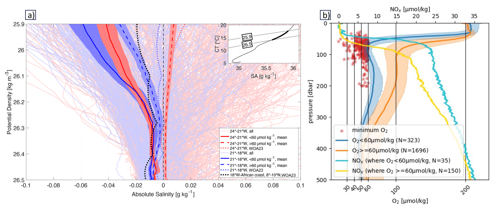
Figure 8 (a) Large panel: anomalies of absolute salinity as a function of potential density in the eastern tropical North Atlantic for two different box regimes (Red: 24–21° W, 6–12° N/Blue: 21–18° W, 6–12° N). The boxes are highlighted in Fig. 4. The anomalies are referenced to the mean profile of absolute salinity that was calculated from all hydrographic profiles found in both boxes. Thin solid lines denote all individual profiles and thick solid (dashed) lines show the average of the profiles, that are related to minimum DO concentrations below (above) 60 µmol kg⁻¹ in the upper 200 m. Shadings to the average profiles illustrate the respective standard errors (see text for details). Blue and red dotted lines denote climatological profiles for the two boxes. Black dotted line shows the climatological profile for a third box (18° W-African coast, 8–10° N), which defines the near-coastal regime off West-Africa. Inlet panel: mean characteristics of absolute salinity versus conservative temperature for the box 24–18° W, 6–12° N, taken from all CTD-O observations in this regime. Thick black line denotes the characteristics in the potential density range 25.9 to 26.5 kg m⁻³ and is the reference profile for the anomalies shown in the large panel. (b) The blue curve shows the median of all oxygen CTD profiles with a minimum below 60 µmol kg⁻¹ in the upper 200 m. The red stars indicate the depths and dissolved oxygen concentration of these minima. Orange curves represent profiles with a minimum above 60 µmol kg⁻¹. Shaded areas indicate the standard deviation. The turquoise line depicts the mean nitrate profile for the profiles with oxygen minima below 60 µmol kg⁻¹, and the yellow line shows the mean nitrate profile for the profiles with minima above 60 µmol kg⁻¹.

Along-isopycnal gradients of mean salinity are weak (i.e. small spiciness) in the considered region [24° W – African coast, 6–12° N], as shown by the water mass characteristics obtained from the climatological distribution World Ocean Atlas 2023 for the two boxes as well as for the near-costal area east of them (Reagan, 2023; Garcia, 2024). The westward salinity increase along isopycnal surfaces is roughly 0.01 to 0.02 g kg⁻¹ per 5° (from the African coast at 17° W to about 22° W) in the potential density range between 26.1 and 26.4 kg m⁻³. This weak isopycnal gradient does not allow for a differentiation of water mass characteristics from individual CTD-O profiles.

However, water mass characteristics for low-DO and high-DO profiles were found to be significantly different from each other, when isopycnally averaging over all respective profiles. For the western box [24–21° W, 6–12° N], low-DO profiles were on average lower in salinity (compared to high-DO profiles) and they were found to be close to the average salinity anomaly profile from the eastern box [21–18° W, 6–12° N], suggesting that water masses related to low-DO profiles have their origin closer to the eastern boundary. However, the tropical low-DO extremes appear in the open ocean far away from the eastern boundary. The westward intensification of these events (Sect. 4.1, Fig. 4), that are often related to HBVs (Sect. 4.2), suggests an unexpected long isolation of the DO depleted water masses in the otherwise oxygen rich open ocean.

To further support the persistence and longevity of HBVs, we analyzed CTD observations of oxygen and nitrate inside and outside of low-oxygen events. Figure 8b shows the median oxygen profiles for CTD casts with a minimum in the upper 200 m of the water column below 60 µmol kg⁻¹ (blue curve) and those above 60 µmol kg⁻¹ (orange curves). Mixed layer oxygen concentrations for both cases indicate increased near-surface biological productivity of HBVs compared to outside of HBVs. The red stars indicate the depths and dissolved oxygen concentrations of the observed oxygen minima, clustering between 80 to 120 m depth. Corresponding nitrate profiles are shown in turquoise (<60 µmol kg⁻¹ oxygen) and yellow (>60 µmol kg⁻¹ oxygen). The results reveal substantially lower oxygen concentrations between 80–250 m inside HBVs, accompanied by elevated nitrate levels, consistent with enhanced accumulated ongoing biologically remineralization due to enhanced productivity and/or “older” water. This observational evidence indicates that HBVs consist of persistent, isolated water masses rather than short-lived anomalies.

4.6 Origin and temporal evolution of high-baroclinic mode vorticies based on model simulations

Outputs from the GFDL CM2.6 ocean model is used to investigate the origin and temporal evolution of these unusual vorticies. We used the last 20 years of simulations for a regime similar to that considered in the shipboard observations. From Fig. 2, we already know that the model captures the main features of the mean state of the oxygen distribution. To assess whether low-oxygen events occur with similar frequency in the model and whether they are likewise associated with HBVs, we conducted analyses analogous to those performed on the observations (Sect. 4.1, Fig. 4; and Sect. 4.3, Fig. 6) using the model data.

First the horizontal DO distribution was calculated by taking the temporal and vertical (0–200 m) minimum of the simulated DO similar to the observations (Fig. 4b). In the latitude range 6–12° N, lowest DO below 30 µmol kg⁻¹ is found close to the African coast (east of 18° W). In general, the basin wide gradient of minimum DO is positive towards west, being in agreement with the zonal gradient of the mean simulated DO distribution (Fig. 2b). Strikingly, minimum DO is lower in the region 30–24° W, 8–12° N than in the region east of it (24–21° W). The threshold for the DO 10-percentile (100 µmol kg⁻¹) does not change over this longitude range, whereas the mean DO distribution is increasing towards west (lower whiskers versus box centers in Fig. 4d). The open ocean minimum of the DO distribution that is found in the region 30–24° W, 8–12° N is in good qualitative agreement (though located further west) with the observed DO distribution (Fig. 4b versus Fig. 4a). In the longitude range 24–21° W, low-oxygen events are less likely. It should be noted that Fig. 4a and b compare individual shipboard observations with the 20-year model climatology. Observations represent snapshots of specific events, whereas the model averages over a longer temporal period. Consequently, apparent differences in the zonal distribution of low-DO extremes are expected and do not necessarily indicate a systematic model bias.

From the GFDL CM2.6 model, we identified a HBV with a low-DO core in the near-equatorial open ocean as exemplarily shown at the position 10° N/28° W (Fig. 6g–l). The spatial extent is comparable to our observational results (Fig. 6a–f). A meridional cross section through the simulated HBV reveals the low-DO core at 80 m depth (isopycnal surface 26.5 kg m⁻³) with a lateral extent of about 1° in latitude and a vertical extent between about 50 and 150 m (Fig. 6h). The minimum DO is lower than 60 µmol kg⁻¹, whereas DO outside the HBV is at values above 150 µmol kg⁻¹. Distributions of conservative temperature and potential density show shallowing and deepening isopycnal surfaces above and below the DO minimum, respectively, indicating a weakened stratification and consequently low PV at the low-DO core (Fig. 6i). The HBV's velocity signature is strongly confined to subsurface depths and vanishes above 50 m (Fig. 6j and k). In particular, surface velocity does not show any coherence with the subsurface velocity field at depth of the HBV (Fig. 6g). This substantiates our observational results that these HBVs can hardly be identified from the surface geostrophic velocity field obtained from satellite observations. The HBV core exhibits low PV water, where minimum PV is found slightly deeper than the DO minimum (Fig. 6l). This low PV water core is laterally isolated from the surrounding high PV water, but also separated from the deeper low PV water through an intermediate PV maximum along the isopycnal surface 26.7 kg m⁻³. This isolation is the prerequisite for a persistent eddy with a long-life time. The model tends to slightly underestimate PV and associated O₂ anomalies, indicating somewhat weaker eddy coherence compared to observations. At the same time, due to reduced dissipation in the circulation model, we expect lifespans of the eddies to be slightly prolonged. Additionally, the MiniBLING model does not fully account for remineralization processes in the mesopelagic zone, which likely leads to an underestimation of oxygen consumption. Taken together, this implies that HBVs in the model appear with weaker anomalies but with an artificialy prolonged liefespan.

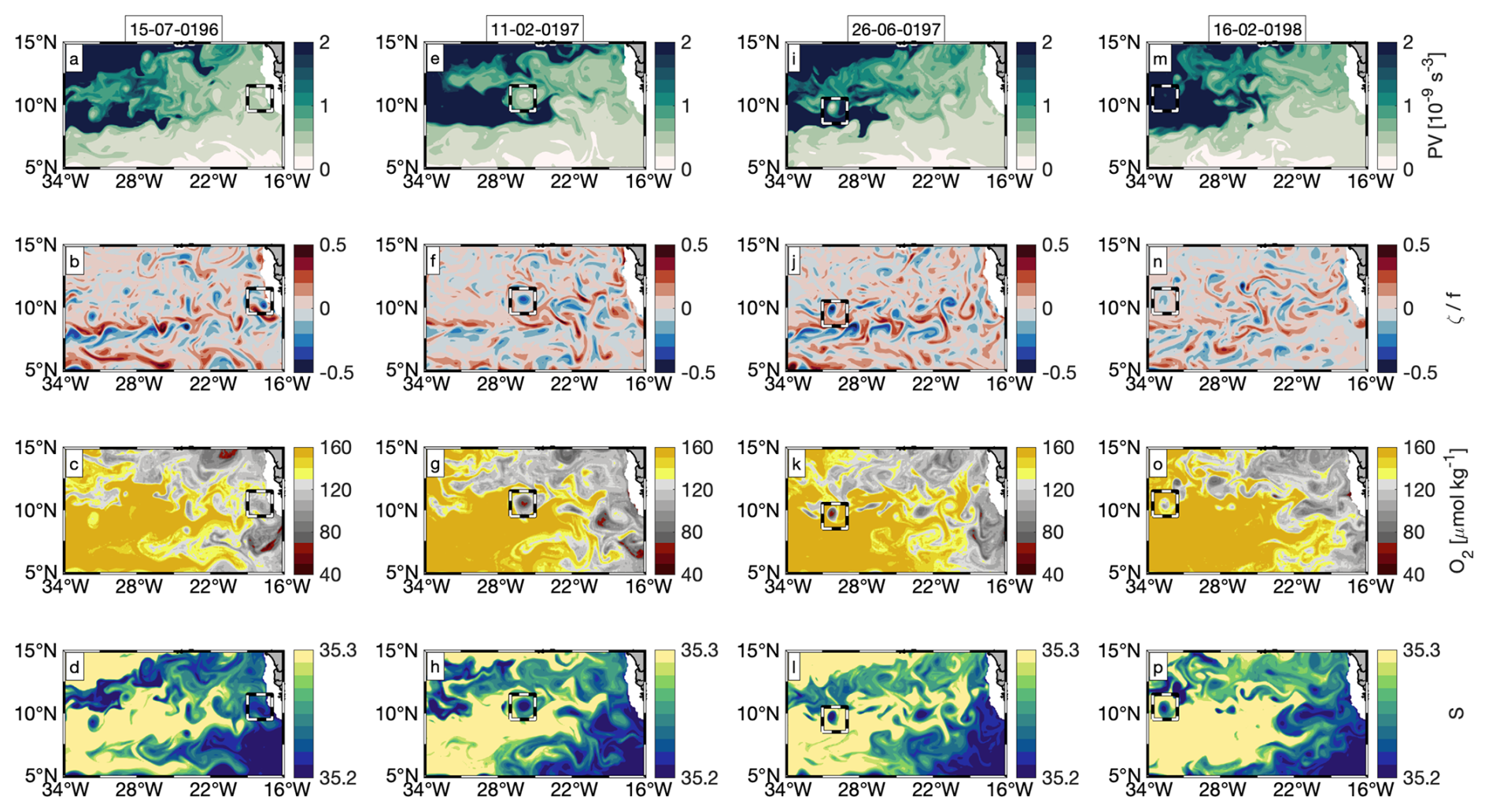
Figure 9 Model snapshots of PV on isopycnal surface 26.6 kg m⁻³ (a, e, i, m), relative vorticity over f, DO and salinity on isopycnal surface 26.5 kg m⁻³ (b, c, d, f, g, h, j, k, l, n, o, p) for different phases (different columns) of an anticyclonic HBV (respective time indicated above each column with T=0/211/346/580 d: formation/strongest peculiarity/weakening/ decay. Black-white dashed box in each sub panel denotes HBV position.

In the following, we present the temporal evolution of the HBV from the time of formation to the decay. Figure 9 shows model snapshots with horizontal maps of PV, relative vorticity normalized by f (so that its magnitude is equal to Rossby number), DO and salinity for four different time points throughout the HBV's lifetime. Figure 10 shows time series of different physical and biogeochemical variables for the HBV core position.

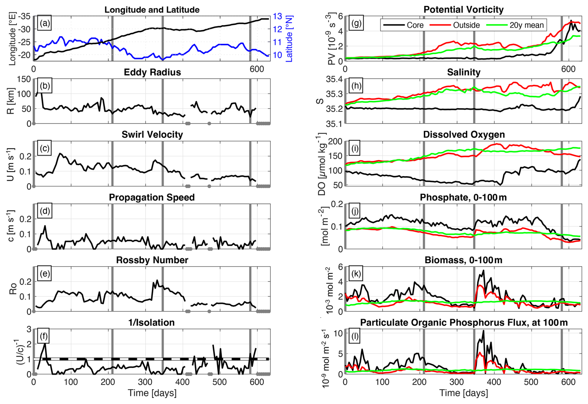
Figure 10 Time series of different variables related to the core of the modelled subsurface intensified eddy shown in Figs. 6g–l and 9. Time is given as elapsed days since eddy detachment from the African coast. Vertical gray lines in each panel denote time points for horizontal maps shown in Fig. 9 (0, 211, 346 and 581 d). (a) Longitude (black line) and latitude (blue line), (b) Eddy radius, (c) Eddy swirl velocity, (d) Eddy propagation speed, (e) Rossby number, (f) Inverse of isolation parameter (black line). Black-white dashed line denotes threshold, below which the water is trapped in the eddy core (swirl velocity > propagation speed). (g) Potential vorticity, (h) salinity, (i) DO, (j) phosphate, (k) biomass, (l) flux of particulate organic phosphorus. Variables are given for the following layers. In panels (a)–(f) and (h)–(i): isopycnal surface 26.5 kg m⁻³. In panel (g): isopycnal surface 26.6 kg m⁻³. In panels (j) and (k): integral over 0–100 m. (l) at 100 m. For the right column (panels g–l), black lines show value in eddy core, red lines show mean values outside the eddy (average between 1 and 3° of longitude/latitude around the eddy core position) and green lines show 20-year model mean that is given at the respective position of the eddy core. In panels (b)–(f), gray dots at zero line denote time points, where no estimate was possible.

The HBV has its origin at the eastern boundary at 10° N/18° W, where low PV water (Fig. 9a) with anticyclonic vorticity (Fig. 9b) is deflected offshore and provides the precondition for the eddy formation. The offshore deflected water carries typical water mass characteristics from the eastern boundary: low DO and low salinity (Fig. 9c and d). During westward propagation into the open ocean, the HBV enters high PV waters. 211 d after formation, it reaches 10.5° N/26° W with low PV (Fig. 9e) and high negative relative vorticity (Fig. 9f) in its core. The coherent eddy is strongly isolated from surrounding high PV water as shown by the intensified DO minimum (Fig. 9g) and low salinity (Fig. 9h) in its core. In the following 5 months the HBV propagates further westward, but is disturbed by high PV water, that is advected from the western tropical Atlantic. This leads to a weakening of the HBV with a smaller low PV core (Fig. 9i), but still carrying pronounced negative relative vorticity (Fig. 9j), low DO (Fig. 9k) and low salinity (Fig. 9l) compared to surrounding water. The HBV eventually loses its energy and decays about 580 d after formation at 10° N/33° W (Fig. 9m and n), where the core water still appears with anomalous low DO and salinity (Fig. 9o and p).

The quick offshore deflection of coastal water, that is associated with the HBV's formation, is illustrated by the strong change in longitude (Fig. 10a) and by the high propagation speed (Fig. 10d) during the first 50 d. This deflection is more like a pulse rather than an offshore transport of enclosed water ($(U/c{)}^{-\mathrm{1}}>\mathrm{1}$, Fig. 10f), where the HBV stabilizes after that time at a radius of 50 km (Fig. 10b).

From day 80 to day 300, the HBV continuously propagates westward until 30° W with only slight changes in latitude (10–11° N), at a propagation speed of 0.7 m s⁻¹, a swirl velocity between 0.1 and 0.2 m s⁻¹ and a radius of 50 km (Rossby number between 0.1 and 0.2) (Fig. 10a–f). The strong isolation ($(U/c{)}^{-\mathrm{1}}<\mathrm{1}$) over that time keeps the core water constantly low in PV and salinity, while surrounding waters increase in PV and salinity during eddy westward propagation (Fig. 10g and h). DO continuously decreases from roughly 95 to 50 µmol kg⁻¹ over several months, corresponding to an average DO consumption rate of about 0.16 µmol kg⁻¹ d⁻¹ (Fig. 10i). This apparent decline should be regarded as a lower limit, as ventilation and mixing processes would partly offset oxygen loss. In the upper part of the eddy, enhanced nutrient concentration is associated with increased biomass production, which leads to enhanced export of organic matter between days 100 and 300 (Fig. 10j–l). The associated increased respiration and the strong isolation both lead to the development of this substantial DO deficient zone. Note, that the magnitude and timescale of this decrease are broadly consistent with observed low-oxygen events in the region, though specific rates from the model should be interpreted cautiously.

The high PV water, that is advected from the west, acts as a barrier for the HBV and westward propagation stops after day 300 (Fig. 10a and d). The HBV is deformed by the high PV water, which likely leads to enhanced isopycnal and diapycnal mixing at the eddy periphery. In fact, the HBV shrinks between days 300 and 400 as illustrated by the continuously decreasing radius from 50 to 30 km (Fig. 10b). Though, the core still shows source water characteristics with unaltered low PV and low salinity, and still holds the DO deficient zone. After day 400, the HBV starts to interact with surrounding water – partly being low in PV as well – which weakens the isolation of the HBV core ($(U/c{)}^{-\mathrm{1}}\approx \mathrm{1}$, Fig. 10f) and leads to continuous increase of PV and DO. PV strongly increases after day 550 and reaches the PV threshold of surrounding water at about day 600, where the core starts to dissolve as illustrated by the strong increase of salinity and DO after day 600.

5 Discussion

Moored time series of dissolved oxygen (DO) in the near-equatorial Atlantic (4° N up to 12° N) occasionally reveal pronounced drops in oxygen concentrations that fall significantly beneath the climatological mean. These events occur well below the mixed layer and can persist for several weeks. In addition, we found that about 8 % of all observed CTD-O profiles in the near-equatorial ETNA (25–15° W, 6–12° N) appear with anomalous low-DO (<60 µmol kg⁻¹) in the upper 200 m, which is as well below the climatological DO concentration. Until now, the causes of these extreme low-DO events have remained unclear. Mesoscale eddies with low oxygen cores – known to occur farther north around 20° N – are not expected to drive such extensive oxygen-deficient zones in the near-equatorial region, as they are not believed to persist here as coherent vortices with lifespans of several months or longer (Chaigneau et al., 2009; Keppler et al., 2018). However, the majority of these low-DO events (60 %) are clearly associated with high-baroclinic subsurface-intensified eddies (Table 1, Figs. 4 and 5). For the remaining 40 %, the velocity and density distributions did not reveal clear eddy signatures, nor did satellite data – consistent with all identified vortices, which generally lack a distinct surface signature. However, a connection to subsurface-intensified eddies cannot be ruled out a priori for these cases.

This underlines that in understanding the Earth system, a better understanding of small-scale ocean dynamics (smaller than the first baroclinic Rossby radius of deformation) is essential, as they play a crucial role in the distribution of energy and tracers as well as the regulation of biogeochemical processes. In particular, below the surface layer – where satellite observations are ineffective – our understanding of the frequency, magnitude, and impact of these small-scale ocean dynamics remains limited.

In the vicinity of the equator (<5° N/S), mesoscale dynamics dominantly appear as horizontally anisotropic waves (e.g. tropical instability waves) rather than closed circular structures. These wave-like structures, however, are not isolated enough to effectively transport or develop low-oxygen environments. The eddies with DO anomalies that we observed are relatively small and long-lived high-baroclinic vorticies (HBVs). Ship sections along 23° W exclusively revealed anticyclonic HBVs, whereas both anticyclonic and cyclonic HBVs were found from moored observations at 11° N/21° W and in the model.

5.1 Vertical and horizontal structure of the low-oxygen events and the associated high-baroclinic mode vorticies

The observed anticyclonic HBVs had a pronounced low-DO core that vertically extended from the base of the mixed layer down to several hundred meter depth (with minimum DO at depths between 45 and 90 m). The anomalous horizontal velocity of the observed anticyclonic HBVs was at maximum (maximum EKE) at the depth of the DO minimum and extended from 50 to roughly 250 m. Stratification in the observed anticyclonic HBVs' core was weak over this depth range with upward and downward displaced isopycnals above and below the depth of EKE maximum, respectively. We found an average radius of about 34 km (between 20 and 45 km) for the observed HBVs. A decomposition into vertical baroclinic modes showed, that modes 4 to 10 fit best to low-DO events that are related to these HBVs. The associated 4th to 10th baroclinic Rossby radii of deformation are between 34 and 13 km (at 9° N) and in good agreement with the observed eddy radii. The observed radii appear well below the first baroclinic Rossby radius of deformation (more than 100 km in the region) and corresponding eddies can be considered as higher baroclinic mode vorticies. Rossby numbers were below 1, with values of approximately 0.3–0.7 estimated from shipboard observations (one eddy crossing is shown in Fig. 6; others not shown) and around 0.1–0.4 in the GFDL CM2.6 model simulation (exemplarily shown in Figs. 6 or 10e).

The observed cyclonic HBVs appeared with a stratification maximum at about 150 m and a cyclonic velocity structure with maximum EKE at a similar depth. Shallow DO minima were found at 100 and 200 m throughout the transition, but without any clear separation from the deep OMZ at 300 m. This less intensified DO minimum at 100 m and the missing intermediate DO maximum at 200 m is a substantial difference to the DO distribution observed within anticyclonic HBVs. However, enhanced DO consumption has been shown to be a reasonable driver for DO depletion in a cyclonic HBV, that was observed in the western subtropical North Atlantic (Li et al., 2008). Pure upwelling or upward mixing of low-DO water from the deep OMZ cannot explain such vertically homogeneous distribution of low-DO between 100 and 300 m in cyclonic HBVs. These processes would imply either a shallowing of isopycnal surfaces or a weakened stratification within this depth range, which is contradictory to the observed deepening of isopycnals above 150 m, shallowing of isopycnals below 150 m and consequently the intensified stratification at 150 m (Fig. 5, Event #03). Due to the increased stratification, the thickness of the intermediate DO maximum layer (that is associated with isopycnal 26.6 kg m⁻³) is reduced and very likely not resolved by the sparsely distributed number of DO sensors.

We could not collocate any clear signals in SLA or SST from satellite observations with the in situ observed HBVs. Shipboard observations showed a strongly weakening velocity signature toward the surface. Also the simulated HBVs from GFDL CM2.6 model showed similar characteristics as the observed vorticies and no signature could be found from the surface velocity. Moreover, the resolution and interpolation scheme for the gridded SLA data likely do not allow to properly capture geostrophic structures at scales of smaller than about 40 km. These are likely reasons, why near-equatorial subsurface eddies are hardly identified from satellite products. If higher resolution satellite products from SWOT will allow to detect the HBVs remains to be seen, though what we see from the in-situ observed structure and the model results we conjecture that the high baroclinic mode HBVs tend to “hide” below the surface/mixed layer base.

5.2 Origin, lifetime and evolution of the oxygen content of high-baroclinic mode vorticies

Water mass characteristics derived from shipboard observations showed that open ocean water masses with DO below 60 µmol kg⁻¹ in the upper 200 m (often associated with HBVs) likely originate from the eastern boundary, where South Atlantic Central Water contributions exceed those of North Atlantic Central Water. Model results are in agreement as they show the formation of a low-DO HBVs with low PV in its core off the African coast at about 10° N/18° W. Hence, it is expected that the generation mechanism is consistent with previous studies on HBV formation, in which the interaction between the mean flow and sharp topographic curvature leads to the formation low-PV waters within the bottom boundary layer, and the shedding of HBVs (D'Asaro, 1988; Molemaker et al., 2015; Thomsen et al., 2016; Srinivasan et al., 2017; Dilmahamod et al., 2022).

The simulated HBV analyzed here propagated westward far into the open ocean over a distance of 1600 km (10° N/33° W) and lasted for 600 d (average propagation speed of 2.6 km d⁻¹). For the observed HBVs, we could not derive propagation speeds in a similar way. Instead, we followed an approach by Nof (1981) and Rubino et al. (2009), who formulated the westward translation of isolated high baroclinic eddies on a plane (Eq. 9). Considering a Rossby radius between 35 and 50 km and a Rossby number between 0.3 and 0.7 (taken as characteristic scales from the observed HBVs corresponding to the vertical baroclinic mode 4) yields a propagation speed between 1.1 and 5.4 km d⁻¹. This is in good agreement with the propagation speed obtained from the simulated HBV. Considering the origin of the observed low-DO HBVs at the eastern boundary (cf. Sect. 4.4), a propagation speed at 1.1–5.4 km d⁻¹ yields a propagation time of 100 to 500 d to propagate a distance toward 23° W (around 550 km). The fact, that these high baroclinic low-DO HBVs are not captured by satellite products, prevents both backtracking to their origin and estimating their lifetime directly.

In contrast to anticyclonic HBVs, cyclonic HBVs were only detected twice in the mooring time series and were not found in any of the numerous ship sections along 23° W. We may only speculate, that cyclonic HBVs do not frequently propagate across 23° W due to a much more reduced eddy life time. They transport anomalously high PV water in their core compared to surrounding water masses. During westward propagation, the isolation of the core is expected to be reduced due to the westward increasing PV background gradient in the tropical Atlantic. As anticyclonic HBVs propagate westward, their low-PV cores are reinforced and remain isolated from surrounding waters, promoting their longevity. However, encounters with high-PV water from the western basin may destabilize them, while interactions with other low-PV anticyclones can enhance their stability. During the lifetime of the simulated anticyclonic HBVs, enhanced respiration within the eddy core contributes to a noticeable decrease in DO over several months. While this trend is qualitatively consistent with observations of low-oxygen events, the model-derived values should be considered indicative rather than quantitatively precise. However, this fits to our observational results, where lowest absolute DO concentrations occurred in the open ocean (24–21° W) rather than in the region that is located closer to the eastern boundary (21–18° W). The DO consumption rates found here are also in good agreement with consumption rates estimated from observed subsurface intensified anticyclonic eddies (0.19±0.08 µmol kg⁻¹ d⁻¹) that originate from the Mauritanian upwelling system and propagate westward at about 18° N (Schütte et al., 2016a). We shall note, that DO was observed close to anoxic conditions on the shelf of Senegal at about 14° N at depths of about 20 m (Machu et al., 2019). However, these water masses are at much shallower depth and lighter densities and are very likely not the source for the low-DO core of the here described offshore HBVs. However, the low-DO eddies described here, characterized with low PV waters in their cores, likely have their origin at the eastern boundary with the bottom boundary layer identified as the source of this low PV waters.

6 Summary and conclusion

We shall summarize the following take home messages to the reader:

• i,

  Distribution and occurrence of low-DO events: in the near-equatorial North Atlantic (25–15° W, 6–12° N), about 8 % of all CTD-O profiles occur with a DO concentration of less than 60 µmol kg⁻¹ in the upper 200 m, which is well below the climatological DO concentration. These extreme low-DO events are more frequent and more intensified in the open ocean (30–21° W) compared to the region east of it (21° – coast of West Africa). Unprecedented low-DO concentrations were found with 1 µmol kg⁻¹ at 80 m depth at the mooring located at 11° N/23° W as well as 17 µmol kg⁻¹ (8° N/23° W) and 29 µmol kg⁻¹ (9° N/21° W) observed with ship based measurements.

• ii.

  Low-DO events are related to subsurface intensified submesoscale coherent vortices: we found 66 % of open ocean low-DO events to be related to subsurface-intensified submesoscale coherent vortices, whith anticyclonic eddies appearing to dominate. The vertical structure of these vortices is characterized by high baroclinic modes (modes 4 to 10), and they are confined to the upper 250 m. In situ velocity observations revealed an average radius of 34 km, which is well below the first baroclinic Rossby radius of deformation (O(100 km)), but agrees well with Rossby radii of the higher baroclinic modes 4 to 10 (34 to 13 km at 9° N). Despite the small length scales, the Rossby number of the vortices is below 1, assigning them to the dynamical range of mesoscale variability.

• iii.

  Origin and life time: the vortices most likely originate from the eastern boundary. They can propagate far into the open ocean with a propagation speed of 1.8–4.9 km d⁻¹, reaching a life time of more than half a year (it took around 100 to 500 d to propagate the 550 km distance towards 23° W). This is much longer than currently considered possible, given the highly dynamical area and the proximity to the equator. Model simulations even show a life time of up to 1.5 years. Cyclonic eddies with low-oxygen cores were less frequent than anticyclonic eddies. Cyclonic eddies were not found in ship sections along 23° W, but in the minority of all low-DO extreme events from moored observations at 11° N/21° W.

• iv.

  Impact of the vorticies on DO and biogeochemistry: near-equatorial anticyclonic vortices have unexpectedly long lifetimes and strongly isolate their low-PV cores from surrounding water. This can create a DO deficient zone, due to enhanced primary production on top and remineralization (DO decrease of 0.16 µmol kg⁻¹ d⁻¹ for the simulated anticyclonic vortices), accompanied by elevated nitrate levels in the eddy core.

• v.

  Detection of near-equatorial vortices with remote sensing satellites: near-equatorial vortices are hardly detectable by conventional satellite altimetry observations, which precludes a backtracking of these eddies. New observations are desirable to verify whether the new SWOT mission can capture such HBV, although a strong surface signal is not expected due to the mainly subsurface structure (also supported by the model).

Subsurface coherent vortices in the near-equatorial ocean have been so far overlooked in driving DO deficient zones. The long-lived vortices appear unexpectedly quite regularly given theoretical considerations and are able to generate hypoxic regimes in the open ocean, which may have localized effects habitats, biodiversity and biogeochemical cycling. They are typically not tracable in satellite products, which makes a collocation of satellite data with in-situ observations (CTD-O, Argo profiles, moored observations) hardly possible. The comparatively coarse resolution of satellite observations might instead lead to a wrong collocation of the subsurface low-DO events with larger surface intensified mesoscale structures nearby. The mechanisms for the generation of these near-equatorial low-DO eddies remain an open question. So far, we here identified a potential source region and provided a first insight about the dynamics (life time, baroclinicity, isolation) of these eddies. A more comprehensive investigation from high resolution ocean circulation models – coupled to biogeochemistry – would shed light onto the generation. Further, the study of the temporal evolution of dominant vertical baroclinic modes throughout the eddies' life cycle would contribute to a better understanding of the eddy dynamics and stability. Moreover, the interdisciplinary view on changes in biogeochemical processes would increase the understanding about the impact on biogeochemistry. The in-situ tracking and observation of these eddies over their life cycle is challenging, but would provide key information to validate the simulation of these eddies.