Generation of super-resolution gap-free ocean colour satellite products using data-interpolating empirical orthogonal functions (DINEOF)

In this work we present a super-resolution approach for deriving high-spatial-resolution and high-temporal-resolution ocean colour satellite datasets. The technique is based on DINEOF (data-interpolating empirical orthogonal functions), a data-driven method that uses the spatio-temporal coherence of analysed datasets to infer missing information. DINEOF is used here to effectively increase the spatial resolution of satellite data and is applied to a combination of Sentinel-2 and Sentinel-3 datasets. The results show that DINEOF is able to infer the spatial variability observed in the Sentinel-2 data to the Sentinel-3 data while reconstructing missing information due to clouds and reducing the amount of noise in the initial dataset. In order to achieve this, the Sentinel-2 and Sentinel-3 datasets have undergone the same pre-processing, including a comprehensive, region-independent, and pixel-based automatic switching scheme for choosing the most appropriate atmospheric correction and ocean colour algorithm to derive in-water products. The super-resolution DINEOF has been applied to two different variables (turbidity and chlorophyll) and two different domains (Belgian coastal zone and the whole of the North Sea), and the sub-mesoscale variability of the turbidity along the Belgian coastal zone has been studied.

1 Introduction

The coastal ocean is a very dynamic region in both space and time. Coastal regions are subject to strong anthropogenic pressure, and satellite data provide the necessary spatial and temporal coverage to study and monitor these regions. There is a need however to measure these areas at high spatial and temporal resolution in order to capture the relevant scales of variability. While “traditional” ocean colour satellites like Sentinel-3 provide daily temporal resolution, the sensors on board these satellites do not measure at the necessary high spatial resolution to resolve complex coastal dynamics. High-spatial-resolution sensors, like the MultiSpectral Instrument (MSI) on board Sentinel-2 (10–60 m resolution), are able to resolve these small scales, but their temporal revisit time is far from optimal (about 5 d considering the Sentinel-2 A–B tandem). Additionally, both high-spatial-resolution datasets and traditional ones are hindered by the presence of clouds, resulting in a large amount of missing data.

Super-resolution approaches that aim to increase the spatial resolution of geophysical datasets have been developed using neural network methodologies. For example, Thiria et al. (2023) used a convolutional neural network to increase the spatial resolution of simulated geostrophic ocean currents, helped by simulated sea surface temperature data. Liu and Wang (2021) also used convolutional neural networks, this time to increase the spatial resolution of low-resolution bands on board the VIIRS (Visible Infrared Imaging Radiometer Suite) sensor, in order to obtain high-spatial-resolution ocean colour products. Kim et al. (2023) and Lambhate and Subramani (2020) increased the spatial resolution of sea surface temperature data using generative adversarial networks, and Zou et al. (2023) used a transformer model, also with sea surface temperature. Barthélémy et al. (2022) used a super-resolution data assimilation approach, based on an enhanced deep super-resolution network, to ingest high-spatial-resolution observations into a hydrodynamical model. Peach et al. (2023) compared process-based and data-driven approaches based on neural networks to increase the spatial resolution of wave forecasts, and Buongiorno Nardelli et al. (2022) used a deep convolutional neural network to infer high-spatial-resolution ocean dynamics from satellite data. Applications are very diverse in terms of the used methodologies and variables. In this work, we propose a data-driven approach based on DINEOF (data-interpolating empirical orthogonal functions) (Beckers and Rixen, 2003; Alvera-Azcárate et al., 2005) to increase the spatial resolution of Sentinel-3 ocean colour data using Sentinel-2 data. The aim is to obtain a unique dataset with the temporal resolution of Sentinel-3 and the spatial resolution of Sentinel-2 by combining both data streams. DINEOF was developed to interpolate missing data due to e.g. the presence of clouds, but as will be shown here it can also, at the same time, increase the resolution of the final, cloud-free dataset. DINEOF uses a truncated EOF basis to infer missing information in satellite datasets hindered by the presence of clouds. The EOF basis extracts the dominant spatio-temporal variability and is therefore an efficient approach for extracting high spatial variability. As a data-driven technique, it is entirely based on the available data and does not need any a priori information about scales of variability, the signal-to-noise ratio, or other input variables, which makes its use easy and adaptable to any geophysical variable.

A huge challenge when working with several datasets to obtain a unique estimate of an ocean variable is the heterogeneity of the different sources: differences in the spectral bands present in each satellite (Blondeau-Patissier et al., 2014; Groom et al., 2019), different spatial resolutions, and a difference in the measurement time. This last factor can result in large differences in dynamic regions, as is the case with the North Sea. In these regions, variables like chlorophyll-a concentration or turbidity can experience large changes within a few hours due to the influence of strong tidal currents, storms, and the wave field (Fettweis et al., 2010; Wilson and Heath, 2019; Desmit et al., 2024), an influence that is, in addition, dependent on the bathymetry. The region of study, the Belgian coast of the North Sea (Fig. 1), is a shallow region characterized by a series of sandbanks and dredging channels that influence water dynamics and bottom sediment resuspension. In this work, we aim to minimize the differences due to the spectral characteristics of Sentinel-2 and Sentinel-3, as will be explained in Sect. 2. The difference in time does not pose a problem in this study, since for a given day only one data source is used (Sentinel-2 if present or Sentinel-3 otherwise), and no merging of the two satellite datasets is performed.

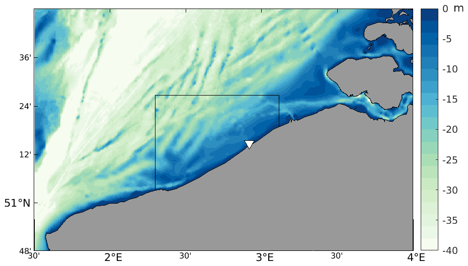
Figure 1 Bathymetry (m) of the southern North Sea. The black square shows the region used in this study and the white triangle shows the position of the validation station RT1.

This work is organized as follows: Sect. 2 describes the region of study, the satellite data, and the in situ data used. This section is followed by a description of the methodology to produce super-resolution data using DINEOF (Sect. 3). The results, including the validation and an assessment of the scales resolved by all of the data sources, are presented in Sect. 4. A description of small-scale variability in the southern North Sea using the super-resolution dataset is presented in Sect. 5, and we conclude this work in Sect. 6.

2 Data used

2.1 Study area

This study focuses on dynamics and optically complex waters in the Belgian coastal zone (BCZ). The BCZ is a relatively shallow (< 50 m) well-mixed shelf sea connected to the North Sea in the north and the English Channel in the west (Ruddick and Lacroix, 2006). It is characterized by a relatively high suspended sediment concentration, with a gradient from several hundreds of grams per cubic metre near the shore to < 1 g m⁻³ in the offshore waters, which is inversely related to the bathymetry (Nechad et al., 2009, 2011; Neukermans et al., 2012). Strong tidal currents and the tidal resuspension of sediments are the main causes of the high turbidity in the nearshore area (Fettweis and Van den Eynde, 2003; Fettweis et al., 2007). Annually recurring phytoplankton blooms are observed in spring and summer. These blooms are generally composed of diatoms and Phaeocystis globose (Lacroix et al., 2007). In recent years, blooms have been occurring earlier, likely in response to sea surface temperature increases and changes in nutrient outputs (Desmit et al., 2020; Alvera-Azcárate et al., 2021b). The water type is turbid coastal to turbid coastal with a high organic content. The water at Research Tower 1 (RT1) near Oostende (51.24643° N, 2.91933° E), used in the validation of the various datasets in this work, is turbid with tidal variability and with an occasional outflow from the port of Oostende (Belgium) reaching the site.

2.2 Satellite data

The ocean colour satellite products used in this study are generated following the methodology applied in the high-resolution Copernicus Marine Service using a multi-algorithm approach which aims to combine the best-suited algorithms for different water types. The year 2020 was chosen for the test period, as this year has the largest unbroken time series of independent in situ data at the Oostende RT1 station used to validate the super-resolution DINEOF product and its potential to capture the coastal turbidity dynamics. To facilitate Sentinel-2 and Sentinel-3 product generation, the processor is fully automated and set up in the DIAS cloud environment CREODIAS (https://creodias.eu/, last access: 30 March 2025). This processor starts from L1C and L1 data for Sentinel-2/MSI and Sentinel-3/OLCI respectively and combines atmospheric correction processing (C2RCC + ACOLITE dark-spectrum fitting), IDEPIX pixel classification, ocean colour algorithm application, and product quality control (e.g. glint flagging or bottom reflection flagging) to provide analysis-ready data layers (ARDLs), i.e. chlorophyll (CHL), turbidity (TUR), and suspended particulate matter (SPM). A schematic overview of the different processing steps taken is provided in Fig. 2.

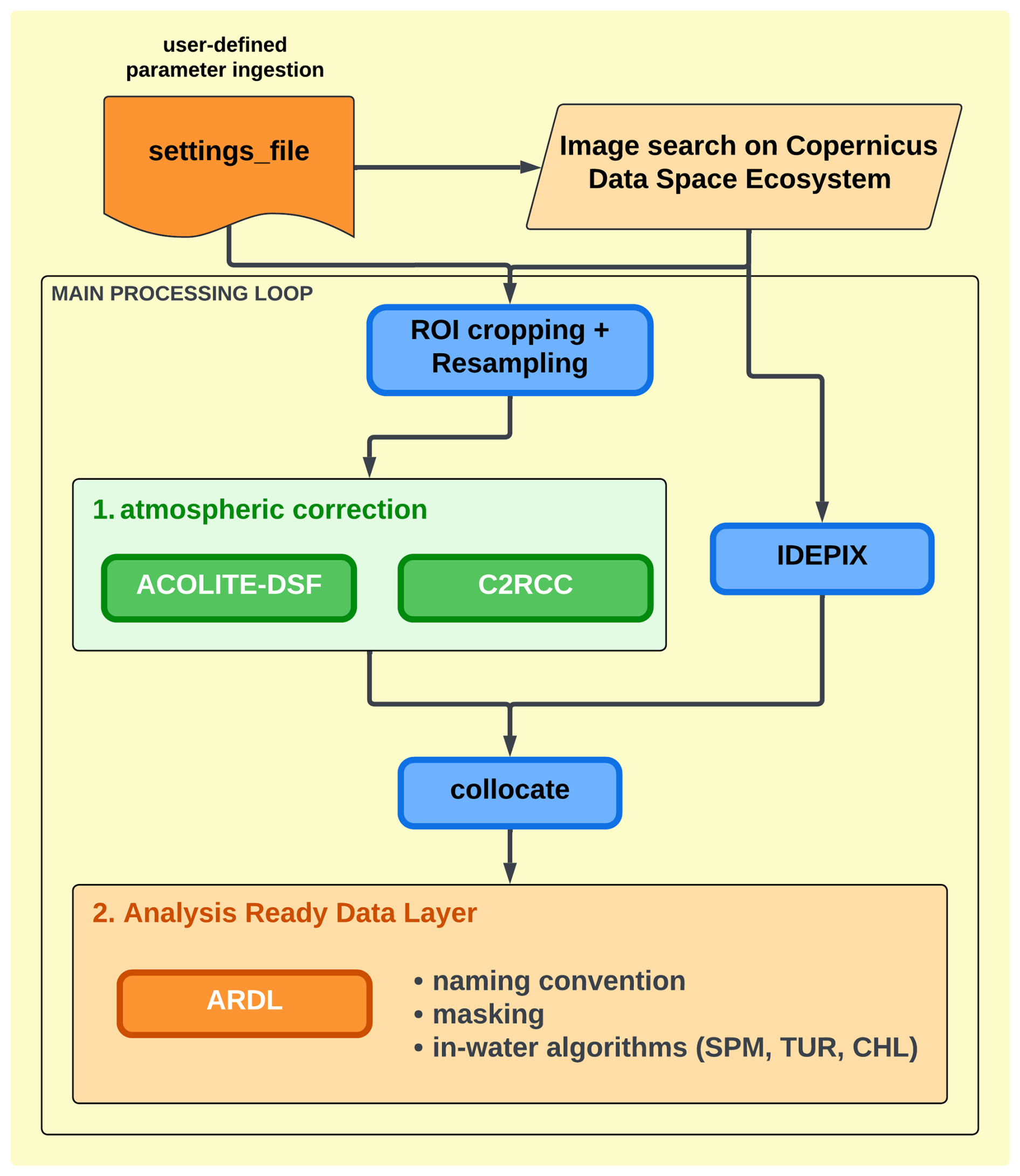
Figure 2 Processing steps applied to derive the L2 ARDL products used for both the Sentinel-2/MSI and Sentinel-3/OLCI sensors. The processor combines the atmospheric correction algorithms ACOLITE and C2RCC, uses SNAP to crop and resample the data to the region of interest, and runs IDEPIX for pixel classification, after which all the intermediate layers are collocated together to the required resolution. In the final step, the in-water ocean colour products are generated using specialized algorithms.

2.2.1 Remote sensing reflectance and pixel classification

In order to obtain high-quality remote sensing reflectance (RRS) spectra for a large number of pixels while maintaining the ability to handle both atypical water conditions and challenging atmospheric conditions, the atmospheric correction algorithms ACOLITE/DSF (https://github.com/acolite/acolite, last access: 30 March 2025) and C2RCC (https://c2rcc.org/, last access: 30 March 2025) are combined to process L1C products to L2R (level-2 RRS) products. While both algorithms have their strengths and weaknesses, they each use different approaches to estimate RRS. C2RCC uses an underlying water reflectance model to fit the estimated RRS spectrum to a known form within the boundaries of the training dataset. This method reduces noise in low-RRS situations and provides greater retrieval power in difficult circumstances, such as Sun-glinted and highly absorbing waters. On the other hand, ACOLITE/DSF does not assume a specific water reflectance model, allowing it to return unusual RRS spectra that correspond to optical properties not found in typical water reflectance models. This can complement C2RCC where it is less performant, such as when dredging plumes and unusual algae blooms.

To combine the two approaches, a comprehensive, region-independent, and pixel-based automatic switching scheme is required, along with a technique for achieving a seamless transition between the two algorithms. The C2RCC-to-ACOLITE/DSF pixel-based switching is performed by means of band comparison of the RRS560 and RRS865 products (defined as the green : near-infrared ratio) as provided by the C2RCC processor. The green : near-infrared ratio can be modelled using a logarithmic regression curve which starts as linear for the smaller reflectance values but bends at the point where the saturation of the most sensitive band (i.e. RRS560) occurs. C2RCC pixels which deviate from the logarithmic model are considered erroneous outputs. The ACOLITE/DSF processor has the ability to provide higher RRS ranges compared to C2RCC while being noisier for lower RRS values, thus highlighting the complementary nature of the two approaches. The green : near-infrared ratio value of 45 is selected as the transition point between the C2RCC and ACOLITE/DSF products. To ensure a smooth transition between the different atmospheric corrections, a weighted transition is applied between the green : near-infrared ratio boundaries of 50 and 40 based on the method described by Novoa et al. (2017). The C2RCC-to-ACOLITE/DSF pixel-based switching is described in detail in Van der Zande et al. (2023). Compatibility of the Sentinel-2/MSI products and the Sentinel-3/OLCI products was ensured by applying the identical processing chain to both datasets.

The IDEPIX software (v2.2.10, algorithm update 8.0.3), available as a SNAP (Sentinel Application Platform) processor, is used for pixel classification, including cloud masking, cloud shadow identification, sea ice, floating vegetation, sub-pixel objects (ships, small islands, and rocks), and the land–water distinction taking temporary water bodies (e.g. intertidal areas or lagoons) into account. SNAP is a software package developed by the European Space Agency (ESA) that is designed to process and analyse Earth observation data, particularly from the Sentinel satellites. It provides a common architecture for all Sentinel toolboxes and enables the application of the C2RCC and IDEPIX processors to both Sentinel-2 and Sentinel-3 images.

2.2.2 Turbidity and suspended particulate matter

The SPM and TUR products were generated using the generic multi-sensor algorithm described by Nechad et al. (2010). This algorithm provides the theoretical basis for SPM and TUR as functions of RRS at a single band and provides calibration coefficients for all wavelengths between 520 and 885 nm. It defines a relationship where RRS increases monotonically with SPM or TUR, at first linearly and then tending towards an asymptotic or “saturation” reflectance. This means that RRS becomes insensitive to changes in SPM and TUR, which has led to the development of “switching single band algorithms” (Novoa et al., 2017) using different wavelengths at different SPM concentrations in order to avoid the saturation effect and typically a smooth weighting between two adjacent spectral bands in order to avoid image artefacts. The Novoa et al. (2017) approach is applied to the SPM and TUR products, providing a multi-band SPM and TUR product using two bands (red: 665 nm; near-infrared: 865 nm). An example of the TUR products for the Belgian coastal zone region is provided in Fig. 3, showing good correspondence between the Sentinel-2/MSI and Sentinel-3/OLCI products and providing information at different spatial and temporal resolutions.

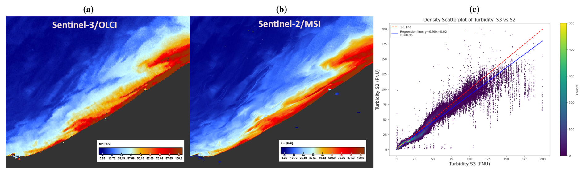
Figure 3 TUR products for 5 April 2020 for the Belgian coastal zone region generated using the multi-sensor processor with Sentinel-3/OLCI (a) and Sentinel-2/MSI (b) source data. Panel (c) shows a density scatterplot of the Sentinel-3 and Sentinel-2 datasets.

2.2.3 Multi-sensor chlorophyll data

In order to assess the small-scale information retained in the final DINEOF reconstructions, an additional test on a larger region has been done using data at 1 km resolution. The aim is to create a degraded 5 km resolution dataset from the initial data and to compare the DINEOF results to the initial, non-degraded dataset. This scale assessment is described in Sect. 4.3. Daily chlorophyll data at a spatial resolution of 1 km, obtained from the level-3 multi-sensor cmems_obs-oc_atl_bgc-plankton_my_l3-multi-1km_P1D product from CMEMS (Copernicus Marine Service, https://doi.org/10.48670/moi-00286), are used in this analysis. This product includes data from different sensors (SeaWIFS, MERIS, MODIS-Aqua, MODIS-Terra, VIIRS-SNPP, VIIRS-JPPS1, OLCI-S3A, and OLCI-S3B) and covers the whole North Sea area (48.46–55.96° N, −1.64–6.15° E). We have extracted data from 1 February to 1 November 2022 in order to have a long time series of data, avoiding January and December, which have low-light conditions and prevent the calculation of ocean colour variables at the higher latitudes of the domain. The choice of year was simply to avoid 2020, which is used in the other tests. A total of 271 images are available, with an average amount of missing data, due to cloud cover and quality control, of 38.17 %.

2.3 In situ data

The RRS products were validated using the Pan-and-Tilt Hyperspectral Radiometer system (PANTHYR, Vanhellemont, 2020; Vansteenwegen et al., 2019) for the period 2019–2022. An autonomous PANTHYR system was deployed at RT1 near Oostende (51.24643° N, 2.91933° E). The PANTHYR system has two TriOS RAMSES radiometers mounted on a pan-and-tilt head, one for upwelling and downwelling spectral radiances and one with a cosine collector to measure spectral irradiance, enabling us to determine the RRS signal. The PANTHYR system measures autonomously every 20 min at programmed relative azimuth angles to the Sun. In the present study, measurements were made at a 270° azimuth angle. Because of the hyperspectral measurements, one significant advantage of the PANTHYR datasets when compared to AERONET-OC and typically used to validate ocean colour satellites (Zibordi et al., 2009) is that the hyperspectral instrument permits the validation of all MSI and OLCI VNIR bands within the 400–900 nm range, including several near-infrared bands not available with the AERONET-OC instrument. RRS data were finally convolved to the relative spectral response functions of the MSI and OLCI instruments on Sentinel-3 A and B and Sentinel-2 A and B.

Match-ups for the PANTHYR stations were extracted from locations slightly to the east (RT1_shifted; 51.24643° N, 2.9206°0 E) of the deployment tower to avoid platform effects such as direct pixel contamination and shadows as well as in-water wakes. For the match-up extraction, a maximum time difference of 2 h between in situ observation and satellite overpass was allowed. However, the high-frequency measurement protocol from the in situ measurement stations resulted in shorter time differences between in situ and satellite observations. The match-up validation protocol described by Bailey and Werdell (2006) was applied to remove erroneous match-ups from the analysis. Macro-pixels of 15 × 15 60 m pixels for Sentinel-2/MSI and 3 × 3 300 m pixels for Sentinel-3/OLCI were extracted from the L2 products. This box allows for the evaluation of spatial stability, or homogeneity, at the validation point. For the satellite data it was required that at least 60 % of the pixels in the defined box be valid (i.e. unflagged) to ensure statistical confidence in the mean values retrieved. The arithmetic mean and standard deviation of the non-masked pixels were determined, enabling the computation of the coefficient of variation (standard deviation divided by the filtered mean). Satellite retrievals with extreme variation between pixels in the defined box (coefficient of variation > 0.15) were excluded from the match-up analysis.

3 Methodology

3.1 DINEOF

DINEOF (Beckers and Rixen, 2003; Alvera-Azcárate et al., 2005) is used to calculate the reconstruction of the data and to enhance the resolution of the combined Sentinel-2 and Sentinel-3 dataset. It computes the missing data from a three-dimensional dataset by calculating a truncated empirical orthogonal function (EOF) basis. These EOFs are calculated increasingly (starting from one until the optimal number of EOFs is found) and iteratively until a convergence is reached, and at each iteration the estimate of the missing data is updated using the latest EOF modes. About 3 % of valid data (in the form of clouds, following Beckers et al., 2006) are masked at the beginning of the procedure, and these data are used to determine the number of EOFs that minimize the reconstruction error (in terms of its root mean square error or RMSE). When three consecutive EOFs provide an increasingly higher RMSE, the procedure is stopped and the final reconstruction is performed with the optimal number of EOFs determined by this cross-validation.

In addition to the reconstruction of missing data in several variables (e.g. sea surface temperature, Alvera-Azcárate et al., 2005; chlorophyll, Alvera-Azcárate et al., 2021b; turbidity, Alvera-Azcárate et al., 2015; salinity, Alvera-Azcárate et al., 2016; and multi-variate reconstructions, Alvera-Azcárate et al., 2007), DINEOF has been used to detect outliers in satellite data (Alvera-Azcárate et al., 2012, 2015) and shadows in high-spatial-resolution satellite data (Alvera-Azcárate et al., 2021a). DINEOF has therefore shown that it can perform a wide range of analyses of satellite data with the aim of improving their quality and completeness.

3.2 Generation of super-resolution data

In order to obtain a super-resolution reconstruction from the combination of Sentinel-3/OLCI and Sentinel-2/MSI data mentioned in Sect. 2, the initial gappy matrix is prepared as follows: Sentinel-2 data are used preferentially and, on days with no Sentinel-2 coverage, Sentinel-3 data, interpolated at the Sentinel-2 spatial resolution of 60 m, are used. The matrix therefore consists of a mixture of Sentinel-2 and Sentinel-3 data. The interpolation of Sentinel-3 data onto the Sentinel-2 grid using the nearest-neighbour method is done to preserve the size of the matrix, which has to be constant in order to be used in DINEOF and to determine the spatial resolution of the final dataset, but no gain in resolution is made at this step.

On days when Sentinel-2 and Sentinel-3 data are available, only Sentinel-2 data are used. We could slightly increase the spatial coverage on these days by combining both data streams, but we found the increase to be very small, since cloud distribution does not change substantially between the Sentinel-3 and Sentinel-2 passes. In addition, depending on the tidal currents, the difference in turbidity between the two satellite passes can be quite high, and this can lead to discontinuities between both estimates, which in turn can be retained in the final dataset. We have therefore decided to avoid this problem by using a unique data source on a given day.

The initial dataset with the combined Sentinel-2 and Sentinel-3 data has 210 time steps, of which 63 % are Sentinel-3 data and 37 % are Sentinel-2 data. Days with overly high cloud coverage (more than 98 % missing data over the study region) are not used, which brings the final size to 163 d, distributed from 18 January to 17 December 2020.

The combined dataset is fed into DINEOF as a unique matrix. As DINEOF does not re-grid the data, it is important that the initial data are already gridded to the final grid that we want to obtain (i.e. the high-spatial-resolution grid). Through the EOF basis calculation, the high spatial information of Sentinel-2 is extracted by the EOFs, and this information is then projected into the final dataset by the EOF basis, effectively increasing the spatial resolution of the initial dataset.

4 Results

4.1 Super-resolution data

Super-resolution DINEOF (Sect. 3) has been applied to the turbidity data in the Oostende region described in Sect. 2. The initial matrix has 45 % of missing data. DINEOF was applied to the combined Sentinel-2 and Sentinel-3 data for 2020, and 23 EOFs were retained as optimal for the reconstruction, with a cross-validation error of 1.4 FNU. The size of the matrix was 946 × 789 × 210 (longitude, latitude, and time), and the DINEOF run took 8 h to complete (on an Intel Core i9-10900X CPU at 3.70 GHz). The only two optional parameters to set in DINEOF are related to the filtering of the temporal covariance matrix (Alvera-Azcárate et al., 2009) and were fixed to α=0.01 (the amplitude of the filter) and n=3 (the number of iterations of the filter). These result in a filter of about 1.1 d. As shown in Alvera-Azcárate et al. (2009), the use of this filter can result in more EOFs being retained as optimal, which in turn results in a higher variability in the final results. Several tests were performed for values α=0.01 to α=0.1 and n=1 to n=10, and the combination that maximized the number of EOFs was retained. The first three EOFs explain 59.04 %, 25.73 %, and 3.74 % of the total variability of the dataset, and the 23 EOFs retained explain the total of 97.9 % of the variability. When analysing the spatial and temporal structures of these EOFs, we can observe the influence of small-scale variability contained in them. The first EOF mode (Fig. 4) displays an inshore–offshore gradient on which more turbid waters are found in the nearshore region. An increasing turbidity along the coast is found towards the region of the Scheldt estuary. The factors responsible for the higher turbidity in this region have been attributed to tides and meteorological conditions (Fettweis and Van den Eynde, 2003) and show peaks in January, April, June, and September–October 2020. This mode shows large-scale processes, and there is no apparent small-scale variability present in the first spatial EOF.

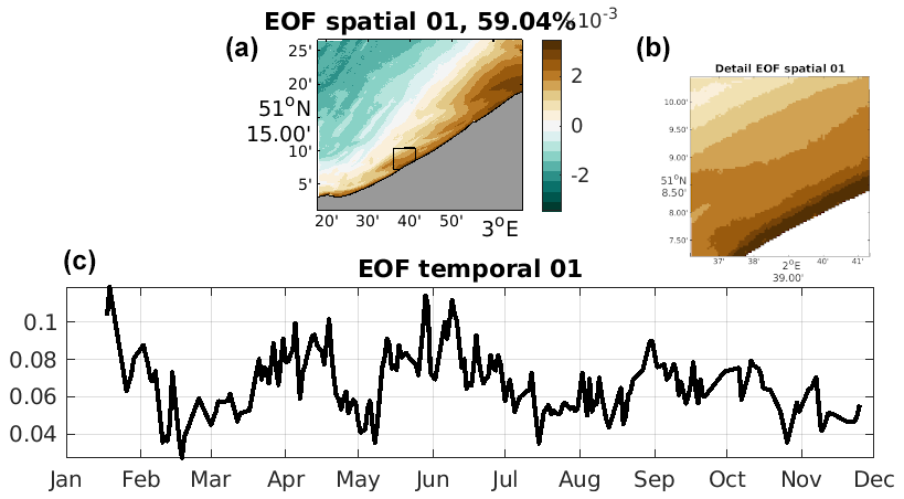
Figure 4 First EOF mode of the 2020 turbidity data obtained by DINEOF. (a) Spatial EOF mode. (b) Detail of the spatial mode in the black square shown in panel (a). (c) Temporal EOF mode.

The second EOF mode (not shown) already displays small-scale spatial variability. We show here the third EOF mode (Fig. 5), which shows a NE–SW gradient with high variability in the temporal mode. In the detailed panel shown in the figure we can also appreciate a thin region along the coast with behaviour opposite to the more offshore waters. Thanks to its high spatial resolution, it has been shown (https://www.esa.int/Applications/Observing_the_Earth/Copernicus/Sentinel-2/Near-shore_phytoplankton_bloom_captured_from_space, last access: 30 March 2025) that Sentinel-2 is able to capture small-scale variability that was previously unknown, i.e. a variability that has been captured by the EOF basis to produce the final, super-resolution datasets that will be shown in this section. The validation of the initial data and the super-resolution reconstruction will be presented in Sect. 4.2.

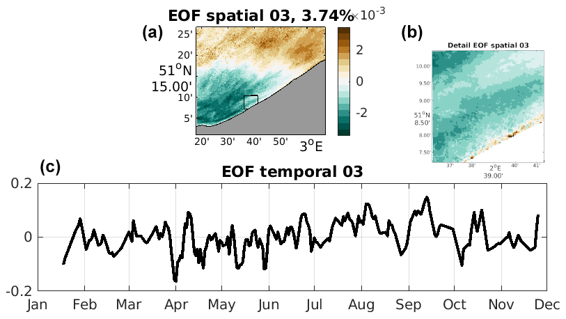
Figure 5 Third EOF mode of the 2020 turbidity data obtained by DINEOF. (a) Spatial EOF mode. (b) Detail of the spatial mode in the black square shown in panel (a). (c) Temporal EOF mode.

Figure 6 shows the initial turbidity data on 9 May 2020, a day with, initially, Sentinel-3 data (i.e. low-resolution data). A day with low cloud coverage was chosen in order to show the ability of DINEOF to enhance the spatial resolution. The initial data (Fig. 6a) show a series of high- and low-turbidity regions, a pattern that is due to the presence of sandbanks close to the Belgian coast. The changes in depth in this region induce large differences in turbidity from day to day. High-turbidity values in the east of the figure are due to the Scheldt–Rhine plume, which is located to the east of the domain. The reconstructed image (Fig. 6b) reproduces all of these features, as also seen in the contours added to this figure. A north–south transect is also included in the figure to show the small-scale variability that has been included in the reconstruction. The initial data (in blue in Fig. 6c) do not contain this small-scale variability and instead present a step-like nature due to the low spatial resolution of the initial dataset. This step-like variability is absent from the final, super-resolution data, which instead show smaller-scale variability. A percentage change map is also included, showing differences between the initial and final products over the whole domain, with a dominance of along-shore structures following the sandbanks present in the region that cause changes in turbidity. Most of the changes between the initial and final products therefore affect the structures of these sandbanks and other high-turbidity features offshore. The difference in resolution between the initial and final products is also responsible for the changes observed in this figure. Sentinel-2 data have a 60 m resolution, Sentinel-3 data have a 300 m resolution, and the DINEOF reconstruction should be between these two. The sandbanks have different TUR intensities in all the products, and since they present sharp gradients this will be felt in the percentage change map.

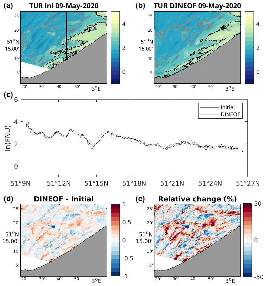
Figure 6 (a) Initially cloudy data at 300 m resolution on 9 May 2020 (logarithmic scale; ln(FNU)). (b) DINEOF run of the mixed Sentinel-2 and Sentinel-3 dataset at 60 m resolution (logarithmic scale). Grey contours in panels (a) and (b): 1.5 ln(FNU); black contours: 3 ln(FNU). (c) North–south transect for the two datasets (blue: initial data at 300 m; black: super-resolution DINEOF reconstruction). (d) Difference between the initial and reconstructed data. (e) Percentage difference map.

Figure 7 shows a similar reconstruction to Fig. 6 but this time for a date on which Sentinel-2 data are available (i.e. high-spatial-resolution data). This example shows that the variability of the super-resolution DINEOF reconstruction is similar to that of the initial dataset, and there is only a limited amount of variability lost with the analysis, mostly in regions with low-turbidity values (Fig. 7c). The presence of high-turbidity regions caused by the presence of sandbanks is also visible in this image, and a sharp inshore–offshore turbidity gradient can be seen that is retained well by the reconstruction. The contours in both images show the small-scale variability retained in the reconstruction. Turbid waters in the easternmost part of the domain, close to the Scheldt estuary and the shallowest region of the domain, can also be seen. The percentage change map in this figure shows smaller-scale features, i.e. long and thin structures in an along-shore direction, showing that the turbidity around the sandbanks and in offshore high-turbidity features is being modified between the initial and final datasets. Again, the difference in resolution between the different initial products is reflected in the representation of sharp turbidity gradients in the final product.

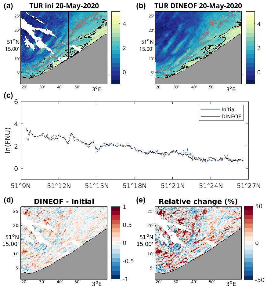
Figure 7 (a) Initially cloudy data at 60 m resolution on 20 May 2020 (logarithmic scale; ln(FNU)). (b) DINEOF run of the mixed Sentinel-2 and Sentinel-3 dataset at 60 m resolution (logarithmic scale). Grey contours in panels (a) and (b): 2 ln(FNU); black contours: 3 ln(FNU). (c) North–south transect for the two datasets (blue: initial data at 60 m; black: super-resolution DINEOF reconstruction). (d) Difference between the initial and reconstructed data. (e) Percentage difference map.

The results shown so far are from images that have good data coverage, but DINEOF also provides super-resolution data on days with high cloud coverage. Two examples in the Supplement show the reconstruction on a day with almost no initial data (Fig. S1) and a day with a high amount of noise in the initial data (Fig. S2). On days with almost no data (Fig. S1 on 12 April 2020), DINEOF is still able to provide a reconstruction with good spatial variability. Reconstruction of the turbidity's spatial distribution on days with high amounts of missing data is possible because of the three-dimensional nature of DINEOF, which exploits the spatio-temporal coherence of the data and enhances temporal correlations (Alvera-Azcárate et al., 2009). The accuracy of the reconstruction can however be affected when persistent clouds obscure a specific region for several days (e.g. Alvera-Azcárate et al., 2005; Zhao et al., 2024). The method proposed by Beckers et al. (2006) would allow us to obtain a pixel-by-pixel estimation of the reconstruction error variance and can be used to assess the influence of persistent cloud cover on the final result.

At some moments, there can be outliers or noise in the initial dataset despite the strong quality controls applied to the data, as in Fig. S2. The fact that DINEOF uses a truncated EOF basis to compute the missing data results in a partial loss of variability. However, this truncated EOF basis guarantees that the presence of outliers will not influence the overall quality of the reconstruction. As an example, in Fig. S2 we can see the turbidity on 28 May 2020, with a region in the northern part affected by the presence of noisy data. These are probably due to undetected thin clouds. The north–south transect shows that the variability of these data far exceeds the normal variability expected for the region. The DINEOF super-resolution results provide a reduced amount of noise and an improved quality of the final product while still providing an accurate depiction of small-scale variability.

4.2 Validation

Using the in situ data described in Sect. 2.3, a quality assessment of the initial data and the DINEOF results has been realized. Figure 8 shows the RRS match-ups between Sentinel-2/MSI and the PANTHYR in situ instrument installed on RT1. The metrics used are described in the Appendix. In the considered deployment period between 11 December 2019 and 1 August 2023, 528 MSI L1C images were available for processing with 53 match-ups with the PANTHYR instrument, which passed the quality flagging of the individual atmospheric corrections (i.e. ACOLITE/DSF and C2RCC), IDEPIX quality flagging, and match-up quality flagging. When using the merged approach for atmospheric correction, the best-performing bands are 490, 560, 665, and 704 nm, which are typically used for retrieval of turbidity and turbid-water chlorophyll a. For these bands the median absolute percentage error (MAPE) ranges between 9.88 % and 17.20 %.

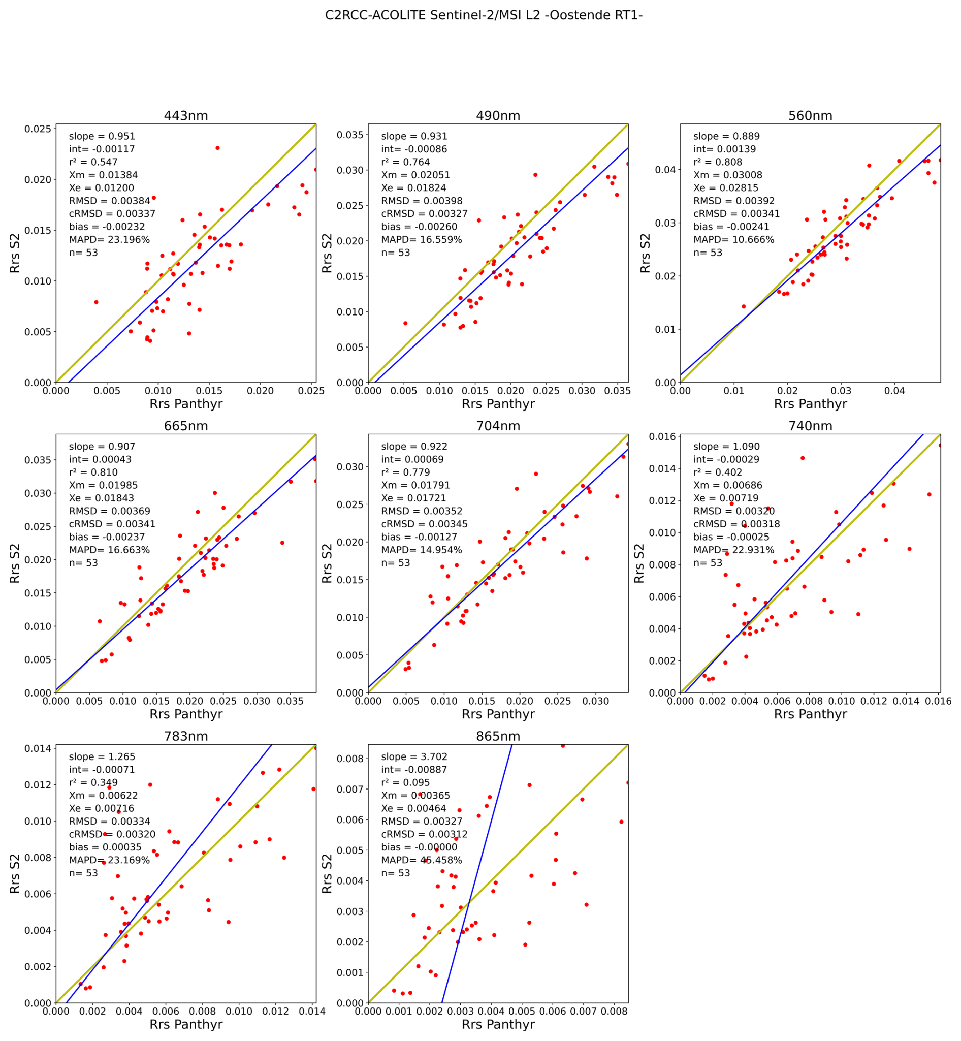
Figure 8 Validation of RRS for Sentinel-2/MSI data. Hyperspectral in situ stations from the HYPERNET network in Oostende (Belgium) were used.

Figure 9 shows the RRS match-ups between the Sentinel-3/OLCI and PANTHYR instruments installed on RT1. In the deployment period between 11 December 2019 and 1 August 2023, 2334 OLCI L1FR images were available for processing with 168 common match-ups with the PANTHYR instrument, which passed the quality flagging of the individual atmospheric corrections (i.e. ACOLITE/DSF and C2RCC), the IDEPIX quality flagging, and the match-up quality flagging. For the merged approach of atmospheric correction, the best-performing bands are 443, 490, 560, 665, and 709 nm, which are typically used for retrieval of turbidity and turbid-water chlorophyll a. For these bands the MAPE ranges between 10.74 % and 19.00 %.

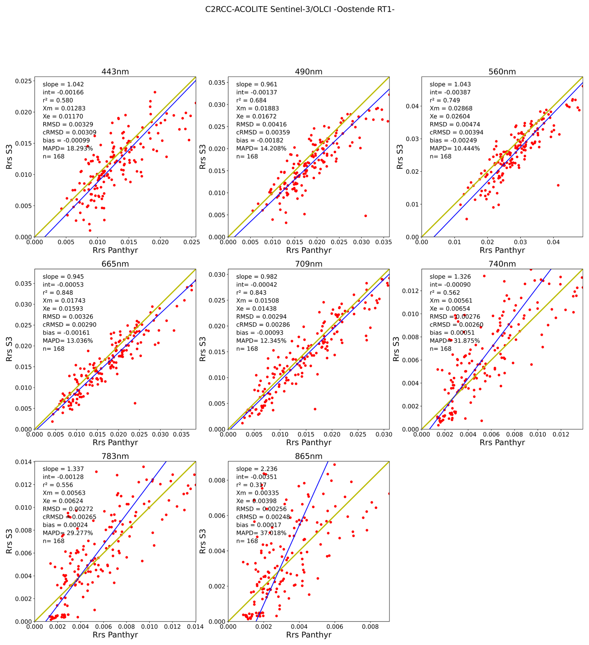
Figure 9 Validation of remote sensing reflectance (RRS) for Sentinel-3/OLCI data. Hyperspectral in situ stations from the HYPERNET network in Oostende (Belgium) were used.

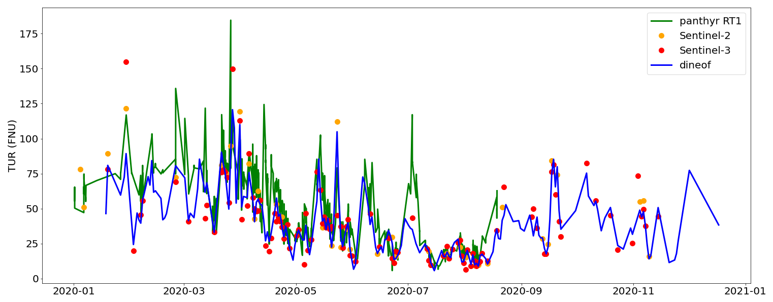
Figure 10 Turbidity time series for 2020 at the RT1 HYPERNET station generated using the in situ hyperspectral PANTHYR data (green line), the Sentinel-2 satellite data (orange dots), the Sentinel-3 satellite data (red dots), and the gap-filled DINEOF super-resolution satellite product (blue line).

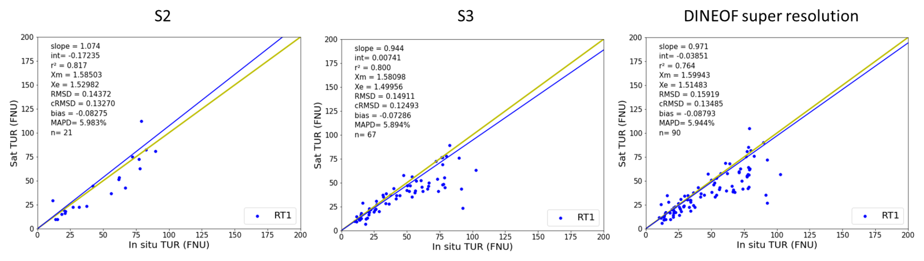
Figure 11 Match-up results of the daily Sentinel-2, Sentinel-3, and DINEOF super-resolution TUR products against in situ observations obtained from the autonomous PANTHYR system at the RT1 station in the Belgian coastal zone.

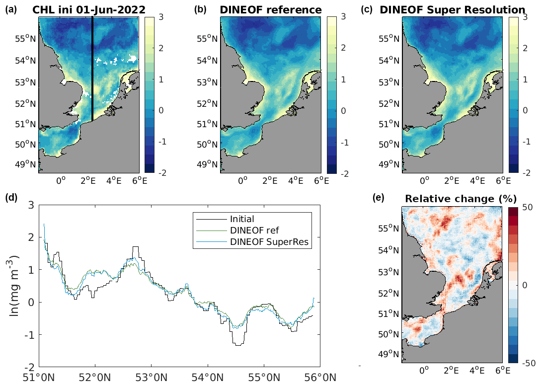
Figure 12 (a) Initially cloudy data with 5 km resolution on 1 June 2022. (b) DINEOF reconstruction of the 1 km data (reference run). (c) DINEOF run of the mixed dataset. (d) North–south transect for the three datasets (black: initial data at 1 and 5 km; green: reference run at 1 km; blue: super-resolution run). (e) Percentage difference map between the initial data and the DINEOF estimate. The data are on a logarithmic scale.

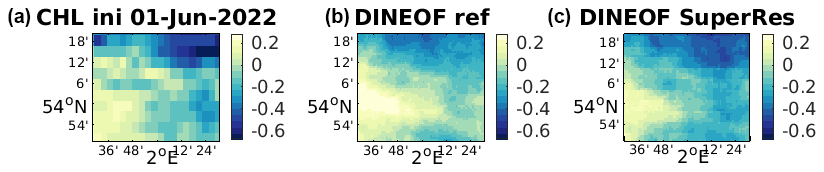
Figure 13 Example of super-resolution DINEOF reconstruction. (a) Initial data downgraded to 5 km spatial resolution on 1 June 2022. (b) Reconstruction of the reference run at 1 km spatial resolution. (c) Reconstruction of the 5 km data with DINEOF using the mixed 1 and 5 km dataset. The data are on a logarithmic scale.

The accuracy of the DINEOF super-resolution products was validated for the Belgian coastal zone region by using the hyperspectral in situ dataset from the autonomous PANTHYR system deployed at RT1 near Oostende to generate an in situ turbidity product which was directly compared with the satellite-derived turbidity products. This resulted in a turbidity time series with a temporal resolution of 20 min when daylight was available. The in situ turbidity product was generated with the same algorithm as used for the satellite products. Figure 10 shows the turbidity time series for 2020 overlaying the in situ data, the Sentinel-2 and Sentinel-3 turbidity products, and the final super-resolution DINEOF gap-filled product showing that the DINEOF product is able to capture the in situ turbidity signal between March and September. In January and February the DINEOF product shows slightly lower values, which can be caused by the fact that in those months the availability of cloud-free satellite products from Sentinel-2 and Sentinel-3 is very low. In situ observations for the period September–December were unavailable as the PANTHYR system was taken down for maintenance.

An objective intercomparison was achieved through a match-up analysis. The match-up validation protocol described by Bailey and Werdell (2006) was applied to remove erroneous match-ups from the analysis based on macro-pixels of 3 × 3 pixels from the satellite turbidity products. Figure 11 shows the results of the match-up analysis for Sentinel-2, Sentinel-3, and the gap-filled DINEOF super-resolution products. These graphs show that the Sentinel-2 and Sentinel-3 products are in good agreement with the in situ observations, with mean average percentage differences of around 6 %. The temporal frequency of Sentinel-3 overpasses over the region of interest results in more than 3 times more match-ups. Considering the DINEOF super-resolution match-ups, this number of match-ups is increased by another 34 %, with very similar statistics compared to the Sentinel-3 match-ups, thus showing DINEOF's ability to retain the turbidity information provided by the source products. We do see a slight underestimation of the turbidity values by both satellites, especially for higher values (turbidity > 50 FNU). Further inspection indicates that this underestimation mostly happens in the winter months (January–February), probably due to the high cloud cover (data not shown).

4.3 Scale assessment

In order to determine which scales are reconstructed in the super-resolution DINEOF approach, a test using the multi-sensor satellite chlorophyll data at 1 km spatial resolution described in Sect. 2.2.3 was performed. These data are downscaled to 5 km using a nearest-neighbour interpolation (to avoid smoothing the data). Following the same procedure as with the combined Sentinel-2 and Sentinel-3 turbidity dataset, we intercalate the 1 km data and the 5 km data. The ratio of this mixed dataset is one high-resolution image (at 1 km) to every three low-resolution images (at 5 km) in order to mimic the ratio of the Sentinel-2 and Sentinel-3 combination used in the previous section. This allows us to compare the scales reconstructed on this dataset with the initial 1 km data on days when 1 km data and 5 km data were used. In addition, we have made a reference reconstruction of the original, 1 km data so that we can assess how a full high-spatial-resolution reconstruction compares with the mixed-dataset reconstruction.

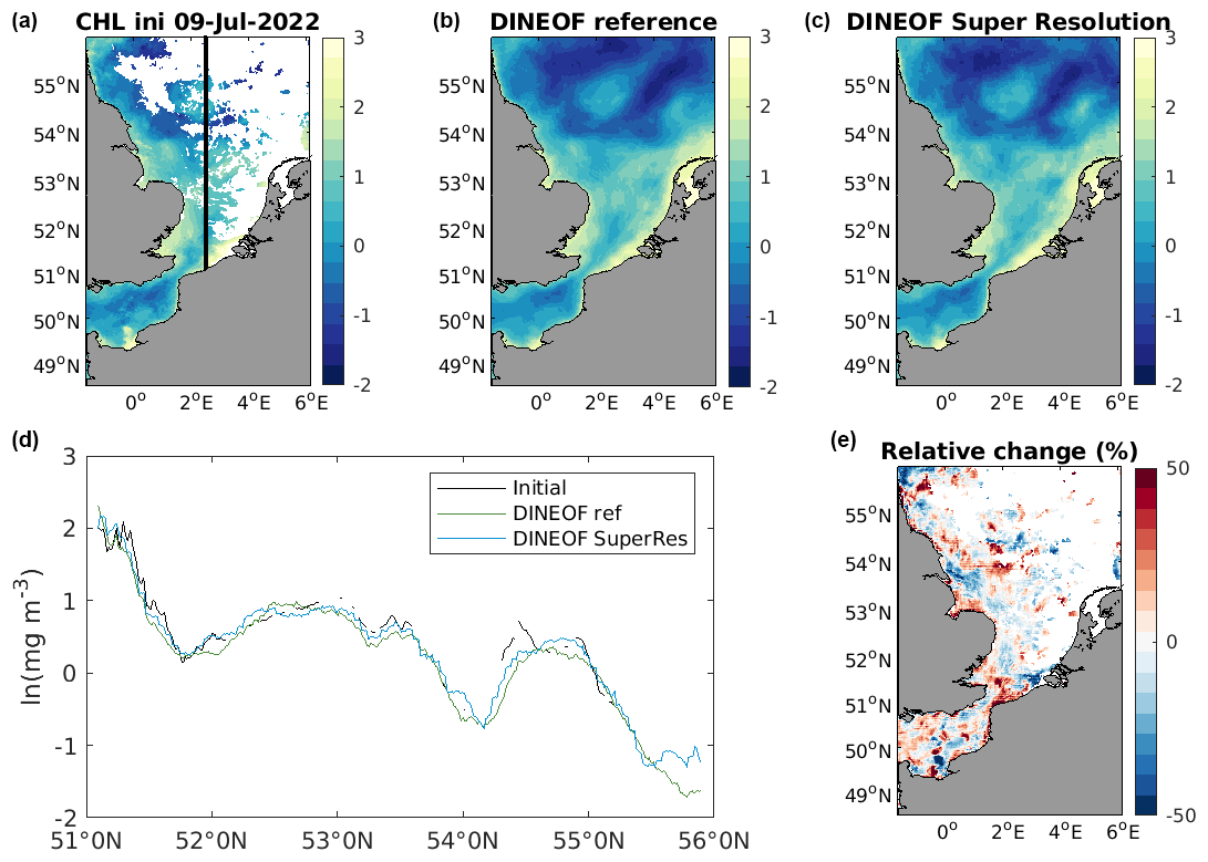
Figure 14 (a) Initially cloudy data with 1 km resolution on 9 July 2022. (b) DINEOF reconstruction of the 1 km data (reference run). (c) DINEOF run of the mixed dataset. (d) North–south transect for the three datasets (black: initial data at 1 and 5 km; green: reference run at 1 km; blue: super-resolution run). (e) Percentage difference map between the initial data and the DINEOF estimate. The data are on a logarithmic scale.

The DINEOF reconstruction of the mixed dataset used 22 EOFs, and an example of the reconstruction is shown in Fig. 12. On this date, 1 June 2022, the initial dataset has a spatial resolution of 5 km. A north–south transect shows that the reconstruction (in blue) is able to increase the variability of the 5 km data to mimic the variability of the reference dataset, which only uses 1 km resolution data (in green). This effectively increases the spatial resolution of the results with respect to the downgraded dataset (in black), which shows a step-like structure. A percentage difference map is also included, which in addition to showing the regions with higher or lower values in the reconstruction (positive or negative percentage values respectively) shows a square pattern that comes from the partial removal of the low-resolution information.

In order to investigate this pattern further, Fig. 13 shows a detail of the reconstruction on 1 June 2022, in which 5 km data are initially present. The super-resolution DINEOF reconstruction (in Fig. 13c) is shown to provide higher spatial resolution than the initial data, similar to what is obtained with the reference reconstruction at 1 km (shown in Fig. 13b), despite the coarse resolution of the initial field. There are some remaining edge effects showing the initial 5 km grid at the super-resolution, but this comes from the choice of nearest-neighbour interpolation. A linear interpolation would avoid such a pattern in the final results, although this would need to be tested.

On a day with 1 km data initially (Fig. 14, 9 July 2022), we can see that the variabilities observed in the north–south transect for the reference run and the super-resolution reconstruction are very similar, showing the ability of the super-resolution approach to retain small-scale variability.

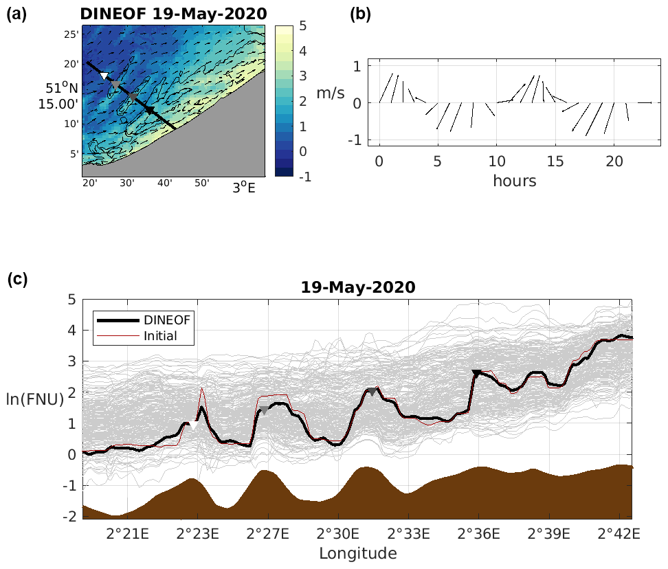
Figure 15 (a) DINEOF super-resolution reconstruction of turbidity on 19 May 2020. The black lines show the 5 and 10 m isobath and the arrows show the surface currents at 10:00. The thick black line shows the transect across the sandbanks in panel (c), and the triangles are positioned at the tops of some of these sandbanks for reference. (b) Hourly surface currents during 19 May at the light-grey triangle. (c) Across-sandbank transect of turbidity. The light-grey lines show all the DINEOF 2020 data, the thick black line shows the 19 May turbidity, and the triangles are shown to ease comparison with panel (a). The dark-red line shows the initial turbidity data, and the bathymetry is shown in brown.

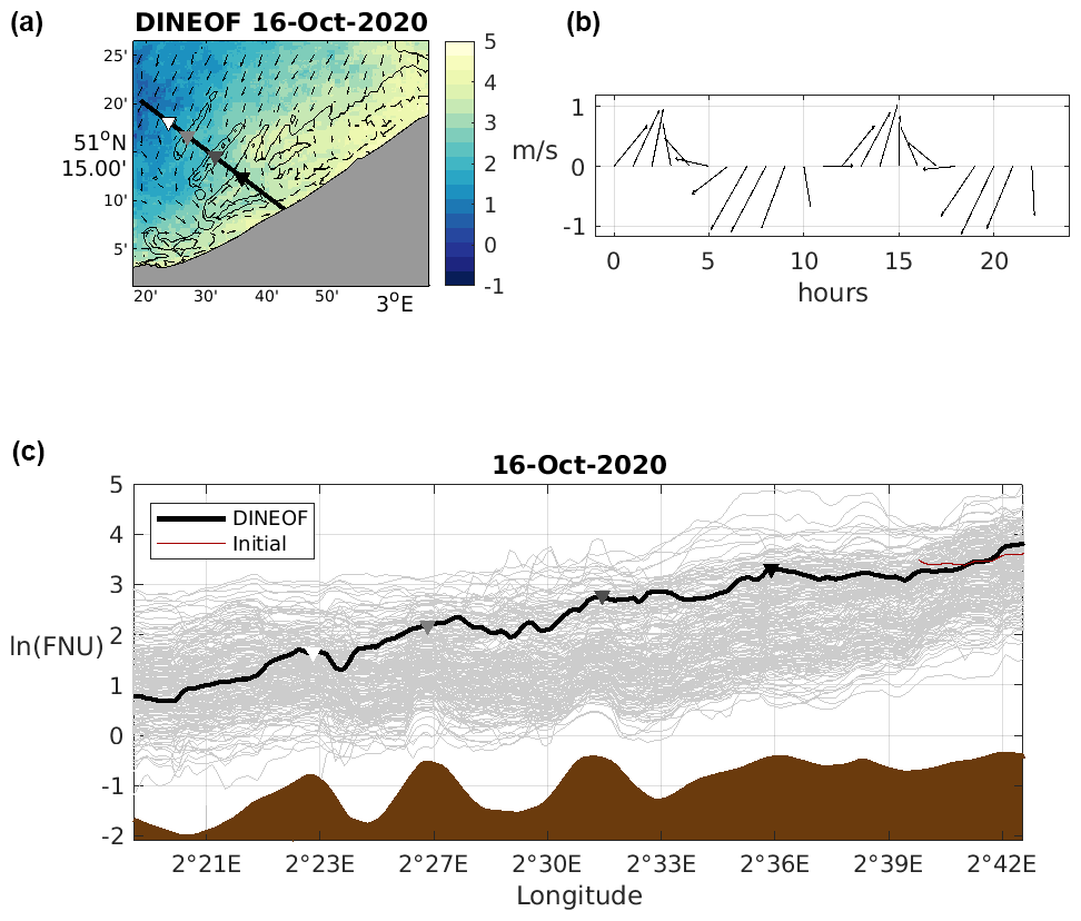
Figure 16 (a) DINEOF super-resolution reconstruction of turbidity on 16 October 2020. The black lines show the 5 m and 10 m isobath and the arrows show surface currents at 10:00. The thick black line shows the transect across the sandbanks shown in panel (c), and the triangles are positioned at the tops of some of these sandbanks for reference. (b) Hourly surface currents during 16 October at the light-grey triangle. (c) Across-sandbank transect of turbidity. The light-grey lines show all the DINEOF 2020 data, the thick black line shows the turbidity on 16 October, and the triangles are shown to ease comparison with panel (a). The dark-red line shows the initial turbidity data, and the bathymetry is shown in brown.

5 Sub-mesoscale variability in the Belgian coastal zone

The super-resolution data obtained in this work allow us to analyse the variability of turbidity at the sub-mesoscale in the study region. The river sediments carried out by the Scheldt and the resuspension of bottom sediments at the along-shore sandbanks are the two major contributors to the small-scale variability of turbidity in this region.

Sandbank-induced high-turbidity patterns on the Belgian coast are influenced by the topography, and horizontal water movement due to tidal currents results in rapid particle deposition outside these shallow environments. As a result, turbidity is often high inside the sandbank region and up to a depth of about 10 m, as observed for example in Fig. 15. We use hourly surface currents obtained from Legrand and Baetens (2021) to assess their influence on the turbidity distribution. The intensity of currents and their direction in the hours preceding the time of the satellite pass have a large influence on the average turbidity values over the region, like on 16 October (Fig. 16), which presents a similar tidal phase to 19 May (top right image) but with stronger currents, resulting in an overall higher turbidity over the whole region.

Figures 15c and 16c show that there is an overall decreasing turbidity in the offshore direction, with similar variability at all depths. The effect of the presence of sandbanks on the resuspension of turbidity is also visible in these images, with regions of higher turbidity corresponding to the presence of these sandbanks. During weak water current periods (Fig. 15), the effect of the sandbanks on water turbidity is seen clearly, with sediments depositing in the deeper, inter-sandbank regions. During strong water current periods (Fig. 16), turbidity is higher everywhere, and the effect of the bathymetry is less evident.

The sandbank-induced high-turbidity patterns in Fig. 15 are about 2 km wide. Temporal scales of the resuspension–deposition processes are mainly determined by tidal currents. It is therefore not possible to observe these processes with satellite data, as they only offer one estimate per day and variations at smaller scales are therefore not measured. Fettweis et al. (2023) showed that, in regions with strong tidal regimes, such as the Belgian coast, the daily sampling from satellites is not enough to capture the variability in the deposition–resuspension cycles caused by tidal currents. Satellite data lack the temporal frequency needed to assess the variability of turbidity at the sandbanks through time, but they provide a relevant tool for analysing the spatial variability at a high spatial resolution.

6 Conclusions

There are several satellite datasets monitoring ocean colour globally, but each of them has different spatial, temporal, and spectral characteristics. It is therefore necessary to develop approaches that allow us to use these data streams in a synergistic way. In the case of coastal studies, there is also a need to work at the highest spatial resolution possible in order to capture the variability that is typical of these regions. All ocean colour satellite sensors are affected by the presence of clouds, and hence these approaches also need to interpolate missing data.

In this work, we have shown an approach for obtaining super-resolution cloud-free satellite data using DINEOF. A combination of Sentinel-2 and Sentinel-3 data representing turbidity on the Belgian coast has been used, and the results show that, working on a combined dataset of Sentinel-2 and Sentinel-3 data, we are able to retain most of the spatial variability present in Sentinel-2 data and to increase the spatial variability of the Sentinel-3 data in order to mimic the Sentinel-2 spatial resolution. The results have been validated using independent in situ data, and the ability of DINEOF to increase the spatial resolution has been validated with a chlorophyll dataset covering the whole of the North Sea. This last example demonstrated that DINEOF is able to recover high-spatial-resolution information, as compared to the original, high-resolution data that were hidden from the analysis. The approach has been tested for different regions (the southern North Sea and Belgian coast in this work) and variables (turbidity and chlorophyll concentration) and can be applied to any other region and variable.

Data with a high spatio-temporal resolution allow us to study small-scale variability in coastal regions, which has been shown in this paper through the influence of sandbanks on the turbidity distribution of the Belgian coast. Variables like turbidity or chlorophyll concentration can vary abruptly in a few metres and within a few hours because of the effect of bathymetry and water currents, for example. Using several satellite datasets to analyse these changes allows for better coverage of the spatio-temporal scales involved. Satellite data however lack the high temporal resolution that would be needed to study the variability of these small-scale features at adequate temporal scales.

Super-resolution satellite products obtained from synergistic use for several satellite data streams are necessary for studying the coastal ocean. The need for high-spatial-resolution data decreases at more offshore locations, and therefore the approach presented in this paper could be applied to a multi-resolution dataset with a higher spatial resolution in the most variable regions. Other future developments include the application of the super-resolution DINEOF approach to variables like sea surface temperature, although the absence of high-spatial-resolution data streams with the necessary accuracy makes this a challenge.