Detection and tracking of carbon biomes via integrated machine learning

In the framework of a changing climate, it is useful to devise methods capable of effectively assessing and monitoring the changing landscape of air–sea CO₂ fluxes. In this study, we developed an integrated machine learning tool to objectively classify and track marine carbon biomes under seasonally and interannually changing environmental conditions. The tool was applied to the monthly output of a global ocean biogeochemistry model at 0.25° resolution run under atmospheric forcing for the period 1958–2018. Carbon biomes are defined as regions having consistent relations between surface CO₂ fugacity (fCO₂) and its main drivers (temperature, dissolved inorganic carbon, alkalinity). We detected carbon biomes by using an agglomerative hierarchical clustering (HC) methodology applied to spatial target–driver relationships, whereby a novel adaptive approach to cut the HC dendrogram based on the compactness and similarity of the clusters was employed. Based only on the spatial variability of the target–driver relationships and with no prior knowledge of the cluster location, we were able to detect well-defined and geographically meaningful carbon biomes. A deep learning model was constructed to track the seasonal and interannual evolution of the carbon biomes, wherein a feed-forward neural network was trained to assign labels to detected biomes. We find that the area covered by the carbon biomes responds robustly to seasonal variations in environmental conditions. A seasonal alternation between different biomes is observed over the North Atlantic and Southern Ocean. Long-term trends in biome coverage over the 1970–2018 period, namely a 1 % to 2 % per decade expansion of the subtropical biome in the North Atlantic and a 0.5 % to 1 % per decade expansion of the subpolar biome in the Southern Ocean, are suggestive of long-term climate shifts. Our approach thus provides a framework that can facilitate the monitoring of the impacts of climate change on the ocean carbon cycle and the evaluation of carbon cycle projections across Earth system models.

1 Introduction

By absorbing roughly 25 % of human-induced carbon emissions annually (Friedlingstein et al., 2023), the global ocean is a critical component of the Earth's climate and has, until now, mitigated the effects of anthropogenic climate change. The ocean's ability to take up CO₂ depends on both physical processes (the “solubility pump”) and biological processes (the “biological pump”) (Sarmiento and Gruber, 2006). The biological soft-tissue pump is driven by the absorption of dissolved inorganic carbon (DIC) by photosynthetic primary producers in the sunlit ocean and by its release into the ocean interior through organic matter remineralization. The solubility pump is driven by various factors, notably ocean temperature, chemistry, and circulation. Sea surface temperature (SST) strongly affects CO₂ solubility, with colder waters capable of absorbing more CO₂ than warmer waters. The chemical composition of seawater also plays a role, with waters characterized by higher alkalinity capable of absorbing higher quantities of CO₂ for a given DIC concentration (Williams and Follows, 2011). Ocean circulation and mixing strongly influence air–sea CO₂ fluxes through their effect on the vertical exchanges of DIC and alkalinity between the ocean surface and its interior.

The processes that govern air–sea CO₂ fluxes display considerable spatial and temporal variability. SST imprints a strong north–south gradient of CO₂ solubility, with colder high-latitude waters exhibiting a higher CO₂ uptake than warmer tropical waters (Williams and Follows, 2011). Overlaid on the solubility-driven gradients, patterns of primary productivity and ocean circulation strongly affect the spatial variability of air–sea CO₂ fluxes. Subpolar regions of high primary productivity act overall as a strong CO₂ sink (Takahashi et al., 2009; Mikaloff Fletcher et al., 2007; DeVries et al., 2023). Exceptions are the subpolar latitudes of the Southern Ocean, the equatorial Pacific, and the eastern boundaries of the ocean basins, where wind-driven upwelling of high-DIC waters and the incomplete utilization of upwelled nutrients make them prone to CO₂ outgassing (Takahashi et al., 2009; Mikaloff Fletcher et al., 2007). High-latitude regions are strongly influenced by sea ice cover, which seasonally hinders the air–sea exchanges of CO₂ and affects surface stratification and primary productivity. The above processes display a substantial seasonal evolution: SST peaks in summer, primary production is highest in spring and summer, and upwelling and vertical mixing are most intense in the cold and wind-swept winter months. Past studies have subdivided the ocean into regions where the air–sea CO₂ flux seasonality is more in phase with SST (“thermal” control) and others where it is more in phase with DIC (“non-thermal” control) (Takahashi et al., 2002; Prend et al., 2022). The oligotrophic subtropical gyres are thermally driven, whereas polar and subpolar regions (characterized by strong biological production and DIC physical transport) are mostly non-thermally driven (Takahashi et al., 2002; Prend et al., 2022). While the seasonal cycle is the strongest source of temporal variation, the natural variability of the climate system also introduces year-to-year changes in the processes governing the CO₂ uptake (Landschützer et al., 2016; Gruber et al., 2023). Prominent examples are the El Niño–Southern Oscillation (ENSO), which modulates the strength of the upwelling in the equatorial Pacific (Feely et al., 2006); the Southern Annular Mode, which modulates the strength of the Southern Ocean upwelling and associated CO₂ outgassing (Lovenduski et al., 2007); and the North Atlantic Oscillation, which modulates the strength of the subpolar North Atlantic deep mixing and overturning circulation with implications for the carbon cycle (Pérez et al., 2013; Patara et al., 2011).

These widely varying environmental conditions have prompted past studies to objectively classify the global ocean into marine biogeochemical biomes. Marine biomes are characterized by coherent physical forcing and environmental conditions, which are representative of distinctive ecosystem structures (Longhurst, 1995; Sonnewald et al., 2020; Oliver et al., 2015). The classification in marine biomes has several applications, such as evaluating and comparing ocean biogeochemical models (Vichi et al., 2011; DeVries et al., 2023), producing air–sea CO₂ flux reconstructions based on sparse observational data (Landschützer et al., 2013), and efficiently interpreting increasingly large datasets produced by Earth system models (Jones and Ito, 2019; Couespel et al., 2024). Recently, biome classification has gone beyond ecosystem applications and explored carbon uptake structures (Fay and McKinley, 2014; Jones and Ito, 2019; Krasting et al., 2022; Couespel et al., 2024). For instance, Fay and McKinley (2014) defined marine biomes based on predefined limits of sea ice concentration, SST, mixed layer depth, and chlorophyll values. These biomes, capable of following dynamical ocean boundaries, have been extensively used to assess and compare air–sea CO₂ fluxes across different models and data products in the recent RECCAP-2 project (DeVries et al., 2023).

Against the backdrop of rapidly evolving machine learning (ML) methods, recent studies have contributed a set of tools for categorizing the global ocean into marine biomes (Landschützer et al., 2013; Jones and Ito, 2019; Sonnewald et al., 2020; Krasting et al., 2022; Mohanty et al., 2023a; Couespel et al., 2024). In their work, Couespel et al. (2024) built target–driver relationships between air–sea CO₂ flux and biogeochemical predictors over a time series and used Gaussian mixture models to cluster the identified temporal associations into carbon regimes. Jones and Ito (2019) also used Gaussian mixture models to segment the ocean surface based on the surface budget of dissolved inorganic carbon, whereas Landschützer et al. (2013) used self-organizing maps to cluster the nonlinear relationships between CO₂ partial pressure and its drivers. Sonnewald et al. (2020) presented the Systematic Aggregated Eco-Province (SAGE) method for constructing eco-provinces, which integrated t-stochastic neighbor embedding (t-SNE) and DBSCAN clustering. The works by Krasting et al. (2022) shed light on Arctic Ocean acidification, where water mass properties were segmented into four clusters using the SAGE method.

When combined with the ability to track the biomes in time, ML-based detection methods could potentially be used to monitor the time evolution of marine biomes under changing climate conditions. For instance, Reygondeau et al. (2020) implemented a regression-based ensemble approach to predict four biomes (subdivided into 56 biogeochemical provinces) in the future. To this end, they used a supervised method based on the location and properties of the 56 biogeochemical Longhurst provinces (Longhurst, 1995). However, due to the strong fluidity of ocean biomes in response to seasonal and interannual changes in environmental conditions, using tracking methods tied to specific locations is not ideal. The challenges in designing ML-based methods for tracking ecosystems over time are numerous. These include (i) the lack of high-quality annotated geoscientific datasets needed for training and validation steps, (ii) building an intricate algorithm to capture the complex spatiotemporal variability within biomes, and (iii) the requirement for considerable computational resources, time, or financial investment, depending on the scale of the available data. Nonetheless, tracking provinces over time can be used to assess and predict transformations in ecosystem functioning and carbon cycle dynamics. Biogeochemical provinces are dynamic entities whose spatial extent and position fluctuate in response to climate variations and are anticipated to be further influenced by forthcoming global climate change (Reygondeau et al., 2020; Couespel et al., 2024). Monitoring these changes over time will detect early signs of ecosystem disruptions, such as ocean acidification (Krasting et al., 2022), allowing for timely intervention and protection measures.

Building upon this motivation, in this study, we built a new strategy capable of detecting and tracking carbon biomes over time, which are defined as regions of consistent relationships between surface CO₂ fugacity (a quantity closely related to CO₂ partial pressure) and its drivers. Instead of applying clustering to the drivers directly, we built multiple localized target–driver relationships between CO₂ fugacity and its predominant drivers (i.e., surface temperature, dissolved inorganic carbon, and alkalinity). Then, we applied agglomerative hierarchical clustering to group similar target–driver connections and detect the carbon biomes through a distribution-aware technique (Mohanty et al., 2023a). Once the clusters are labeled as specific carbon biomes, we employ a simplistic version of a neural network to capture the connections between the labels and the target–driver relationships, enabling the tracking or the prediction of carbon biomes in time. Our approach thus provides a framework that will facilitate monitoring climate change's impacts on the ocean carbon cycle and evaluating carbon cycle projections across Earth system models.

The paper is structured as follows: Sect. 2 describes the global ocean biogeochemistry model used for our analysis and the variables collected from it, the technique to build the target–driver relationships, the application of clustering method to detect the carbon biomes, and the building blocks of the neural network to track the biomes over time. Section 3 elucidates the outcome of the target–driver analysis and the detected clusters, as well as the tracking of the carbon biomes over time. Section 4 discusses our main findings, highlights the study's limitations, and elaborates on potential research ideas for future studies.

2 Methodology

We define a carbon biome as a region characterized by common relationships between carbon uptake and its drivers. Specifically, we use sea surface fugacity of CO₂ (fCO₂) as the target variable and sea surface temperature (SST), surface dissolved inorganic carbon (DIC), and surface alkalinity (ALK) as its drivers. These variables are obtained from a simulation with a global ocean biogeochemistry model (Sect. 2.1). In the face of the intricate and spatially heterogeneous relationship between fCO₂ and its drivers, we construct multiple localized linear relationships within discrete regions, each spanning a 2°×2° dimension, as explained in Sect. 2.2. Subsequently, an agglomerative hierarchical clustering methodology is employed, leveraging the collection of regional multivariate linear regression models. Notably, we employ a distance–variance selection methodology (Mohanty et al., 2023a) tailored to the specifics of our task, thereby automating the detection of clusters on the dendrogram, as outlined in Sect. 2.3. We introduce the application of artificial neural networks in Sect. 2.4 to track the detected carbon clusters. Figure 1 schematically visualizes the entire analytical pipeline, encapsulating the sequential processes.

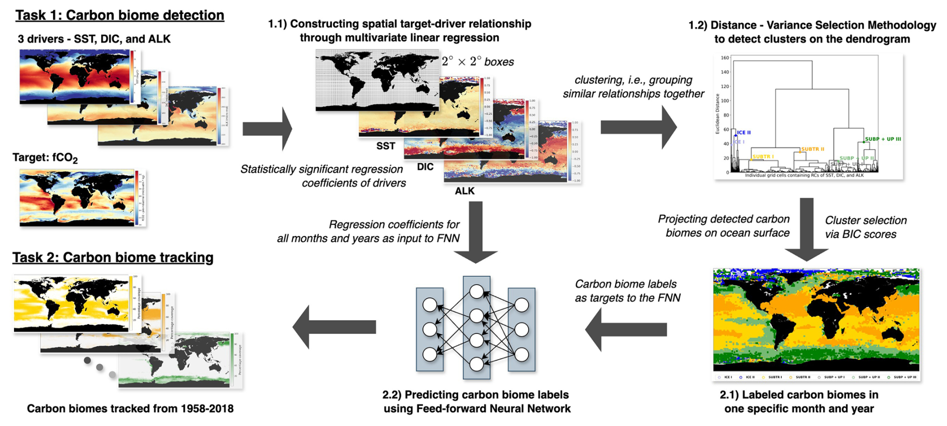
Figure 1 Schematic presentation of the step-by-step approach taken by our study to detect (Task 1) and track (Task 2) marine carbon biomes.

2.1 Ocean model output

We use the monthly output of a global ocean biogeochemistry model composed of the ocean sea ice model NEMO-LIM2 (Madec, 2016) and the biogeochemistry model MOPS (Kriest and Oschlies, 2015; Chien et al., 2022). The model configuration (hereafter called ORCA025-MOPS) is discretized on a global grid having approximately 0.25° horizontal resolution (Barnier et al., 2007) and 46 vertical levels. MOPS simulates the lower trophic levels of the ecosystem and carbonate chemistry using nine biogeochemical tracers (phosphate, nitrate, phytoplankton, zooplankton, detritus, dissolved organic matter, oxygen, DIC, and alkalinity). Calcium carbonate dissolution and production, as well as their effects on alkalinity, are parameterized based on Schmittner et al. (2008). The carbonate chemistry and the air–sea CO₂ exchanges are based on Orr et al. (2017), with an approximate and non-iterative method to compute the carbonate chemistry equilibrium (Follows et al., 2006). This non-iterative solution has been selected for this high-resolution model as a trade-off between computational efficiency and output realism. ORCA025-MOPS shows realistic spatial patterns and seasonality of air–sea CO₂ fluxes, as recently assessed in the RECCAP-2 intercomparison project (DeVries et al., 2023). However, we removed a few outliers by purging data points with pre-industrial DIC below 1500 µmol kg⁻¹, alkalinity below 1700 µmol kg⁻¹, and pre-industrial fCO₂ above 500 µatm.

The spin-up of ORCA025-MOPS is the following: a NEMO-MOPS configuration at 0.5° horizontal resolution (ORCA05-MOPS) was initialized from Levitus et al. (1998) for the temperature and salinity, from GLODAPv.2 (Lauvset et al., 2016; Key et al., 2015) for alkalinity and pre-industrial DIC, and from the World Ocean Atlas 2013 (Garcia et al., 2019) for oxygen, nitrate, and phosphate. ORCA05-MOPS was run for four cycles of the atmospheric reanalysis dataset JRA55-do forcing (Tsujino et al., 2018) from 1958–2018. Starting from a pre-industrial value of 284.32 ppm, the atmospheric CO₂ mixing ratio increased since 1850 following Meinshausen et al. (2017). Two distinct DIC tracers were used to separate natural fCO₂ and DIC (run under the pre-industrial atmospheric CO₂ mixing ratio equal to 284.32 ppm) from contemporary fCO₂ (run under the historical atmospheric CO₂ mixing ratio).

We evaluated the model output of SST, sea surface salinity (SSS), mixed layer depth (MLD), surface pre-industrial DIC, and surface alkalinity against observation-based datasets, as shown in Fig. G1. We see that the magnitude and spatial patterns of climatological SST, SSS, and winter MLD are reasonably simulated with respect to observational datasets (Good et al., 2013; Sallée et al., 2021). This is anticipated since the physical ocean model is forced by observed reanalysis data and contains a weak surface salinity restoration in ice-free regions (1 year over 50 m depth). Compared to the GLODAPv2 dataset (Key et al., 2015), pre-industrial DIC and alkalinity show reasonable spatial patterns but overestimated mean values. This is due to the model adjustment during the 250-year spin-up, which causes biogeochemical properties to deviate from the GLODAPv2 initial conditions. We argue, however, that the bias in mean properties should not significantly affect our results since (1) spatial gradients are reasonably simulated, and (2) the biomes are built on spatial relationships between fCO₂ and its drivers so that a shift in mean values of DIC and ALK likely does not play an important role.

We extracted four metrics from the monthly ORCA025-MOPS output: SST, surface DIC, surface alkalinity (ALK), and sea surface fCO₂. fCO₂, which equals pCO₂ corrected for the nonideal behavior of the gas (Pfeil et al., 2013), determines the direction and magnitude of the air–sea CO₂ flux (Wanninkhof, 2014). We selected fCO₂ instead of air–sea CO₂ flux for our analysis since fCO₂ carries the imprints of temporal and spatial variability of carbon uptake and outgassing patterns without being sensitive to uncertainties in gas exchange parameterizations. We furthermore decided to use only these three drivers (without including sea surface salinity) since they are known to drive most of the fCO₂ variability (Williams and Follows, 2011; Lauderdale et al., 2016). For both fCO₂ and DIC, we use their natural components rather than their contemporary components since we are not interested in this study in including the anthropogenic carbon increase in the biome detection. In our previously published work (Mohanty et al., 2023b), we built an online tool to support marine scientists in detecting carbon biomes. In the tool, we provide an option to construct the biomes from anthropogenic and pre-industrial CO₂ uptake. We observed that the biomes detected in both cases look spatially almost identical, indicating that anthropogenic carbon does not significantly impact carbon biomes built upon the target–driver relationship.

2.2 Constructing the target–driver relationships

As stated in the previous section, the carbon biomes are detected based on the relationship that fCO₂ has with its three main drivers (SST, DIC, and ALK). We decided to build biomes on target–driver relationships rather than on the drivers since we aim to capture regionally specific relationships between fCO₂ and its drivers. To construct these local linear target–driver relationships, the global ocean is subdivided into boxes of 2°×2° dimension, and spatial relationships between the target variable, fCO₂, and its three drivers are computed over each box using multivariate linear regression (MLR), a supervised machine learning approach. We have chosen the grid size to be 2°×2° as target–driver relationships tend to be mostly linear on a smaller scale (Fig. A1). For each month from 1958 to 2018, the MLR inside each 2°×2° box is obtained according to Eq. (1):

$$\begin{array}{}\text{(1)}& f{\mathrm{CO}}_{\mathrm{2}}={\mathrm{coef}}_{\mathrm{SST}}\cdot \mathrm{SST}+{\mathrm{coef}}_{\mathrm{DIC}}\cdot \mathrm{DIC}+{\mathrm{coef}}_{\mathrm{ALK}}\cdot \mathrm{ALK}+C,\end{array}$$

where coef_SST, coef_DIC, and coef_ALK are the regression coefficients of SST, DIC, and ALK, respectively, and C is the regression constant.

The regression coefficients (hereafter RCs) provide quantitative measures of the strength and direction of the relationships between the selected drivers (SST, DIC, ALK) and the target variable (fCO₂). A positive coefficient indicates a positive relationship (as the value of the independent driver increases, the value of the dependent target also tends to increase). In contrast, a negative coefficient indicates a negative relationship (as the value of the independent driver decreases, the value of the dependent target also tends to decrease). Larger coefficients suggest a stronger influence of the corresponding drivers in that particular 2°×2° grid box on fCO₂, making it more significant. In Fig. 2a–c, an example of the RCs for January 2009 is shown, highlighting regions where similar relationships between the target and drivers exist.

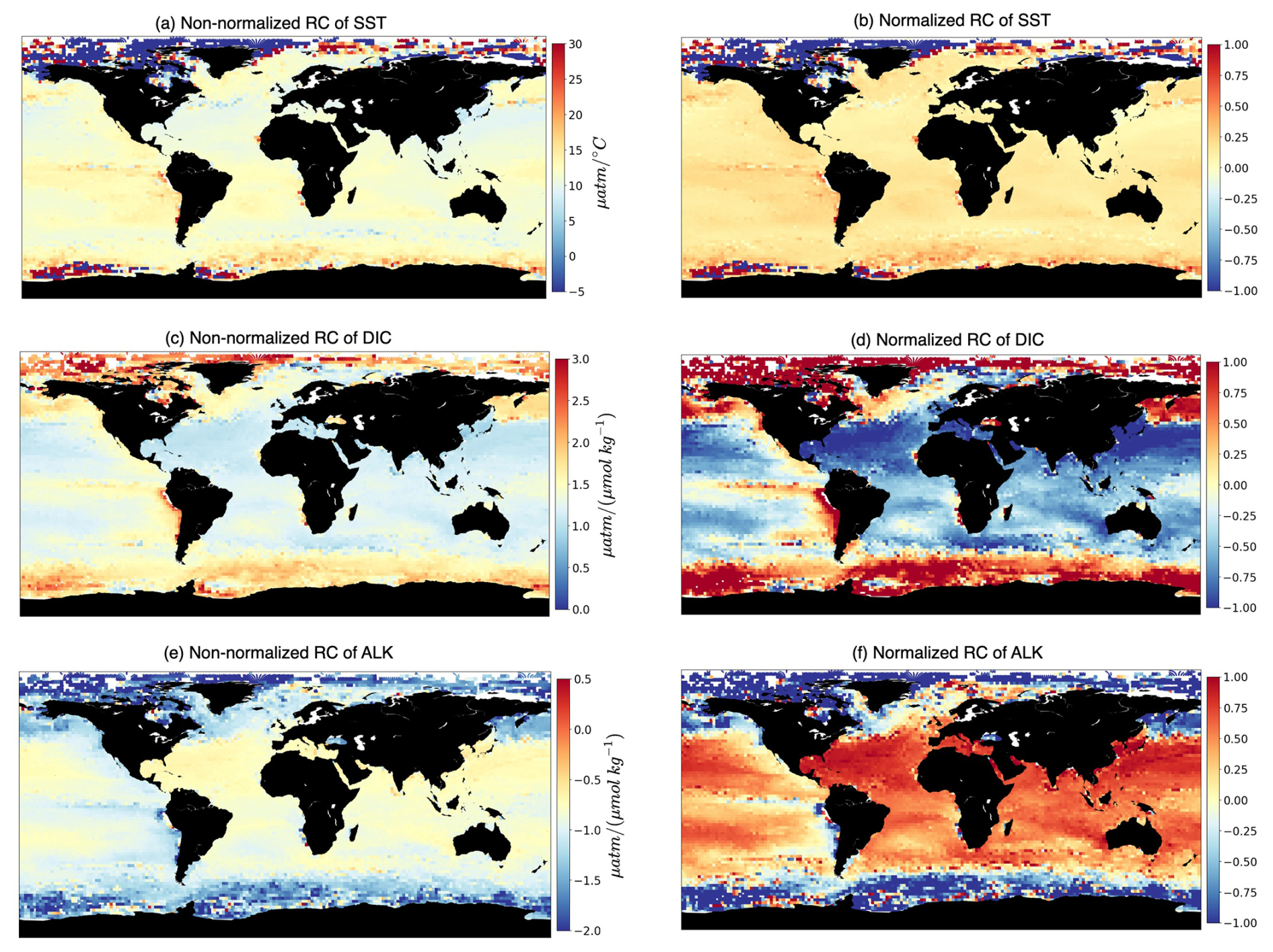
Figure 2 Spatial multivariate linear regression coefficients. The maps show non-normalized (a, c, e) and normalized (b, d, f) regression coefficients (RCs) computed over 2°×2° boxes of fCO₂ with respect to its three drivers, i.e., (a, b) SST, (c, d) surface DIC, and (e, f) surface ALK.

We have chosen MLR over univariate linear regression because MLR allows for considering multiple factors simultaneously and can capture more complex relationships between predictors and the dependent variable than univariate regression, which considers only one predictor at a time. The RCs from MLR can differ in magnitude and even in sign from regression slopes computed using univariate regression (compare Figs. 2 and A1). This is not surprising since MLR attempts to optimize the R² score by fitting a hyperplane among the target and three drivers. As a result, RCs computed through MLR can be negative, even though the univariate target–driver relationship is positive (e.g., compare the fCO₂–ALK multilinear relationship in Fig. 2c with the univariate relationship in Fig. A1g). Finally, we have opted for MLR as a baseline approach. Furthermore, MLRs deliver an understanding of what has been learned due to their linear nature, thus facilitating the interpretability of the target–driver relationships.

2.3 Detection of carbon biomes using adaptive agglomerative hierarchical clustering

The RCs from the MLR (Sect. 2.2) serve as the foundation to detect the carbon biomes. Carbon biomes are detected based on the linear target–driver relationships obtained over 2°×2° boxes. We employ an unsupervised machine learning approach, namely the agglomerative hierarchical clustering (HC) technique (Müllner, 2011), to construct a dendrogram based on the aggregation of the MLR coefficients (RC_SST, RC_ALK, RC_DIC). Before applying the HC technique, the RCs are first normalized (Fig. 2d–f) to have a mean of zero and a standard deviation of 1. Normalizing RCs ensures that all variables contribute equally to the agglomeration process, regardless of their original scales. We select a hierarchical clustering method for two main reasons: (1) it prevents the necessity for a predetermined number of clusters, thus circumventing subjective bias, and (2) it simplifies the visual exploration of the resulting dendrogram, thereby aiding in the interpretation of pertinent clusters (carbon biomes) and underlying data distributions. Besides, hierarchical clustering enables the extraction of clusters with varying degrees of granularity when the dendrogram is cut at different levels (Lin et al., 2022). As an input to our HC algorithm, we have chosen the RCs of January 2009. The specific choice of year and month does not affect the biome outcome, as the normalized RCs of SST, DIC, and ALK distributions stay steady over the years (see Appendix H).

The HC algorithm initiates by treating each normalized RC of individual 2°×2° boxes as a distinct cluster. Subsequently, pairs of singleton clusters are iteratively merged until all clusters combine into one prominent cluster, encompassing all locally linear regression models. In conjunction with Euclidean distance (the distance between two points in space in the feature space), Ward linkage is employed to construct the dendrogram. The Euclidean distance ed(p,q) between two data points (i.e., Euclidean distance between the RCs of two grid boxes) p and q is measured as shown in Eq. (2).

$$\begin{array}{}\text{(2)}& \begin{array}{rl}& \mathrm{ed}(p,q)=\\ & \sqrt{{\left(q_{{\mathrm{coef}}_{\mathrm{SST}}}-p_{{\mathrm{coef}}_{\mathrm{SST}}}\right)}^{\mathrm{2}}+{\left(q_{{\mathrm{coef}}_{\mathrm{DIC}}}-p_{{\mathrm{coef}}_{\mathrm{DIC}}}\right)}^{\mathrm{2}}+{\left(q_{{\mathrm{coef}}_{\mathrm{ALK}}}-p_{{\mathrm{coef}}_{\mathrm{ALK}}}\right)}^{\mathrm{2}}}\end{array}\end{array}$$

The Ward linkage is based on a method that combines data points to get compact clusters that minimize variance (in the ML literature, it is known as the Ward distance minimization algorithm; Müllner, 2011). It aims to lower the variance while combining two clusters, and the Euclidean distance (i.e., the straight-line distance between two points in space calculated using Pythagorean theorem) quantifies the distance between two clusters by measuring the increase in the sum of squares of individual clusters following their combination. The heights of the U-shaped links within the dendrogram signify this merging distance (i.e., the merging cost) in terms of the Euclidean distance. In other words, two branches that combine and build a cluster together on the vertical axis (in the ML literature, merging at a higher height) are more dissimilar (have a higher merging cost) than two branches merging at a lower height.

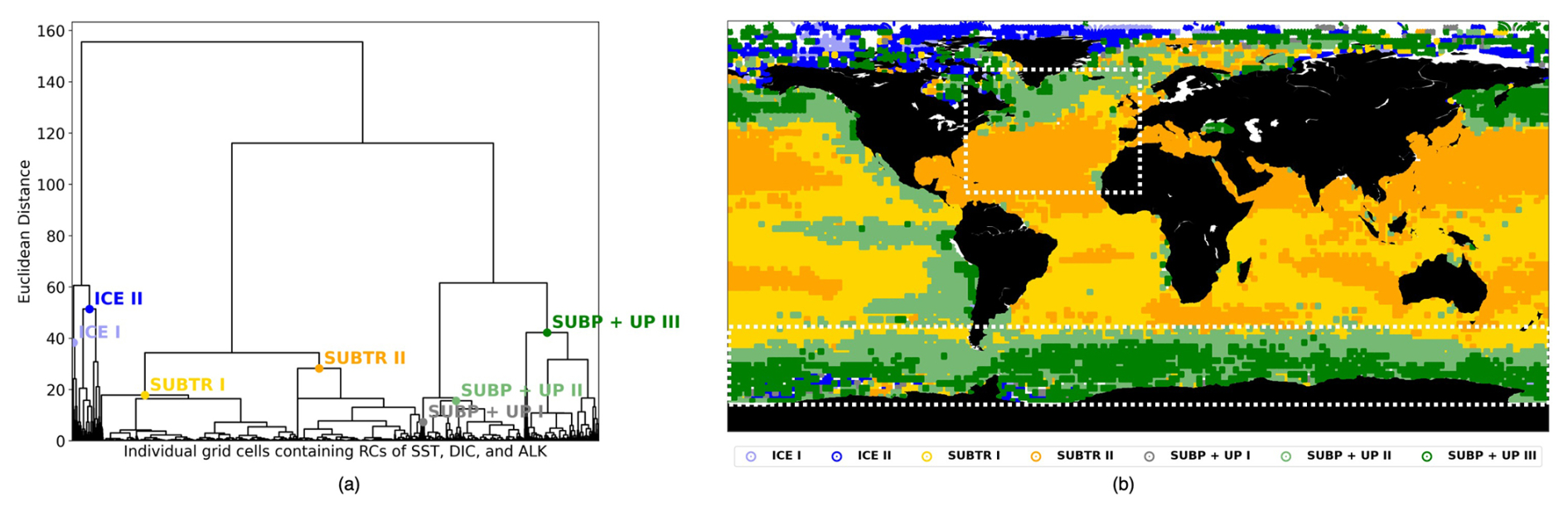
Figure 3 Carbon biomes in January 2009 detected through hierarchical clustering (HC). (a) Dendrogram resulting from the HC, with local cuts based on the distance–variance selection methodology. The text indicates the names of the detected seven clusters (i.e., the carbon biomes). (b) Geographical location of the detected clusters. The white boxes illustrate the basins – the North Atlantic between 75–0° W and 10–70° N and the Southern Ocean between 45–77° S – which will be analyzed in Sect. 3.2.

In a recent study (Mohanty et al., 2023a), we found that the conventional approach for identifying clusters within a dendrogram, entailing the selection of a specific distance value along the dendrogram's vertical axis, is not optimal for capturing the local statistical distributions, which vary substantially among branches. Because of unequal data distribution among the dendrogram branches, selecting a global cut at a lower distance would result in an excessive number of clusters on one branch, whereas picking a cut at a higher distance value would produce too few clusters on another branch (Fig. 3a). To overcome this limitation, Mohanty et al. (2023a) devised a novel adaptive approach to provide local cuts to the dendrogram. The method relies on the distance–variance selection technique and detects multiple local cuts on the dendrogram by considering both the compactness and similarity of the clusters. This algorithm operates based on two parameters, the change in distance (ΔDist) and the change in variance (ΔVar), that indicate the changes in distance and variance between different U-shaped links while traversing down the dendrogram from its root to its leaf nodes. This adaptive method serves the dual purpose of ensuring that the resultant clusters, representing carbon biomes, exhibit similarity and compactness, thus enhancing the robustness of cluster detection.

As we did not fix the number of provinces to be detected, we chose Bayesian information criterion (BIC) scores to select a meaningful partitioning (see evaluation in Appendix B). BIC scores are a statistical measure that augments the identification of an optimal number of clusters that effectively capture the underlying structure, balancing goodness of fit and model complexity. As detailed in Appendix B, we conducted 16 experiments with different parameter choices for ΔDist and ΔVar. Based on our evaluation, we opted for ΔDist=25.0 and ΔVar=0.1, as we can already distinguish distinct clusters with the lowest difference in the distance with the fixed difference in variance.

2.4 Tracking carbon uptake provinces using feed-forward neural networks

After having recognized the carbon biomes on the dendrogram, our intent now is to monitor their dynamics over time, revealing any evolving patterns within them. Since each biome is defined by the regression coefficients (RCs) of the drivers, obtaining localized RCs for subsequent months becomes mandatory. However, conducting adaptive clustering again in another month poses the challenge of connecting and matching two sets of identified biomes. Moreover, performing one-to-one matching based solely on RCs without location information is challenging. Hence, we shifted our focus to training neural networks to monitor and track carbon biomes over time. Based on the data from the initial month of the temporal sequence, the clustering process detects distinct carbon biomes. These clusters are identified and labeled, forming the foundation for subsequent tracking. The RCs of subsequent months are fed to the feed-forward neural networks (FNNs) as a classification problem to categorize them into distinct carbon uptake provinces.

We chose a feed-forward neural network for predicting the carbon biomes for two main reasons – nonlinearity detection and making the deep learning model scalable. (1) Nonlinearity detection: as the association between coefficients of SST, DIC, and ALK and the cluster labels is complex and cannot be defined by a linear relationship, FNNs can capture the underlying intricate patterns effectively. FNNs can learn elaborate interactions among input features(coefficients of SST, DIC, and ALK), which is crucial when predicting carbon biomes. For example, the impact of SST will vary from one spatial location to the other depending on the concentration of DIC or ALK, and a neural network is able to learn such relationships from the data. The FNNs' ability to model nonlinear connections is promising when dealing with multidimensional environmental variables. (2) Scalability during model construction: FNNs are versatile and allow flexibility in designing the model architecture, i.e., the number of layers, neurons per layer, and activation functions. FNNs can be scaled up by adding more layers or neurons to accommodate larger datasets and to learn more complex relationships between drivers and their targets. This adaptability enables the network to adapt to the sophistication of the data and biome labels, thus improving prediction accuracy.

Our tracking step involves training FNNs using the labeled carbon biomes obtained from the initial month as target labels. These neural networks are trained using this labeled dataset to learn the underlying patterns and relationships within the clusters. The inputs to the FNNs are the regression coefficients of SST, DIC, and ALK of January 2009 (see Appendix H). The aim is to impart the network with the ability to discern and predict the connection of data (regression coefficients of the drivers) to the identified clusters based on their respective characteristics. It focuses mainly on the features that define carbon biomes. Once trained, these neural networks are deployed to predict or assign cluster labels to the data points observed in the subsequent months of the temporal series. With the training process, the model learned to associate different RCs with different carbon regimes. Then, we use the same trained model to predict and track carbon provinces from January 1958 to December 2018.

For the tracking task, our FNN model comprised multiple dense layers with rectified linear unit (ReLU) (Agarap, 2018) activation functions interspersed with dropout layers for regularization. The model architecture consisted of an input layer followed by several hidden layers, each containing 64, 128, 256, 128, and 64 neurons. The choice of ReLU activation functions in the hidden layers facilitates the learning of nonlinear relationships within the data. Furthermore, L2 regularization with a regularization parameter of 0.01 was applied to the kernel weights of each dense layer to mitigate overfitting. The output layer, comprising seven neurons, utilized the softmax activation function (Goodfellow et al., 2016) to deliver a probability distribution over the seven classes of carbon biomes. The model was trained using the ADAM (Adaptive Moment Estimation) (Kingma and Ba, 2017) optimizer with a learning rate of 0.001 optimized for categorical cross-entropy loss. Additionally, performance metrics such as accuracy, precision, and recall were monitored during training to assess the model's predictive capabilities. The training process was conducted over 50 epochs with a batch size of 32, and the model's performance was evaluated on a validation dataset. Overall, the implemented FNN architecture with appropriate regularization and optimization techniques aimed to effectively capture the underlying patterns in the data and achieve robust classification performance. To prevent overfitting, early stopping with patience of five epochs was employed as a regularization technique. This led to finishing our training within 30 epochs.

We relied on metrics such as accuracy, precision, and recall to assess the performance of our FNN model in the context of multiclass prediction tasks. Accuracy measures the correctness of the model's predictions across all biome labels. It is calculated as the ratio of the number of correctly predicted cases to the total number of cases in the dataset. For a particular cluster label, precision measures correctly predicted instances over all the instances that are predicted as that specific class or biome label. Furthermore, for a respective cluster label, recall is the proportion of correctly classified instances over all the instances of that specific class or biome label. The different parts of the FNN are explained in Appendix D.

It is worth mentioning that an alternative method was tested in the past for tracking the carbon biomes (Mohanty et al., 2023a), where we experimented with whether the carbon biomes could be tracked only based on the changes in the feature–driver relationships over time. Specifically, we ran the HC algorithm for every month of each year. Then, we calculated the Frobenius norm, a distance metric, between the normalized RCs of each cluster between one step and the next. We subsequently matched the clusters exhibiting the lowest Frobenius distance. However, this approach was not optimal since the cluster numbers returned by our adaptive HC were not fixed, and the Frobenius norm failed to match all clusters over time. Through our current study, we trained a neural network to learn the associations between labels and the underlying regression coefficients (RCs). This allowed us to predict the locations of the same labels over time in an effective way. As shown in Fig. H1, the normalized RCs within each biome are (with the exception of the strongly variable ICE biomes) substantially stable over all months and years.

3 Results

3.1 Detection of carbon biomes

The relationship between fCO₂ and its three drivers (hereafter called RC_SST, RC_DIC, RC_ALK) exhibits large spatial variations (Fig. 2), indicative of different dynamics acting over different regions of the global ocean. We find an expected positive relationship of fCO₂ with respect to SST over large swaths of the global ocean (Fig. 2a) since higher SST reduces the seawater CO₂ solubility and, thus, enhances its fugacity at the ocean surface. Over most of the global ocean RC_SST is typically included between 10 and 16 µatm °C⁻¹. When pCO₂ is affected only by temperature, Takahashi et al. (1993) determined a relative variation in pCO₂ of 0.0423 °C⁻¹, equivalent to 16.9 µatm °C⁻¹ for a pCO₂ value of 400 µatm. The deviation of our simulated RC_SST from this expected value indicates the influence of non-thermal processes on fCO₂. Also, we are considering RCs from multilinear regressions which, as mentioned in Sect. 2.2, may differ from the univariate perspective. At polar latitudes, RC_SST values are much higher, are mostly negative, and are characterized by higher spatial variability. In this respect, the following points should be considered: (i) SST in polar regions deviates only slightly from the freezing temperature (Fig. A1), which leads to high RC_SST even in the presence of moderate variations in fCO₂. (ii) The rather counterintuitive negative RC_SST values can be understood by considering that when an increase in surface temperature melts sea ice, the ensuing air–sea CO₂ exchanges and phytoplankton growth lead to a reduction of fCO₂. (iii) Leads and fractures in sea ice may generate a strong spatial variability in fCO₂ due to the array of processes (air–sea CO₂ exchanges, biological productivity) which are set in motion when a previously sea-ice-covered region is exposed to the atmosphere. RC_DIC is positive basically everywhere, indicating an expected positive dependence of fCO₂ on DIC. RC_ALK is instead mostly negative since increases in ALK have a buffering effect on fCO₂. RC_DIC and RC_ALK therefore tend to have opposite and specular effects on fCO₂ (Fig. 4c).

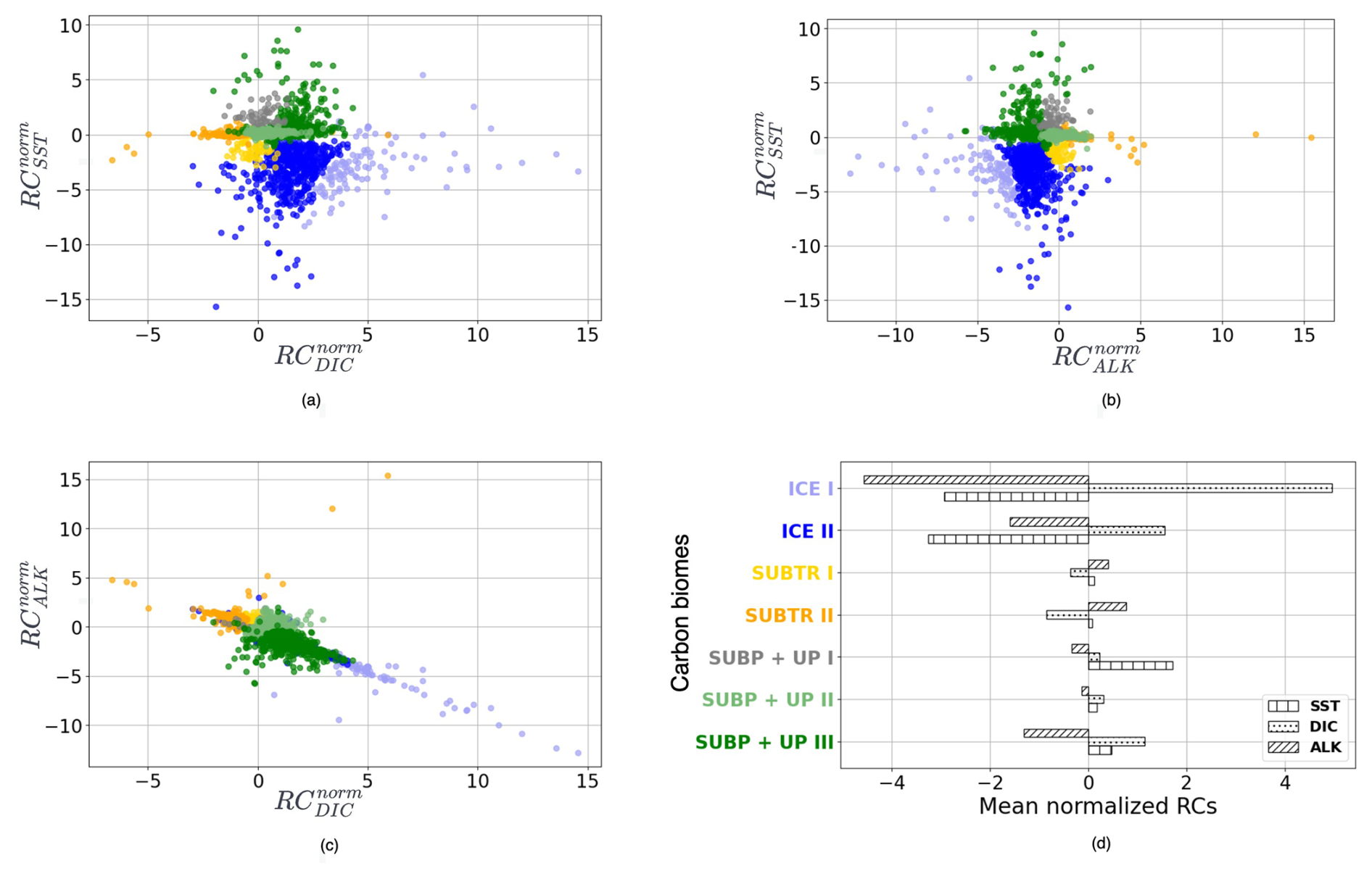
Figure 4 Distribution of normalized regression coefficients (RC^norm) in the carbon biomes detected for January 2009. (a) RC${}_{\mathrm{SST}}^{\mathrm{norm}}$ against  ${}_{\mathrm{DIC}}^{\mathrm{norm}}$, (b) RC${}_{\mathrm{SST}}^{\mathrm{norm}}$ against RC${}_{\mathrm{ALK}}^{\mathrm{norm}}$, (c) RC${}_{\mathrm{ALK}}^{\mathrm{norm}}$ against RC${}_{\mathrm{DIC}}^{\mathrm{norm}}$. (d) RC${}_{\mathrm{SST}}^{\mathrm{norm}}$, RC${}_{\mathrm{DIC}}^{\mathrm{norm}}$, and RC${}_{\mathrm{ALK}}^{\mathrm{norm}}$ averaged over the carbon biomes. Colors indicate the detected carbon biomes: ICE biomes in blue shading, SUBP+UP biomes in green shading, and SUBTR biomes in orange shading. SUBP+UP I was not tracked (see main text) and is therefore shown in gray.

The RCs resulting from the MLR have been normalized before being fed to the hierarchical clustering (HC) algorithm (Sect. 2.3) so that, over the globe, RCs for each driver have a mean of zero and a standard deviation of 1 (Fig. 2, right column). The normalized RCs (hereafter RC^norm) can thus be understood as anomalies with respect to the global mean. As an example, negative values of RC${}_{\mathrm{DIC}}^{\mathrm{norm}}$ over the subtropical gyres indicate a dependence of fCO₂ on DIC that is lower than the global average. The HC algorithm run on RC^norm values of January 2009 produces the dendrogram shown in Fig. 3a. As explained in Sect. 2.3, the resulting clusters depend on the choice of where to cut the dendrogram. Instead of selecting a fixed height for the dendrogram cut, we used the distance–variance selection methodology (Mohanty et al., 2023a) to define local cuts based on the underlying data distribution. This procedure yields a total of seven carbon biomes, each possessing analogous characteristics in terms of target–driver relationships (Fig. 4a–c). The dendrogram detects three main branches, exhibiting distinct combinations of RC^norm values (Fig. 4d) and specific geographical locations (Fig. 3b).

The leftmost branch on the dendrogram detaches itself from the other branches at an elevated height, indicating that it is very dissimilar from the other two branches. This branch is located at polar latitudes in all months, especially in the Arctic (blue in Figs. 3b, 5a, b and C1), and is hereafter called the ICE branch. The ICE branch distinguishes itself by having strongly negative RC${}_{\mathrm{SST}}^{\mathrm{norm}}$ and RC${}_{\mathrm{ALK}}^{\mathrm{norm}}$ and strongly positive RC${}_{\mathrm{DIC}}^{\mathrm{norm}}$ (Fig. 4). The ICE branch is thus characterized by large spatial gradients in fCO₂ and its drivers, negative dependence from SST, and a strong positive dependence on DIC. Our analysis thus suggests that the ICE branch is mostly driven by non-thermal processes but is characterized by a distinctive dependence of fCO₂ on SST due to the interaction with sea ice (as explained above). Based on our parameter choice, two ICE sub-branches are identified as biomes (ICE I and ICE II). The two ICE biomes are characterized by different magnitudes (but the same sign) of the RC^norm values. Specifically, ICE I corresponds to fewer boxes and is characterized by the most extreme values of the RC^norm, whereas ICE II covers larger parts of the polar ocean and has somewhat lower magnitudes of RC^norm values.

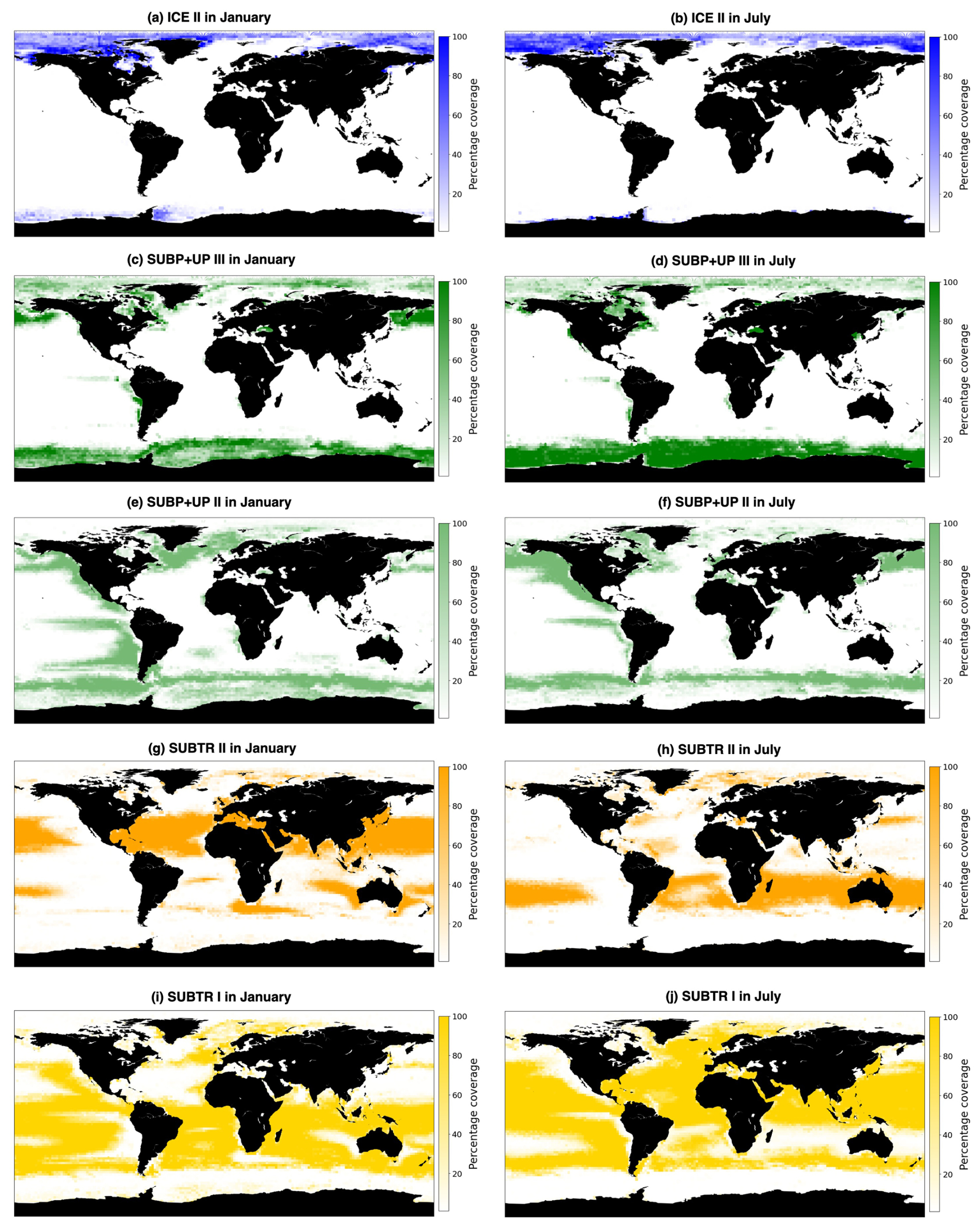
Figure 5 Percentage coverage of carbon biomes over the years 1958 to 2018, where a value of 100 % indicates that the biome is present in each simulation year in the 2×2 box and a value of 0 % that it is never present in the 2×2 box. Shown are the five main carbon biomes: (a, b) ICE II, (c, d) SUBP+UP III, (e, f) SUBP+UP II, (g, h) SUBTR II, and (i, j) SUBTR I in January (a, c, e, g, i) and July (b, d, f, h, j).

The rightmost branch on the dendrogram is geographically located at subpolar latitudes as well as in upwelling regions, i.e., equatorial Pacific and coastal upwelling areas (green in Figs. 3b, 5c–f and C1). This branch, which we call SUBP+UP, distinguishes itself from the other two branches by having positive values of RC${}_{\mathrm{SST}}^{\mathrm{norm}}$ and RC${}_{\mathrm{DIC}}^{\mathrm{norm}}$ and negative values of RC${}_{\mathrm{ALK}}^{\mathrm{norm}}$ (Fig. 4d). RC${}_{\mathrm{DIC}}^{\mathrm{norm}}$ always has a larger magnitude than RC_SST, suggesting increased importance of non-thermal processes in driving fCO₂ variability in those regions. The selected parameter settings detect three SUBP+UP biomes (SUBP+UP I, SUBP+UP II, SUBP+UP III), each characterized by different flavors of the RC^norm combinations. SUBP+UP III is characterized by the highest RC${}_{\mathrm{DIC}}^{\mathrm{norm}}$ values of this branch, suggestive of a stronger dependence of fCO₂ on non-thermal processes, and is predominantly located in high-latitude subpolar areas (Fig. 5c and d). SUBP+UP II is characterized by small values of all three RC^norm values (i.e., they are closer to the global mean) and often marks the transition towards midlatitude and subtropical regimes (Fig. 5e and f). SUBP+UP I has a strongly positive RC${}_{\mathrm{SST}}^{\mathrm{norm}}$ and is found at the edge with the ICE branch (Fig. 3b). However, since it contained only 0.55 % of the total sample size, it was discarded from the tracking process (see Sect. 3.2).

The middle branch in the dendrogram is geographically located in the tropics, in the subtropical gyres, and in large parts of the North Atlantic (orange in Figs. 3b, 5g–j and C1). This branch, which we call SUBTR, distinguishes itself from the other two branches by having positive values of RC${}_{\mathrm{SST}}^{\mathrm{norm}}$ and RC${}_{\mathrm{ALK}}^{\mathrm{norm}}$ and negative values of RC${}_{\mathrm{DIC}}^{\mathrm{norm}}$ (Fig. 4d). Negative (positive) values of RC${}_{\mathrm{DIC}}^{\mathrm{norm}}$ (RC${}_{\mathrm{ALK}}^{\mathrm{norm}}$) are indicative of regions where the dependence of fCO₂ on DIC and ALK is lower than the global average. This combination of RC values suggests the enhanced importance of thermal processes in driving fCO₂ variability in the SUBTR branch. The HC algorithm detects two SUBTR biomes (SUBTR I and SUBTR II), characterized by different flavors of RC^norm combinations. In SUBTR II, RC${}_{\mathrm{DIC}}^{\mathrm{norm}}$ is particularly low and is located in the central parts of the subtropical gyres (Fig. 5g and h). SUBTR II is, therefore, identified as the biome most strongly driven by thermal processes. SUBTR I is instead characterized by more moderate values of RC^norm and is found over large swaths of the global ocean, including subtropical, middle, and even subpolar latitudes (Fig. 5i and j).

Finally, it should be noted that the RC^norm values are more compact over the SUBTR biomes and SUBP+UP II biomes than over the remaining biomes. This can be visualized in Fig. 4a–c, where a large variance around the mean is found for the ICE and SUBP+UP I biomes. This different statistical distribution of the data within the different dendrogram branches is one of the reasons why, for this dataset, local cuts to the dendrogram work better than a fixed global cut.

3.2 Tracking of carbon biomes

Temporal tracking of carbon biomes was performed using a forward-feed neural network (FNN) model. The inputs to the FNN model are the RC^norm values obtained through MLR, and the target labels are the seven carbon biomes detected on the dendrogram (Fig. 1). As explained in Sect. 2.4 and further discussed in Sect. 4, we selected January 2009 as the month for which to run the HC and produce the biome labels and temporally predicted all other months during the 1958–2018 period using FNN. 80 % of the RC^norm values were used for training and validation, and the remaining 20 % were used to test the learned model. During training, the validation accuracy reached 94.81 %, precision was 95.22 %, and recall stood at 94.06 %. The good results from our FNN model on the training data were also reflected in the test data, where we obtained a test accuracy of 94.83 %, precision of 95.39 %, and recall of 94.5 %. We have chosen the biomes predicted by the FNN with the highest probability. More information on FNN evaluation can be found in Appendix D, including the confusion matrix on the test set, highlighting the abovementioned values of test accuracy, precision, and recall (Fig. D1e). The biome SUBP+UP I contained only 0.55 % of the total sample size and was excluded by the FNN model while learning the relationships between the biome label and the RCs.

The tracking of carbon biomes allows us to address the following questions: (Q1) does the geographical location of the biomes vary significantly from year to year? (Q2) Are there seasonal fluctuations of the biome coverage in the course of a year? (Q3) Are there year-to-year changes and long-term trends in the biome coverage in response to climate variability and change? It should be stressed that both the detection and the tracking are solely based on the RC${}_{\mathrm{SST}}^{\mathrm{norm}}$, RC${}_{\mathrm{DIC}}^{\mathrm{norm}}$, and RC${}_{\mathrm{ALK}}^{\mathrm{norm}}$ values, without any prior knowledge of the geographical locations of the biomes. The temporal tracking is, therefore, a purely location-agnostic process that depends only on the carbon dynamics specific to that region.

Figure 5 shows the percentage coverage of the five main biomes (SUBTR I, SUBTR II, SUBP+UP II, SUBP+UP III, ICE III) computed over the 1958-2018 period, distinguishing between January and July. All biomes are characterized by core regions where the coverage reaches 100 %, peripheral regions where the biome is found only in some years, and external regions where the biome is never detected. From Figs. 5 and 6c–f, we see that the biome coverage is overall consistent from year to year, indicating that the trained FNN is able to consistently predict regions with similar RC patterns over time. Only a couple of years were found to be inconsistent with the overall pattern. The occasional abrupt shifts in biome coverage (e.g., January 1969 and March 1958 in the North Atlantic and September 1969 in the Southern Ocean) are to be considered climate-driven transient features.

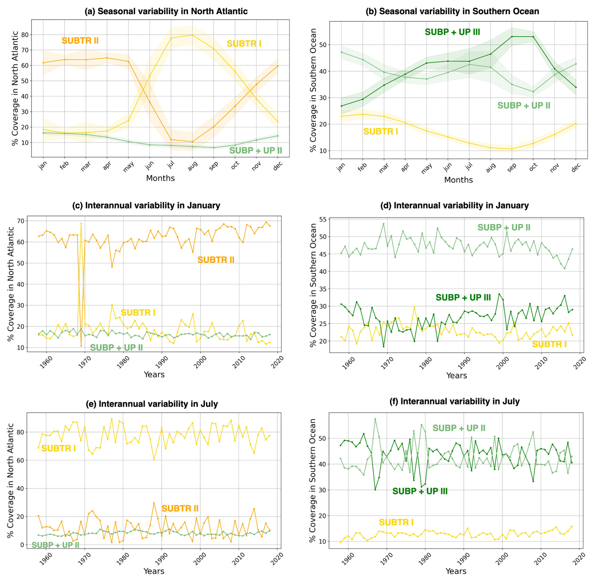
Figure 6 Seasonal and interannual variations of carbon biome coverage. Shown is the percentage coverage of the three main biomes over the North Atlantic (a, c, e) and Southern Ocean (b, d, f). The limits of the basins are shown in Fig. 3b. The percentage coverage is computed as the weighted area average of the carbon biome divided by the total area of the basin so that a value of 100 % would be achieved when the biome covers the whole basin. (a, b) Mean seasonal cycle of the carbon biome coverage, with shading indicating the standard deviation across the 61 simulation years. (c–f) Weighted area average of the percentage coverage of carbon biomes over 1958–2018 in the months of (c, d) January and (e, f) July. The North Atlantic basin lies between 75–0° W and 10–70° N, and the Southern Ocean is between 45–77° S.

Distinctive features characterize the different biomes in terms of seasonality. SUBTR II (Fig. 5g and h), the most thermally driven biome, seasonally dominates in the winter months in the subtropical gyres (i.e., in the Northern Hemisphere in January and in the Southern Hemisphere in July). This is possibly related to the fact that in winter when there is little biological productivity, fCO₂ is mostly driven by SST. SUBTR I (Fig. 5i and j), covering large swaths of the global ocean, has a tendency for higher coverage in the summer months. This is potentially because SUBTR I has a less pronounced thermal control than SUBTR II and, therefore, dominates in locations and months for which non-thermal processes also play some role. SUBP+UP III has its greatest extent in the winter months of the subpolar and high latitudes when strong non-thermal controls (e.g., convection and upwelling) drive fCO₂. In the summer months, SUBP+UP II, with its somewhat more nuanced non-thermal control, occupies subpolar areas occupied by SUBP+UP III in winter. An exception is the North Atlantic, as will described later on. ICE II is found almost exclusively in the Arctic Ocean, with little seasonal variation.

The biome coverage and underlying environmental properties are further explored for two basins of climatic relevance (contours in Fig. 3b): (1) the North Atlantic between 75–0° W and 10–70° N and (2) the Southern Ocean between 45 and 77° S. Figure 6a and b show the mean seasonal evolution of the percentage coverage of the three main biomes for each basin, with the standard deviation computed over the 61 simulation years shown as shading. 100 % coverage for a biome thus would indicate that the biome covers the whole basin, whereas 0 % coverage indicates that the biome never occurs in the basin. To gain a better perspective of the environmental conditions affecting each biome, we further analyzed the mean seasonal cycle of SST, sea surface salinity (SSS), and mixed layer depth (MLD) over each of the three main biomes detected in the two basins (Fig. 7). In analyzing these seasonal cycles of environmental parameters, it should be remembered that the area on which the averages are computed changes with time, which can complicate the interpretation. However, we believe this analysis is still useful as it allows us to better characterize the biomes in terms of environmental properties.

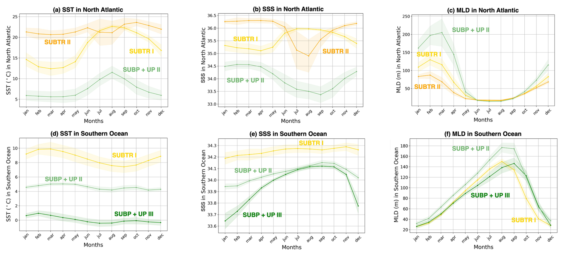
Figure 7 Seasonality of environmental parameters over biomes in the North Atlantic and Southern Ocean. Mean seasonal cycle over 1958–2018 of (a, d) SST, (b, e) sea surface salinity (SSS), and (c, f) mixed layer depth (MLD), averaged within the three main carbon biomes in the North Atlantic (a–c) and Southern Ocean (d–f). The limits of the basins are shown in Fig. 3b. Shading indicates the standard deviation over the 61 simulation years. The North Atlantic basin lies between 75–0° W and 10–70° N, and the Southern Ocean is between 45–77° S.

The North Atlantic (NATL) exhibits a sharp divide between the subtropical and subpolar gyres, separated by the North Atlantic Current (Fig. 5). SUBTR I and SUBTR II seasonally compete, with SUBTR I dominating in summer (around 80 % of the whole NATL) and SUBTR II in winter (around 60 % of the whole NATL) (Fig. 6a). SUBTR II shows overall the highest SST and SSS and the lowest winter MLD (Fig. 7a–c), consistent with the strongly stratified subtropical gyre conditions. A dip in SST and SSS in July–August, with elevated uncertainty levels, is connected to the very low coverage of SUBTR II in these months (Fig. 5h), an aspect which amplifies the importance of limited coastal and high-latitude regions. SUBP+UP II, the third most represented biome in the NATL, gains its highest coverage in winter (around 20 % of the whole NATL). SUBP+UP II is mostly found in the subpolar NATL (Fig. 5e and f), where it seasonally competes with SUBTR I, which is instead most present in summer. Interestingly, in the eastern parts of the subpolar North Atlantic, SUBTR I dominates in both winter and summer (Fig. 5i and j), possibly because of the influence of the North Atlantic Current bringing subtropical waters to those areas. In other words, from a carbon perspective, the eastern subpolar NATL is more similar to midlatitude and subtropical domains than the western subpolar NATL. As expected, SUBP+UP II has lower SST (with a peak and summer) and the deepest winter MLD with respect to the SUBTR biomes (Fig. 7a–c). The dip in SSS in the summer months is likely related to the fact that in summer SUBP+UP II mostly occupies sea ice melting regions (Fig. 5f).

The Southern Ocean (SO) exhibits a seasonal competition of SUBTR I, SUBP+UP II, and SUBP+UP III (Fig. 6b). SUBP+UP III is the coldest biome (Fig. 7d), and it occupies the subpolar regions dominated by wind-driven upwelling and moderately deep mixed layers (Fig. 7f). It is most extended in winter when it covers more than 50 % of the whole SO. The enhanced SSS in the winter season (Fig. 7e) is consistent with the increased wind-driven upwelling of relatively salty Circumpolar Deep Water in the winter months. In the summer months, SUBP+UP III recedes, and SUBP+UP II gains more relevance (Fig. 6b). SUBP+UP II is overall warmer than SUBP+UP III and is found in midlatitude regions characterized by deep winter MLD (Sallée et al., 2021). In all months, SUBP+UP II typically follows the path of the Antarctic Circumpolar Current as well as water mass formation areas to the north of it (Fig. 5e and f). SUBTR I, with its higher SST and SSS, is a more thermally driven biome with the highest coverage in the summer months (Fig. 6b).

When performing the carbon biome tracking over the whole 1958–2018 period, we find that some biomes have expanded, whereas some have shrunk. In the NATL, SUBTR I and SUBTR II, which compete on seasonal timescales, show anticorrelated interannual variability over the 1958–2018 period. In winter, SUBTR I and SUBTR II also show diverging trends since the 1970s, with SUBTR II expanding by about 10 % at the expense of SUBTR I. This might be related to a concomitant increase in SST over the North Atlantic subtropical gyre (Bulgin et al., 2020), which might have enhanced the thermal control of SST on fCO₂. In the Southern Ocean, SUBP+UP II and SUBP+UP III show competing variabilities on interannual timescales and – since the late 1960s – an overall 10 % increase in SUBP+UP III in summer at the expense of SUBP+UP II. This might be related to the concomitant increase in Southern Hemisphere westerly winds (Swart et al., 2015), which has created more favorable conditions for DIC upwelling and therefore enhanced the non-thermal control on fCO₂ (Gruber et al., 2023).

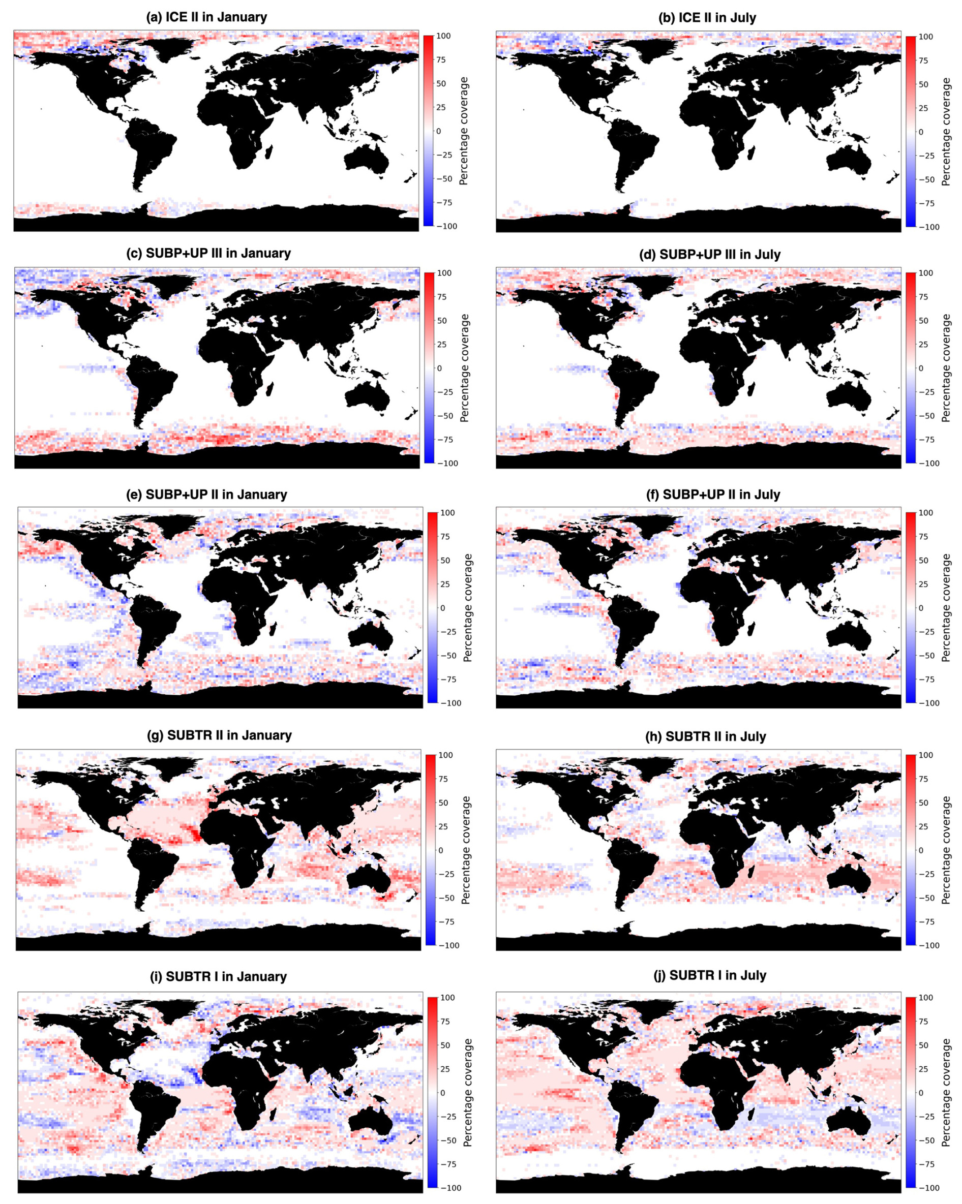
Figure 8 Change in the percentage coverage of carbon biomes between 1970–1979 and 2009–2018. Shown are the five main carbon biomes: (a, b) ICE II, (c, d) SUBP+UP III, (e, f) SUBP+UP II, (g, h) SUBTR II, and (i, j) SUBTR I in January (a, c, e, g, i) and July (b, d, f, h, j). As an example, a value of +100 % indicates that over a 2° box, a particular biome was present for each of the 10 years from 2009–2018 and never present in any of the 10 years between 1970–1979. Conversely, a value of −100 % indicates that the biome was always present from 1970–1979 and never in 2009–2018. A value of 0 % indicates that the biome was equally present between the two decades.

Additionally, to better understand and visualize the trends in biome coverage over the global ocean, we have computed (i) the coverage change for five biomes between 1970–1979 and 2009–2018, as shown in Fig. 8; (ii) the trends in biome coverage between 1970 and 2018 over the North Atlantic Ocean and Southern Ocean for all months (not only January and July), as presented in Table E1; and (iii) the changes in SST between 1970–1979 and 2009–2018 in both the model and the observation-based dataset EN4.2.2 (Good et al., 2013), shown in Fig. F1, to interpret the trends in the context of the changing climate. Table E1 shows that, in the North Atlantic, the percentage coverages of the SUBTR I and SUBTR II biomes are negatively correlated and show opposing linear trends between 1970–2018 for each month of the year. While the correlations are always statistically significant (p<0.04), the linear trends are statistically significant only between January and May. Over these months, SUBTR II (the most thermally driven biome) expanded at a rate of ∼1 %–2 % per decade, while the SUBTR I biome contracted at a similar rate. Locally, the trends in biome coverage may reach even higher values; i.e., the changes may exceed 50 % between the decade 1970–1979 and the decade 2009–2018, as shown in Fig. 8. Figure 8 also shows that SUBTR II expanded in all basins in the winter hemisphere (January in the Northern Hemisphere, July in the Southern Hemisphere) at the expense of SUBTR I, which instead expanded in the summer hemisphere and the tropics. The expansion of the SUBTR II biome could be related to a concomitant increase in SST over the North Atlantic and subtropical gyres (Fig. F1), in agreement with the observational dataset EN4.2.2 (Good et al., 2013). This might have enhanced the thermal control of SST on fCO₂, thereby favoring the thermally driven SUBTR II biome. We can further speculate that the expansion of SUBTR II is particularly strong in winter, which may be related to the low phytoplankton carbon uptake in these months, a characteristic that enhances the thermally driven character of the biome. In the Southern Ocean, the percentage coverages of the SUBP+UP II and SUBP+UP III biomes are also negatively correlated on interannual timescales and mostly show opposing linear trends between 1970–2018 (Table E1). The statistically significant trends are found here in the summer months (December–March), with an expansion of the non-thermally driven SUBP+UP III biome of 0.5 %–1 % and a contraction of the SUBP+UP II biome. Again, locally the trends in biome coverage may reach values exceeding 50 % between the decade 1970–1979 and the decade 2009–2018. The expansion of the non-thermally driven SUBP+UP III biome might be related to the concomitant increase in Southern Hemisphere westerly winds (Swart et al., 2015), which has created more favorable conditions for DIC upwelling and therefore enhanced the non-thermal control on fCO₂ (Gruber et al., 2023). The increased upwelling caused a negative trend in SST (Fig. 4), which in the model is particularly strong in the austral summer months and much less pronounced in the austral winter months. This might explain why the expansion of SUBP+UP III was stronger in the austral summer months. However, since this winter–summer asymmetry is not visible in the observation-based EN4.2.2 dataset, it remains uncertain whether the model might underestimate the SUBP+UP III expansion in winter.

4 Discussion and conclusions

In the framework of a rapidly evolving climate and ocean carbon cycle, the aim of this study was to develop a machine learning tool to detect ocean carbon biomes and track them under seasonally and interannually varying environmental conditions. We defined carbon biomes as regions having consistent relations between surface CO₂ fugacity (fCO₂) and its main drivers (temperature, dissolved inorganic carbon, and alkalinity). With a combination of localized multilinear regression (MLR) models, agglomerative hierarchical clustering (HC), and a forward-feed neural network, we were able to successfully detect and track ocean carbon biomes both seasonally and over the 1958–2018 period. The key features and novelties in our study are (i) employing target–driver relationships as an input to the HC algorithm, instead of directly feeding in the environmental parameters to the clustering method; (ii) using a distribution-aware clustering method to group these relationships, ensuring that each group is compact and cohesive, with similar internal relationships; and (iii) building a tool to track the evolution of the detected clusters or carbon regimes over time. This methodology enabled us to detect well-defined carbon biomes (representative of subtropical, upwelling, subpolar, and sea-ice-covered regimes) whose geographical location and spatial extent responded meaningfully to seasonal and interannually varying environmental conditions. It is to be stressed that the detection and tracking of the carbon biomes were done entirely without providing any information about the geographical location of the biomes. The fact that the detection uncovered biomes with meaningful geographical characteristics is purely the result of the different ways in which the fCO₂ reacts to its drivers, which in turn is intimately intertwined with the underlying ocean dynamics.

There are a number of considerations that need to be made regarding our methodology and some aspects where we see room for improvement in future studies. For example, analyzing spatial target–driver relationships via methods focusing on polynomial functions with degree ≥ 2 and different neural network architectures could also be implemented. In order to construct labels needed to train the FNN, we needed to select a specific month and year (in this case, we selected January 2009). The question arises as to whether our results are sensitive to the choice of this selection. The regression coefficients (RCs) computed with MLR show a smooth transition from one month to another and are relatively invariant from one year to the next. Building upon this stability, we found that the carbon biomes detected for other random years are comparable to that based on the January 2009 baseline (not shown). However, we acknowledge that the month and year selection introduces a subjectivity that would be preferable to avoid. The hypothesis that the selection of different months and years may lead to different biome segmentations cannot be excluded, and we suggest that future work should investigate the volatility or stability of the chosen reference. Another option would have been to perform clustering on a monthly basis to detect the carbon biomes. However, this option comes with additional caveats. Firstly, employing HC with Ward linkage over an extensive spatial domain enclosing more than 10 000 grid boxes is intrinsically time-intensive. Secondly, the absence of an established technique to successfully match clusters between successive months beyond visual inspection is a big challenge. Given the broad temporal scope of our analysis traversing 732 months (61 years × 12 months), manual tracking via visual analysis would have been impractical and subjective. Therefore, we adopted a practical strategy where we labeled the seven detected clusters for one specific year and month and employed a neural network with predictive capacities to learn the intricate associations between the RCs and the assigned cluster labels. With the deep learning model successfully learning the subtle relationships between these variables, it can predict cluster labels based on input regression coefficients and corresponding probabilities. Subsequently, the carbon biomes predicted by the FNN with the highest probability are selected as the most probable clusters. Our study does not provide the exact locations of static biomes, but rather – due to the temporally varying nature of the ocean – a probability that a specific biome will be found in a particular place (Fig. 5). We acknowledge that it would be practical for model evaluation or intercomparison studies to define a set of static biomes over which different model diagnostics can be averaged (as done in, e.g., DeVries et al., 2023). However, the usage of static biomes comes with disadvantages owing to time-varying and model-specific locations of ocean fronts (Fay and McKinley, 2014). We suggest that future research could use the detection and tracking tool proposed here across different data classes to test the spatial homogeneity of the carbon biomes as well as to better understand the specific dynamics of each model.

Another aspect to consider regards the selection of feed-forward neural networks (FNNs), which come with several challenges that can hinder their effectiveness in certain applications. One primary concern is the complexity of FNN architectures, which may lead to overfitting and difficulty in interpretation due to the large number of parameters involved. Further, FNNs are often criticized for their black-box nature (Irrgang et al., 2021), as they lack clarity in the decision-making approach, making it demanding to comprehend how inputs are connected to outputs. While convolutional neural networks (CNNs) (LeCun et al., 2015) and long short-term memory (LSTM) (Hochreiter and Schmidhuber, 1997) networks are powerful alternatives to FNNs in certain contexts, they may not be well-suited for all tasks. CNNs are outstanding at pulling spatial features from data such as images, audio, and videos (Goodfellow et al., 2016), and LSTM networks are adept at apprehending temporal dependencies in sequential data. However, these methods may not have been suitable for our study. CNNs and LSTMs would have required not just one (as we utilized in our FNN model) but rather hundreds of annotated maps of global oceans depicting ocean biomes. Considering that we are operating with $\mathrm{61}\times \mathrm{12}=\mathrm{732}$ maps of RCs, either clustering or manually labeling half of them with respective biomes would have been required to train these models, while the remaining maps would have been utilized for biome tracking. Consequently, both clustering and manually determining the same biomes across multiple months would have been particularly time-consuming, compounded by the additional training time needed for these models. Essentially, we would have needed to specify the presence and locations of carbon biomes across multiple months even before initiating the tracking process. Additionally, we focused on optimizing the NN architecture's accuracy and precision with different hyperparameters. Experimenting with different nonlinear functions, individual weights, and biases for every layer of NN could be incredibly time-consuming. The opaque nature of neural networks makes precisely interpreting what each neuron has learned harder. This is especially true for deep networks with many layers. As a future study, interpretability techniques like layer-wise relevance propagation (LRP) (Binder et al., 2016), Shapely values (Hart, 1989), and LIME (Ribeiro et al., 2016) could be applied to understand essential features and how neurons or layers contribute to the model’s prediction capabilities.

The carbon biomes found in this study are geographically analogous to those found in past classification studies that focused on the ocean carbon cycle (Jones and Ito, 2019; Landschützer et al., 2016). Even though based on different classification methods and input parameters, the biomes found in these past studies resemble those found here. It can, therefore, be concluded that different carbon properties share a similar dependence on the underlying dynamical context (e.g., oligotrophic subtropical gyres vs. productive upwelling regions), which in our case translates into distinct spatial target–driver relationships between fCO₂ and its drivers. Also, similarly to Jones and Ito (2019) and Couespel et al. (2024), we find that the same biome can occur in distinct geographical locations. This can be seen for, e.g., the SUBP+UP biomes, which are found in both tropical and subpolar upwelling areas. The classification used here thus differs from that proposed by Fay and McKinley (2014), which involves splitting the ocean into four major ocean basins (Atlantic, Pacific, Indian, and Southern Ocean), followed by the application of criteria based on specific variable ranges (such as SST, MLD, chlorophyll concentration, and sea ice). The biomes found by Fay and McKinley (2014), which are widely used to evaluate and compare ocean carbon cycle models (DeVries et al., 2023), thus have a clear geographical separation, which instead somewhat breaks down in the clustering method used here. This result suggests that geographically separated regions can be more closely connected regarding ocean carbon dynamics than their geographical location would suggest.

In this investigation, we find three main dynamical branches (sea-ice-covered, subpolar + upwelling, and tropical + subtropical), each characterized by different combinations of spatial target–driver relationships and underlying environmental parameters. The three branches differ in how spatial changes in fCO₂ depend on spatial changes in SST and DIC. The subtropical branch has a weak dependence on DIC and stronger on SST, the subpolar + upwelling branch shows a strong dependence on DIC and a weaker dependence on SST, and the sea-ice-covered regions have a strong dependence on both SST and DIC. We used the terms thermal and non-thermal controls of fCO₂ to give a semantic interpretation of the different regimes. We acknowledge, however, that this denomination is different with respect to past studies, which used these terms to separate regions where the seasonality of fCO₂ was in phase with SST (thermal control) or DIC (non-thermal control) (Takahashi et al., 2002; Prend et al., 2022). To the best of our knowledge, we are unaware of studies comparing how the connection between fCO₂ and its drivers differs spatially vs. seasonally. Owing to sparse observations, studying the spatial connection between fCO₂ and its drivers is challenging, even though an increasing number of continuous observations, e.g., through sail drone (Sutton et al., 2021) and sailboat measurements (e.g., Behncke et al., 2024), could soon change this. Future work could explore how the detection and tracking of carbon biomes would differ when using seasonal target–driver relationships instead of spatial target–driver relationships. For instance, we can speculate that seasonal target–driver relationships would probably not have yielded such large regression coefficients in the Arctic, so the ICE biome would likely not have been so distant from the other biomes.

Further, we highlight that our carbon biome detection and tracking method is transferable to other ocean models. Still, the exact biome locations and model weights and parameters (linear regression, clustering, neural networks) are not, as they are specific to the ocean model experiments. Ideally, the tool should be run from scratch based on a specific ocean model output or observational dataset. The requirements include saving surface CO₂ fugacity or partial pressure, DIC, alkalinity, and temperature at a resolution sufficient to resolve the seasonal cycle. While utilizing our proposed approach to discover biomes, it must be noted that (1) the box size for conducting the MVLR must be adapted based on the granularity of the underlying dataset. If the dataset has a coarse resolution, bigger boxes will be needed to construct the spatial target–driver relationships, with the drawback of achieving a less refined picture, cutting through sharp current, or averaging different regimes. (2) A BIC test can be run to select suitable ΔDist and ΔVar parameters for the HC algorithm, and (3) a neural network algorithm can then be trained to track or predict the biomes over time. Through these three vital steps, our method can easily be applied to both model output and observational data.

The rapidly changing climate conditions pose a significant threat to the ocean carbon cycle, and machine learning techniques are increasingly rising to the challenge of detecting ocean patterns, predicting changes, and making analysis processes more efficient (Irrgang et al., 2021; Couespel et al., 2024; Krasting et al., 2022). This study marks a step forward in the research field since it provides a robust tool for the temporal tracking of marine carbon biomes. We found that the biome coverage reacts consistently to the seasonality of environmental parameters, such as SST, mixing, and upwelling. We also found that the biome coverage can change over the years, possibly in connection with multi-decadal trends in wind and temperature. The possibility of detecting and tracking meaningful carbon structures within the global ocean opens several opportunities. First of all, it provides a tool for narrowing down the massive volume of data produced by ocean biogeochemistry and Earth system models and focusing on the evolution of coherent structures in the ocean instead of properties over every grid point. This approach could thus facilitate the evaluation and intercomparison of ocean biogeochemistry and Earth system models in a compact and systematic fashion. When applied to future scenario runs, coherent detection and tracking of carbon biomes could yield an alternative prediction of the future carbon cycle evolution while at the same time providing a strong interpretation framework of the underlying carbon dynamics. Since the approach relies solely on methods unaware of geographical coordinates, it is best positioned to capture the fluidity of the biomes in response to, for example, changing sea ice and stratification patterns. Against the backdrop of a rapidly changing climate as well as machine learning techniques, the approach presented here – combining a novel adaptive clustering technique and a robust tracking algorithm – is thus well-suited to addressing these challenges.

Appendix A: Setup for localized target–driver relationship

Our study aimed to collect the localized target–driver relationships instead of a global association. Figure A1a illustrates 2°×2° boxes on the ocean surface, inside which we build the localized linear relationships between the target and the drivers in individual months over 61 years. The scatter plots (Fig. A1b–d) show the distribution of different drivers with respect to fCO₂ in the grid box highlighted in cyan from the Arctic basin. Here, RC${}_{\mathrm{SST}}=-\mathrm{102.12}$ µatm °C⁻¹, RC_DIC=0.689 µatm µmol kg⁻¹, and RC${}_{\mathrm{ALK}}=-\mathrm{0.485}$ µatm µmol kg⁻¹. Similarly, the scatter plots (Fig. A1e–g) present the distribution of three drivers with respect to fCO₂ in the grid box highlighted in red from the North Atlantic basin. Here, RC_SST=0.081 µatm °C⁻¹, RC_DIC=1.047 µatm µmol kg⁻¹, and RC${}_{\mathrm{ALK}}=-\mathrm{0.728}$ µatm µmol kg⁻¹. The scatter plot (Fig. A1g) shows that values of ALK keep increasing with respect to fCO₂ and the detected RC_ALK is negative. This occurs as we conduct multivariate linear regression, not univariate, and the final outcome of multivariate linear regression is influenced by the presence of all variables under consideration. Now, the scatter plots (Fig. A1h–j) highlight respective target–driver distribution in the equatorial Pacific, with RC_SST=12.9 µatm °C⁻¹, RC_DIC=1.349 µatm µmol kg⁻¹, and RC${}_{\mathrm{ALK}}=-\mathrm{0.93}$ µatm µmol kg⁻¹. Finally, the plots (Fig. A1k–m) show the respective target–driver distribution in the Southern Ocean, with RC_SST=9.22 µatm °C⁻¹, RC_DIC=1.317 µatm µmol kg⁻¹, and RC${}_{\mathrm{ALK}}=-\mathrm{0.845}$ µatm µmol kg⁻¹.

It should be noted that uniformity in the quantity of data points across all boxes is not guaranteed. Firstly, the disparity arises from certain boxes encompassing land and sea areas. Additionally, the structure of the ocean model grid does not conform strictly to a consistent 0.25° regular grid. To address this disproportion, we employed statistical measures, specifically p values, to test the significance of the regression coefficients. The subsequent analysis confines itself to boxes with p values less than 0.04. After this filtering, 99.64 % of 2°×2° grid boxes were retained, ensuring a focus on statistically meaningful associations within the data. Following this step, our analysis yields a collection of diverse local and spatial linear relationships between fCO₂ and its associated drivers across the entire expanse of the ocean surface.

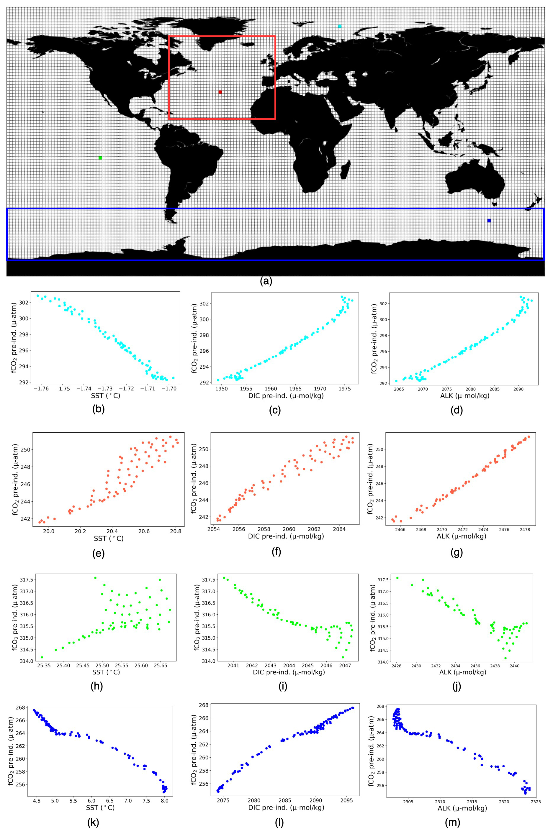
Figure A1 (a) 2°×2° boxes used for computing multivariate linear regressions, with the contours indicating the two basins – the North Atlantic and Southern Ocean – used for the detailed analysis in Sect. 3.2. The North Atlantic basin lies between 75–0° W and 10–70° N, and the Southern Ocean is between 45–77° S. (b–m) Scatter plots of fCO₂ against SST (b, e, h, k), DIC (c, f, i, l), and ALK (d, g, j, m) over the four boxes indicated as colors in panel (a).

Appendix B: Cluster selection based on BIC scores

B1 Normalized input for adaptive clustering

The inputs to the clustering algorithm are the normalized regression coefficients. Clustering algorithms are sensitive to the scale of variables. Variables with larger scales can dominate the grouping procedure and distort the results (Han et al., 2011). Normalizing variables ensures that all variables contribute equally to the agglomeration process, regardless of their original scales. Additionally, normalized data can lead to more meaningful clusters by focusing on relative differences between data points rather than absolute values. This gives us clusters that better capture the underlying structure of the data and are easier to interpret.

B2 BIC scores

BIC is a statistical measure utilized for model preference. BIC is based on the likelihood function and penalizes models for complexity to avoid overfitting. The BIC score for each clustering solution c (where |c| is the total number of clusters found) is computed using Eq. (B1):

$$\begin{array}{}\text{(B1)}& \mathrm{BIC}=-\mathrm{2}\cdot \mathrm{\Sigma }\log \left(\mathrm{likelihood}\right(c\left)\right)+\log \left(n\right)\cdot k,\end{array}$$

where log (likelihood) is the natural logarithm of the likelihood of the data per cluster c, k is the number of parameters or degrees of freedom in the model, and n is the number of data points. The likelihood measures how well the clusters explain the observed data. BIC comprises a penalty term for the number of parameters (in our case, three). This penalty term discourages overly complex models and helps prevent overfitting. The clustering solution with the lowest BIC score is chosen as the optimal solution. Lower BIC scores indicate a better trade-off between model fit and model complexity.

If we had cut the dendrogram using a global parameter, we would have ended up with either too much fragmentation at subpolar and high latitudes (e.g., selecting a distance of 20) or too little structure (e.g., a cut at 40). Using the adaptive method delineated in Sect. 2.3, we achieve a reasonable number of clusters reflective of their underlying data structure. We rely on BIC scores to select a pair of ΔDist and ΔVar. BIC scores can be used in clustering to determine the optimal number of groups by comparing the fit of different cluster solutions. First, the output of the distance–variance cluster selection methodology for different combinations of ΔDist (ranging from 20 to 30) and ΔVar (ranging from 0 to 1.0) is determined. For each selection, we receive a different number of clusters. Second, the likelihood of the input data (regression coefficients of the drivers) given the model is calculated for each clustering scenario.

We conducted 16 experiments for regression coefficients of January 2009 with different parameter choices as shown in Table B1. The clusters obtained through these pairs of ΔDist and ΔVar have between 40 and 100 BIC scores. These experiments show that the BIC scores decrease as ΔDist increases. With ΔDist=20.0 and ΔVar=0.1, we get nine clusters with the highest BIC scores (this implies a clustering model with higher complexity and overfitting). With ΔDist=30.0 and ΔVar=1.0, we get the lowest BIC scores, but the number of carbon uptake provinces is three, i.e., too low. We also see that for ΔDist=25.0, 28.0, and 30.0 and ΔVar=0.1, we get a comparatively lower BIC score and seven clusters. We opted for ΔDist=25.0 and ΔVar=0.1, as we can already distinguish distinct clusters with the lowest difference in the distance with the fixed difference in variance. We selected the clustering solution with the low BIC score to find the simplest model that best fits the data. BIC scores help identify the optimal number of clusters that effectively capture the underlying structure of the data without overfitting. These scores provide a principled approach to model selection in clustering, balancing goodness of fit and model complexity.

Table B1 Cluster (carbon biomes) selection for January 2009. BIC scores calculated over different combinations of clustering parameters ΔDist and ΔVar for hierarchical clustering on normalized regression coefficients of SST, DIC, and ALK. The parameter values of ΔDist and ΔVar in bold were selected for January 2009, which resulted in seven carbon biomes.

Appendix C: Visualization of shifting biomes between January and December in 2009

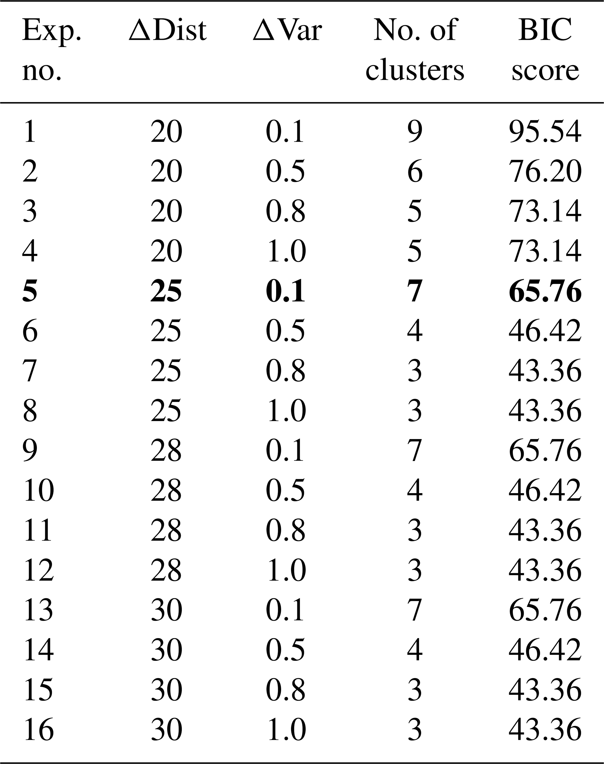
Figure C1 highlights how the carbon regimes detected in January 2009 have spatially evolved in the following 11 months. The dendrogram map (Fig. C1a) has all seven clusters detected. The maps (Fig. C1b to l) have six clusters or carbon biomes, as predicted by the FNN model.

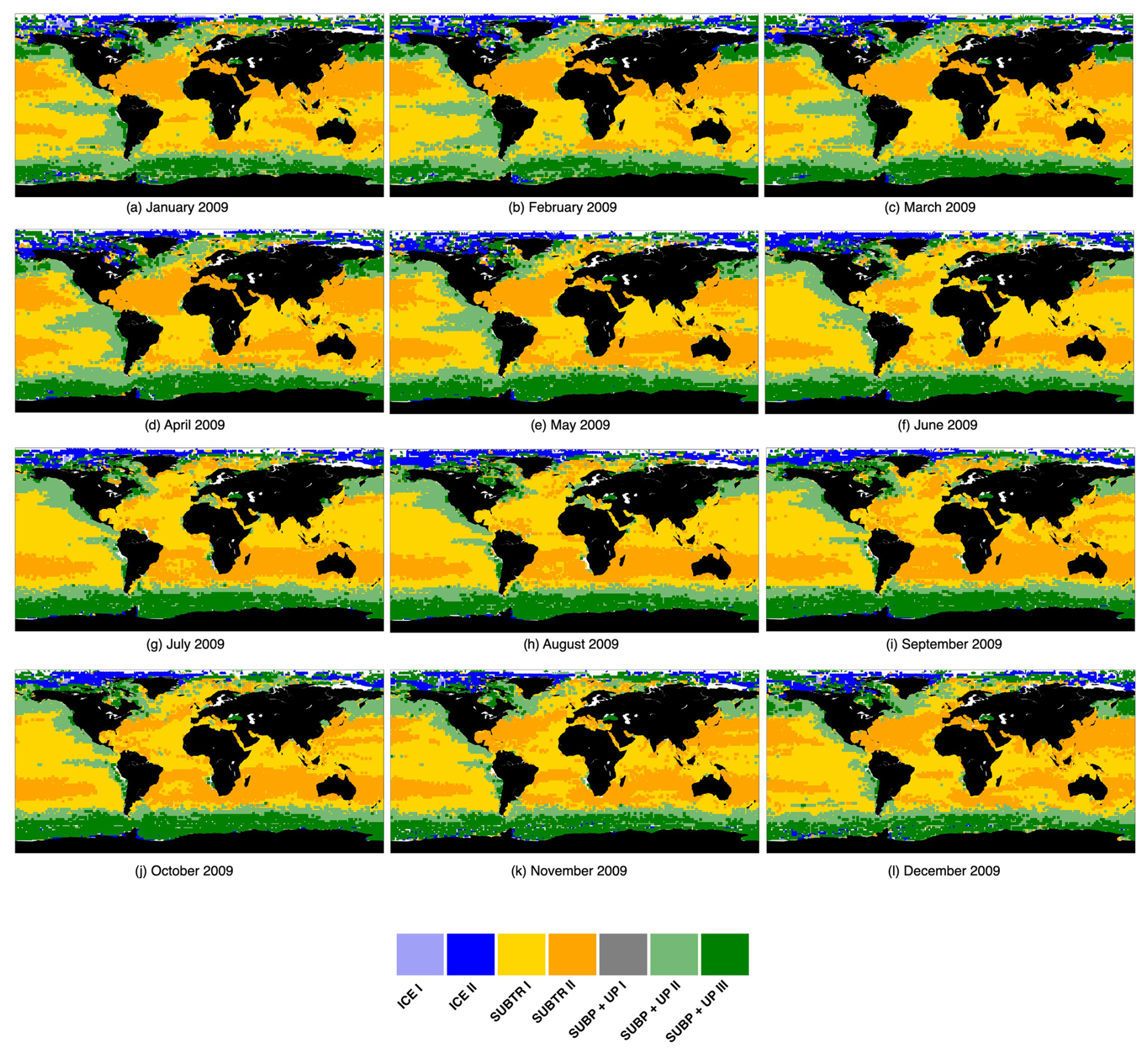
Figure C1 Carbon biomes over 12 months in 2009. The map in panel (a) is the outcome of the adaptive hierarchical clustering algorithm, while the maps in (b)–(l) are the output of the FNN model.

Appendix D: FNN model construction and evaluation

There are different components of implementing FNNs – activation functions, loss functions, optimizers, and evaluation criteria. Activation functions are an integral part of neural network construction. We have chosen the rectified liner unit (ReLU) for our input and hidden layers. The function returns the input value itself if it is positive. It returns 0 if the input value is negative. This has been shown in Eq. (D1). Depending on the outcome, the FNNs learn the importance of one variable (in our case, coefficients of SST, DIC, and ALK) over the others while predicting the biome labels. ReLU allows the network to learn more informative and discriminative features from the input data, producing enhanced performance. It provides nonlinearities without the vanishing gradient issue compared with sigmoid or tanh activation functions. This enables faster learning and better optimization of the model parameters.

$$\begin{array}{}\text{(D1)}& f\left(x\right)=\max (\mathrm{0},x)\end{array}$$

Our task is tracking the carbon biomes; i.e., the goal is to classify a set of regression coefficients into a particular cluster label. Thus, for the final layer in our FNN model, we use the softmax function. Softmax is well-suited for our multi-class classification task, as its objective is to provide one of several mutually exclusive cluster labels to input target–driver relationship data. Softmax also provides individual probabilities for each label, capturing uncertainties if necessary. These probabilities convey the FNN model's confidence or certainty about each cluster and biome label, permitting a probabilistic interpretation of the predictions. We pair softmax (Eq. D2) with the cross-entropy loss function (Eq. D3), which measures the distinction between the predicted probability distribution and the actual distribution of cluster and biome labels. Mathematically, let $z=(z_{\mathrm{1}},z_{\mathrm{2}},\mathrm{\dots },z_k)$ be the vector of scores produced by the neural networks for K number of cluster labels. The softmax function is applied to each element of z to produce the vector of predicted probabilities over K classes; $\widehat{y}=({\widehat{y}}_{\mathrm{1}},{\widehat{y}}_{\mathrm{2}},\mathrm{\dots },{\widehat{y}}_K)$, as shown in Eq. D2:

$$\begin{array}{}\text{(D2)}& {\widehat{y}}_i={\displaystyle \frac{e^{z_i}}{\sum _{j=\mathrm{1}}^K{e}^{z_j}}},\end{array}$$

where, $i=\mathrm{1},\mathrm{2},\mathrm{\dots },K$.

Let $y=(y_{\mathrm{1}},y_{\mathrm{2}},\mathrm{\dots },y_K)$ be the one-hot encoded vector for the actual cluster label (i.e., a vector with a 1 in the position corresponding to the true biome and 0 s elsewhere). The cross-entropy loss L between the predicted probabilities $\widehat{y}$ and the true labels y is computed as Eq. (C3):

$$\begin{array}{}\text{(D3)}& L(y,\widehat{\mathit{y}})=-\sum _{i=\mathrm{1}}^K{y}_i\log \left({\widehat{y}}_i\right),\end{array}$$

where $L(y,\widehat{y})$ is the cross-entropy loss, K represents the total number of class labels or cluster labels, $\widehat{\mathit{y}}$ is the vector representing the predicted probability distribution over the K clusters, ${\widehat{y}}_i$ is the predicted probability of class i, and y_i is the true probability of cluster label i (1 if the class is the true label and 0 otherwise).

FNNs also require an optimizer. An optimizer is an algorithm used to adjust the parameters (such as weights and biases) of the neural network during the training process. The objective of an optimizer is to minimize the loss function, which measures the difference between the predicted cluster label of the neural network and the actual cluster label. These optimizers help the neural network learn the fundamental patterns in the data and improve its performance by iteratively adjusting the parameters based on the gradient of the loss function. We employ ADAM (adaptive moment estimation) (Kingma and Ba, 2017) in our cluster prediction and tracking task. It is an adaptive learning rate optimization algorithm that combines the advantages of two other popular optimizers: AdaGrad (Duchi et al., 2011) and RMSProp (Ruder, 2016). ADAM speeds up the training process and improves generalization performance (i.e., lowered overfitting). The evaluation metrics used in our FNN model – accuracy (in percentage), precision, and recall – are defined as Eqs. (D4)–(D6), respectively.

$$\begin{array}{}\text{(D4)}& {\displaystyle }& {\displaystyle }\mathrm{Accuracy}={\displaystyle \frac{\mathrm{no}.\mathrm{of}\mathrm{correctly}\mathrm{predicted}\mathrm{instances}}{\mathrm{total}\mathrm{no}.\mathrm{of}\mathrm{instances}\mathrm{in}\mathrm{the}\mathrm{dataset}}}\times \mathrm{100}\text{(D5)}& {\displaystyle }& {\displaystyle }\mathrm{Precision}={\displaystyle \frac{\mathrm{true}\mathrm{positives}}{\mathrm{true}\mathrm{positives}+\mathrm{false}\mathrm{positives}}}\text{(D6)}& {\displaystyle }& {\displaystyle }\mathrm{Recall}={\displaystyle \frac{\mathrm{true}\mathrm{positives}}{\mathrm{true}\mathrm{positives}+\mathrm{false}\mathrm{negatives}}}\end{array}$$

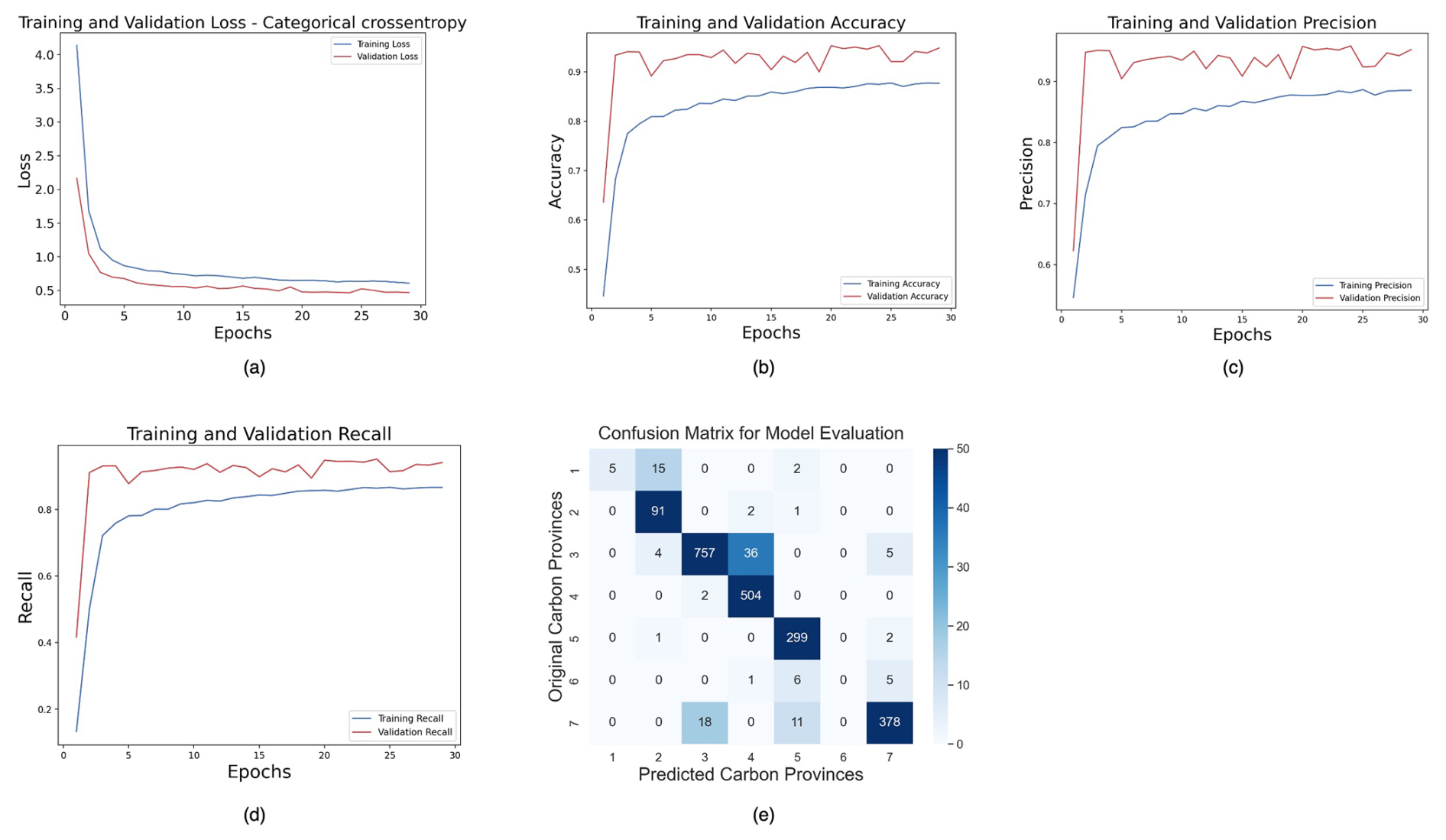
Figure D1 FNN model evaluation: during the training process, we used cross-entropy loss (a), accuracy (b), precision (c), and recall (d) to evaluate the quality of the model. The heatmap (e) is the confusion matrix plotted on a test set from January 2009 regression coefficients. In the confusion matrix, the numbers 1 to 7 represent the carbon biomes – 1: ICE I, 2: ICE II, 3: SUBTR I, 4: SUBTR II, 5: SUBP+UP III, 6: SUBP+UP I, and 7: SUBP+UP II.

During the experimentation, we first fixed the architecture with the number of layers being six (a relatively small number given the number of input features, i.e., three slopes) and the number of neurons per layer being 64, 128, and 256 (a standard practice in the ML community to choose neurons as a power of 2) to conduct sensitivity analysis for the hyperparameters (optimizer, learning rate, batch size, number of epochs, etc.) used in the neural network architecture. We have utilized a five-cross-validation technique for this analysis. Second, to understand how the model complexity could affect the outcome, we kept the hyperparameters constant and attempted to alter the neural network architecture by removing or adding a hidden layer, which resulted in a decrease or nonsignificant increase in test loss and accuracy (not shown).

To optimize and select a robust feed-forward neural network (FNN), we aimed to recognize the most constructive amalgam of hyperparameters that would maximize the predictive accuracy, precision, and recall of the deep learning model. Hence, we experimented with various hyperparameter configurations, including diverse batch sizes, optimizers, learning rates, and numbers of training epochs. We evaluated 16, 32, and 64 batch sizes with optimizers such as ADAM and stochastic gradient descent (SGD) with learning rates of 0.01 and 0.001. Additionally, we extended the number of training epochs from 50 to 200 to determine the influence of training duration on model performance. In totality, we ran 240 experiments, and the list of different combinations of hyperparameters can be found on our GitHub link.

Through this tuning process, we observed that the ADAM optimizer attained the highest test accuracy of 95.9 % over 50 epochs with a batch size of 32 and a learning rate set to 0.01. We employed early stopping to prevent overfitting, leading to the FNN being trained for 30 epochs. Figure D1 highlights how well the neural network was trained, and the plot in Fig. D1 emphasizes the change in cross-entropy loss during training and validation. The plots in Fig. D1b–e show how accuracy, precision, and recall, respectively, evolved during training and validation over the 30 epochs. The confusion matrix in Fig. D1e highlights the average test accuracy as 94.83 %, precision as 95.39 %, and recall as 94.5 % over seven different clusters.

D1 Limitations behind tracking SUBP+UP I

Our FNN model incorporated RC_SST, RC_DIC, and RC_ALK as inputs, with the target being the aforementioned carbon regimes. The distribution of labeled regimes across 2°×2° grid boxes is as follows: ICE I (1.03 %), ICE II (4.39 %), SUBTR I (37.40 %), SUBTR II (23.60 %), SUBP+UP I (0.55 %), SUBP+UP II (18.97 %), and SUBP+UP III (14.06 %). This indicates an inconsistent distribution of inputs among different labels in our FNN. The trained FNNs were subsequently employed to predict the seven regimes for 12 months over a span of 61 years (1958–2018). Notably, the prediction and tracking process successfully predicted six regimes, excluding SUBP+UP I. Such behavior in FNNs can arise from training on an imbalanced dataset, leading to a bias toward majority biome labels. In Fig. 3a, the RCs of SUBP+UP I exhibit closer proximity to SUBP+UP II, with their combination occurring at a very low Euclidean distance, suggesting minimal variation in the underlying distribution of both biomes. Furthermore, the combination of SUBP+UP I and SUBP+UP II lies closer to SUBP+UP III. As a result, the FNN model struggled to discern the structure of SUBP+UP I due to the scarcity of data points, leading it to associate the underlying RCs more strongly with SUBP+UP II and SUBP+UP III, which exhibit closer proximity in terms of RC distributions. The confusion matrix (Fig. D1e) illustrates the test predictions from January 2009, revealing that biome SUBP+UP I was predominantly predicted to be SUBP+UP II or SUBP+UP III.

Appendix E: Trends and correlations

Table E1 Correlations among biomes in North Atlantic (NATL) and Southern Ocean (SO) basins along with their respective trends. For each month over 49 years (1970–2018), we calculated the (i) correlations between SUBTR I and II in NATL, (ii) individual trend coefficients of SUBTR I and II in NATL, (iii) correlations between SUBP+UP II and III in SO, and (iv) individual trend coefficients of SUBP+UP II and III in SO. Note that the individual trend coefficient here represents the trend per decade. All statistically significant figures with p values less than 0.04 are highlighted in bold.

Appendix F: Trend of observational sea surface temperature

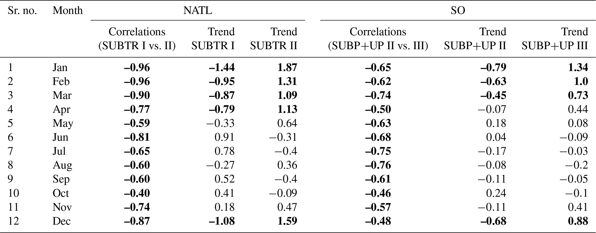
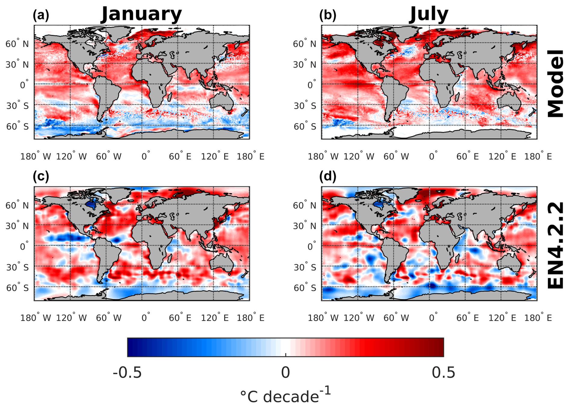
Figure F1 Change in SST between 1970–1970 and 2009–2018 in the model and in the EN4.2.2 observation-based product (Good et al., 2013). (a, b) Model and (c, d) EN4.2.2 product for (a, c) January and (b, d) July. The trend value in degrees Celsius (°C) per decade has been computed by dividing the SST difference by the number of years separating the median years of the two decades (i.e., 39 years) and multiplying by 10.

Appendix G: Comparison between simulated and observed climatologies of physical variables

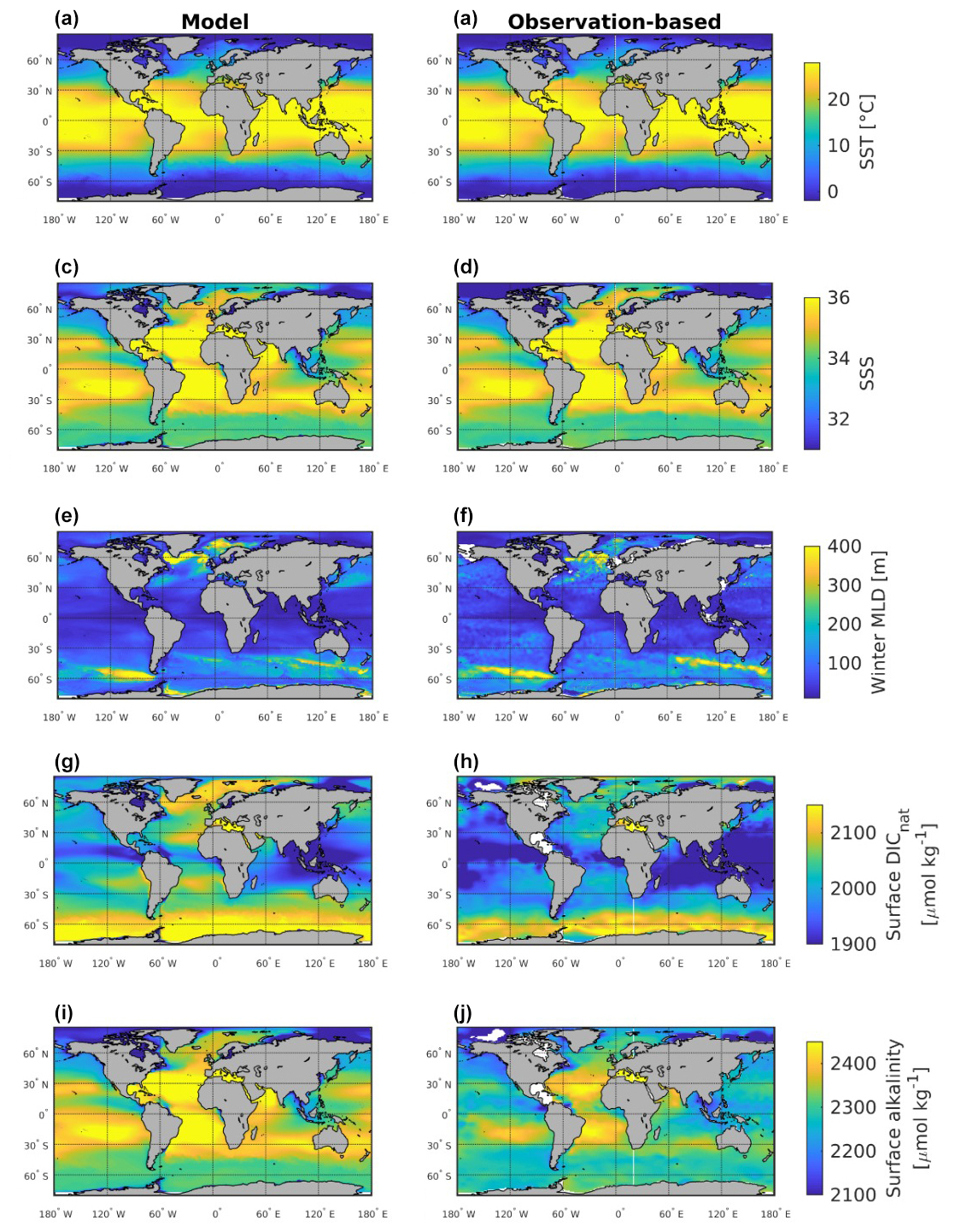
Figure G1 Comparison of simulated and observed climatologies of (a, b) sea surface temperature (SST), (c, d) sea surface salinity (SSS), (e, f) mixed layer depth (MLD) in March for the Northern Hemisphere and in September for the Southern Hemisphere, (g, h) natural (or pre-industrial) surface dissolved inorganic carbon (DIC), and (i, j) surface alkalinity. Observational estimates are from Good et al. (2013) for SST and SSS, Sallée et al. (2021) for MLD, and the GLODAPv2 2016 release (Lauvset et al., 2016) for pre-industrial DIC and alkalinity. The 2000–2018 climatologies for all variables except MLD are shown, for which a 1970–2018 average was computed (in accordance with the observational dataset).

Appendix H: Choice of January 2009 for biome detection

The choice of January and the year 2009 was random in our study, but this random choice is not expected to make a difference in the biome outcome. Figure H1 shows the kernel density distribution (KDE) of the regression coefficients (RCs) for some random years and the mean and standard deviation of RCs corresponding to each tracked biome computed over the 12 months of each year between 1958 and 2018. The KDE plot is a nonparametric way to estimate a continuous probability density function of the random variable. It is utilized to depict the distribution of data points in a smooth curve, which assists in comprehending the underlying data distribution.

The new analysis indicates that the RC kernel density distribution shows only subtle changes from year to year. The RCs within each biome (except for the strongly variable ICE biomes) are substantially stable overall in months and years. This stable behavior of the RCs over single biomes suggests that the specific month and year selected to build labels through hierarchical clustering should not affect the results. Instead, we argue that the leading subjective choice is the choice of the parameters used to cut the dendrogram resulting from the hierarchical clustering. The parameter choice yields a different degree of fragmentation or aggregation of the resulting clusters (not shown). We do not consider this a caveat because a different amount of aggregation and fragmentation may be desired depending on the user-defined application. However, once the labels are defined, we reason that the neural network can consistently track the different RC combinations in each detected biome.

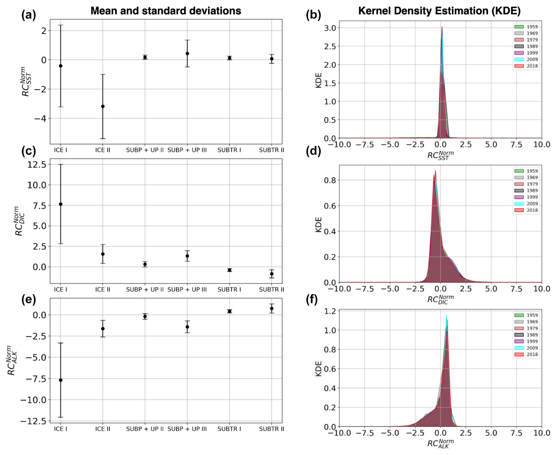
Figure H1 Distribution of normalized regression coefficients (RCs) resulting from the MVLR between fCO₂ and its drivers, i.e., (a, b) SST, (c, d) DIC, and (e, f) ALK. (a, c, e) Mean RCs over each of the six tracked biomes: ICE I, ICE II, SUBP+UP II, SUBP+UP III, SUBTR I, and SUBTR II. The mean and standard deviation are shown over the 12 months between 1958 and 2018. (b, d, f) Kernel density estimation (KDE) of normalized RCs over selected years. The KDE plot estimates the probability density function (PDF) of a continuous random variable, in our case the RCs, and visualizes the distribution of data points in a smooth curve, which helps to understand the underlying data distribution.