Impact of internal tides on chlorophyll a distribution and primary production off the Amazon shelf from glider measurements and satellite observations

The ocean region off the Amazon shelf including the shelf break presents a hotspot for internal tide (IT) generation, yet its impact on phytoplankton distribution remains poorly understood. While previous studies have extensively examined the physical characteristics and dynamics of ITs, their biological implications – particularly in nutrient-limited environments – remain underexplored. To address this question, we analyzed a 26 d glider mission deployed over September–October 2021 sampling hydrographic and optical properties (chlorophyll a) at high resolution along an IT pathway as well as satellite chlorophyll a and altimetry data to assess mesoscale interactions. Chlorophyll a dynamics were analyzed under varying IT intensities, comparing strong (HT) and weak (LT) internal tide conditions. Results reveal that ITs drive vertical displacements of the deep chlorophyll maximum (DCM) from 15 to 45 m, accompanied by 50 % expansion in its thickness during HT events. This expansion is observed with a dilution of the chlorophyll a maximum concentration within the DCM depth. While direct turbulence measurements were not collected, the observed vertical redistribution of chlorophyll a is indicative of tidally driven cross-isopycnal exchanges, the only physical mechanism explaining the transfer of biomass above and below the DCM. At the surface, turbulent fluxes provide 38 % of the chlorophyll a input, while the remainder is supplied by in situ biological activity. Notably, total chlorophyll a in the water column increases by 14 %–29 % during high internal tide phases, indicating a net enhancement of primary productivity driven by the combined effects of vertical mixing and stimulated surface-layer biological activity. These findings indicate that internal tides can be an important driver of chlorophyll a distribution and short-term biological variability in our study region. By reshaping the vertical chlorophyll a profile through vertical mixing, active internal tides influence primary productivity and may contribute to carbon cycling, particularly in oligotrophic oceanic environments where both a deep chlorophyll maximum and strong internal tides are present.

1 Introduction

Internal tides (ITs), also known as baroclinic tides, are ubiquitous in stratified oceans. These waves cause vertical displacements of isopycnal layers on the order of tens of meters and can propagate over long distances, reaching up to thousands of kilometers along the thermocline for the lowest modes (Zhao et al., 2016). Baroclinic tides are generated through the interaction of barotropic tidal currents with prominent submarine topographies such as continental slopes and mid-ocean ridges (Baines, 1982; Egbert and Ray, 2001; Munk and Wunsch, 1998). Internal solitary waves (ISWs) are highly stable internal waveforms that can propagate over long distances with a crest of a few tens of kilometers and are generally structured with a wave train trailing behind the main crest (Alford et al., 2015; Jackson et al., 2012; Jeans and Sherwin, 2001). The generation mechanisms and evolution of ISWs have attracted considerable attention in recent decades (Bai et al., 2021; Buijsman et al., 2010; Raju et al., 2021; Yuan et al., 2023). Their occurrence often serves as a direct indicator of the presence and nonlinear evolution of internal tides. ISWs are most commonly formed through the nonlinear transformation of internal tides (ITs) as they evolve (Grimshaw, 2003; Grisouard et al., 2011; Farmer et al., 2009; Zhang et al., 2018). More recently, river plumes have been identified as a source of ISWs in stratified coastal regions, where the density fronts generated by freshwater outflows can trigger wave generation. Examples include the Douro River plume off the Portuguese coast (Mendes et al., 2021), the Rhine River plume in the southern North Sea (Rijnsburger et al., 2021), and the Mzymta River plume in the Black Sea (Osadchiev, 2018). As they propagate, internal tides (ITs) and, to a lesser extent, internal solitary waves (ISWs) can break, releasing energy and inducing vertical turbulent mixing, with ITs often representing the dominant source of such mixing in stratified coastal and shelf seas (Alford et al., 2015; Lamb and Xiao, 2014; Moum et al., 2003; Nash et al., 2004). This mixing can play a crucial role in general circulation, contributing to the enclosure of the Atlantic Meridional Overturning Circulation (AMOC), and influencing oceanic energy and heat fluxes (Kantha and Tierney, 1997; Kunze, 2017; Waterhouse et al., 2014). Furthermore, because this mixing occurs close to the surface, it can influence climate variability through air–sea interactions. By altering sea surface temperature, it can modulate atmospheric convection, humidity, and precipitation patterns, as observed in the Indonesian seas, where IT-induced mixing leads to surface cooling and reduced rainfall (Koch-Larrouy et al., 2010; Sprintall et al., 2014).

While the physical characteristics of ITs have been extensively studied, their impact on biogeochemical processes remains relatively poorly explored (Holligan et al., 1985; Liu et al., 2006; Ma et al., 2023; Zaron et al., 2023). Their influence on plankton dynamics is of significant interest, as phytoplankton constitutes the lowest trophic level of marine ecosystems. Through photosynthesis and organic carbon production, phytoplankton regulates primary productivity and influences global biogeochemical cycles (Falkowski and Knoll, 2007). The spatial and temporal variability in phytoplankton populations is driven by a combination of biological factors, such as production and grazing, and physical processes, including ocean currents, mesoscale structures (fronts and eddies), and heat fluxes (Mahadevan and Campbell, 2002; Van Gennip et al., 2016). Given the timescale and amplitude of disturbances generated by ITs, it is reasonable to hypothesize that ITs can significantly influence phytoplankton distribution.

The effects of ITs on phytoplankton could occur through, at least, two primary mechanisms. First, vertical mixing induced by ITs can enhance nutrient fluxes into the euphotic zone, stimulating primary production and increasing phytoplankton biomass in regions with high IT activity (Bourgault et al., 2011; Capuano et al., 2025; Horne et al., 1996; Kaneko et al., 2025; Law et al., 2003; Lewis et al., 1986; Martin et al., 2010; Tsutsumi et al., 2020; Tuerena et al., 2019; Zaron et al., 2023). Second, the vertical displacements associated with ITs can alter the light and nutrient conditions experienced by phytoplankton cells near the pycnocline, thereby influencing their physiological responses and community structure (Gaxiola-Castro et al., 2002; Holloway and Denman, 1989; Jacobsen et al., 2023; Kahru, 1983; Lande and Yentsch, 1988; Sangrà et al., 2001; Vázquez et al., 2009)

The Amazon shelf break is recognized as a hotspot for internal tide (IT) generation, dissipation, and interactions with intense mesoscale features. First identified by Baines (1982), subsequent studies have confirmed its role in converting barotropic energy into baroclinic waves (Assene et al., 2024; Brandt et al., 2002; de Macedo et al., 2023; Ivanov et al., 1990; Magalhaes et al., 2016; Tchilibou et al., 2022; Vlasenko et al., 2005). However, the specific impacts of these ITs on biological processes off the Amazon shelf, particularly phytoplankton dynamics in the region, remain poorly understood and require further investigation.

This region (Fig. 1), situated in the western tropical Atlantic near the mouth of the Amazon and Pará rivers, features a shallow continental shelf and a macrotidal regime predominantly influenced by the semi-diurnal M₂ tidal component (Beardsley et al., 1995; Gabioux et al., 2005). The Amazon River significantly shapes local oceanographic conditions by modifying salinity, temperature, and water column stratification (Geyer, 1995; Ruault et al., 2020). During the August–September–October (ASO) season, reduced river discharge leads to a weaker and deeper pycnocline, along with a stronger North Brazil Current (NBC) and higher eddy kinetic energy (EKE) (Neto and Da Silva, 2014; Silva et al., 2005; Tchilibou et al., 2022). The isopycnal layers are thicker nearshore and become tighter offshore, causing weaker coastal stratification that increases offshore. These seasonal variations clearly highlight the dynamic shifts in vertical density gradients, consistent with observations by Aguedjou et al. (2019), making the ASO season an optimal period for investigating internal tides in the region.

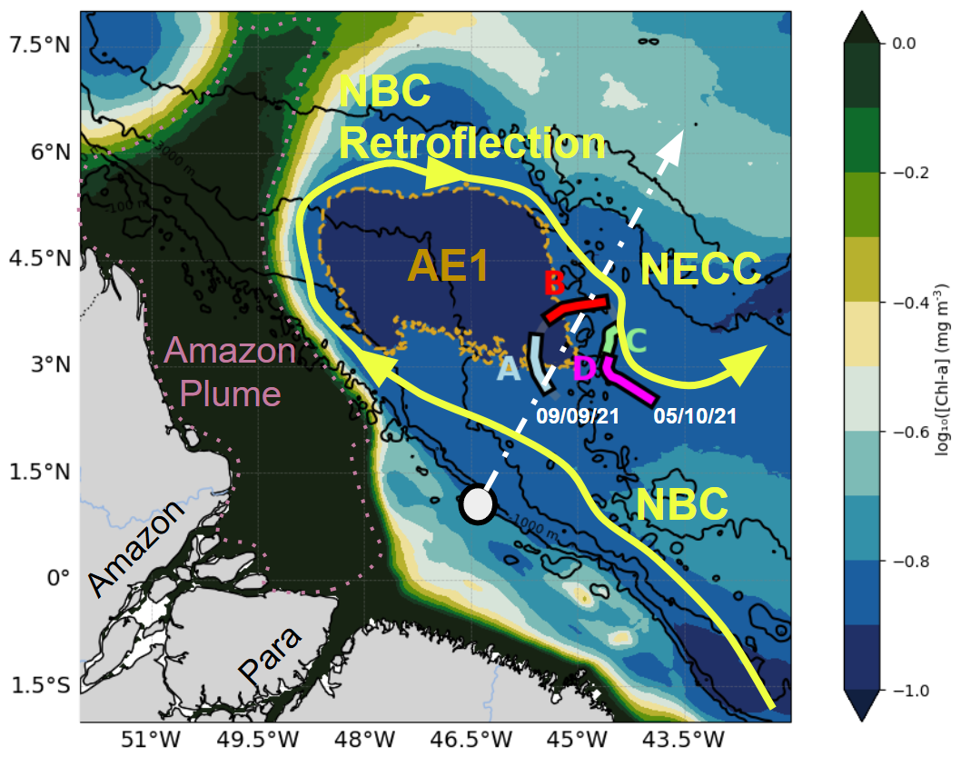
Figure 1 Chlorophyll map averaged between 9 September and 5 October 2021 in the glider deployment region, divided into four subregions: A (blue), B (red), C (green), and D (magenta), each characterized by distinct temperature–salinity (T/S) properties (Sect. 3.1). The yellow area marks the main surface current, purple indicates the plume, and light brown highlights AE1, the anticyclonic eddy detected by altimetry during the transect. The dashed white line shows the main internal tide propagation pathways identified by Magalhães et al. (2016) and Tchilibou et al. (2022), while the gray circle marks the primary internal tide generation site (0.75° N, 46° W).

The dynamics of this region are further shaped by interactions with the NBC, a major western boundary current transporting warm, saline waters from the South Atlantic (Garzoli et al., 2003; Johns et al., 1998; Schott et al., 1998; Silva et al., 2005). Between June and February, the NBC undergoes a seasonal retroflection, forming large anticyclonic rings that propagate northwestward (Fratantoni and Richardson, 2006; Fratantoni and Glickson, 2002). These anticyclonic eddies, known as “NBC rings”, can modulate stratification and nutrient distributions, influencing phytoplankton productivity (Mikaelyan et al., 2020). During the second part of the year a large part of the NBC retroflects to feed the eastward North Equatorial Countercurrent (NECC) (Dimoune et al., 2023).

To investigate the role of ITs in-shaping phytoplankton dynamics in the oceanic region off the Amazon shelf, the AMAZOMIX cruise aimed to collect a wide range of in situ measurements. Conducted between September and October 2021 – an optimal period for IT activity and mesoscale interactions – the cruise employs a multi-faceted approach combining numerical models, satellite data, and in situ observations. In addition to ship-based measurements, an autonomous underwater glider was deployed from 9 September to 5 October 2021 to have high-resolution vertical structure data (hydrographic and chlorophyll a) influenced by ITs.

The objective of this study is to investigate how ITs influence the vertical distribution of chlorophyll a concentration off the Amazon shelf. Analyses were performed by examining glider measurements and remote sensing observations and by comparing periods of strong and weak internal tide activity under similar stratification conditions.

2 Data and methods

2.1 Data

2.1.1 Autonomous glider

On 9 September 2021, during the AMAZOMIX campaign an autonomous underwater glider (Testor et al., 2019) was deployed for 26 d (9 September to 5 October 2021) between the NBC and NECC, the adjacent oceanic waters off northern Brazil (Fig. 1) in the core of an IT propagation path identified by Magalhaes et al. (2016) and Tchilibou et al. (2022). A Slocum G2 glider from Teledyne Webb Research was used, which is able to dive to 1000 m within 4 h and to cover approximately 20 km d⁻¹ horizontally relative to the water, assuming optimal conditions and no currents. Due to strong currents near 1 m s⁻¹ representing a real challenge for glider operation, the glider only completes a total distance of 513 km over the ocean during the 26 d deployment. The glider was equipped with a Seabird pumped CTD (temperature, pressure, conductivity), an Aanderaa optode (dissolved oxygen), and a WetLabs optical puck (chlorophyll a fluorescence, CDOM, and turbidity). The sensors had a sampling frequency of 5 s, resulting in a vertical sampling interval of approximately 1 m. Between each surfacing, the glider estimates its position using navigation sensors (compass) allowing estimation of a mean dive-average horizontal currents while comparing its dead-reckoned position with GPS fixes. The glider dataset was processed using the Geomar MATLAB Toolbox (Krahmann, 2023), which includes the removal of thermal lag errors following (Garau et al., 2011). All scientific and system data were linearly interpolated to 1 s intervals, aligning science and navigation variables with the glider's main processor clock. The interpolation introduces minimal additional noise, as the vertical displacement of the glider over 1 s is typically < 0.2 m. In the vertical, data from each dive profile (denoted “yo”) were binned and averaged into 1 dbar intervals, and then interpolated linearly to produce uniformly gridded vertical profiles. These profiles were used in all subsequent analyses, including spectral decomposition, stratification diagnostics, and vertical chlorophyll characterization. After the standard GEOMAR gridding (1 dbar vertically and timestamp aligned), we applied a second linear interpolation in time to project the variables onto a common regular temporal grid. This interpolation was performed independently at each depth level using valid (non-NaN) observations, ensuring a complete and consistent 2D structure across depth and time. These interpolated matrices were used for spectral and variability analyses.

Temperature and salinity were converted to conservative temperature and absolute salinity using the Gibbs Seawater Python library (McDougall and Barker, 2011). The temperature and salinity profiles were validated by comparison with a reference CTD at the glider deployment site. Daytime chlorophyll a fluorescence profiles were corrected for non-photochemical quenching processes using the method described by Thomalla et al. (2018), setting the quenching depth at 40 m. To enable direct comparison with satellite-derived data, chlorophyll a concentrations measured by the glider were averaged from the surface down to the first optical depth (Zpd = Zeu / 4.6, Morel, 1988) to build the time series, which defines the depth range primarily sensed by ocean color remote sensors.

2.1.2 Remote sensing observations: ISW detection, chlorophyll a distribution, and mesoscale eddy tracking

Internal solitary waves (ISWs) create patterns alternating between rough and smooth surface areas, corresponding to convergent and divergent surface currents, respectively. Thus, their signatures in MODIS images during sunglint or in the SAR imagery are manifested by variations in sea surface roughness, resulting in changes in the brightness of the captured images (De Macedo et al., 2023; Jackson and Alpers, 2010; Magalhaes et al., 2016). During the cruise, ISW signatures were visually identified and manually extracted off the Amazon shelf from a representative assembled dataset composed of 21 remote sensing imagery acquired by active and passive sensors from 1 September to 10 October 2021. A total of 13 images were acquired by the synthetic aperture radar (SAR) C-band (center frequency of 5.4 GHz) Copernicus Sentinel-1A and 1B instruments Level-1 GRD (ground range detected) products in the interferometric wide swath mode with about 250 km of swath and spatial resolution of 20.3 × 22.6 m (range × azimuth), operating in single polarization (VV channel). The SAR imagery were collected from the Copernicus Open Access Hub (https://scihub.copernicus.eu/dhus/#/home, last access: 10 May 2025). The SAR scenes were pre-processed using the software SNAP and Sentinel Toolboxes (version 8.0) by calibrating the data (conversion from digital number to normalized radar cross-section) and applying a 5 × 5 boxcar filter to reduce the speckle noise. A total of eight Level-1B imagery sets were acquired by the Moderate Resolution Imaging Spectroradiometer (MODIS) sensor onboard the TERRA and AQUA satellites. Band 6 centered at 1640 nm with a spatial resolution of 500 m was used to identify the ISW signatures in the sun glint region. The MODIS/TERRA and AQUA imagery were collected from NASA's Earth Science Data System, ESDS (https://earthdata.nasa.gov/, last access: 10 May 2025).

Given that ocean color observations are often affected by interference from clouds, leading to data gaps, we used the daily mean merged chlorophyll a (with a spatial resolution of ∼ 4 km) product from the GlobColour project to maximize data coverage from 1 September to 5 October 2021 provided by the ACRI-ST company (Garnesson et al., 2019). This product provides chlorophyll a concentration information from the ocean color sensors MODIS-AQUA, NPP-VIIRS, NOAA20-VIIRS, and Sentinel-3 OLCI A and B, including updated ancillary information (i.e., meteorological and ozone data for atmospheric correction, and attitude and ephemerides for data geolocation). According to Garnesson et al., 2019, the approach merges three algorithms: (1) the CI approach for oligotrophic waters (Hu et al., 2012); (2) the OCx (OC3, OC4, or OC4Me depending on the sensor) approach for mesotrophic waters; and (3) the OC5 algorithm for complex waters (Gohin, 2011). The product can be found on the CMEMS website. In this study, we utilized data provided by GlobColour, specifically estimates of the euphotic depth (Zeu) derived from satellite observations of the MODIS-Aqua sensor. These Level-3 processed data are available at a spatial resolution of 4 km and were obtained from the GlobColour platform. The euphotic depth was estimated following the methodology described by Morel and Maritorena (2001), which is based on an empirical relationship linking surface chlorophyll a concentration to light penetration depth, which defines Zeu as the depth where incident light is reduced to 1 % of its surface value. The dataset is publicly available at HERMES ACRI.

Daily maps of the SSALTO/DUACS absolute dynamic topography (ADT) gridded product were used to identify and track coherent mesoscale eddies during AMAZOMIX campaign. This product was obtained from all available satellite altimetry along-track data and optimally interpolated onto 0.25° × 0.25° longitude × latitude (Pujol et al., 2016). Mesoscale eddies were identified using the algorithm developed by Chaigneau et al. (2009, 2008) and Pegliasco et al. (2015). In this method, an eddy is identified by its center and its external edge. The eddy center corresponds to a local extremum (maximum for an anticyclonic eddy and minimum for a cyclonic eddy) in ADT while the eddy edge corresponds to the outermost closed ADT contour around each detected eddy center. One long-lived anticyclonic eddy (AE1) was identified during the AMAZOMIX campaign. AE1 was generated within the study domain from instability of NECC and propagated northwestward, making the NECC oscillate the NBC Fig. 3. AE1 lasted for more than 120 d. The bathymetric data used in this study are sourced from the NOAA CoastWatch Program and are accessible through the NOAA CoastWatch Data Portal. These data are formatted for MATLAB and are stored under https://www.ncei.noaa.gov/maps/bathymetry/ (last access: 4 December 2024) and https://coastwatch.pfeg.noaa.gov (last access: 4 December 2024). The bathymetric dataset, referenced from Topography SRTM30 Version 6.0 (30 arcsec Global), provides detailed seafloor topography information crucial for analyzing oceanographic processes. Additionally, the geostrophic velocity data used in this study are sourced from the Global Ocean Gridded SSALTO/DUACS Sea Surface Height L4 product, provided by Mercator through the Copernicus Marine Service. This product includes surface geostrophic eastward and northward seawater velocities, calculated from sea surface height assuming sea level as the geoid reference. These data, derived from sea surface height, provide essential surface currents. The dataset is available via Copernicus Marine Data.

2.1.3 FES model

Tidal data were extracted from the global FES2014 (Finite Element Solution) model developed by Lyard et al. (2021). The outputs of the sea surface elevation field (eta) were used at the grid point corresponding to 0.75° N, 46° W, which corresponds to an internal tide generation site previously identified by Magalhaes et al. (2016) and Tchilibou et al. (2022). The use of those data helped us to identify neap tides and spring tides.

2.2 Methods

To assess the impact of ITs on the vertical distribution of chlorophyll a (hereafter referred as CHL for the equations), a multi-step approach was applied. (1) Satellite observations were used to characterize the large-scale spatial distribution of chlorophyll a and the physical processes influencing it, enabling the identification of hydrographically distinct regions (Sect. 3.1) (2) Based on this preliminary analysis, the glider data were divided into transects representing four periods (A, B, C, and D; Fig. 1; Sect. 3.2) with contrasting hydrographic properties. These periods were defined based on marked changes in temperature, salinity, and potential density structure, identified through visual inspection of vertical profiles and T–S diagrams, focusing on shifts in stratification patterns and salinity ranges across isopycnal layers. (3) Given the prevalence of ITs in the study area, periods A and B were further subdivided into low-tide (LT) and high-tide (HT) phases using spectral analysis of the temperature field to estimate tidal amplitude; the classification was based on the presence of a spectral peak at the M₂ frequency (Sect. 3.2). (1) Chlorophyll a fluorescence profiles collected by the glider were then averaged and statistically compared between LT and HT conditions to evaluate the effect of IT intensity on chlorophyll a vertical distribution (Sect. 3.3). (2) Finally, vertical turbulent fluxes of chlorophyll a were estimated to better understand the transport mechanisms associated with ITs (Sect. 3.3).

2.2.1 Temperature power spectra

We analyzed temperature time series between 145 and 165 m depth, where the largest vertical displacement of isotherms was observed. The high-frequency glider profiling (about 12 profiles per day) enabled the construction of temperature time series resolving the main tidal frequency (12 h). To compute the power spectra of temperature variability at this depth interval, all measurements within the 145–165 m range were treated equally, without vertical weighting and concatenated into a composite 1D time series. The resulting signal, sampled at irregular intervals due to glider motion, was interpolated onto a uniform time grid using pandas.resample(“1H”).mean().interpolate(), which performs hourly averaging followed by linear interpolation over missing values. This procedure ensures temporal regularity and allows consistent application of Fourier analysis. While no formal vertical averaging was applied, the method assumes that variability within the selected layer is coherent enough to be represented by a single aggregated signal. Prior to computing the spectra, a Hanning window was applied to the time series to reduce spectral leakage, zero-padding was used to increase frequency resolution, and a 10-point moving average was applied to the resulting power spectrum for clearer visualization. The aggregated time series was then detrended to remove long-term variations, and a fast Fourier transform (FFT) was applied to convert the time series into the frequency domain. The power spectrum was calculated to identify the dominant oscillation frequencies (McInerney et al., 2019).

2.2.2 Diapycnal chlorophyll flux estimation

The vertical dynamics of chlorophyll a concentration (CHL) in the water column is described by the following equation adapted from the vertically resolved NPZ formulation (Franks, 2002), with the physical transport term representing cross-isopycnal turbulent fluxes associated with internal tides:

$$\begin{array}{}\text{(1)}& \begin{array}{rl}{\displaystyle \frac{\partial \mathrm{CHL}(z,t)}{\partial t}}& +w{\displaystyle \frac{\partial }{\partial z}}\mathrm{CHL}(z,t)={\displaystyle \frac{\partial }{\partial z}}\left(K_z{\displaystyle \frac{\partial }{\partial z}}\mathrm{CHL}\right(z,t\left)\right)\\ & +\mathrm{SMS}(z,t),\end{array}\end{array}$$

where CHL is the chlorophyll a concentration. The $w\frac{\partial }{\partial z}\mathrm{CHL}\left(zt\right)$ term represents the vertical advection of chlorophyll by the vertical velocity field w, while $\frac{\partial }{\partial z}\left(K_z\frac{\partial }{\partial z}\mathrm{CHL}\left(z\right)\right)$ accounts for vertical turbulent diffusion, with K_z being the diffusivity coefficient. The source-minus-sink (SMS) term encompasses biological processes, specifically primary production and grazing, which regulate the net chlorophyll a balance in the system.

To isolate turbulent chlorophyll a fluxes, the analysis is conducted within a vertical isopycnal reference framework. In this context, the advection term $w\frac{\partial }{\partial z}\mathrm{CHL}\left(z\right)=\mathrm{0}$ as vertical velocities advect isopycnals up and down. By changing the vertical coordinate from z to ρ, $\frac{\partial \mathrm{CHL}\left(\mathit{\rho }\right(z\left)\right)}{\partial z}=\frac{\partial \mathit{\rho }}{\partial z}\frac{\partial \mathrm{CHL}\left(\mathit{\rho }\right(z\left)\right)}{\partial \mathit{\rho }}$, and assuming $\frac{\partial \mathit{\rho }}{\partial z}$ and K_z is constant leads to

$$\begin{array}{}\text{(2)}& {\displaystyle \frac{\partial \mathrm{CHL}(\mathit{\rho },t)}{\partial t}}=K_v{\displaystyle \frac{{\partial }^{\mathrm{2}}\mathrm{CHL}(\mathit{\rho },t)}{\partial {\mathit{\rho }}^{\mathrm{2}}}}+\mathrm{SMS}(\mathit{\rho },t),\end{array}$$

where the constant $K_v=(\frac{\partial \mathit{\rho }}{\partial z}{)}^{\mathrm{2}}{K}_z=(\frac{N^{\mathrm{2}}{\mathit{\rho }}_{\mathrm{0}}}{g}{)}^{\mathrm{2}}{K}_z$ represents the diapycnal diffusivity coefficient with ρ₀ the mean density of the ocean and g the gravitational acceleration. By integrating between two isopycnal density surfaces (ρ₀ and ρ₁), the average variations over a given period (ΔT) are defined as

$$\begin{array}{}\text{(3)}& <P{>}_{{\mathit{\rho }}_{\mathrm{0}},{\mathit{\rho }}_{\mathrm{1}},\mathrm{\Delta }T}={\displaystyle \frac{\mathrm{1}}{\mathrm{\Delta }T}}\underset{\mathrm{\Delta }T}{\int }\underset{{\mathit{\rho }}_{\mathrm{0}}}{\overset{{\mathit{\rho }}_{\mathrm{1}}}{\int }}{\displaystyle \frac{\partial P(\mathit{\rho },t)}{\partial t}}\mathrm{d}\mathit{\rho }\mathrm{d}t,\end{array}$$

where P corresponds to either $\frac{\partial \mathrm{CHL}(\mathit{\rho },t)}{\partial t}$ or $K_v\frac{{\partial }^{\mathrm{2}}\mathrm{CHL}(\mathit{\rho },t)}{\partial {\mathit{\rho }}^{\mathrm{2}}}$ or SMS(ρ,t) and $<P>$ to < CHL >, < DIFF > or < SMS >.

For two distinct periods corresponding to complete tidal cycles, HT forcing and LT forcing were defined within each observation window based on the relative intensity of internal tide activity. HT corresponds to the phase closer to spring tide conditions, characterized by stronger isopycnal displacements, while LT corresponds to the phase farther from spring tide conditions, with reduced vertical displacements. These definitions are relative within each observation window and account for local stratification conditions.

$$\begin{array}{}\text{(4)}& \mathrm{\Delta }{P}_{\mathit{\rho }\mathrm{0},\mathit{\rho }\mathrm{1},\mathrm{Tides}}=<P{>}_{\mathit{\rho }\mathrm{0},\mathit{\rho }\mathrm{1},\mathrm{HT}}-<P{>}_{\mathit{\rho }\mathrm{0},\mathit{\rho }\mathrm{1},\mathrm{LT}}\end{array}$$

The comparison between periods of strong (HT) and weak (LT) tidal forcing, relating to spring tides/neap tides cycle, conducted in a region with similar hydrodynamic properties but primarily differentiated by the intensity of ITs, served as a proxy for quantifying the influence of ITs on turbulent chlorophyll a fluxes.

We divided the water column into three isopycnal layers: the surface layer, the deep chlorophyll maximum (DCM) layer, and the bottom layer. We assumed that the difference in mean chlorophyll a integrated in an isopycnal layer around the DCM, defined here as ΔCHL_DCM, and the change in depth-integrated chlorophyll a, in mg m⁻², within the DCM layer attributable to turbulent diffusive fluxes are redistributed upward and downward through mixing such that their sum equals ΔDiff_DCM =ΔCHL_DCM, with proportions n for the surface layer and m for the bottom layer, where n+m = 1. This assumption is consistent with recent observations in our study area showing that internal tides dominate vertical mixing over the Amazon shelf break (Kouogang et al., 2025). Using this partitioning approach, we express the variation in chlorophyll a (ΔCHL) for each layer as follows:

$$\begin{array}{}\text{(5)}& {\displaystyle }\mathrm{\Delta }{\mathrm{CHL}}_{\mathrm{SURF}}=-n\cdot \mathrm{\Delta }{\mathrm{Diff}}_{\mathrm{DCM}}+\mathrm{\Delta }{\mathrm{SMS}}_{\mathrm{SURF}},\text{(6)}& {\displaystyle }\mathrm{\Delta }{\mathrm{CHL}}_{\mathrm{DCM}}=\mathrm{\Delta }{\mathrm{Diff}}_{\mathrm{DCM}}+\mathrm{\Delta }{\mathrm{SMS}}_{\mathrm{DCM}},\text{(7)}& {\displaystyle }\mathrm{\Delta }{\mathrm{CHL}}_{\mathrm{DEEP}}=-m\cdot \mathrm{\Delta }{\mathrm{Diff}}_{\mathrm{DCM}}+\mathrm{\Delta }{\mathrm{SMS}}_{\mathrm{DEEP}},\end{array}$$

with $-n\cdot \mathrm{\Delta }{\mathrm{Diff}}_{\mathrm{DCM}}=\mathrm{\Delta }{\mathrm{Diff}}_{\mathrm{SURF}}$ and $-m\cdot \mathrm{\Delta }{\mathrm{Diff}}_{\mathrm{DCM}}=\mathrm{\Delta }{\mathrm{Diff}}_{\mathrm{DEEP}}$.

By summing Eqs. (5), (6), and (7), the diffusion-related component cancels out, leaving

$$\begin{array}{}\text{(8)}& \mathrm{\Delta }{\mathrm{SMS}}_{\mathrm{DCM}}+\mathrm{\Delta }{\mathrm{SMS}}_{\mathrm{Surf}}+\mathrm{\Delta }{\mathrm{SMS}}_{\mathrm{Deep}}=\mathrm{\Delta }{\mathrm{CHL}}_{\mathrm{TOT}}.\end{array}$$

The total chlorophyll a variation ΔCHL_TOT between high-tide (HT) and low-tide (LT) periods is interpreted as follows: if ΔCHL_TOT > 0, this value represents the minimum possible net production. Similarly, if ΔCHL_TOT < 0, it indicates a dominance of grazing.

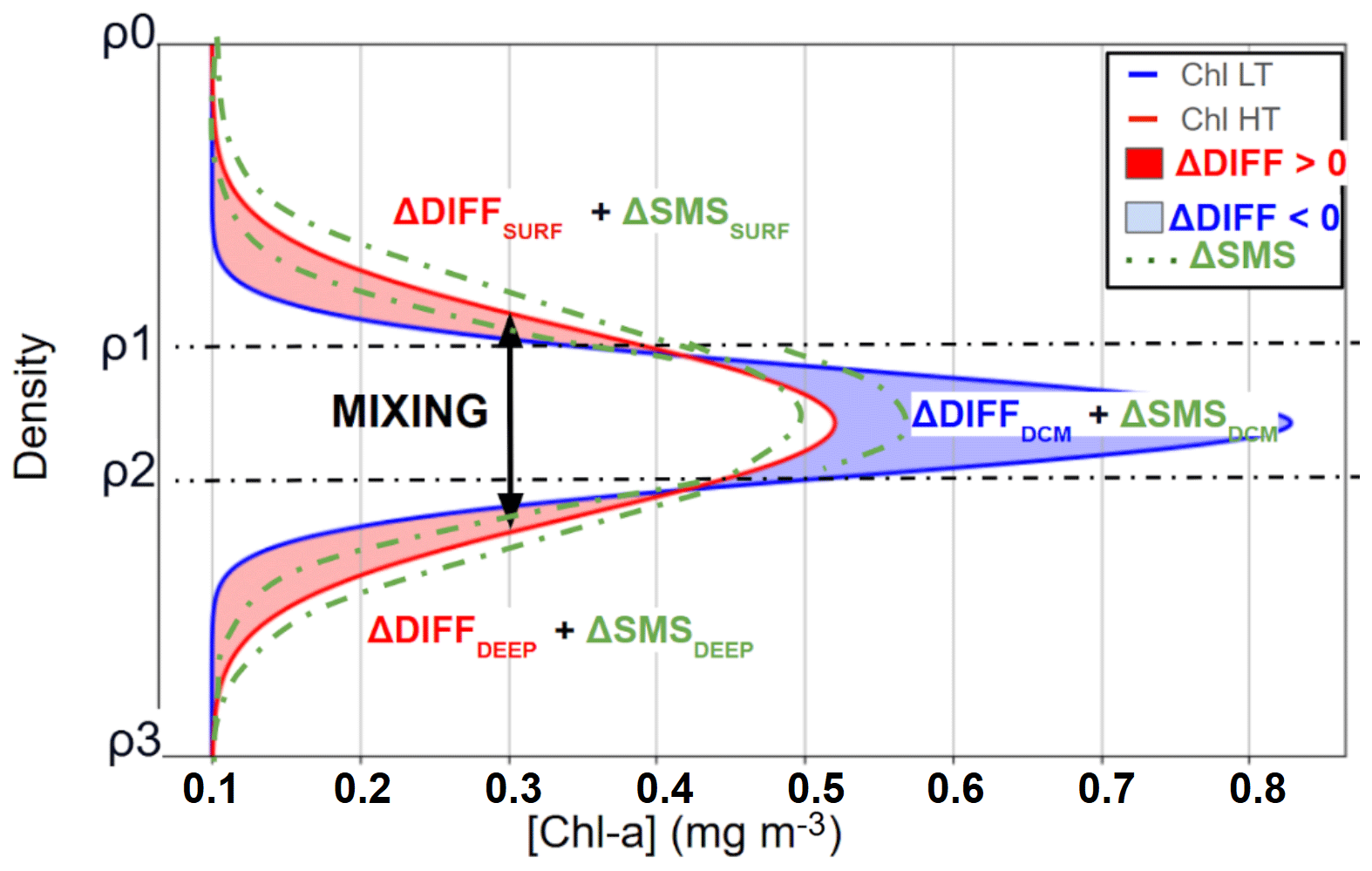
Figure 2 Schematic representation of vertical chlorophyll a distribution during low tidal forcing (LT, blue) and high tidal forcing (HT, red) periods, illustrating profile modifications induced by internal tide-driven mixing. Red shading (ΔDiff > 0) indicates chlorophyll a increases due to ITs mixing, blue shading (ΔDiff < 0) indicates decreases due to ITs mixing, and green shading denotes the potential range of variation in chlorophyll a attributable to SMS (biological sources and sinks), which can either increase or decrease chlorophyll a concentrations.

2.2.3 Statistical analysis

In this study, various statistical methods were employed to analyze the impact of ITs on chlorophyll a distribution across density layers. The Mann–Whitney U test, a non-parametric test, was selected to compare chlorophyll a concentrations between periods of high and low ITs within different density layers. This test is particularly suitable here, as it does not require the assumption of data normality distribution, which is often difficult to ensure for environmental samples with irregular distributions. Mean comparisons and percentage changes provide a statistical approach of ITs on chlorophyll a. Maximum chlorophyll a concentrations and DCM thickness were extracted from fluorescence profiles. A Spearman ranked correlation analysis was performed to assess the relationship between these variables. Statistical significance was determined using the associated p value. Additionally, descriptive statistics on the isopycnal layer were calculated for each density zone, offering a detailed view of trends specific to layers and enabling the identification of significant changes. Collectively, these methods robustly capture significant differences and their potential effects on chlorophyll a distribution and concentration.

3 Results

3.1 The glider study area

The oceanic circulation in the study area was dominated by two major current systems: the NBC and the NECC. Their interaction was regulated by the seasonal retroflection of the NBC, as that was clearly illustrated in the absolute dynamic topography (ADT) maps (Fig. 3a–d). This circulation was associated with ADT values reaching approximately 0.6 m. From a biogeochemical perspective, strong contrasts were observed between offshore waters and the continental Amazon shelf. The offshore waters were characterized by oligotrophic conditions, with low chlorophyll a concentrations (∼ 0.1 mg m⁻³), whereas the Amazon shelf was dominated by turbid waters, rich in suspended matter, with chlorophyll a concentrations exceeding 1 mg m⁻³ (Fig. 3e–h). This gradient highlighted the significant influence of the Amazon plume on local productivity. Moreover, the depth of the euphotic layer (Zeu; Fig. 4, purple) varied along the glider transect, showing a decrease in the eddy core and an increase toward its periphery, following a pattern similar to that observed for chlorophyll a.

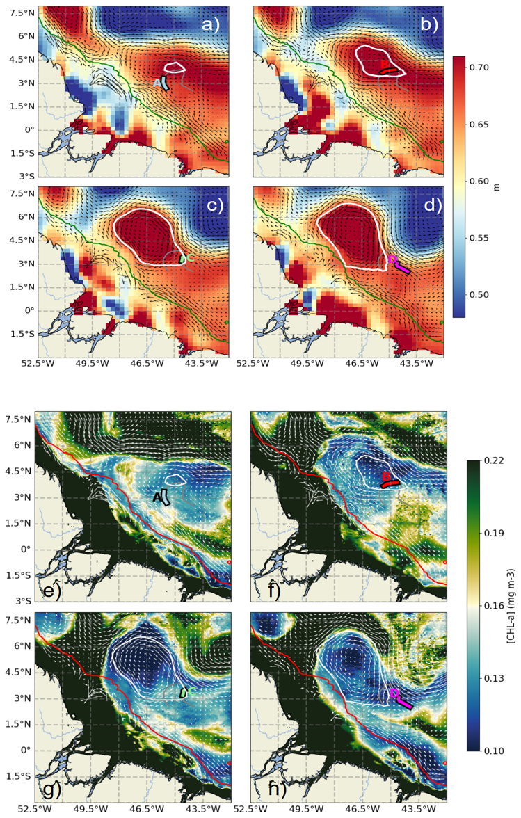
Figure 3 (a–d) Absolute dynamic topography (ADT) maps for 11 September (a), 16 September (b), 22 September (c), and 28 September (d) 2021. (e–h) Satellite-derived surface chlorophyll a maps for the same dates: 11 September (e), 16 September (f), 22 September (g), and 28 September (h). The AE1 eddy is outlined by white ovals. The glider trajectory is shown as a gray line, with color-coded segments indicating periods A, B, C, and D (as defined in Fig. 1). Geostrophic surface currents are shown as arrows. The 1000 m isobath is marked in green (a–d) and red (e–h).

3.1.1 Formation and evolution of the anticyclonic eddy (AE1)

On 11 September 2021, an anticyclonic eddy (AE1) formed in the region, identified by an ADT peak reaching approximately 0.7 m (Fig. 3a, white circle). The eddy core gradually migrated from 4° N, 44.5° W to 5.5° N, 47.5° W over the following 27 d, covering roughly 372 km with an average speed of 0.16 m s⁻¹. Between 12 and 19 September, the eddy underwent significant expansion, with its radius increasing from 100 km to approximately 400 km.

3.1.2 Glider–eddy interactions

The influence of the eddy on surface velocity is evident from an initial decrease in speed from 0.58 to 0.17 m s⁻¹ on 17 September, followed by a gradual acceleration reaching 0.8 m s⁻¹ at the end of the transect (Fig. 4, bottom panel). Between 14 and 22 September, as the glider traversed the eddy, variations in its distance from the eddy's outer boundary were observed (Fig. 4, top panel). These fluctuations confirm that the glider remained along the eddy's periphery, highlighting the kinematic effects induced by its circulation. Maximum geostrophic velocities, derived from ADT gradients, further indicate intense eddy dynamics, with circulating currents reaching up to 0.8 m s⁻¹ toward the end of the observation period.

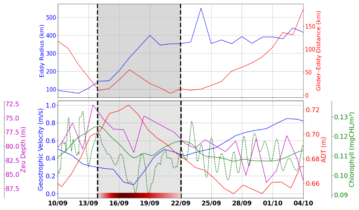
Figure 4 Top: time series of the distance between the glider and the nearest eddy contour (red) and the maximum eddy radius (blue). Bottom: geostrophic velocity magnitude along the glider's track (blue), ADT along the glider's track (red), chlorophyll a concentration along the glider's track from GlobColour (solid green), integrated chlorophyll a between surface and Zpd from glider (dashed green), and euphotic depth along the glider's track (purple). The red segment represents AE1, with shading that becomes lighter towards the edge and darker at the core.

3.1.3 Biogeochemical characteristics associated with AE1

The lowest chlorophyll values (∼ 0.11 mg m⁻³) along the glider acquisition were recorded in the eddy core, which was characterized by minimal velocities and maximum absolute dynamic topography (ADT). In contrast, higher biological activity was observed at the eddy's periphery, marked by dashed black lines on 14 and 22 September (Fig. 4), emphasizing the spatial heterogeneity induced by the eddy's circulation. This pattern was explained by the typical behavior of anticyclonic eddies, where isopycnal depression inhibited the upward flux of nutrients, thereby limiting primary productivity. The coupling between the eddy's physical dynamics and the distribution of biological parameters was highlighted by the chlorophyll a maps. During the eddy-impacted period (shaded in gray), both glider (dashed green) and satellite (solid green) chlorophyll a data show a decrease at the eddy center (16–19 September) and an increase at its edge (14 and 22 September). In addition to the smoother satellite signal, the glider data reveal short-term oscillations; these high-frequency variations, likely associated with diurnal and semidiurnal processes, are not resolved by satellite observations, although the satellite successfully captures the overall trend and order of magnitude.

3.1.4 Internal solitary waves

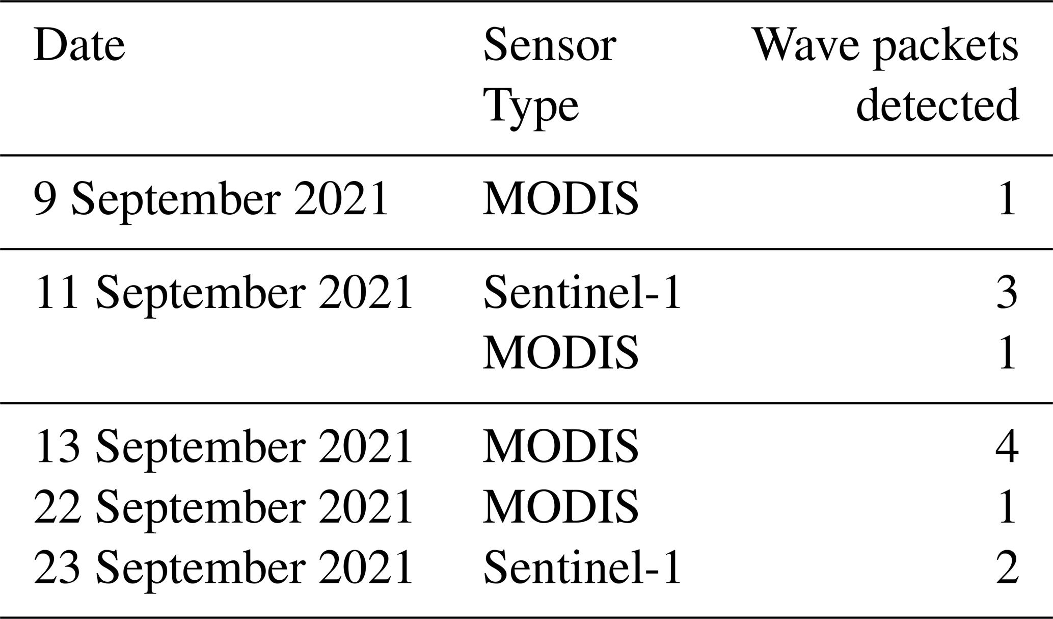
During the observation period, between 9 and 23 September 2021, a total of 12 internal solitary wave (ISW) packets were identified (Table 1). These waves were detected through a combination of satellite observation and in situ glider measurements, enabling documentation of their occurrence and dynamics over a 2-week period. Satellite images (Fig. 5a–c), acquired on 9 and 11 September (sunglint information) and on 23 September (SAR imagery), revealed the surface signatures of internal solitary waves. The glider's position, marked by an orange cross on the images, confirms the influence of intense ISWs during its evolution. Figure 5d illustrates the tidal current amplitudes derived from the FES2014 model (Lyard et al., 2021) at the point 0.5° N, 46° W. The graph highlights the variations between spring tides (blue-shaded areas) and neap tides (white areas), as well as transitional phases (yellow). The black rectangles in Fig. 5d, indicating the occurrences of solitons, show a clear alignment between the presence of internal wave trains and spring tide periods, as also shown by de Macedo et al. (2023). The observed waves primarily propagated towards the northeast, with wavelengths ranging from 117 to 175 km, characteristic of mode-1 internal waves. These structures exhibit rapid dynamics, with estimated propagation speeds of approximately 3 m s⁻¹ (de Macedo et al., 2023), significantly faster than the average speed of the glider (∼ 0.14 m s⁻¹). This speed difference explains why the glider is unable to capture the same wave crest more than once and is almost stationary in the ITs field (reduced aliasing).

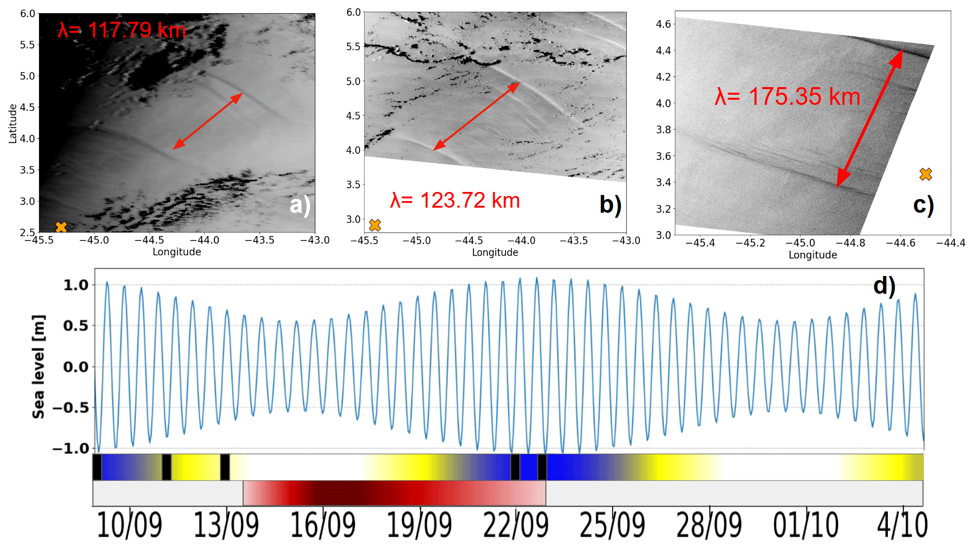
Figure 5 (a–c) Satellite imagery acquired at 13:45 UTC on 9 September 2021 and at 13:30 UTC on 11 September 2021 (both from sunglint imagery), as well as at 08:47:35 UTC on 23 September 2021 (SAR imagery). (d) Tidal current amplitudes derived from the FES2014 model (Lyard et al., 2021) at point (0.5° N, 46° W). The orange cross denotes the glider's position at the corresponding timestamps. The timeline illustrates the variation of spring tides (blue), neap tides (white), and the transient zone (yellow). The red segment represents AE1, with shading that becomes lighter towards the edge and darker at the core.

Table 1 Internal solitary waves detected by SAR (Sentinel-1) and/or Sunglint (Modis) during the period from 9 September to 5 October off the Amazon shelf and Amazon shelf break region.

3.2 Physical near-surface processes

3.2.1 Transect divided into four periods

To assess the impact of ITs on chlorophyll a, the transect was divided into distinct periods based on hydrographic criteria, ensuring a robust comparative framework. The relevance of this classification (A, B, C, and D) was validated using T/S diagrams (Fig. 7), where four distinct hydrographic profiles were identified. Period A (9–13 September, blue) was characterized by a strong salinity gradient above 23.5 kg m⁻³, ranging from 36.2 to 36.6, while temperature remained stable around 28 °C. This period was observed at edge of the NBC (Figs. 1 and 3), with a total distance of 96.69 km covered by the glider. Period B (15–19 September, red) was located within the NBC (AE1). During this phase, the glider covered a distance of 84.20 km. Period C (22–25 September, green) was identified as a transition zone between B and D, exhibiting a structure similar to period B in the 23.3–24 kg m⁻³ layer but with a saltier water mass in the 24–24.8 kg m⁻³ range. Period D (28 September to 5 October, black) was associated with waters in the influence of the North Equatorial Countercurrent (NECC) (Figs. 1, 3), where the T/S profile revealed three distinct layers within the 0–200 m column. The surface layer (23–23.3 kg m⁻³) was stratified in temperature while salinity remained constant (∼ 36.3). Beneath it, an intermediate transition layer (23.3–23.7 kg m⁻³) was marked by coherent T and S gradients, followed by a deep layer, where temperature remained stratified, and salinity was stable (∼ 36.5). This classification was found to effectively capture the hydrographic variability along the transect, providing a general frame for analyzing internal tide dynamics.

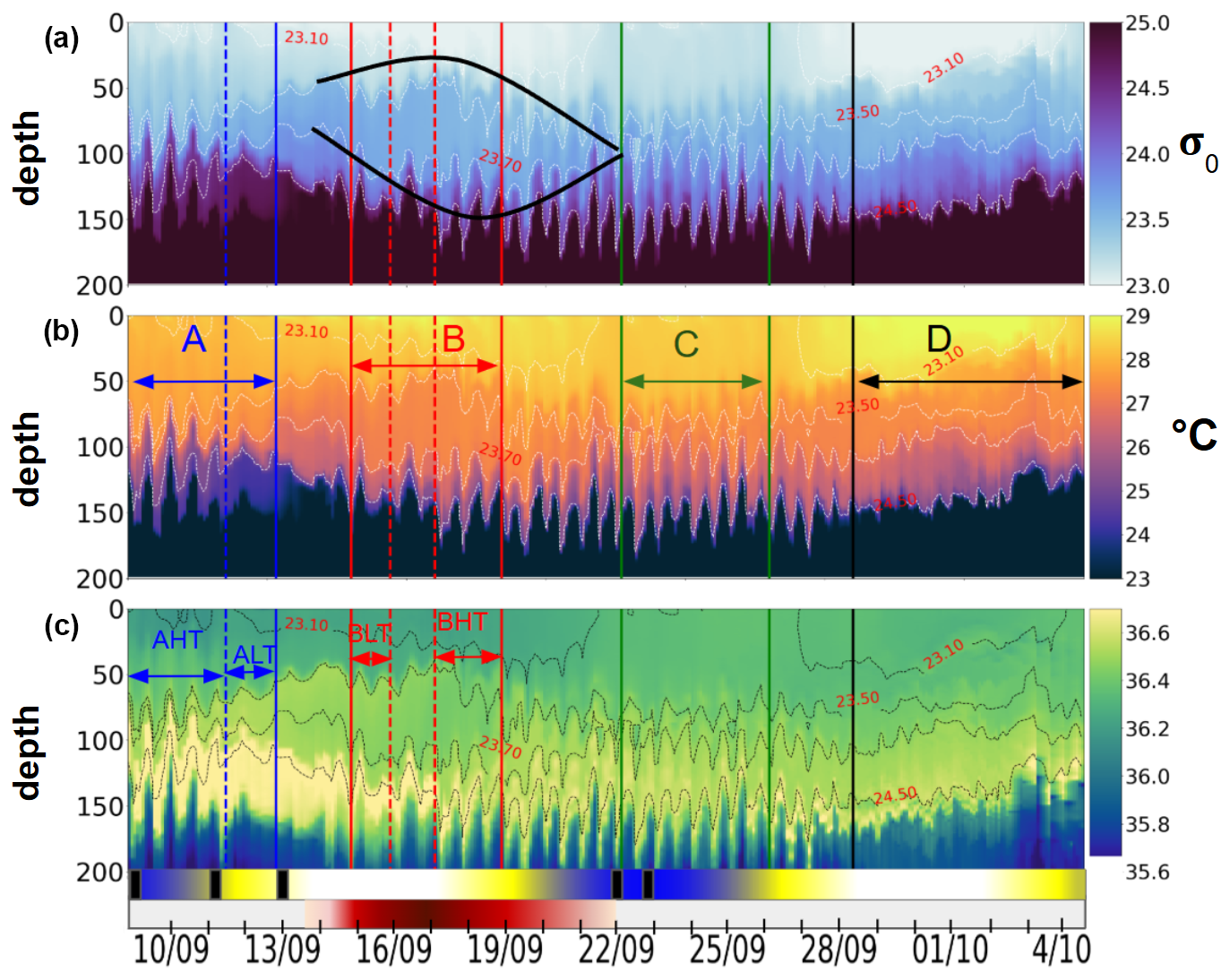
Figure 6 Hovmöller diagrams showing (a) σ₀ density (with the black lens highlighting eddy AE1 as identified in Sect. 3.1), (b) conservative temperature, and (c) absolute salinity, all derived from glider observations. The timeline below the plots indicates key oceanographic processes discussed in Sect. 3.1: blue segments mark spring tide events, white indicates neap tides, and the red segment corresponds to AE1, with shading intensity increasing from lighter at the periphery to darker at the core. A black rectangle marks the occurrence of internal solitary waves (ISWs) detected from satellite data. Labels A, B, C, and D denote distinct periods; A and B are further divided into high-tide (HT) and low-tide (LT) subperiods, reflecting variations in tidal intensity.

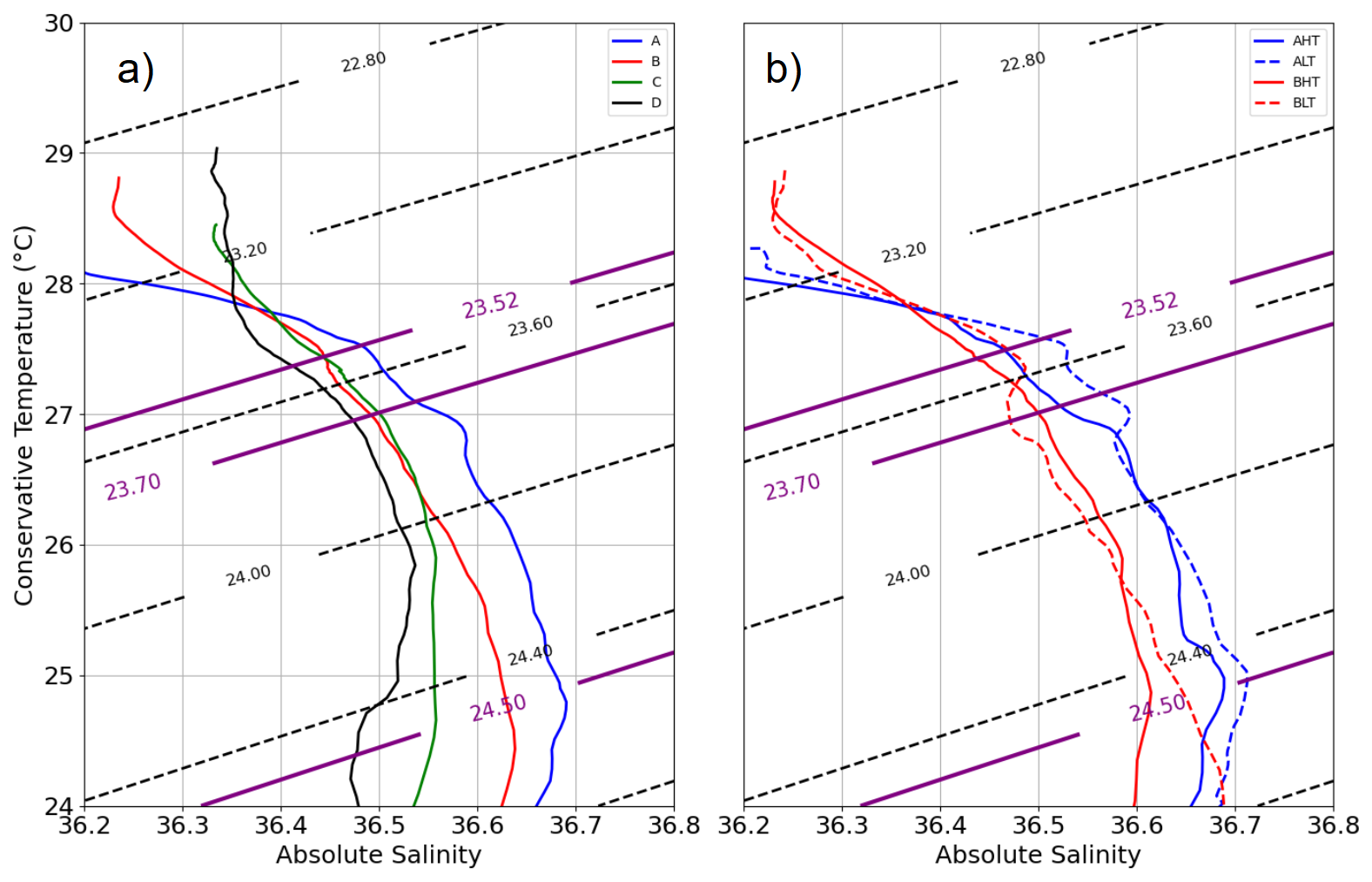
Figure 7 T/S diagram (a – left) for periods A, B, C, and D and (b – right) for the high-tide (HT) and low-tide (LT) subperiods within periods A and B. Dotted black isopycnals are plotted at intervals of 0.4 kg m⁻³.

3.2.2 Near-surface hydrography

The hydrographic observations collected by the glider between the surface and 200 m depth reveal a strongly stratified thermohaline structure, characteristic of tropical waters (Fig. 6). The temperature (T), salinity (S), and density (σ₀) profiles indicated the presence of a homogeneous layer between 0 and 50 m, followed by a thermocline, halocline, and pycnocline extending from 50 to 160 m. Salinity above 35.5 in this region indicates euhaline conditions, showing that the plume did not affect the southern area. Notable hydrographic changes are further observed during the study period. Between 14 and 22 September, as the glider crossed AE1 (marked by black lines Fig. 3a), a lenticular and homogeneous isopycnal field was detected, with nearly uniform temperature (27 °C) and salinity (36.5) between isopycnals 23.5 and 23.7 (75–125 m depth). At the surface, this anticyclone exhibited warmer and more stratified waters compared to the surrounding environment, while salinity remained homogeneous. Prior to crossing AE1, the glider was deployed at the edge of the NBC (Figs. 1, 3a) from 9 to 14 September. In contrast, this region displayed a homogeneous temperature layer but a stratified salinity profile. During this period, a maximum salinity zone (∼ 36.7) was observed between 120 and 150 m depth, generally associated with the maximum salinity transport by the North Brazil Current (NBC) (Silva et al., 2009), which was significantly reduced in subsequent periods, indicating the shift in background conditions. Between 22 and 28 September, the region was characterized by a homogeneous surface layer (0–50 m) in both temperature and salinity, accompanied by a pronounced uplift of the 23.10 isopycnal. Below 50 m, the ocean became increasingly stratified, exhibiting coherent variations in T and S. From 28 September to 4 October, the glider entered the waters of the North Equatorial Countercurrent (NECC), characterized by an accelerated geostrophic current field (Fig. 4, bottom), reaching speeds of 0.6 m s⁻¹ eastward. The hydrography during this period revealed the warmest surface layer of the transect (∼ 30 °C), followed by a coherent stratification in T and S. The four distinct regions, identified through these hydrographic variations, have been designated as A, B, C, and D, while the edges have been excluded, as they are considered transition periods.

3.2.3 Thermocline oscillations driven by ITs: variability between high and low tides

Thermocline oscillations were observed in all periods except D, with amplitudes ranging from 10 to 50 m and peaking near the 24.5 isopycnal (Fig. 6). These in-phase oscillations were most intense at the pycnocline and gradually diminished toward the surface and were modulated by neap and spring tide cycles, with peaks coinciding with internal solitary wave (ISW) events (Fig. 5). Spring tides (A and C) induced a ∼ 1 °C temperature drop, contrasting with the surface warming in period D, when no oscillations were detected. A fast Fourier transform (FFT) analysis of isotherms (145–165 m) (McInerney et al., 2019) confirms the semi-diurnal modulation of these oscillations. Periods A and B were further divided into high-tide amplitude (AHT, BHT) and low-tide amplitude (ALT, BLT) phases, while period C exhibits continuous oscillations. All showed a 12:25 spectral peak (Fig. 8) with a 10-fold increase in spectral power, confirming the influence of ITs. Furthermore, Fig. 7b reveals that these oscillatory phases correspond to the same water masses, validating the subdivision AHT/ALT and BHT/BLT.

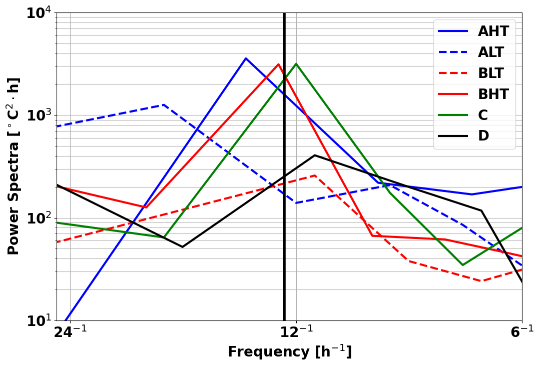
Figure 8 Spectral analysis of temperature time series in regions A, B, C, and D, across 145 and 165 m depth.

3.3 ITs effect on chlorophyll

3.3.1 Overview of subsurface processes effects on chlorophyll

The vertical distribution of chlorophyll a along the transect (Fig. 9a) was characterized by a three-layer structure. A deep chlorophyll maximum (DCM) was observed between isopycnals 23.53 and 23.7 (corresponding to depths of approximately 70 and 120 m), with concentrations ranging from 0.4 to 0.8 mg m⁻³. The lowest value (0.4 mg m⁻³) was recorded during period B, coinciding with the passage of the glider through the anticyclonic eddy AE1, in agreement with the surface signal (Fig. 4, green). At the edges of AE1, a slight uplift of the DCM was observed, attributed to the upward displacement of isopycnals. Above 23.53, a surface layer was identified, while a deeper layer extends between 23.7 and 24.5. A key finding is the influence of ITs on the vertical structure of chlorophyll a. The tides induced DCM oscillations with amplitudes between 15 and 45 m at depths of 65 to 125 m during AHT, BHT, and C, while weaker disturbances were observed during ALT and BLT (Fig. 9b). These disturbances could impact primary production, as the light gradient is non-linear – an uplift exposes the chlorophyll a layer to more light than the quantity lost by a downlift. The following section focuses on the characterization and quantification of the IT processes of advection and mixing that influence chlorophyll a distribution.

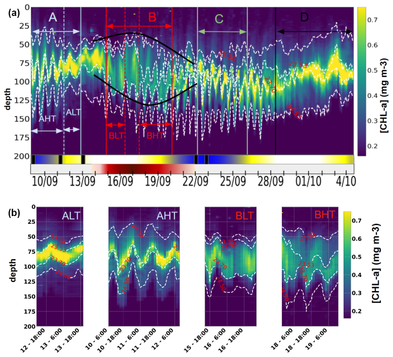
Figure 9 (a) Hovmöller diagram of chlorophyll a distribution from 0 to 200 m between 9 September and 4 October 2021. Dark green segments indicate spring tide events, while light green segments correspond to neap tides. The red segment represents anticyclonic eddy 1 (AE1), with lighter shades at the edges and a darker core. The black rectangle highlights the presence of internal solitary waves (ISWs). (b) Hovmöller diagram of chlorophyll a from 0 to 200 m, segmented by tidal phases: ALT, AHT, BLT, and BHT.

3.3.2 Variability in chlorophyll a structure between high and low ITs

Higher chlorophyll a concentrations were found at the surface and in deeper layers during HT, while chlorophyll a concentration is more pronounced within the DCM during LT (Fig. 10). To assess these variations and evaluate the impact of ITs on the vertical redistribution of chlorophyll, four key parameters were examined: maximum chlorophyll a concentration, chlorophyll a peak thickness, total averaged chlorophyll a content, and DCM depth (Table 2). The chlorophyll a peak thickness corresponds to the depth range where concentrations exceed 0.2 mg m⁻³.

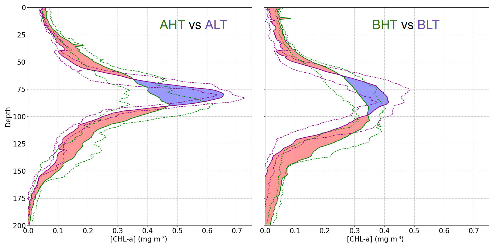
Figure 10 Comparison of mean chlorophyll a profiles during HT and LT periods. The dashed purple lines represent the interquartile range (IQR) for LT periods, while the dashed green area represents the IQR for HT periods. The red regions indicate where the mean chlorophyll a concentration during HT exceeds that during LT, and the blue regions indicate the opposite (LT > HT).

Under HT conditions, total averaged chlorophyll a content increased significantly, indicating an overall enhancement of primary production, with increases of 14 % (ΔCHL_total= 4.44 mg m⁻², where ΔCHL_total is the total variation of averaged integrated chlorophyll a between HT and LT) in period A and 29 % (ΔCHL_total= 6.98 mg m²) in period B. This increase was associated with internal tide-induced vertical displacements of chlorophyll, which redistributed biomass across different layers. Specifically, maximum chlorophyll a concentration decreased by 17 % (0.12 mg m⁻³) in period A and 9 % (0.04 mg m⁻³) in period B, while the peak thickness expanded by 50 % and 30 %, respectively. The resulting redistribution led to an inverse relationship between maximum chlorophyll a concentration and DCM thickness (Fig. 11). This correlation was statistically significant, with Pearson coefficients of r= −0.44 (p= 0.01) for period A and r= −0.29 (p= 0.04) for period B. Total averaged chlorophyll a content increased significantly during HT, with increases of 14 % (ΔCHL_total= 4.44 mg m⁻², where ΔCHL_total is the total variation of averaged integrated chlorophyll a between HT and LT) in period A and 29 %, (ΔCHL_total= 6.98 mg m²) in period B, indicating an overall enhancement of primary production.

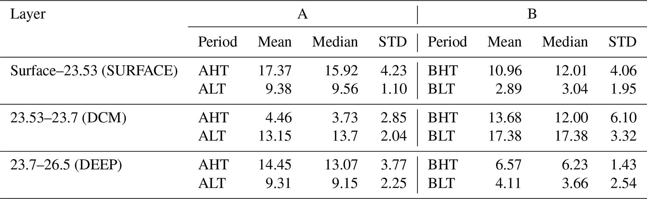
Table 2 Summary statistics of chlorophyll a of four key parameters: maximum chlorophyll a concentration, chlorophyll a peak thickness, mean chlorophyll a content, and the depth of the deep chlorophyll a maximum during HT and LT periods. “STD” stands for standard deviation.

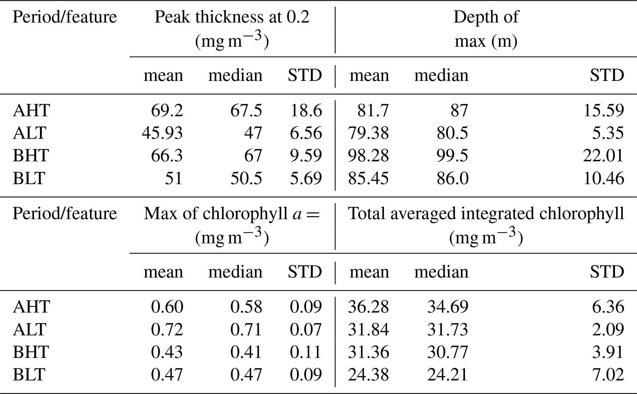
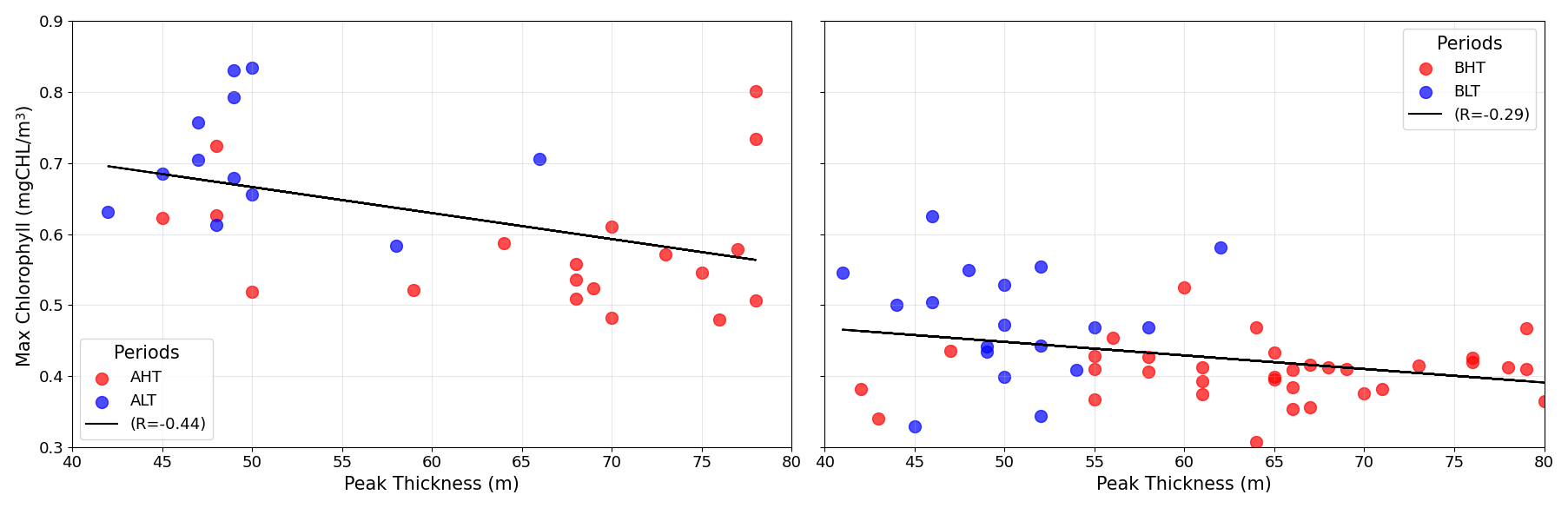
Figure 11 Relationship between chlorophyll peak thickness (m) and maximum chlorophyll a concentration (mg m⁻³) during HT and LT periods.

3.3.3 Chlorophyll a diapycnal redistribution

The net chlorophyll a loss observed in the deep chlorophyll a maximum (DCM) layer between low tide (LT) and high tide (HT) was estimated at ΔCHL_DCM= −8.69 mg m⁻² or a 64 % loss during period A (−3.7 mg m⁻² or 21 % loss during period B), as shown in Table 3. This depletion was redistributed both upward and downward across isopycnal layers.

Table 3 Diapycnal statistics of integrated chlorophyll a concentrations for each isopycnal layer.“STD” stands for standard deviation.

The downward turbulent flux reaching the deep isopycnal layer (23.7 < σ₀ < 26.5) was quantified as ΔCHL_DEEP = 5.14 mg m⁻² in period A (2.46 mg m⁻² in period B). As this layer lay below the euphotic zone and did not support photosynthesis, biological consumption processes dominate (ΔSMS_DEEP < 0), implying that the observed chlorophyll a increase represented a minimum estimate of the turbulent flux to depth ΔCHL_DEEP < =ΔDiff_DEEP (Eq. 7). Thus, turbulent fluxes from the DCM supplied approximately 57 % of the total chlorophyll a increase observed in the deep layer. The turbulent flux toward the surface layer (σ₀ < 23.53) was consequently estimated by mass conservation as ΔCHL_DCM−ΔDiff_DEEP=ΔDiff_SURF = 3.55 mg m⁻² for period A (1.09 mg m⁻² for period B). Thus, turbulent fluxes from the DCM supplied approximately 38 % of the total chlorophyll a increase observed in the surface layer. The total variation in surface chlorophyll a content between LT and HT reached 7.99 mg m⁻² in period A (8.07 mg m⁻² in period B). After accounting for the turbulent input, the contribution of biological processes (production minus grazing) was calculated at ΔSMS_surf= 4.55 mg m⁻² for period A (6.98 mg m⁻² for period B).

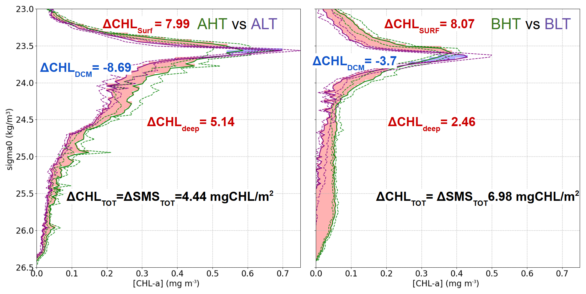
Figure 12 Average vertical profiles of chlorophyll a concentration (mg m⁻³) as a function of density (σ₀, kg m⁻³ ) for two regions: AHT vs. ALT (left) and BHT vs. BLT (right) based on density bins of 0.03. Shaded areas indicate differences in chlorophyll a concentration between regimes, with red representing positive differences and blue indicating negative differences. Dashed green and purple areas represent the first and the third quartile for HT and LT periods.

4 Discussion

4.1 AE1 as a mode-water eddy

In this study, AE1 was identified as a mode-water eddy with an isopycnal structure distinct from that of classical anticyclonic eddies. While classical anticyclonic eddies typically feature depressed isopycnals that form a bowl-like shape, restricting nutrient access to the euphotic zone, cyclonic eddies are characterized by domed isopycnals that enhance nutrient uplift. Mode-water eddies, a particular type of anticyclone, combine both doming and depression of isopycnals and have been reported as productive systems in subtropical regions (Chelton et al., 2011; McGillicuddy et al., 2007). In the case of AE1, isopycnals around σ₀ ≈ 23.5 exhibited a doming structure, whereas the isopycnal at σ₀ ≈ 23.7 displayed a bowl-shaped pattern (Fig. 6). Notably, during period B, AE1 was less productive compared to other periods, which contrasts with McGillicuddy et al. (2007) (Fig. 9). In McGillicuddy's framework, the doming part of an anticyclonic system can drive isopycnal uplift, potentially enhancing biological productivity by injecting nutrient-rich waters into the euphotic zone. In our case, while such isopycnal uplift is indeed observed within AE1, the anticyclone core appears too deep for this mechanism to significantly increase productivity, likely because of the uplift. This finding suggests that the productivity of mode-water eddies or lens-shaped eddies is strongly influenced by their depth. Consequently, the deep chlorophyll maximum (DCM) and likely the nutricline were situated deeper, limiting light availability and constraining photosynthetic activity.

4.2 Dominance of ITs over near-inertial waves

One may ask whether wind forcing contributes significantly to the observed variability. Figure 13 shows a spectral analysis of the glider data over the whole period of acquisition (1 month). A clear and intense peak is observed at 1×10⁵, close enough to the M₂ 12.25 h (Figs. 8 and 13). At the inertial period (approximately 7 d at 2–4° N), a small peak at 5×10³ is found, suggesting that the wind-driven processes like near-inertial waves are less important in our region.

Figure 13 Spectral analysis of temperature from the whole time series.

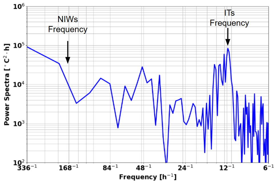
These findings support the conclusion that internal tides are the dominant oscillation that explain the intensified mixing that we estimate at the timescale of 1 month.

4.3 Limits of reversibility of LT and HT period and biological consequences

An inherent challenge with glider-based measurements is the difficulty of separating spatial from temporal variability. Because the glider moves continuously, the observed changes in hydrographic and biogeochemical properties combine true temporal evolution at a fixed location with spatial gradients encountered along the track. In our study, the definition of four hydrographically distinct regions (A, B, C, and D) was specifically designed to spatially isolate the observations. Within each region, high-tide (HT) and low-tide (LT) phases were compared under similar water mass properties, thereby minimizing the influence of large-scale spatial gradients. Averaging over multiple tidal cycles within each region further reduced short-term variability, providing a representative mean tidal signal.

Given that the deployment lasted only 26 d, our analysis primarily resolves variability on the 1–3 d timescales associated with internal tide activity, while higher-frequency (semi-diurnal, diurnal) signals are smoothed by daily averaging and lower-frequency (∼ 15 d) spring–neap modulation is only partially captured. This means that we describe only part of the total internal tide impact, focusing on its short-term expression rather than the full fortnightly cycle.

While this approach improves the robustness of our comparisons, the study remains constrained by the limited number of relevant intercomparison periods, which reduces statistical robustness and restricts our ability to generalize the observed patterns. An additional and important nuance lies in the specific sequence in which high tide (HT) and low tide (LT) occur. In the available data for period A, HT precedes LT (AHT/ALT), raising questions about the reversibility of tidal effects. The biological impact of HT followed by LT may differ significantly from a reversed sequence (ALT/AHT), particularly due to the lagged responses of phytoplankton communities. This issue is especially relevant in our study region, which is characterized by regular and intense internal tide propagation, generating near-continuous alternation between HT and LT phases. Rather than isolating the direct effect of individual ITs, our approach focuses on a comparative analysis between HT and LT conditions, acknowledging the interconnectedness and cumulative nature of these processes. Notably, the LT phase may still harbor biological communities that have benefited from favorable mixing and nutrient supply conditions during the preceding HT phase. The extent to which this occurs depends on the response time of the resident phytoplankton taxa.

In oligotrophic tropical waters such as ours, phytoplankton communities are typically dominated by small-sized cells, including Prochlorococcus, Synechococcus, and various picoeukaryotes. These groups exhibit relatively rapid physiological responses to environmental changes, particularly to nutrient enrichment. For example, Prochlorococcus can respond to pulses of nitrogen or phosphorus within 12–36 h (Moore et al., 2007; Partensky et al., 1999), while Synechococcus and picoeukaryotes tend to show measurable increases in biomass within 24–72 h (Calvo-Díaz et al., 2008; Fuchs et al., 2023; Scanlan et al., 2009; Zubkov et al., 2000). In contrast, larger phytoplankton such as diatoms are less competitive under nutrient-poor conditions and typically require more sustained or intense inputs to initiate growth, with response times ranging from 2 to 4 d (Falkowski et al., 1998; Marañón et al., 2000). In our region, assuming that the biological response occurs within approximately 1 d, this factor is unlikely to significantly influence our results. Consequently, the AHT/ALT sequence would yield similar outcomes to an ALT/AHT sequence. The cumulative evidence from our findings (Figs. 9 and 11) supports this hypothesis, suggesting that the phytoplankton species in our region exhibit a rapid response to light and nutrient availability. Further validation of this hypothesis will be achieved through complementary analysis of AMAZOMIX cytometry data in future studies.

4.4 Chlorophyll turbulent vertical fluxes

The diapycnal redistribution of chlorophyll a observed between high-tide (HT) and low-tide (LT) phases (Fig. 12) is attributed to mixing driven by internal tides (ITs), under the assumption that large-scale background conditions remain similar between HT and LT subperiods within the same overall period. Additionally, we argue that ITs dominate over near-inertial waves (NIWs) in transporting biomass both upward into the euphotic zone and downward into deeper layers. This assumption holds only if the water masses and active processes are comparable between the two phases. We verified that the water masses were sufficiently similar to support this, but we acknowledge that this approach neglects possible contributions from other vertical mixing processes, such as NIWs or frontal activity, which may differ between HT and LT. Longer time series would help quantify these fluxes more precisely, beyond the limitations of a single-event analysis.

The deep chlorophyll maximum (DCM), located at the interface between nutrient-rich deep waters and the light-limited upper layers (Ma et al., 2023), showed a net biomass loss between HT and LT, with 21 % (period B) to over 60 % (period A) exported downward and the remainder redistributed upward. These findings partly align with the observations of Gaxiola-Castro et al. (2002), who reported internal wave-driven upward transport of chlorophyll in the Gulf of California, increasing surface biomass by around 40 % during spring tides – consistent with the increases we observe. However, their study did not quantify the downward flux, which in our case accounts for nearly half of the deep-layer biomass (∼ 57 %).

This redistribution has important implications for the trophic network. As Durham and Stocker (2012) have shown, thin phytoplankton layers act as trophic hotspots, intensifying interactions among phytoplankton, zooplankton, and higher trophic levels. The downward export of biomass not only contributes to the biological carbon pump but also reduces resource availability for mesopelagic organisms. Meanwhile, the upward transfer enhances primary production, increasing surface biomass by 14 %–29 % and reinforcing upper trophic chains. Overall, these results highlight the crucial role of internal tides in shaping marine trophic dynamics and underscore the importance of accounting for both upward and downward turbulent fluxes.

5 Conclusion

This study provides new insights into the role of internal tides (ITs) in reshaping and homogenizing the vertical distribution of chlorophyll a and enhancing primary productivity off the Amazon shelf. Using a combination of satellite observations and high-resolution glider data from the AMAZOMIX 2021 campaign, we show that ITs are key drivers of short-term vertical chlorophyll variability.

The region is marked by dynamic interactions between major current systems, including the North Brazil Current (NBC), the NBC retroflection, and the North Equatorial Countercurrent (NECC), as well as the presence of mesoscale and submesoscale structures. During glider deployment, five internal solitary wave (ISW) signals and a large anticyclonic eddy (AE1) were detected by remote sensing. Combined with glider data, observations showed that AE1 locally reduced productivity by limiting exchanges between surface and deep nutrient-rich layers.

Glider profiles revealed strong vertical isopycnal oscillations between 15 and 45 m at semi-diurnal tidal frequencies. The intensity of these oscillations allowed us to separate periods of strong internal tide activity (high tide, HT) from periods of weaker activity (low tide, LT), which, under similar water mass conditions, provided a robust basis for comparing the effect of internal tides on chlorophyll a. Importantly, while ocean color satellites are unable to resolve such fine-scale diurnal variations, the glider was able to capture these dynamics, offering unique insights into the vertical redistribution of chlorophyll a.

Our results show that ITs redistribute chlorophyll a vertically. This results in a thickening of the deep chlorophyll maximum (DCM), increasing by 30 %–50 % (∼ +15 m) during high-tide periods, and a reduction in its peak chlorophyll a concentration by 9 %–17 % (∼ −0.1 mg m⁻³). These effects are the results of both the advection and mixing of the ITs.

First, the advection of the ITs induce vertical motion of the DCM, following the associated isopycnal displacement, which, when averaged, results in a larger DCM peak and, combined with light conditions, may enhance primary production since the light gradient is not linear with depth. Indeed, in the uplift condition, chlorophyll receives more light and increased primary production is expected; an uplift exposes the chlorophyll a to a greater light gain than the light loss caused by a downlift.

Second, the mixing plays a major role in reshaping the chlorophyll. Turbulent transport redistributes chlorophyll a both upward into the euphotic surface layers (accounting for ∼ 40 % of the chlorophyll content above the DCM) and downward into the aphotic deep layers (about ∼ 60 % of the chlorophyll content below the DCM), with these fluxes originating from the DCM pool and leading to losses of up to 65 %.

Overall, the combined effect of advection and mixing, by improving both light availability and nutrient supply, leads to an increase in the total chlorophyll a content integrated over the whole water column by 14 %–29 % during high internal tide phases compared to low internal tide phases.

For future research, we recommend a more systematic use of gliders in oceanographic campaigns to enhance our understanding of internal tides and their interactions with ocean biogeochemistry. We strongly advocate for the combined integration of biological, physical, and turbulence sensors to better characterize the small-scale processes that control phytoplankton dynamics and primary production.