Spatiotemporal properties of intrinsic sea level variability along the southeastern United States coastline

The influence of intrinsic ocean variability on coastal sea level remains largely unexplored but is of potential importance for emerging forecasting efforts. As in weather forecasts, intrinsic variability will amplify uncertainty in initial conditions. However, variability originating from intrinsic processes may be predictable in a forecast system with sufficient resolution and accurate initialization. Here, we examine the spatiotemporal properties of intrinsic sea level variability along the southeastern United States coast using a suite of global ocean/sea-ice simulations at 0.1° horizontal resolution. In model simulations, intrinsic variability is a dominant component of the monthly de-seasonalized and detrended sea level variability in deep waters, but it is damped along continental shelves, where it comprises ∼ 10 %–30 % of the sea level standard deviation. Our analyses demonstrate that US East Coast and Gulf of Mexico shelves exhibit a common intrinsic mode, with maximal amplitude in the South Atlantic Bight and almost no expression north of Cape Hatteras. This intrinsic coastal mode is coherent with sea level along the Gulf Stream axis after detachment from Cape Hatteras. Intrinsic sea level variability in the detached Gulf Stream leads the coastal mode by 2–3 months, suggesting that intrinsic coastal sea level variability may exhibit predictability.

1 Introduction

Coastal ecosystems, communities, and economies are highly susceptible to sea level variability over a wide range of timescales (e.g., Rashid et al., 2021; NOAA, 2022). Accurate sea level predictions are needed for mitigation and adaptation purposes and for effectively managing risks associated with sea level variability. Such predictions will benefit from (1) improved understanding of relevant drivers of regional coastal sea level variability, and (2) assessment of the representation of monthly to interannual coastal sea level variability in dynamic models utilized for operational ocean forecasting.

Various physical processes operating at different spatial and temporal scales influence sea level variability (e.g., Gerkema and Duran-Matute, 2017; Little et al., 2019; Camargo et al., 2024). These processes can be partitioned into a deterministic component that occurs in response to an applied forcing (“atmospherically forced component”), and a non-deterministic (“intrinsic”) component, which is not directly driven by atmospheric variability but is instead generated by the ocean itself, for instance, through small-scale (i.e., mesoscale and smaller) turbulent processes (e.g., Penduff et al., 2011). Such small-scale processes become particularly important in eddy-active regions of the ocean and cause the ocean's evolution to be non-deterministic at both small and large (regional to basin) scales under prescribed forcing conditions (Sérazin et al., 2015; Qiu et al., 2015; Forget and Ponte, 2015; Close et al., 2020).

Sea level variability originating from intrinsic processes might be a significant source of uncertainty in forecasts and can only be represented by adopting ocean models of sufficient horizontal resolution (e.g., Penduff et al., 2010, 2011; Sérazin et al., 2018; Chassignet et al., 2020). However, generally, the horizontal resolution of ocean models used for coastal sea level forecasts is on the order of 1° (∼ 100 km), which is insufficient to capture the effect of oceanic intrinsic variability on coastal sea level (e.g., Long et al., 2021).

Even in simulations capable of representing intrinsic processes, separation of forced and intrinsic variability is not trivial. Two strategies have been used to isolate the contribution of intrinsic variability in eddy-permitting ocean model simulations. The first strategy compares model output from a realistic atmospherically forced model with one only subjected to climatological forcing (e.g., Stewart et al., 2020) (i.e., repeat-year forcing simulations). The second approach employs ensemble members with perturbed initial conditions, which permit the estimation of the forced (ensemble mean) and intrinsic components (i.e., difference between time series of a specific member and the ensemble mean) (e.g., Penduff et al., 2014; Bessières et al., 2017; Donatelli et al., 2025).

This paper focuses on characterizing the spatiotemporal properties of intrinsic sea level variability along the southeastern coast of the United States (including the Gulf of Mexico), where societal vulnerability to sea level variability is high and increasing (e.g., Thatcher et al., 2013). The majority of the studies in this area focus on atmospherically forced variability (e.g., Frederikse et al., 2017; Calafat et al., 2018; Piecuch et al., 2018; Wang et al., 2024) and less is known about the influence of oceanic intrinsic processes on coastal sea level.

The southeastern coast of the United States (from now on, SEUS) has a strong intrinsic component at subannual to interannual timescales (e.g., Close et al., 2020; Little et al., 2024). However, previous studies do not elucidate: (i) the SEUS along-coast spatial structure, and (ii) how coastal variability relates to offshore variability over space and time. To explore these questions, it is essential to use simulations that (1) represent the SEUS shelf topography with sufficient grid points, even in regions where the shelf narrows, and (2) adequately resolve offshore intrinsic variability (e.g., Hallberg, 2013).

Here, to study the spatial structure (and magnitude) of intrinsic sea level variability along the SEUS coastline and its spatiotemporal relationship with offshore variability, we utilize monthly sea surface height (SSH) fields from high-resolution (HR) forced ocean/sea-ice (FOSI) and repeat-year-forcing (RYF) (Stewart et al., 2020) simulations performed using the Community Earth System Model at 0.1° horizontal resolution (Chang et al., 2020; Yeager et al., 2023; Little et al., 2024). We utilized the HR FOSI simulation to evaluate whether the model faithfully represents observations, and the HR RYF simulation to cleanly estimate intrinsic sea level variability. The paper is organized as follows. The model setup, observational datasets, and data processing are described in the Appendix. In Sect. 2 we show the results, and in Sect. 3 we present the discussion and conclusions.

2 Results

2.1 Total and intrinsic sea level variability

We first compare the total (i.e., forced plus intrinsic) sea level standard deviation from the HR FOSI simulation and observations over the 1993–2018 period (Fig. 1). Total sea level standard deviation (mean across the FOSI members; Fig. 1a) is larger in deep waters and decreases over the continental shelf. Over the same temporal window, a gridded altimeter product (Fig. 1b) shows a similar spatial structure, with the model generally underestimating the observed monthly total sea level standard deviation over the shelf by 10 %–20 %. A similar result was obtained when we compared coastal grid points with the detrended and de-seasonalized sea level recorded by tide gauges (TGs). At three representative locations along the US coastline (Fig. 1c, d, e), discrepancies between model and TG observations were more significant in Galveston (see standard deviations in Fig. 1c, d, e). In contrast, Charleston exhibited the largest inter-cycle differences. Our results show that, overall, sea level hindcasts compare favorably to TG observations over the 1993–2018 period (see Table 1).

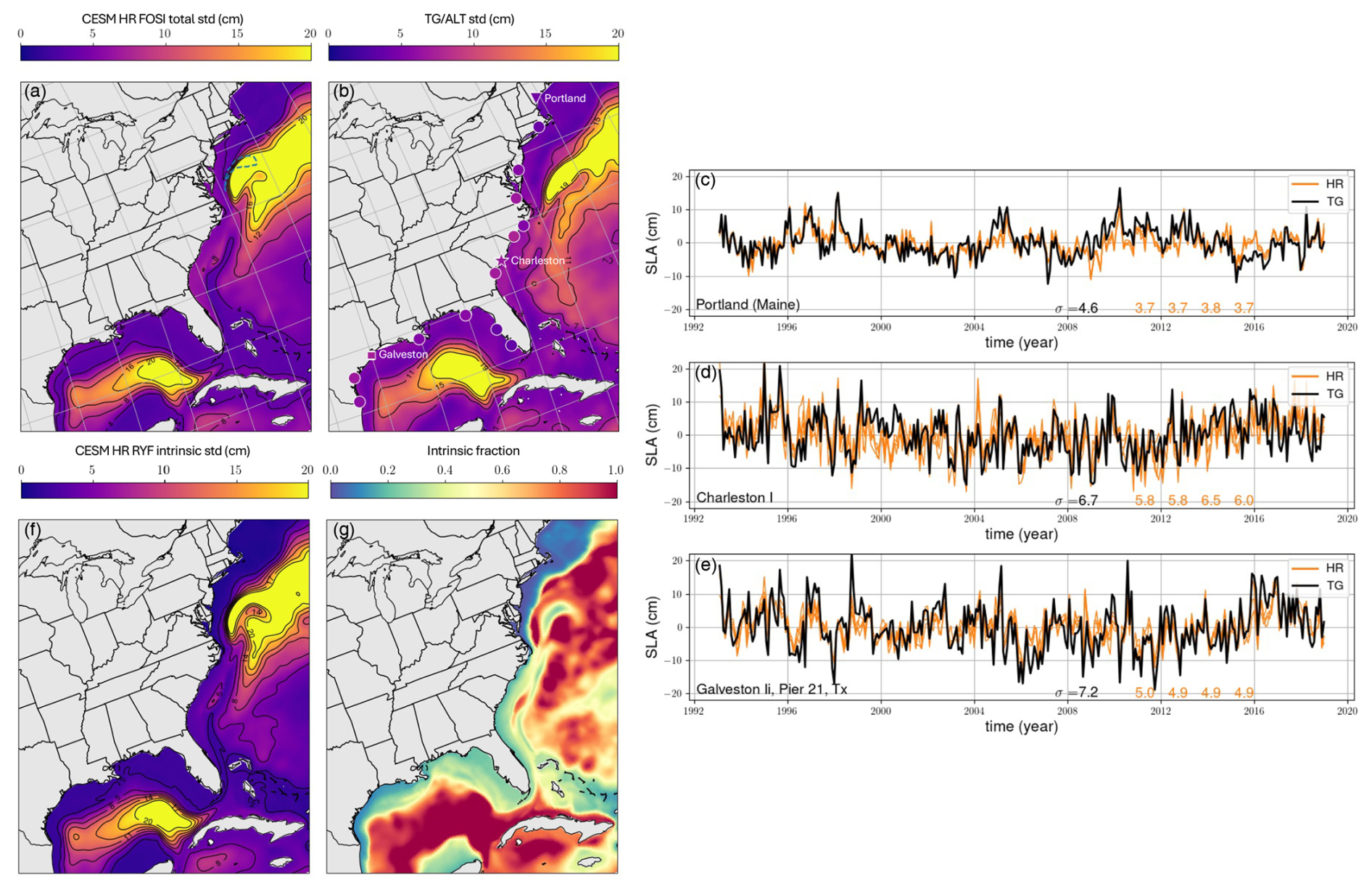
Figure 1 Total sea level standard deviation (cm) from (a) the HR FOSI simulation (the blue dashed line indicates the offshore region in Fig. 3a) and (b) gridded altimeter product over the period 1993–2015. (c, d, e) Comparison between detrended and de-seasonalized time series from tide gauges (TGs) and HR FOSI ensemble simulation in three representative locations. We reported the standard deviation (cm) for TGs (black) and each FOSI cycle. The location of each TG is shown in Fig. 1b. (f) Intrinsic standard deviation (cm) estimated using the HR RYF simulation. (g) Intrinsic fraction (i.e., intrinsic standard deviation estimated from the HR RYF simulation divided by total standard deviation computed using the HR FOSI simulation).

Table 1 Comparison between HR FOSI simulation and TG observations. For each ensemble member, we reported coefficient of determination (R²) and root mean square error (RMSE).

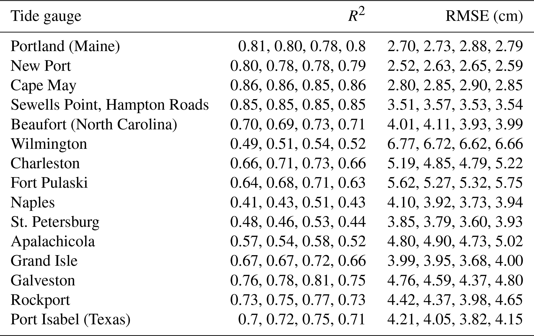
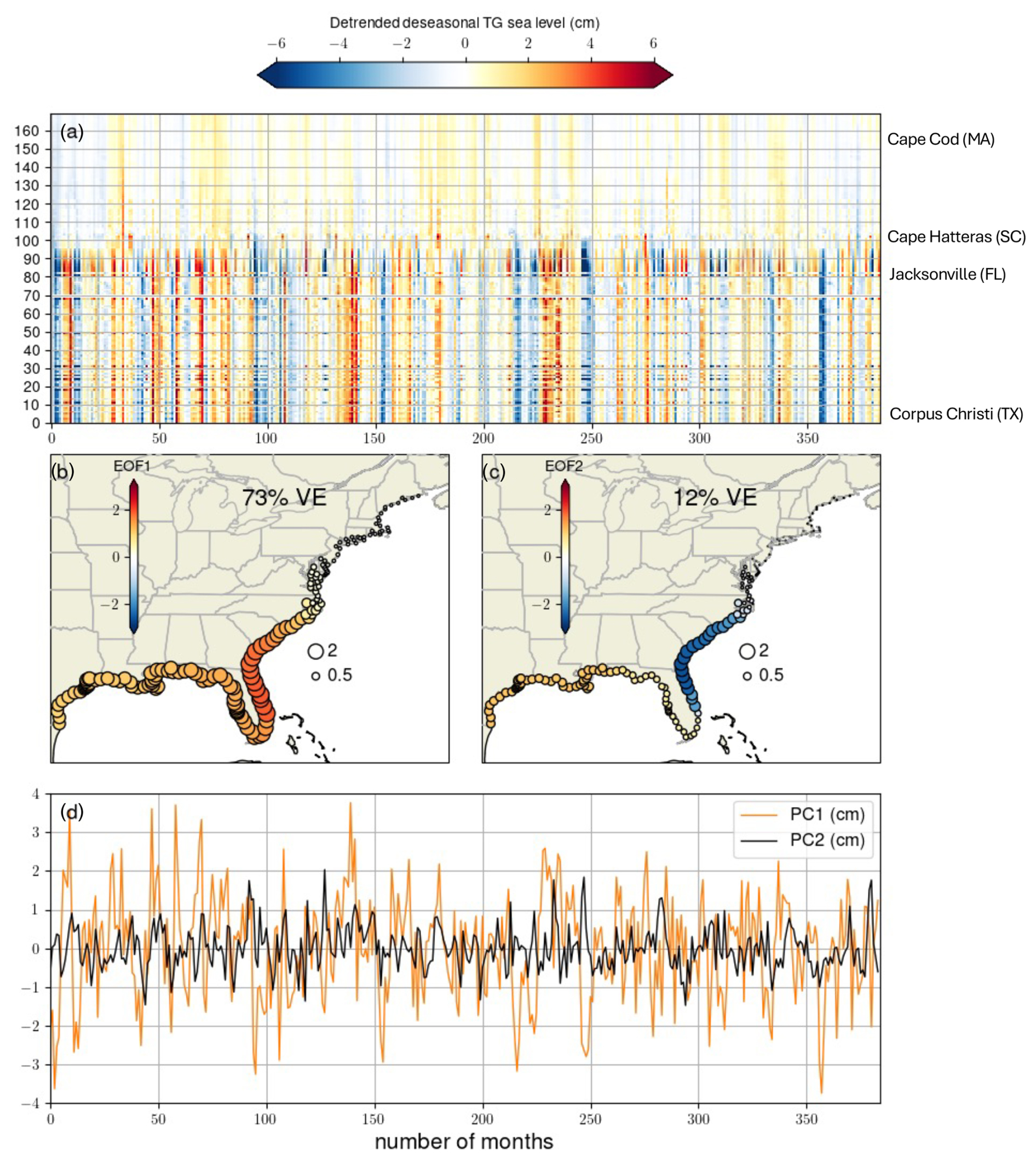
Figure 2 (a) Monthly time series from the HR RYF simulation extracted at 170 pseudo-TGs along the SEUS coastline. These time series are 32 years long. (b) First mode and (c) second mode obtained from EOF analysis. The color of the circles indicates the eigenvectors' value in each pseudo-TG, while the circles' radius is related to the magnitude. (d) Principal components (PCs, cm) associated with modes 1 and 2.

We next quantify intrinsic variability using detrended and de-seasonalized monthly outputs from the HR RYF simulation (Fig. 1f). The intrinsic standard deviation shows substantial spatial variations; specifically, it is damped on the continental shelf relative to offshore. By computing the intrinsic fraction (i.e., ratio between the intrinsic standard deviation from the HR RYF simulation and the total cycle-mean sea level standard deviation from the HR FOSI simulation), we found that the intrinsic standard deviation represents 10 %–30 % of the total sea level standard deviation on the continental shelf south of Cape Hatteras and up to 100 % of the total standard deviation in deep waters (Fig. 1g; note that these results pertain to a region dominated by a western boundary current). Offshore intrinsic variability is maximized in the interior of the Gulf of Mexico and in proximity to the Gulf Stream (GS). Along the GS path, we found a minimum in the offshore intrinsic fraction (Fig. 1g), which coincides with a region of low intrinsic standard deviation (Fig. 1f). The core of the GS is characterized by weaker zonal SSH gradients with respect to its margins (see SSH contours in Fig. 3). These spatial variations in SSH gradients may be responsible for the patterns observed in offshore intrinsic variability near the GS.

2.2 Intrinsic sea level variability along the SEUS coast

We utilized detrended and de-seasonalized monthly SSHs extracted at 170 coastal grid points (pseudo-TGs) from the HR RYF simulation to analyze the spatial structure of intrinsic sea level variability along the SEUS coast. Consistent with Fig. 1f, g, coastal grid points exhibit minimal variability north of Cape Hatters (see pseudo-TGs between locations 100 and 170 in Fig. 2a).

We used EOF analysis to identify the modes that explain the largest fraction of the variability along the SEUS coastline. The EOF decomposition revealed that the first two modes explain most of the variability in the dataset. Specifically, the first mode explains 73 % of the variability, while the second mode contributes 12 % (Fig. 2b, c). The eigenvector associated with the dominant mode showed the same sign in all the pseudo-TGs (as indicated by the color of the circles in Fig. 2b), revealing a “common mode” linking the East Coast and the Gulf of Mexico. In contrast, the second eigenvector suggests that the pseudo-TGs along the US East Coast behave opposite to those in the Gulf of Mexico (Fig. 2c). The variability explained by each mode presents significant spatial variations (see the size of the circles in Fig. 2b, c), particularly between pseudo-TGs south of Cape Hatteras (larger) and those north of Cape Hatteras (smaller standard deviation). Both modes show enhanced variability between Cape Hatteras and Jacksonville.

The temporal evolution of the first two eigenvectors is represented by the PCs associated with each mode (Fig. 2d). The PCs exhibit fluctuations at subannual to interannual timescales, including multi-year sea level trends (for example PC1, over a 5-year period beginning around month 90) (Penduff et al., 2019). The remainder of the paper considers only the first mode (PC1) given its dominant role in explaining SEUS intrinsic coastal variability.

2.3 Relationship between along-coast and offshore intrinsic sea level variability

We utilized detrended and de-seasonalized SSH fields obtained from the HR RYF simulation to identify spatial pathways connecting offshore and coastal intrinsic sea level variability. With no lag, PC1 correlates with (i) SSHs over the entire continental shelf south of Cape Hatteras, and (ii) SSHs within an off-shelf region located in proximity to the GS axis after detachment from Cape Hatteras (Fig. 3a).

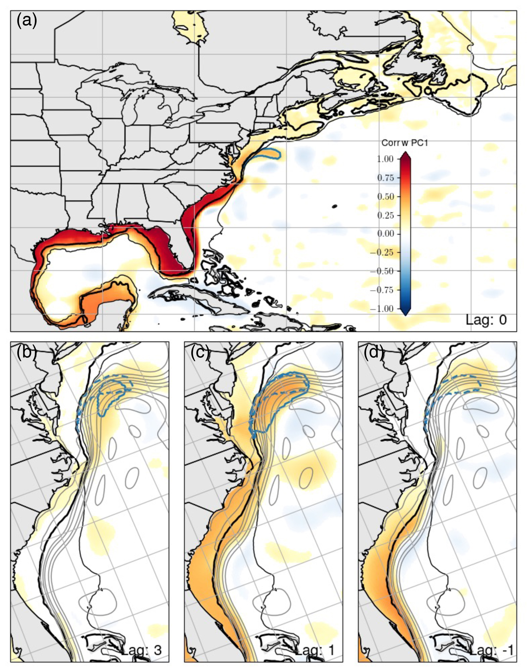
Figure 3 Lag correlations between the PC1 and SSH field: (a) no lag, (b) lag of 3 months, (c) lag of 1 month, and (d) lag of −1 month. A positive lag means that SSH field leads the PC1. The solid blue line in panel (a) shows the off-shelf region when no lag is applied to the PC1. The solid lines in panel (b), (c) represent the off-shelf region when lags of (b) 3 months and (c) 1 month are applied to the PC1. The dashed lines in panels (b), (c), and (d) show the off-shelf region when no lag is applied to the PC1 (i.e., the dashed lines are the same as the solid line in panel a). The statistical significance of the lag correlations was evaluated using a p value of 0.05. The thicker black lines indicate a water depth of 100 m, while the lighter black line indicates a water depth of 1000 m. The grey lines are time-mean SSH contours at 10 cm intervals.

To assess evidence for propagating oceanic signals, lag correlations at different lags were applied, with a positive lag indicating that offshore sea level leads PC1. We highlight correlated off-shelf regions (blue contours in Fig. 3b, c, d) using a threshold of 0.3 (note that coherence analysis performed in the following paragraph is not sensitive to the precise threshold employed to identify the detachment region). Interestingly, lag correlations reveal that the off-shelf region (i) moves westward and varies in size with decreasing time lag, and (ii) leads the along-coast intrinsic mode.

We employed a spectral approach to further characterize the relationship between the PC1 and the detrended and de-seasonalized SSHs over the off-shelf region (i.e., solid blue line in Fig. 3a). The two-time series show high coherence values (coherence amplitude greater than 0.5, Fig. 4a) for frequencies smaller than 0.9 yr⁻¹. In this frequency band, the coherence phase lag (positive phase lag denotes off-shelf region leads the PC1; shown only for frequency bands where coherence is statistically significant) ranges between 20 and 40° (i.e., off-shelf region leads PC1 by 2–3 months). To help visualize these results, we applied a 13-month low-pass filter to the two-time series (Fig. 4b). Consistent with Fig. 4a, the two filtered signals show that the off-shelf region leads the along-coast intrinsic mode.

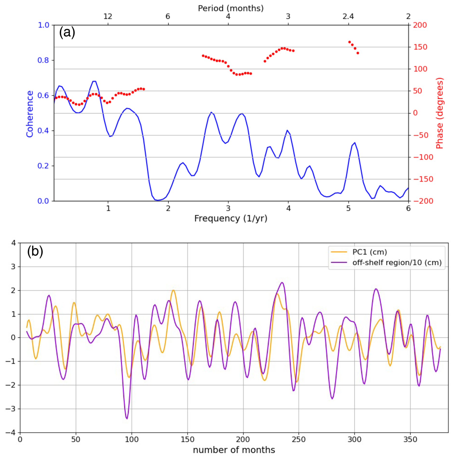
Figure 4 (a) Coherence analysis between the PC1 and average SSH signal within the off-shelf region. Note phase lag is only shown for statistically significant coherence (a positive phase means that the off-shelf region leads the PC1). (b) PC1 (cm) and average SSH signal (cm) within the off-shelf region to which we applied a 13-month low-pass filter. The average SSH signal within the off-shelf region is divided by 10.

3 Discussion and conclusions

Using a 50-member ocean ensemble hindcast at 0.25° horizontal resolution, Close et al. (2020) showed that sea level variability is almost entirely driven by intrinsic processes in energetic regions of the ocean, such as the GS. Building on this study, we utilized a set of numerical experiments at higher spatial resolution to explore the linkage between offshore and coastal sea level variability along the SEUS coastline.

Our analyses revealed that, at monthly to interannual timescales south of Cape Hatteras, intrinsic processes meaningfully contribute to sea level variability, reaching up to 30 % of the total monthly sea level standard deviation on the continental shelf. A common intrinsic sea level mode, largest between Charleston and the Florida Straits, but coherent around the Gulf of Mexico, is correlated with sea level variability in the detached GS through a large-scale pathway connecting deep and shelf waters. The absence of intrinsic variability to the north of Cape Hatteras is consistent with the limited ability of eddies to influence sea level where the shelf is wide (e.g., Gangopadhyay et al., 2020), and the equatorward propagation of coastal sea level anomalies originating near the GS detachment.

The along-coast coherence of PC1, and the robust 2–3 month lag between off-shelf and coastal sea level variability (see offshore region in Fig. 3), inform hypotheses about the underlying oceanic mechanisms controlling the propagation of sea level anomalies from the off-shelf region to the coast (e.g., Wu and He, 2025). Our results are consistent with propagation along the continental slope via topographic Rossby waves (e.g., Wise et al., 2018, 2020; Hughes et al., 2019). The latter travel with a speed of a few centimeters per second at these latitudes (first baroclinic mode), roughly consistent with the time lag we quantified between the off-shelf region and the PC1 (barotropic Rossby waves may also be involved in this transfer process). Once sea level anomalies break the potential vorticity barrier and penetrate onto the shallow continental shelf (e.g., Wise et al., 2020), they are transmitted via Kelvin waves traveling at a few meters per second (first baroclinic mode); such signals can travel from Cape Hatteras to the Gulf of Mexico in less than a month. This lag is not resolved using the monthly SSH fields available from the HR RYF and is thus consistent with our identification of a single signed coastal mode. Given the disparity between open-ocean and coastal wave speeds, daily SSH fields will be required to capture the along-coast propagation of sea level anomalies.

The frequency band in which the along-coast intrinsic mode and the off-shelf region exhibit high coherence suggests that SSH within the off-shelf region might be influenced by variations in the GS position excited by intrinsic oceanic variability (e.g., Quattrocchi et al., 2012; Grégorio et al., 2015). More specifically, frequencies smaller than 0.9 yr⁻¹ seem consistent with interannual GS path oscillations, which are known to control a significant fraction of the total SSH variance within the GS detachment region (e.g., Guo et al., 2023). Related to this point, it is important to mention that the GS is often misplaced in numerical models (Chassignet and Marshall, 2008). This GS separation bias produces excessive surface EKE north of Cape Hatteras in POP (Parallel Ocean Program, Smith et al., 2010) HR FOSI (Chassignet et al., 2020) and, therefore, we can expect that it may also impact the magnitude of the along-coast mode detected in the HR RYF simulation.

CESM simulations show that intrinsic sea level variability is smaller (in a time-aggregated sense) than forced sea level variability; however, it is not negligible and, as noted, may have inherent predictability. Although the origin of atmospherically forced and intrinsic sea level variations is different, our study reveals that the oceanic mechanisms involved in the communication of off-shelf anomalies to the coast (and from Cape Hatteras to the Gulf of Mexico) are similar to those regulating the transfer of some previously described forced sea level signals (e.g., Calafat et al., 2018; Dangendorf et al., 2021, 2023; Steinberg et al., 2024). As such, our findings help understand the role of GS path variations (forced and intrinsic) on coastal sea level, and we suggest that sea level forecasting efforts will benefit from further studies of intrinsic variability along the SEUS coastline and elsewhere. This study provides a better understanding of (i) the physical processes governing offshore-shelf and shelf-to-shelf communication along the SEUS coastline, and (ii) the relationship between offshore GS variations and coastal sea level (e.g., Ezer et al., 1995, 2013; Wu and He, 2025). It may also help with the interpretation of observational datasets (e.g., Oelsmann et al., 2024).

Appendix A: CESM simulations

We employed an HR FOSI simulation with a spatial resolution of 0.1° (∼ 10 km) to analyze monthly SSH fields from 1993 to 2018. The HR FOSI simulation represents the response of the ocean and sea ice to prescribed atmospheric forcing (e.g., wind, temperature). This simulation was performed using the global Community Earth System Model version 1.3 (CESM1.3) following the Ocean Model Intercomparison Project version 2 (OMIP2) experimental protocol (Griffies et al., 2016). The 1958–2018 forcing applied is (nearly) identical in each of four consecutive cycles (or ensemble members) and is obtained from JRA55 reanalysis. The JRA55 atmospheric fields have a spatial resolution of 55 km and a temporal resolution of 3 h. The HR FOSI simulation was initialized from observed climatology (i.e., World Ocean Atlas) and spun up through consecutive cycles of 1958–2018 (61-year) forcing. Each cycle repeats the forcing of the previous simulation (e.g., simulation years 62–122 (cycle 2) repeats the forcing of simulation years 1–61 (cycle 1)). Since the cycles share the same forcing but have different initial conditions, inter-cycle differences can be largely attributed to intrinsic processes.

The limited number of HR FOSI cycles does not allow a clear separation of forced and intrinsic variability (although estimation of the forced and intrinsic variance might be possible using inter-cycle differences, see Little et al., 2024). To cleanly quantify intrinsic variability, we use an HR RYF (repeat-year forcing) simulation. The HR RYF simulation was carried out by applying a single year of JRA55 boundary conditions from May 2003 to the end of April 2004. The May 2003–April 2004 year is characterized by low (non-anomalous) values for major climate modes. The May–April cycle is to avoid forcing discontinuities in mid-winter. By applying the same annual forcing in each year, interannual variability in sea level can be mainly attributed to oceanic intrinsic processes. Here, we analyzed the last 32 years of monthly outputs from a 70-year-long HR RYF simulation to examine the spatiotemporal properties of intrinsic sea level variability along the SEUS coastline, over the continental shelf, and adjacent deep waters. The HR RYF simulation was selected because of its unprecedentedly high resolution (0.1°), which allows us to examine the linkage between offshore and along-coast intrinsic sea level variability. Further details of the model setup can be found in Little et al. (2024).

Appendix B: Observational dataset and comparisons with model outputs

We utilized monthly mean TG observations with less than 12 missing months over the 1993–2018 period. TG observations were obtained from the Permanent Service for Mean Sea Level Revised Local Reference database on 1 December 2022 (Holgate et al., 2013). Missing data were infilled using linear interpolation after removing the seasonal cycle from the time series.

Sea level recorded by TGs is affected by numerous processes not accounted for in CESM simulations (e.g., inverted barometer effect, barystatic changes, global mean steric expansion/contraction, and vertical land motion). Thus, we removed from the TG record (i) the inverted barometer effect, using surface pressure fields from the ERA-5 atmospheric reanalysis, and (ii) the global mean sea level due to barystatic and steric processes, employing estimates obtained from altimetry (MEaSUREs, 2021). Additionally, we linearly detrended the corrected TG time series to account for vertical land motion (after correction and detrending, we denote sea level as ζ^′).

To compare model output and sea level observed by TGs, we extracted the SSH in the closest model grid points to each TG using a ball tree algorithm (i.e., a ball tree algorithm is an efficient means of finding model grid points closest to a list of TG locations; more details can be found at https://scikit-learn.org/stable/modules/neighbors.html (last access: 1 March 2025). The modelled time series were detrended to remove model drift. To evaluate the model performance at larger spatial scales, we compared the spatial structure of ζ^′ variability from the HR FOSI simulation with a $\mathrm{1}/\mathrm{6}$° gridded satellite altimeter product at monthly temporal resolution over the 1993–2018 period (MEaSUREs, 2022). Before comparing the two datasets, we removed the global mean sea level and linearly detrended the residual at each grid point from the altimeter product (note that the inverted barometer effect has already been removed from the altimeter gridded product).

Appendix C: Additional data processing

SSH time series were extracted from the HR RYF simulation along the SEUS coast at 170 pseudo-TGs (one pseudo-TG for each model grid cell along the coast). Then, we applied empirical orthogonal function (EOF) analysis to the extracted SSH time series to identify the modes that explain the largest fraction of variability in the dataset. First, a matrix (O) was created by storing the time series extracted from the HR RYF simulation along each column. Then, we computed the covariance matrix (C=O^TO) and solved the corresponding eigenvalue problem:

$$\begin{array}{}\text{(C1)}& \mathbf{C}=V\mathit{\lambda }{V}^T,\end{array}$$

where V and λ are the eigenvector and eigenvalue matrices. Each eigenvalue indicates the fraction of the variance explained by each eigenvector. By expressing matrix O in the space identified by the eigenvectors, we computed the principal components (PCs) associated with each mode.

We also utilized coherence analysis to characterize the relationship between along-coast and offshore intrinsic sea level variability. The spectrum was obtained by applying a Hanning window with overlapping (50 % overlap) data segments. Each data segment has a length of 64 time steps (i.e., 64 months) and starts halfway through the previous segment (i.e., each data segment captures half of the data of the previous one). Coherence uncertainties were obtained using a standard approach (e.g., Gallet and Julien, 2011). This approach sets a threshold to assess whether a computed coherence exceeds what might be expected from random noise. The threshold is determined based on the significance level (i.e., 95 % significance level) and the number of segments used to compute the coherence spectrum. The number of segments was evaluated as the time series length divided by the window length multiplied by 0.5.