Application of quality-controlled sea level height observation at the central East China Sea: Assessment of sea level rise

This study presents a state-of-the-art quality control (QC) process for the sea level height (SLH) time series observed at the Ieodo Ocean Research Station (I-ORS) in the central East China Sea, a unique in situ measurement taken in the open sea for over 2 decades at a 10 min interval. The newly developed QC procedure, named Temporally And Locally Optimized Detection (TALOD), has two notable differences in characteristics from the typical ones: (1) spatiotemporally optimized local range check based on the high-resolution tidal prediction model TPXO9 and (2) consideration of the occurrence rate of a stuck value over a specific period. In addition, the TALOD adopts an extreme event flag (EEF) system to provide SLH characteristics during extreme weather. A comparison with the typical QC process, satellite altimetry, and reanalysis products demonstrated that the TALOD method could provide reliable SLH time series with few misclassifications. A budget analysis suggested that the sea level rise at the I-ORS was primarily caused by the barystatic effect, and the trend differences between observations, satellite, and physical processes were related to vertical land motion. It was confirmed that ground subsidence of −0.89 ± 0.47 mm yr⁻¹ is occurring at I-ORS. As a representative of the East China Sea, this qualified SLH time series makes dynamics research possible spanning from a few hours of nonlinear waves to a decadal trend, along with simultaneously observed environmental variables from the air–sea monitoring system at the research station. This TALOD QC method is designed to process SLH observations in the open ocean, but it can be generally applied to SLH data from tidal gauge stations in the coastal regions.

1 Introduction

Sea level height (SLH) comprises both oceanic components such as tides and currents, and atmospheric components (Pirooznia et al., 2016). Global warming, driven by the increased greenhouse gases, has led to a persistent increase in heat fluxes into the ocean, accelerating the rise in the upper ocean heat content and the loss of land-based glaciers and ice sheets, resulting in rapid sea level rise (SLR; Pugh et al., 2019; Fox-Kemper et al., 2021). This rise is not spatially homogeneous but localized in association with a change in the current system (e.g., Roemmich et al., 2007; Hamlington et al., 2020; Lee et al., 2022; Li et al., 2024). Rising sea levels have induced coastal erosion and broad flooding, suggesting a presumable vulnerability of populated low-lying coastal regions to global warming (Kulp and Strauss, 2019). Recent research has demonstrated a robust relationship between SLR and extreme weather events (Cayan et al., 2008; Yin et al., 2020; Calafat et al., 2022), underscoring the need for a long-term SLH monitoring network.

A global network of tidal gauges in coastal regions, along with satellite altimetry for the open ocean, has made it possible to observe worldwide sea level changes (e.g., Dieng et al., 2017; Chen et al., 2017; Cazenave et al., 2018; Royston et al., 2020; Cha et al., 2023). The upward trend of global mean SLR increased from 3.05 mm yr⁻¹ for the period 1993−2018 to 3.59 mm yr⁻¹ from 2006 to 2018, about twice faster than the 1.7 mm yr⁻¹ during the 20th century (Nerem et al., 2018; Fox-Kemper et al., 2021). The projected future sea level trend is expected to be 4.63 ± 1.1 mm yr⁻¹ for the period 2010–2060, based on observed and reconstructed measurements around Korea (Kim and Kim, 2017), implying more frequent occurrences of extreme weather and climate hazards associated with steep sea level rise in the near future.

Due to the broad socioeconomic implications of SLR, the Korea Hydrographic and Oceanographic Agency (KHOA) has constructed a sea level monitoring network comprising 38 tide gauge stations for the coastal region around Korea (red pentagram in Fig. 1). In addition, the ocean research stations, steel-framed tower-type research facilities, started to conduct continuous and autonomous observations to cover the north–south section of the Yellow and East China seas, allowing us to understand air–sea interaction and atmospheric and oceanic processes on various timescales in the open ocean (Kim et al., 2017; Ha et al., 2019; Kim et al., 2019, 2022, 2023a, b; Saranya et al., 2024). The Ieodo Ocean Research Station (I-ORS), the first one constructed at 32.125° N, 125.18° E (see Fig. 1 for its location), was established in 2003. It has been taking sea level measurements using a radar-type sensor with a 10 min interval since October 2003. This station is strategically positioned along the pathway of typhoons that impact the Korean Peninsula; hence, the I-ORS can serve as a crucial platform for comprehending extreme weather phenomena (Moon et al., 2010; Kim et al., 2017; Park et al., 2019; Yang et al., 2022) and long-term climate variability (Kim et al., 2023a).

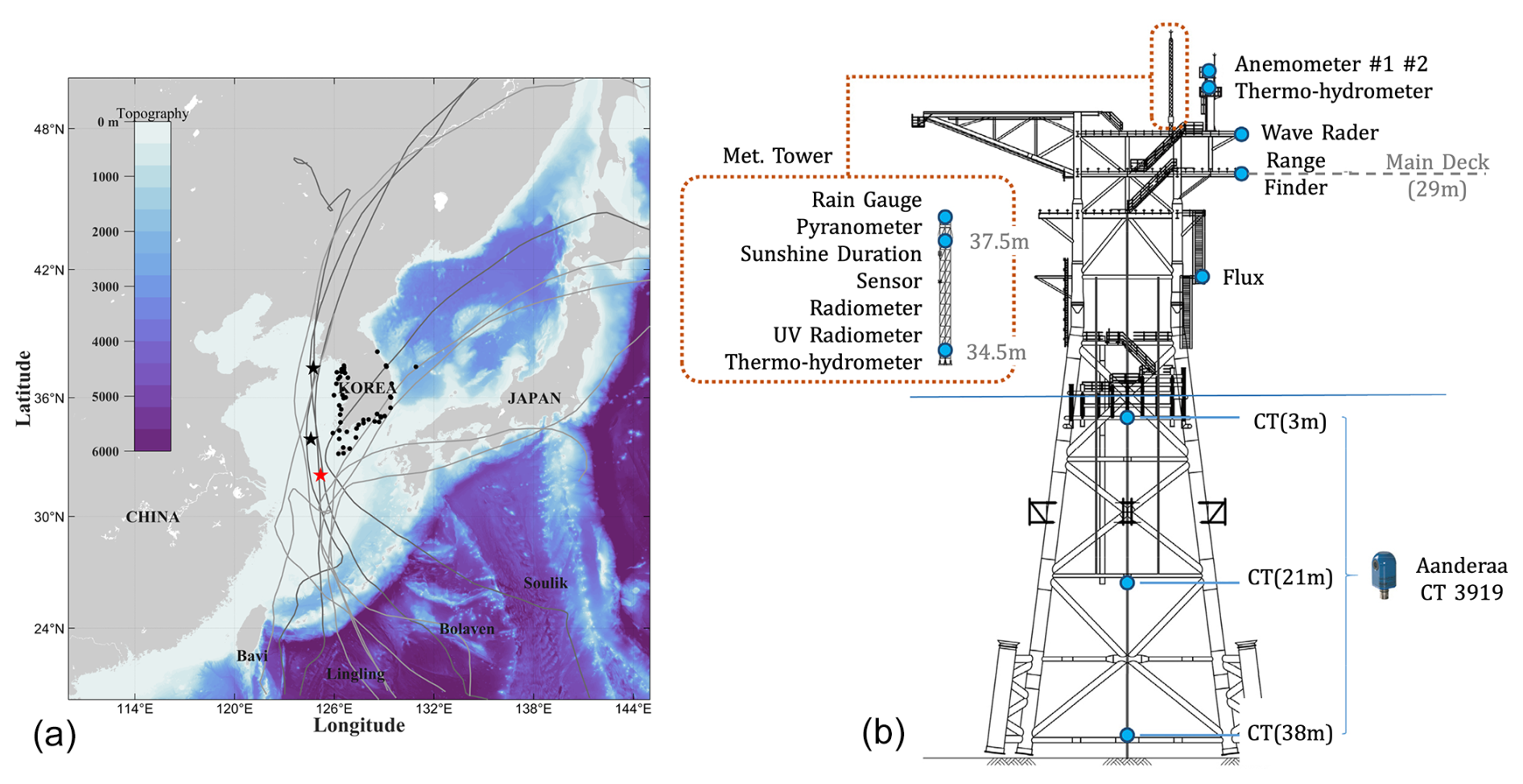
Figure 1 (a)The tracks of typhoons that passed by I-ORS (data from Joint Typhoon Warning Center; cases depicted in Fig. 6) and (b) the structure of I-ORS and instruments and the horizontal distribution for the bathymetry. The star marks indicate the location of the I-ORS (red) and the Socheongcho (black, north) and Gageocho (black, south) ocean research stations. The black dots depict the locations of tide stations. The solid gray lines show the storm tracks passing by I-ORS from 2003 to 2022 (Table 2). The darker lines indicate the typhoon case in Fig. 6.

The collected sea level data, however, contain intricate outliers such as missing data, spikes, electric noise, stucks, drift, systematic conversion (or offset)¹, and so on (Pytharouli et al., 2018). These outliers must be identified or corrected before being used for research. This process, known as Quality Control (QC), involves outlier classification into range, variability (or gradient), and sensor test categories (OOI, 2013; Min et al., 2020). Each institution utilizes a different algorithm. For instance, outliers might be identified by applying a threshold of 3 times the standard deviation above and below the average of measurements within a specified sliding window (Min et al., 2020, 2021). This approach assumes a Gaussian distribution of the observed time series; hence, it may not be suitable for uniformly applying this method because nonlinear waves or abrupt extreme events tend to be misclassified as outliers. In addition, the variables that are greatly affected by strong tides may have difficulty detecting outliers when a range check is performed without considering tidal components. Therefore, Pugh (1996) suggested a QC procedure based on tidal components estimated by a harmonic analysis. Pirooznia et al. (2019) computed tides by adopting the classical least squares (CLS) and total least squares (TLS) from raw data that contained outliers and missing values. They used the estimated tidal components to get residual components of SLH data and then performed outlier detection. Recently, Lin-Ye et al. (2023) expanded the existing SEa LEvel NEar-real-time (SELENE) QC software by incorporating additional modules to enable delayed-mode QC. In particular, the harmonic analysis-based de-tiding module was upgraded to remove tidal components. The resulting time series has been effectively utilized to identify subtle anomalies such as spikes, attenuation, and datum shifts by eliminating the periodic tidal variability from the original observations. This harmonic analysis-based approach is appropriate for the data stably obtained from tide gauge stations but seems impertinent to measurements in the open ocean, which may have various types of intricate outliers.

Previous studies attempted to verify the factors contributing to sea level rise (SLR) using various data. Cha et al. (2023) quantified and assessed the underlying processes contributing to sea level rise in the Northwestern Pacific (NWP) using reanalysis data and satellite measurements from 1993 to 2017. They found that the major contributions to SLR include land ice melt and sterodynamic (STERO) components, while the spatial pattern and interannual variability are dominated by the STERO effect. However, satellite-based sea level observations cannot detect vertical land motion such as subsidence or uplift, which may lead to trend differences between satellite and station observation. This indicates the need to analyze the variability in vertical land motion at these stations as well.

This paper aims to introduce a unique, invaluable SLH time series obtained in the open ocean over 2 decades, processed with a newly developed QC process named the Temporally And Locally Optimized Detection (TALOD) method. For this purpose, we took advantage of simulated tidal components based on the TOPEX/Poseidon global tidal model v9 (TPXO9; Egbert and Erofeeva, 2018). This high-resolution global tidal model accurately reproduces tidal components around the Korean Peninsula (Lee et al., 2022) and, hence, can be used for a local and temporal range check. The performance of the newly suggested QC process was assessed by comparing it to the KHOA method, which is based on the Intergovernmental Oceanographic Commission (IOC) Manual, and the qualified daily and monthly averaged sea level time series are assessed using satellite altimetry and reanalysed products from GLORYS12, ORAS5, and HYCOM regarding their long-term trends. Additionally, the physical processes contributing to SLR at the I-ORS were analyzed using reanalyzed products, and the vertical land motion at the I-ORS platform was estimated using the Global Navigation Satellite System (GNSS).

2 Data and methods

2.1 Observed SLH time series from the I-ORS

We constructed the TALOD QC process based on TPXO9 and applied it to the 10 min interval real-time SLH measurements obtained from the I-ORS, a total of 1 011 584 data points from 8 October 2003 to 31 December 2022. The data were measured using a MIROS SM-140 non-directional wave radar (MIROS AS, Asker, Norway), installed on the main deck 29 m above the sea surface (Fig. 1). The rangefinder principally estimates the distance to the sea surface using the reflected signals by detecting backscattered microwaves from the surface. Table 1 describes the detailed specifications of the SM-140. Sensor measurements are known to be relatively free from atmospheric conditions such as rain, fog, and water spray.

As mentioned in the introduction, the sea level measuring standard was changed on 12 December 2007. A sharp offset of approximately 6.7 m, therefore, was recorded between the data before and after the transition point (TP) (Fig. 2). Before the TP, the rangefinder recorded the distance from the sensor to the sea surface as sea level. The KHOA then altered the standard to record the actual sea level by subtracting the measured distance from the known height of the sea floor to the sensor (KHOA, 2013). Therefore, in this study, the forepart was corrected by inverting it and then adjusting it by 1.57 m to the position extrapolated to the first time of the data afterwards. In addition, we performed a harmonic analysis with the corrected SLH time series to validate the correction method. The corrected SLH time series for December 2007 estimated a sufficiently high signal-to-noise ratio (SNR) of over 10.0 (Pawlowicz et al., 2002) compared to the much broader ranges like years or decades of SLH at the I-ORS. Its amplitude and phase consistency with the rear subset also guarantees that the method corrects for the systematic offset.

Table 1 Instrument specifications for the MIROS SM-140.

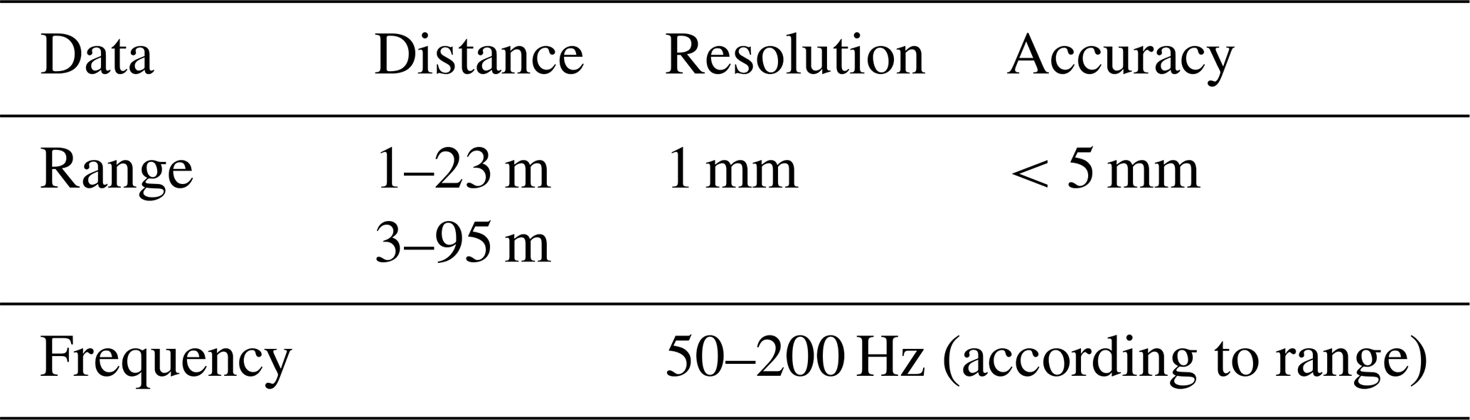
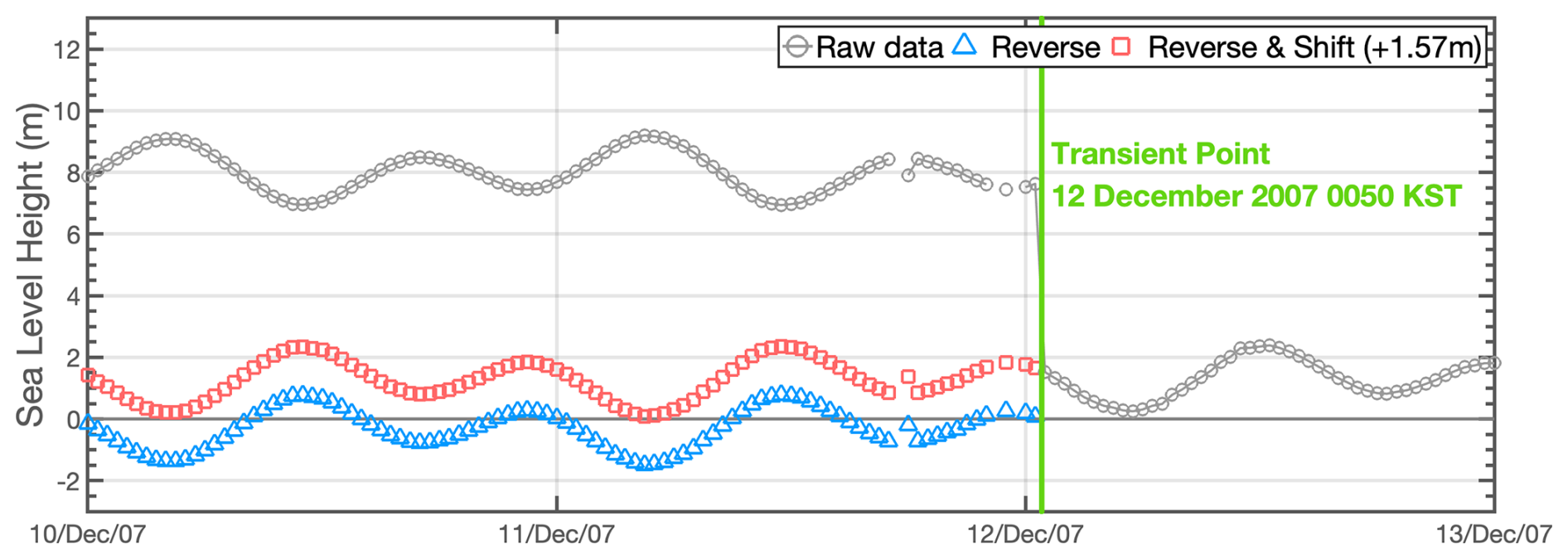
Figure 2 The circle markers indicate each process of methodological adjustment for the data before TP. The gray line with circles refers to the raw data, and the lines with blue triangles and red squares indicate the reverse and shift (+1.57 m after reversed) process.

Satellite altimetry and reanalysis products

We collected satellite altimetry and reanalysis datasets to validate the performance of the qualified SLH. The satellite data were from a gridded L4 sea surface height dataset provided by the Copernicus Marine Environment Monitoring Service (CMEMS, https://doi.org/10.48670/moi-00145, E.U. CMEMS, 2024) for 1993–2022. This altimetry, sea surface height from the geoid, was calculated through optimal interpolation (OI) by merging along-track altimetry from all satellites. Inverted barometric and tidal height corrections were applied to adjust the along-track data. The daily gridded satellite altimetry has a $\mathrm{1}/\mathrm{4}$° resolution for the global ocean. We used the daily sea surface height (SSH) time series at the grid point nearest to the I-ORS.

The three SSH products used in this study are the HYbrid Coordinate Ocean Model (HYCOM, https://www.hycom.org/, last access: 3 April 2024) data-assimilative reanalysis (HYCOM-R) for the period of 2003–2017 and HYCOM non-assimilative simulation (HYCOM-S) from 2018 to 2022, Global Ocean Physics Reanalysis 12 version 1 (hereafter GLORYS; Jean-Michel et al., 2021), and the Ocean Reanalysis System 5 (hereafter ORAS5; Zuo et al., 2019). The HYCOM product provided by the US Navy's operational Altimeter Processing System (ALPS) has a spatial resolution of $\mathrm{1}/\mathrm{12}$° by $\mathrm{1}/\mathrm{12}$° for the global ocean and a temporal resolution of 3 h. GLORYS12 was produced by Mercator Ocean International (https://www.mercator-ocean.fr/en/, last access: 3 April 2024) and has a spatial resolution of $\mathrm{1}/\mathrm{12}$° by $\mathrm{1}/\mathrm{12}$° for the global ocean with a daily resolution. The ORAS5, provided by the European Centre for Medium-Range Weather Forecasts (ECMWF), has a spatial resolution of $\mathrm{1}/\mathrm{4}$° by $\mathrm{1}/\mathrm{4}$° for the global ocean and a monthly temporal resolution (https://doi.org/10.24381/cds.67e8eeb7, Copernicus Climate Change Service, 2021). To efficiently compare sea level variability, the SLH of all datasets were converted to sea level anomalies by subtracting their mean values. Except for ORAS5, which contained monthly data, the other sea level data were averaged daily. Similarly, we estimated the daily mean observed time series when more than half of the data were available or flagged as good data.

2.2 TALOD QC

2.2.1 Manual check

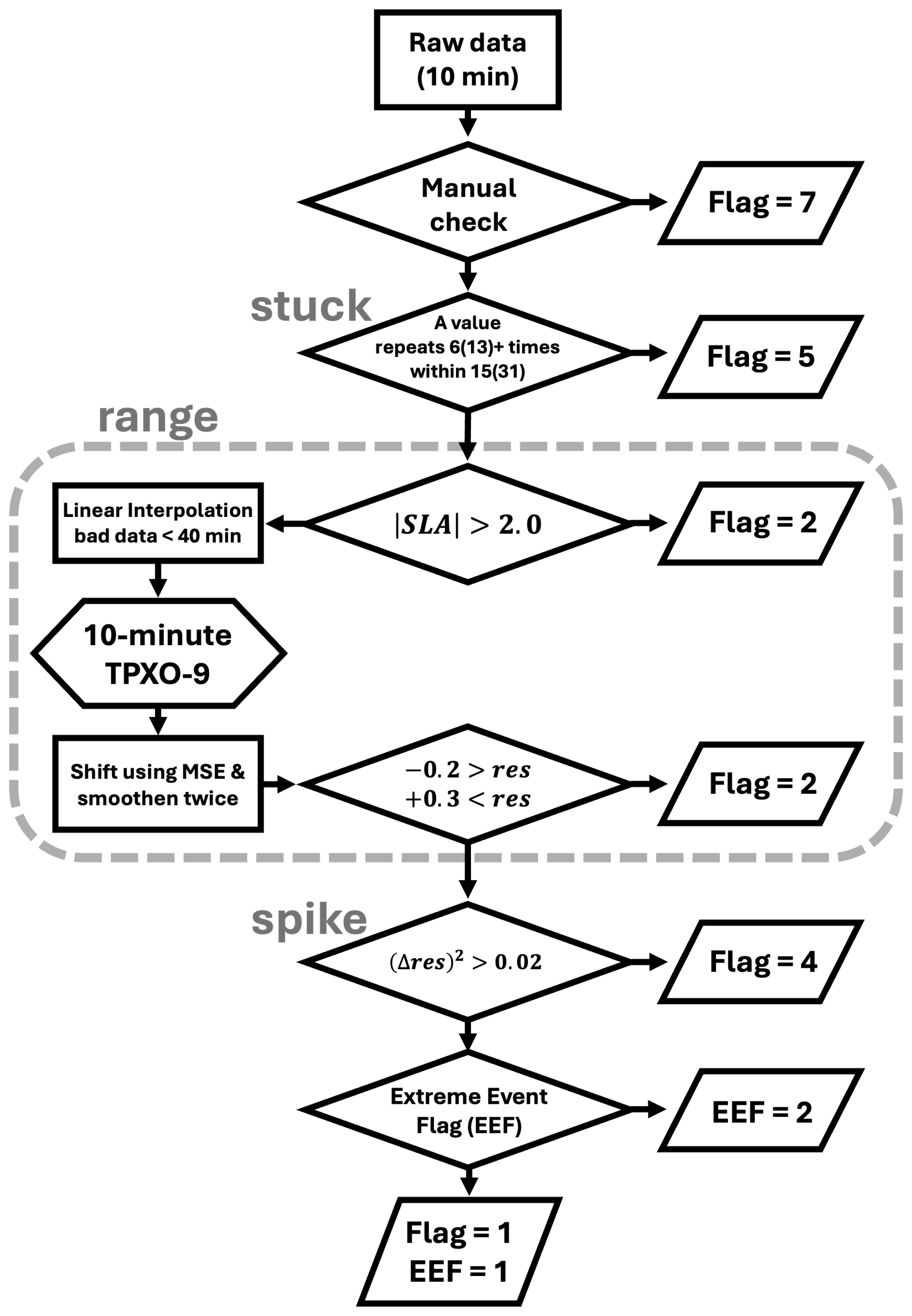
After correcting for the systematic offset in the observed sea level time series, we classified the outliers into four categories: manual, range, spike, and stuck (see Fig. 3 for a flowchart). Based on their understanding of the subsequent QC process, human operators subjectively flag data sections in the manual check – particularly those lasting more than 24 h – that may disrupt automatic detection procedures. This examination should be based on historical metadata information (or field notes) on the sensor's maintenance, cleansing, power shortage events of the station, etc. Unfortunately, metadata information concerning the observed SLH time series from the I-ORS was not made publicly available as documentation. Instead, considering the following processes, we subjectively flagged sections where the periodicity of the SLH data was irregular or nonsensical data existed for several days. For example, from June 2016 to July 2017, the sea level observations at the I-ORS involved two relocations and one replacement of the observational instrument, and the sea levels observed during this period were relatively low (not shown). As a result, 56 024 data points were flagged based on the manual check accounting for 6.32 % of the total observations. This study emphasises the significance of recorded metadata information in ensuring the quality assessment of observed time series and facilitating efficient instrumental maintenance.

Figure 3 Flow chart of TALOD QC process.

2.2.2 Stuck check

After the manual check, we recommend examining stuck values in the time series. Generally, a stuck check detects outliers when a fixed value is recorded continuously over a certain period. At the I-ORS, the SLH measurements exhibited two distinct characteristics of stuck values. First, these values persist for a certain duration without variation; typical QC processes can identify this type of stuck. Second, an abnormal case was observed at the I-ORS: alternation between normal observations (good data) and fixed values. To handle both usual and unusual stuck cases efficiently, we adopted a density of identical values over a certain period through testing various combinations of ranges and frequencies; consequently, we flagged the cases in which a single value was detected more than 6 times within a range of 15 or more than 13 times within a range of 31.

2.2.3 Range check

Typically, the range check can be divided into two parts. A local or gross range check designates a single value that is unlikely to occur naturally for a target variable at a specific location during a monitoring span. A seasonally varying range check effectively detects errors for variables dominated by seasonal variability, such as air or sea surface temperature or humidity. However, these methods are not suitable for SLH measurements in shallow water with large tidal amplitudes, such as the maximum tidal amplitude of 2.5 m that can occur at the I-ORS and significant seasonal cycles (Lee et al., 2006).

This study's range check consists of two procedures. The first is a gross range check with a fixed range, assigning upper (+2.0 m) and lower (−2.0 m) limits for the sea level anomaly (SLA). The second is a localized check with temporally varying ranges by taking advantage of the tidal prediction model. The gross range check effectively flags abnormally high values such as 29.0 and 7.98 m, which are frequently recorded in the SLH measurements from the I-ORS, even under normal weather conditions. For the local range check, we used the TPXO9 tidal model, which has a horizontal resolution of $\mathrm{1}/\mathrm{30}$°. This global tide model seems to provide accurate tidal predictions in both space and time around the Korean Peninsula, exhibiting the smallest root mean square difference (RMSD) when compared to tide gauge observations (Lee et al., 2022).

The monthly tidal data, consisting of 15 constituents (M2, S2, N2, K2, 2N2, K1, O1, P1, Q1, Mf, Mm, M4, MN4, MS4, and S1), were extracted from the TPXO9 and adjusted using the observed SLH for the same period (Fig. 4). Harmonic analysis of the observed SLH at the I-ORS shows that the M2 tide has the largest amplitude of 0.62 m. It is followed by S2 (0.32 m), K1 (0.20 m), N2 (0.16 m), and O1 (0.15 m). The mean amplitude of these primary constituents is 0.28 m, which is notably higher than that of the remaining 31 constituents with amplitudes under 0.1 m.

A monthly window is selected to consider the seasonal evolution. The extracted tidal time series was shifted to positions that minimized the root mean square errors (RMSEs), as indicated by the olive line in Fig. 4. Overshooting tends to occur when only arithmetic mean is used for the shifting, especially in convex-up and convex-down patterns, which correspond to high and low tides, respectively. This may lead to the detection of overestimated outliers. To mitigate this overshooting issue, the residual time series, i.e., the observations minus mean-shifted tides, was smoothed twice and added back to the estimated tidal time series, as shown in the salmon pink line in Fig. 4. When the difference between the observed SLH and the bias-corrected tide exceeds +0.3 m or falls below −0.2 m, the local range check identifies the data points as outliers (see Fig. 5b). These thresholds are adequate for elevation changes associated with nonlinear internal waves in this region (Lee et al., 2006).

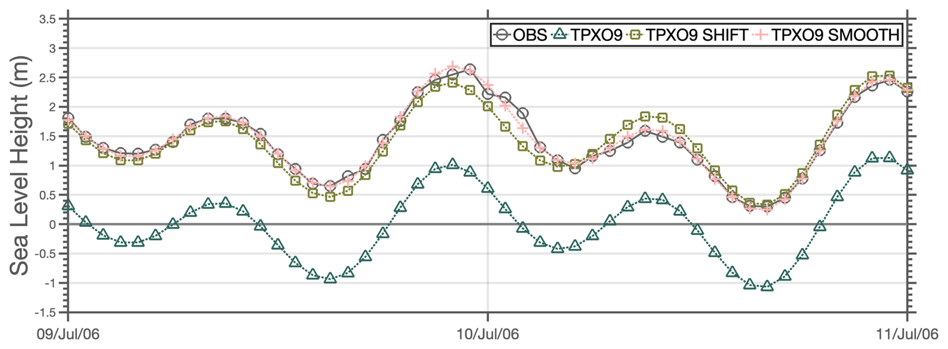
Figure 4 Lines indicate the processes for fitting TPXO9 to the observation (black line with circle) in the range check. (1) The bluish green line with triangles refers to raw TPXO9 data. (2) The olive line with squares shows mean-shifted TPXO9 based on the mean square error method. (3) The salmon pink line with crosses indicates the final output with a twice-smoothed bias added.

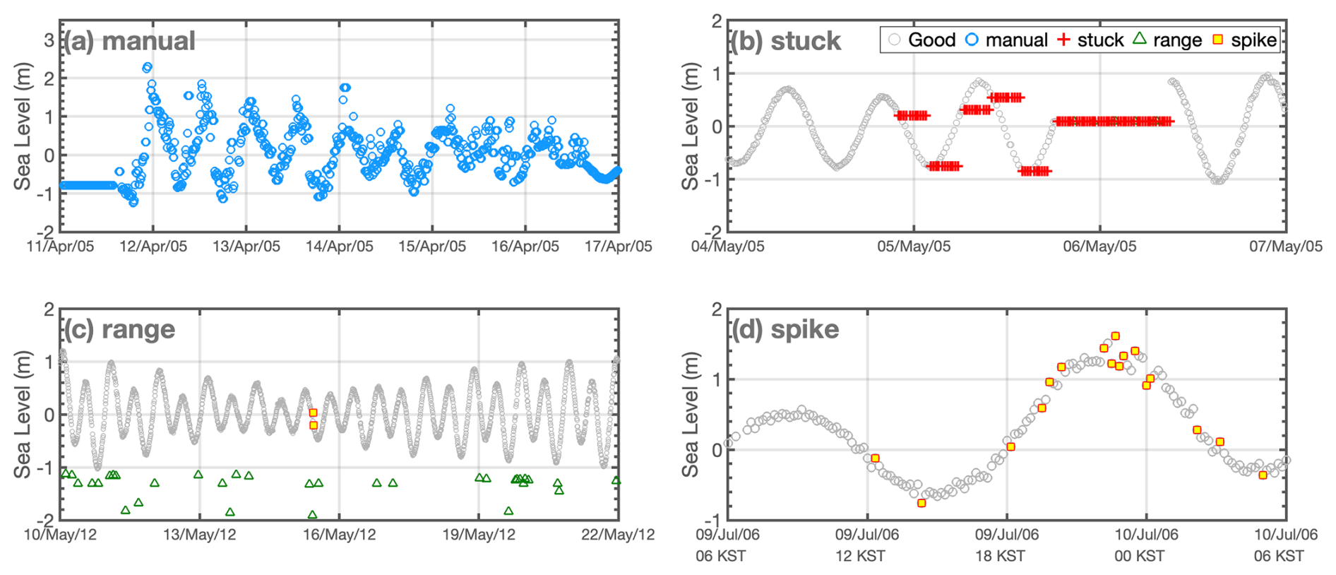
Figure 5 Time series for the examples of four flags. (a) Manual, (b) stuck, (c) range, and (d) spike. Each marker indicates good data (gray circles), manual (blue circles), range (green triangles), spike (yellow squares with red outline), and stuck (red crosses), respectively. Time series of the non-tidal residual component corresponding to Fig. 5 is provided in the Supplement (Fig. S1 in the Supplement).

2.2.4 Spike check

The spike check was developed based on the gradient spike method (GSM), following the approach of Hwang et al. (2022). The GSM typically identifies outliers by evaluating the gradient of the SLH data. However, in this study, we utilized temporal discrepancies in the non-tidal residual SLH time series. Specifically, a data point is classified as a spike if the square of its gradient exceeds 0.02. The equation used is as follows:

$$\begin{array}{}\text{(1)}& \mathrm{flag}=\mathrm{find}\left({\left(\mathrm{\Delta }\mathrm{residual}\right)}^{\mathrm{2}}>\mathrm{0.02}\right).\end{array}$$

2.2.5 Extreme event flag

Atmospheric factors such as sea level pressure and wind modulate SLH; the inverted barometer effect (IBE) and strong winds can generate abrupt fluctuations in SHL. Under extreme weather conditions, SLH measurements may be classified as outliers through range and spike checks. However, the data flagged during severe weather events may be reliable, depending on the situation. As a final QC procedure, this study introduced the extreme event flag (EEF) to provide users with an option to utilize the data based on their scientific objectives. The typhoon cases analyzed in this study are summarized in Table 2.

The observed range of SSH anomalies was nearly identical under both normal and typhoon situations, i.e., 0.30/−0.20 and 0.29/−0.20 m, respectively. However, the variance differed markedly, indicating substantial fluctuations in the SLH measurements. The variance during normal conditions was 9.0 cm², whereas it increased to 40 cm² during the typhoon-affected period, approximately a 5-fold rise. As a result, although the maximum and minimum ranges of the residual components remained almost unchanged during typhoons, the outliers classified by the spikes increased significantly (Fig. 6). We manually flagged the typhoon periods with the EEF based on the daily variance and typhoon reports issued by the Korea Meteorological Administration (KMA).

Table 2 List of typhoons during observation.

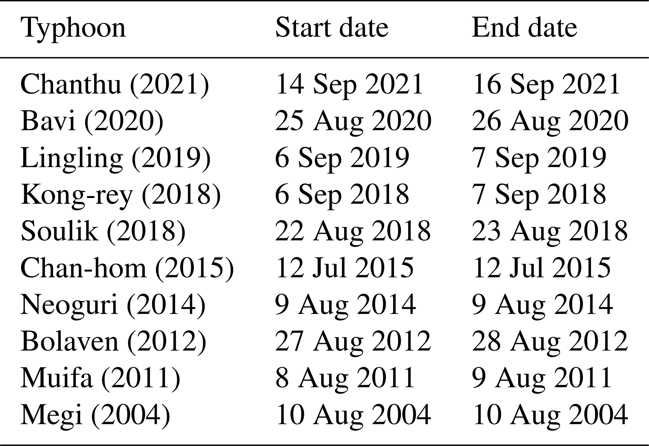
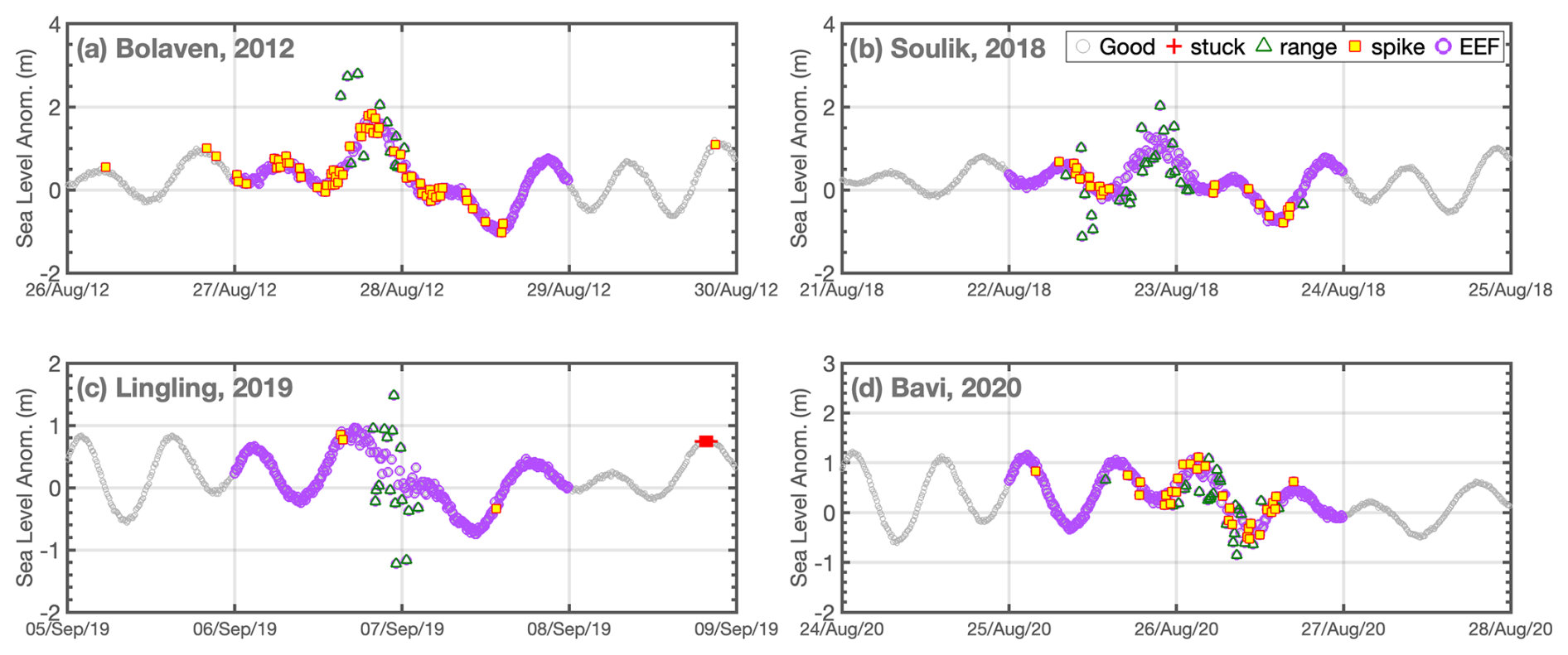
Figure 6 Time series of sea level anomalies for typhoon cases. (a) Bolaven in 2012, (b) Soulik in 2018, (c) Lingling in 2019, and (d) Bavi in 2020. Good data (gray circles), EEF (purple circles), range (green triangles), and spike (yellow squares with red outline), respectively. Time series of the non-tidal residual component corresponding to Fig. 6 is provided in the Supplement (Fig. S2).

3 Results

3.1 Comparison to existing QC process

Representative results obtained from the TALOD QC process are shown in Fig. 7, and the number and proportion of outliers flagged by each QC procedure are presented in Table 3. The results were compared with those obtained by applying the KHOA QC procedure, which follows the IOC manuals (IOC, 1990, 1993) and the NOAA handbook (NOAA, 2009), to evaluate the performance of the TALOD QC. The differences between these two QC processes are illustrated in Fig. 8 and summarized in Table 4.

Figure 7 Representative results from 1 to 15 April 2012.

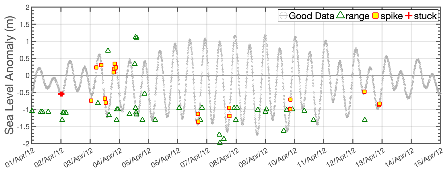
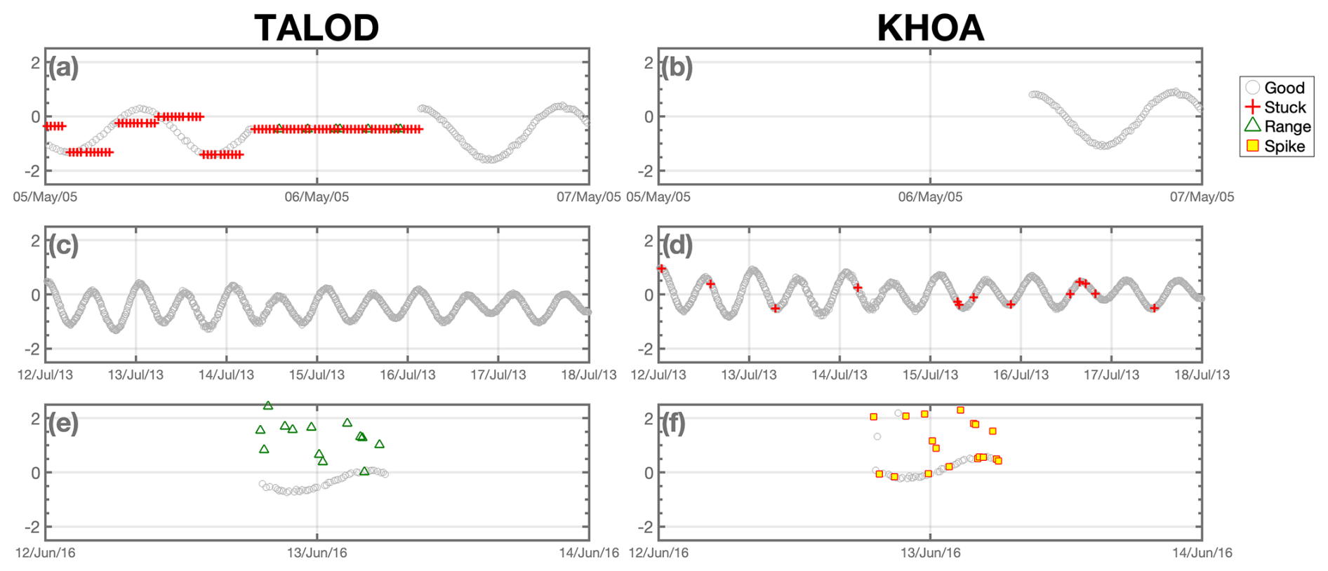
Figure 8 Same as Fig. 5 but for invariant stuck case (a–b, from 5 to 7 May 2005), stuck case during short-period (c–d, from 12 to 18 July 2013), and range–spike misclassification case (e–f, from 12 to 14 June 2016). The figures on the left and right sides show results for TALOD and KHOA, respectively. For illustrative purposes, only the flags generated by the automatic QC process were considered in (f). Comparison results with SELENE are provided in the Supplement (Fig. S3).

Table 3 Detection counts and proportions for each flag from October 2003 to December 2022 (excluding NaN values).

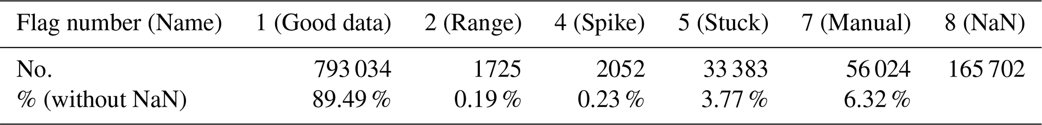
A total of 1 011 584 SLH data points were collected from the I-ORS during the observation period from 2003 to 2022. After excluding 165 702 instances with missing values (NaNs), 886 128 data points remained for quality control and analysis. Of these, 793 034 (89.49 %) were classified as good data, whereas 93 184 data points (10.51 %) were flagged as bad through the TALOD QC procedure (Table 3). Among the flagged data, excluding those flagged through the manual check, stuck values constituted the majority, representing 89.84 % of the bad data. This was followed by the spike and range flags, which accounted for 5.52 % and 4.64 % of the bad data, respectively.

Seasonal patterns in the frequency of each flag were further analyzed. The number of bad data occurrences was highest in spring, exceeding the annual average by a factor of 1.28. This seasonal increase was primarily driven by the higher incidence rate of stuck errors. Specifically, a total of 33 383 stuck errors were recorded, of which 16 536 occurred in spring – the highest among all seasons (winter: 5795; summer: 7985; autumn: 3067). The frequency of stuck errors in spring was approximately twice the annual average, presumably reflecting the influence of surface-drifting plankton on the rangefinder's reflection rate during the spring bloom period.

Other types of bad data, such as those flagged for range and spike errors, exhibited relatively low frequencies throughout the seasons, with total counts of 1725 and 2052, respectively. In contrast, manually flagged data, which represented the largest proportion of bad data, were evenly distributed throughout the year, with 56 024 occurrences (winter: 14 934; spring: 12 298; summer: 14 843; autumn: 13 949). Consequently, from a long-term perspective, the manual flag did not contribute significantly to the observed seasonal variation.

Overshooting-like errors flagged under the range and spikes categories showed peak occurrence rates during summer. This seasonal pattern coincides with the typhoon season over the Northwestern Pacific, indicating a link between extreme weather events and the occurrence of such errors.

SLH is dominated by neap-spring tidal cycles, which can lead to misclassifications in error detection when using a range check with a constant threshold. In contrast, the TALOD method employs residual components that account for rapid increases and decreases in SLH caused by diurnal tidal components and short-duration weather systems, thereby reducing detection errors. For example, the range check in the TALOD QC process successfully flagged 1936 data points as outliers. Specifically, the gross range check identified 1121 bad data, whereas the temporal and local outlier detection flagged an additional 815, efficiently capturing error-like values. The TALOD QC process preemptively flags anomalous values that severely disrupt continuity through the range checks. This approach, as illustrated in Fig. 8f, prevents detection failures caused by recurrent spike-like errors. In contrast, the KHOA's spike check has trouble with flagging spike-type errors that occur within a short time span. These unqualified outliers can degrade the performance of the spike algorithms that rely on min/max-based threshold calculations. Attention should be paid when applying the KHOA QC processes to such sea level measurements, as its automatic QC may be vulnerable to repeatedly recorded spike-like errors. For instance, among the 261 observations logged from 1 June 2016 00:00 KST to 14 June 2016 00:00 KST, the TALOD method flagged 43 instances as bad data, whereas the KHOA method identified only 37, leaving apparent error-like data unflagged (see Fig. 8e, f).

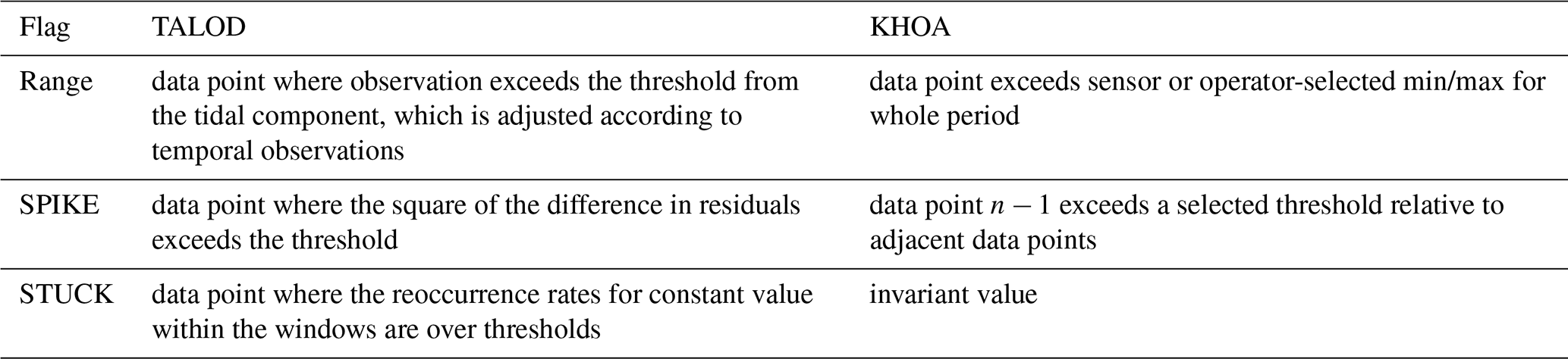
Moreover, as summarized in Table 4, the two QC processes showed remarkable differences in handling the stuck checks. While the TALOD QC process successfully detected stuck values, as illustrated in Fig. 8a, c, e, the KHOA method failed to identify these error-like values. Instead of flagging the abnormal stuck values, the KHOA QC removed the entire data segments (Fig. 8b, d, f). Furthermore, the KHOA's stuck check, which is designed to identify values as stuck when the sensor records the same values, tends to misclassify normal observations as stuck errors due to instrumental limitations including low frequency (10 min interval). Such misclassifications are frequently observed during high and neap tides (Fig. 8d). Figure S3 presents additional comparative results using the SELENE method proposed by Lin-Ye et al. (2023). SELENE failed to detect stuck errors in which NaN values alternated repeatedly with specific fixed values (Fig. S3c). Moreover, in the range and spike checks, it tended to misclassify or fail to detect errors when two or more overshooting values occurred consecutively (Fig. S3i).

Table 4 Differences in flag detection methods between TALOD and KHOA.

During the application of the KHOA process to SLH data, misclassifications or detection failures were confirmed due to the inability to identify irregularly recurring stuck errors. In contrast, the TALOD method applies optimized detection techniques and successfully flagged 45 850 stuck errors. Figure 9 shows the distribution of the observed and qualified SLAs. Compared with the idealized normal distribution (indicated by the gray line in Fig. 9), unusually high frequencies were concentrated in the ranges of −1.4 to −1.3, −0.2 to −0.1, and 0.4 to 0.5 m. After applying the TALOD QC, this distribution aligned more closely with the normal distribution, indirectly suggesting the effectiveness of the TALOD QC to identify outliers. The KHOA QC, meanwhile, appears to flag an excessive quantity of data as outliers, resulting in a distribution that deviates significantly from normality (see dark gray distribution in Fig. 9).

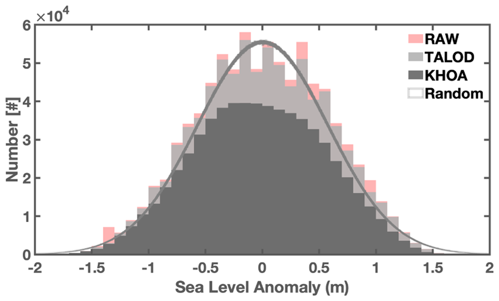
Figure 9 Histogram of observed sea level anomalies without QC (light red), with QC (light gray), and QCed by KHOA method (dark gray) from 2003 to 2022 at the I-ORS. The area enclosed by a darker gray line indicates the normal distribution.

3.2 Data validation by using observation data

Figure 10 presents the daily time series of the SLA for each dataset except ORAS5. SLH generally represents the vertically integrated heat content of the ocean; thus, higher (lower) SLAs were observed during the boreal summer (winter) period, June–September (December–March). The daily mean sea level range was approximately ±0.6 m for the observed data, −0.4 to +0.6 m for the HYCOM product, and ±0.3 m for GLORYS and satellite altimetry. We calculated the standard deviation (SD) and variance of each dataset. The SD and variance for the I-ORS measurements were 0.16 and 0.02 m, respectively; for satellite altimetry and GLORYS, the values were identical at 0.10 and 0.01 m; for HYCOM-R, 0.11 and 0.01 m, respectively. While satellite altimetry and reanalysis datasets exhibited lower SLH variability than that of in situ observations, they captured the overall pattern well, showing high accuracy with low RMSEs (less than 0.1 m). Notably, distinct differences were observed in the HYCOM dataset after 2018. Accordingly, we divided the HYCOM dataset into two periods for further analysis: before 2018 (HYCOM-R) and after 2018 (HYCOM-S).

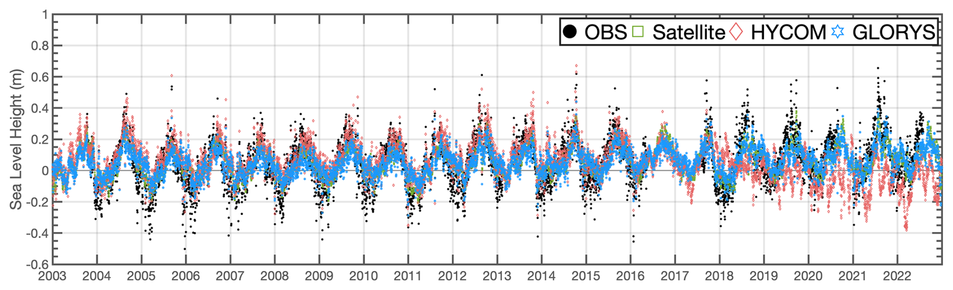
Figure 10 Time series of daily mean sea level data after QC (black dots), satellite altimetry (empty green squares), HYCOM (light red diamonds), and GlORYS12 (light cyan hexagrams) data during the observation period at the I-ORS.

First, we compared a SLR trend of each dataset (Fig. 11a). The observation exhibited an SLR of 5.27 mm yr⁻¹ over the period 2003–2022, while the satellite altimetry data showed a lower rate of 2.76 mm yr⁻¹. Due to a strong and unrealistic declining trend in HYCOM SLA during the recent period (−24.42 mm yr⁻¹ since 2018 for HYCOM-S), the overall SLR rate for the HYCOM was negative (−4.22 mm yr⁻¹) over the full study period. In contrast, HYCOM-R exhibited a more reasonable trend of 2.70 mm yr⁻¹ from 2003 to 2017. These results highlight the need for caution when using the HYCOM-R and HYCOM-S products to investigate long-term climate dynamics.

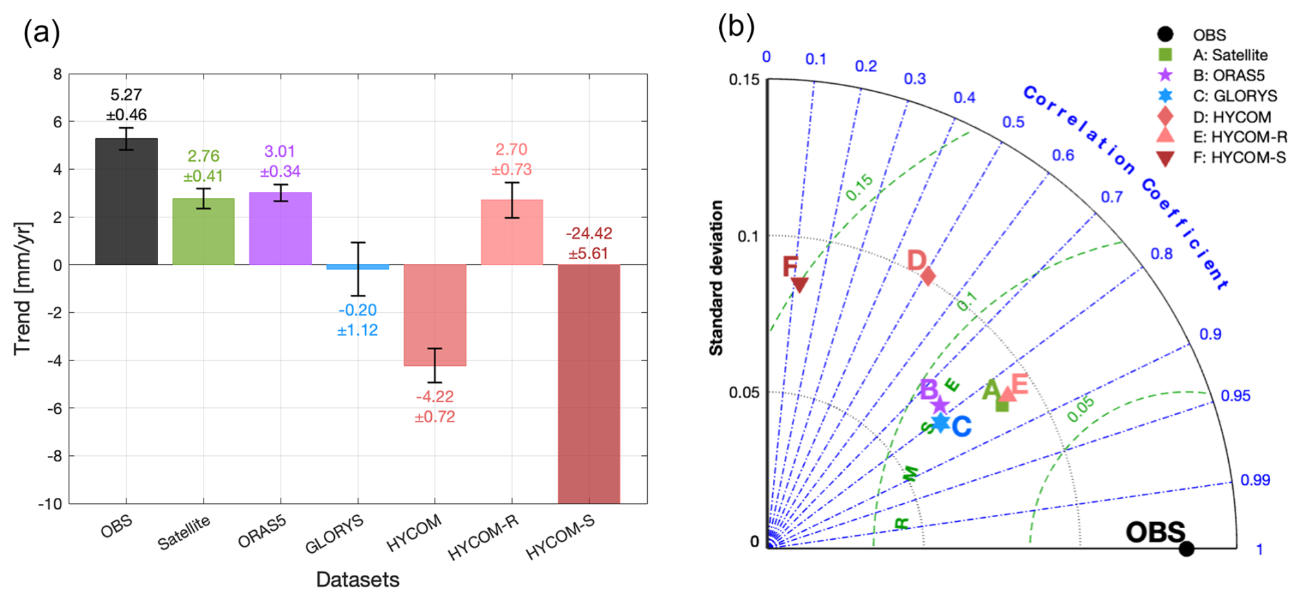
Figure 11 Bar plot with error bar (a) and modified Taylor diagram (b). The azimuthal angle represents the correlation coefficient, the radial distance indicates the standard deviation, and the semicircles centered at the “OBS” marker refer to the root mean square errors. The colors and markers indicate each dataset (black circle: observation, green square: satellite altimetry, purple pentagram: ORAS5, light cyan hexagram: GLORYS, red diamond: HYCOM, light red upward-pointing triangle: HYCOM-R, dark red downward-pointing triangle: HYCOM-S).

Second, we assessed the correlation and variability between the observation data and the other four datasets using a Taylor diagram (Fig. 11b). Among the datasets, satellite altimetry showed the highest accuracy, with a strong correlation coefficient of 0.71 and a low RMSE (0.04 m) relative to the observation. The HYCOM reanalysis showed the lowest correlation coefficient (−0.08) and the highest RMSE (0.10 m) over the entire period, indicating poor agreement. While HYCOM-R demonstrated performance comparable to satellite altimetry, HYCOM-S showed a low correlation coefficient (−0.39) and a high RMSE (0.12 m). ORAS5 and GLORYS had correlation coefficients of 0.71 and 0.76, respectively, and both had RMSEs of 0.1 m, demonstrating better agreement and accuracy than HYCOM. Overall, HYCOM performed poorly, primarily because of its inability to reproduce SLH variability after 2018 in the HYCOM-S product.

3.3 Sea-level budget assessment at I-ORS

As mentioned above, the SLH observations from the I-ORS, refined through the developed QC process, estimated an SLR rate of 5.27 ± 0.46 mm yr⁻¹. Sea level changes can be categorized into relative and geocentric sea level change, referring to the height of the sea surface relative to the sea floor and the Earth's center, respectively. Ground-based observations, such as those from the I-ORS, represent the relative sea level change. This variation is influenced by various physical processes, including sea level changes due to ocean density and circulation, i.e., the sterodynamic (STERO) effect, mass exchange between the ocean and land, i.e., the barystatic (BARY) effect, and glacial isostatic adjustment (GIA) (Gregory et al., 2019; Frederikse et al., 2020; Cha et al., 2024). In this regard, we conducted a budget analysis of each physical process that affects the SLR at the I-ORS.

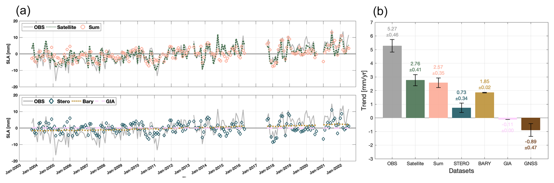
Figure 12 Monthly time series of sea level anomalies (a) and sea level rise rates (b; units: mm yr⁻¹). Each color and type of line indicates the dataset (OBS: solid black line, Satellite: dark olive dotted line, Sum: salmon pink circles, STERO: bluish green diamonds, BARY: dotted dark yellow line, GIA: dashed pale lavender line, and GNSS: dark brown).

The STERO effect is calculated as the sum of the dynamic sea level change (DSL) and the global mean steric SLR (GMSSL) (Gregory et al., 2019). DSL was estimated using ORAS5, which was also used for validation data in this study. GMSSL was derived from in situ observational datasets provided by the Institute of Atmospheric Physics (IAP; Cheng et al., 2017), the Met Office Hadley Centre (EN4; Good et al., 2013), and the Japan Meteorological Agency (JMA; Ishii et al., 2017). The GMSSL was produced using the temperature–salinity profile data from each institution and was used to compute the STERO effect by adding the DSL. The BARY effect refers to sea level rise resulting from mass contributions of ice melting from the Antarctic and Greenland ice sheets and glaciers and from changes in land water storage. For this, we used the reconstructed ocean mass data from Ludwigsen et al. (2024). The GIA accounts for sea level changes resulting from the redistribution of mass due to the melting and retreat of glaciers since the last glacial period. To estimate GIA, we used model outputs from Caron et al. (2018), who improved model accuracy by incorporating global positioning system (GPS) time series from 459 sites and 11 451 relative sea level records, as well as by computing the ensemble mean of 128 000 model simulations.

Figure 12 presents the sea level time series and trend budget at the I-ORS, along with a comparison with satellite altimetry data. The rate of SLR contributing to physical processes (Sum = STERO + BARY + GIA) was 2.57 ± 0.35 mm yr⁻¹, which is approximately 2.70 ± 0.58 lower than that of observation (5.27 ± 0.46 mm yr⁻¹). A similar discrepancy was found when comparing satellite altimetry to observation (difference: 2.51 ± 0.62 mm yr⁻¹). Among the components of physical processes, the STERO effect contributed 0.73 ± 0.34 mm yr⁻¹, accounting for approximately 28 % of the total estimated SLR. The BARY effect contributed the most, with 1.85 ± 0.02 mm yr⁻¹ (about 72 %). Meanwhile, GIA resulted in a slight sea level fall, contributing −0.11 ± 0.00 mm yr⁻¹, approximately 0.04 %.

Satellites are unable to detect vertical land motion (VLM) because they measure changes in the distance from the center of the Earth to the sea surface. In contrast, station-based observations are affected by VLM, as they measure the change in height from the seafloor to sea level (Han et al., 2014; Gregory et al., 2019; Cha et al., 2024). Hence, the difference between the sea level trend from satellite altimetry and that record at the I-ORS can be regarded as the VLM component. We examined whether the observed difference of approximately 2.51 ± 0.62 mm yr⁻¹ could be attributed to VLM. Cha et al. (2024) defined total VLM as the sum of the VLM components from GIA, BARY effects, and local processes, where GIA and BARY represent natural contributions. The GIA-related VLM was obtained from Caron et al. (2018), while the BARY-related VLM was derived from Frederikse et al. (2020). The VLM component of the local process was calculated as the difference between the sea level trend due to physical processes (2.57 ± 0.35 mm yr⁻¹) and the observed sea level trend of 5.27 ± 0.46 mm yr⁻¹. At the I-ORS location, the VLM contributions from GIA and BARY effects were calculated to be 0.22 ± 0.14 and 0.28 ± 0.64 mm yr⁻¹, respectively. In contrast, one for local processes was estimated at −2.67 ± 0.60 mm yr⁻¹. Therefore, the total VLM was approximately −2.17 ± 0.89 mm yr⁻¹, indicating that significant ground subsidence is occurring at the site, principally driven by local factors rather than natural processes.

Additionally, we analyzed the trend of the observed vertical displacement using GNSS data collected at 30 s intervals at the I-ORS from 2013 to 2019. The trend of GNSS-derived vertical displacements, based on daily means, was −0.89 ± 0.47 mm yr⁻¹ (p<0.05). Although this trend is estimated over a relatively short period and lower than the estimated VLM from the local process (−2.67 ± 0.60 mm yr⁻¹), it appears to confirm the presence of ground subsidence at the I-ORS.

4 Summary and discussion

This study developed a novel QC procedure named TALOD, based on a high-resolution tidal prediction model, and applied it to 10 min interval SLH data observed using a MIROS rangefinder (SM-140) from 2003 to 2022 at the I-ORS. The TALOD method comprises both manual and automatic processes. The manual check is performed prior to the automated procedures and flags specific sections based primarily on historical metadata to enhance the performance of subsequent automated QC steps.

The automatic process consists of range, spike, and stuck checks. The range check utilized residual components derived from the TPXO9 tidal prediction model, allowing it to address issues such as detection failure caused by non-periodic outliers or contamination during tidal component estimation through the least squares method. Spatiotemporally optimized thresholds are applied in the spike check to reduce misclassifications and detection failures, particularly those caused by frequent recurring erroneous values. By setting these thresholds using non-tidal residuals, the spike check outperforms traditional gradient-based GSM, which tends to incorrectly flag rapidly fluctuating SLH, such as extreme weather events, as outliers. For the stuck check, we incorporated the reoccurrence frequency of specific values to handle the alternation between the good and bad data, which are the unique characteristics of SLH at the I-ORS. This study confirms that the novel stuck check, which leverages the reoccurrence rate of identical values over a defined time period, can reduce truncation and increase the retention rate of valid data compared to existing QC processes.

The TALOD QC process includes the EEF, which indicates the periods when SLH is affected by extreme weather events. For instance, during typhoon-affected periods, the variance in SLH was frequently more than 4 times larger (including flagged data) than under normal conditions, increasing the likelihood that some good data may be mistakenly flagged as range or spike errors. Because sufficient observational data are essential for research on typhoon-related processes, the EEF allows researchers to selectively include these data in their analysis to investigate the dynamics of extreme weather events.

In the SLR budget analysis, the BARY effect associated with mass exchange between the ocean and land was the primary contributor, accounting for approximately 70 % of the total trend. The discrepancy in the sea level trend between observations from the I-ORS and satellite altimetry (approximately 2.67 mm yr⁻¹) can be attributed to VLM. The total VLM estimated from reanalysis data (−2.17 mm yr⁻¹) indicates considerable ground subsidence of the I-ORS site, driven by local processes rather than by natural processes. Although the estimated VLM varied depending on the reanalysis data, the GNSS-based observations of vertical displacement from 2013 to 2019 also showed a trend of −0.89 ± 0.47 mm yr⁻¹, further confirming the ongoing ground subsidence at the I-ORS.

Despite the advancements of TALOD QC, several challenges remain. The current implementation of the TALOD QC process is limited to delayed-mode SLH data and is not yet fully automated. Moreover, additional procedures are required to account for misclassification during extreme weather, such as rogue waves. In normal cases, good data with extreme values induced by the inverted barometer and steric effects may be erroneously identified as errors. Thus, a supplementary step involving the adjustment of detection thresholds using simultaneously observed buddy variables – such as air/water temperatures, wind, and sea level pressure – is required to improve accuracy.

Nevertheless, the TALOD QC process is versatile enough to be applied to both tide gauges and rangefinders. It also enhances adaptability by utilizing predicted tidal components for each location. Well-qualified in situ data are essential not only for data assimilation and validation but also for data management. The I-ORS platform stands out as a unique resource, offering more than 20 years of continuous sea level observations along with various air–sea monitoring data in the central East China Sea. Along with the I-ORS, two northern stations – Gageocho and Socheongcho ORSs – can support studies on the propagation of oceanic and atmospheric signals between marginal seas and the open ocean, ranging from extreme weather to climate variability.