Drivers of high-frequency extreme sea levels around northern Europe – synergies between recurrent neural networks and random forest

Northern Europe is particularly vulnerable to extreme sea level events as most of its large population and financial and logistical centres are located by the coastline. Policy-makers need information to plan for near- and longer-term events. There is a consensus that, for Europe, in response to climate change, changes to extreme sea level will be caused by mean sea level rise rather than changes in its drivers, meaning that determining current drivers will aid such planning. Here we determine from explainable AI the meteorological and hydrological drivers of high-frequency extreme sea level at nine locations on the wider North Sea–Baltic Sea coast using long short-term memory (LSTM, a type of deep recurrent neural network) and the simpler random forest regression on hourly tide gauge data. LSTM is optimised for targeting the excess values or periods of prolonged high sea level, random forest, the block maxima, or most extreme peaks in sea level. Through the permutation feature of LSTM, we show that the most important drivers of the periods of high sea level over the region are the westerly winds, whereas random forest reveals that the driver of the most extreme peaks depends on the geometry of the local coastline. LSTM is the most accurate overall, although predicting the highest values without overfitting the model remains challenging. Despite being less accurate, random forest agrees well with the LSTM findings, making it suitable for predictions of extreme sea level events at locations with short and/or patchy tide gauge observations.

1 Introduction

About 50 million people live by the coast in Europe (Neumann et al., 2015). In northern Europe in particular, many strategically crucial financial and logistical hubs are also located by the coast, making population and infrastructure vulnerable to extreme sea level events (see the review by van de Wal et al., 2024, and references therein). As the global climate warms and the sea level rises, extreme sea level events are projected to increase in both magnitude and frequency, especially on the North Sea and Baltic coasts (Vousdoukas et al., 2017). As recently reviewed by Melet et al. (2024), there is a consensus that this increase is driven by the shifting baseline of sea level rise rather than by changes in the mechanisms driving the extreme events. This means that identifying these drivers now would aid policy-makers in better planning of near-term (van den Hurk et al., 2022) and longer-term (Groeskamp and Kjellsson, 2020) needs for coastal defences.

The drivers of sea level in northern Europe have been extensively studied with hydrodynamic modelling (see the review in Melet et al., 2024). These models showed that, from seasonal to multi-decadal scales, variability is primarily controlled by the atmosphere, especially westerly winds (e.g. Frederikse and Gerkema, 2018; Tinker et al., 2020). Due to the models' coarse resolution, especially for the atmosphere, data-driven approaches are more adapted for shorter timescales. Using daily altimetry data over a small region of the North Sea, Sterlini et al. (2016) found a similar relationship between sea level and zonal winds but also that the wind component most important for sea level is strongly dependent on the coast's geometry. Sterlini et al. (2017) expanded their region of study to the entire North Sea and found likewise that, for daily sea level, the location influenced whether meteorological or steric components mattered most. From hourly tide gauge data, Marcos and Woodworth (2017) found the same strong relationship between the steric component and extreme sea level values (although they did not investigate any possible relationship with atmospheric variables).

Globally, some tide gauge records date back to the mid-1800s (Haigh et al., 2023). This data richness means that data-driven approaches involving machine learning are an obvious choice for sea level research. Most often, these methods aim to forecast non-tidal residuals, using atmospheric parameters as predictors. For example, Ishida et al. (2020) reproduced hourly tide gauge data in Osaka, Japan, using a type of recurrent neural network called long short-term memory (LSTM; see Sect. 2.4) and reanalysis-based time series of wind speed, wind direction, sea level pressure, and air temperature, together with global air temperature as a remote global warming forcing. Hieronymus et al. (2019) used a similar approach for nine tide gauge stations on the Swedish coast, except that they used the full spatial fields of the reanalysis variables instead of time series and showed that the 36 h forecasts they generated were faster and more accurate than those of the best European hydrodynamics model. Using the HIDRA2 (Rus et al., 2023) encoder-based deep network to forecast sea level at five tide gauge stations along the Estonian coast, Barzandeh et al. (2024) found the same result: machine learning methods produce better forecasts that are faster than those of state-of-the-art hydrodynamics models. They do note that the network struggles to reproduce high-frequency variability, producing overly smooth time series, a result that Tadesse et al. (2020) also found for daily sea level globally using random forest.

Predicting extreme values is not a problem unique to sea level, and therefore the development of machine-learning-based methods adapted to extreme values is ongoing for many climate applications. One main direction is to use convolutional neural networks on spatial fields, e.g. for predicting extreme winds (Jiang et al., 2022a), precipitation (Wilson et al., 2022), sudden stratospheric warming events (Strahan et al., 2023), or tropical cyclones (Ascenso et al., 2024). These topics benefit from the fact that researchers can somewhat easily augment their data by rotating their images, hence generating new training points (Ascenso et al., 2024). This cannot be done for 1D time series analysis, which instead preferably uses LSTM. Recent examples of this include predicting European river flooding (Jiang et al., 2022b), storm intensity on the French Atlantic coast (Frifra et al., 2024), or extreme precipitation at specific locations in China (Tang et al., 2022). Note that Tang et al. (2022) also used random forest.

What all of these studies have in common is that their main objective is to predict extremes rather than identify what drives them, even though both LSTM and random forest can be made explainable. They also often rely on networks that are overly fitted to a specific location and therefore of limited use to a wider region. Here we develop LSTM and random forest models to predict and identify the drivers of sea level around the wider North Sea and Baltic Sea regions, using hourly tide gauge data as predictands and atmospheric and hydrological time series as predictors, focusing on extreme sea level only, as we describe in Sect. 2. We present the results of the LSTM- and random-forest-based analyses in Sect. 3.1 and 3.2, respectively, before discussing their applicability to sea level monitoring and coastal defence planning in Sect. 3.3.

2 Methods

2.1 Hydrographic, meteorological, and hydrological data

We use hourly tide gauge data from nine stations around northern Europe (Fig. 1a): three on the North Sea coast (station names Lowestoft, Den Helder, and Esbjerg), three in the Baltic (Ratan/Umeå – hereafter referred to as Umeå –, Helsinki, and Gedser), and three in the transition between the two seas, i.e. the Skagerrak/Kattegat (Oslo, Gothenburg/Göteborg, and Klagshman/Malmö, hereafter referred to as Göteborg and Malmö, respectively). For each region, we tried to select locations that are major population centres but had to compromise in order to obtain long enough, uninterrupted time series (Table 1). We also excluded cities where the water level is artificially controlled by humans, such as London or Rotterdam, which have flood defence systems, or Stockholm, which is fed by a reservoir lake. For the three Swedish cities Göteborg, Malmö, and Umeå, the tide gauge data were provided by the Swedish Meteorological and Hydrological Institute; for the other locations, we used the Global Extreme Sea Level Analysis (GESLA) dataset version 3, last updated in November 2021 (Woodworth et al., 2016; Haigh et al., 2023).

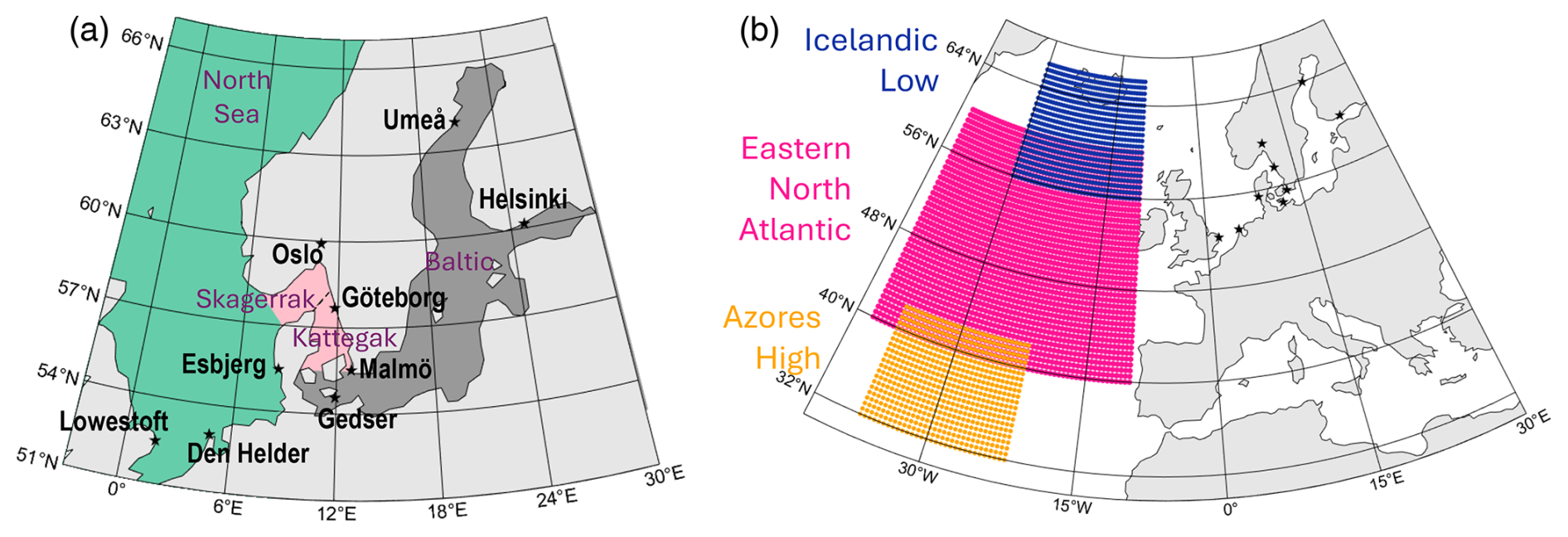
Figure 1 (a) The nine cities of this study, chosen for their data availability and to cover the three main maritime regions: the North Sea (green), the Skagerrak/Kattegat (salmon), and the Baltic (grey). (b) Regions used for the creation of the remote predictors: the Icelandic Low (blue) and Azores High (orange) sea level pressure and the eastern North Atlantic (pink) sea surface temperature.

To determine the potential drivers of extreme sea level, we use meteorological and hydrological data. Ideally, we would have used meteorological time series from weather stations co-located with the tide gauge stations. Unfortunately, those are often at different locations, their distribution managed by different services, and their obtention requiring one to speak the language of the country in order to understand the download interface. In addition, the time series are often patchy, missing data at different times to the tide gauge stations. Therefore, we opted to use ERA5 instead (Hersbach et al., 2020). The spatial resolution is 0.25° and the temporal resolution hourly; the time period covered 1 January 1940 to 31 December 2023. We use the hourly 10 m u and v components of the wind, evaporation, total precipitation, mean sea level pressure, and sea surface temperature. Wind and sea level pressure have a dynamic effect on the sea level; evaporation and precipitation change the amount of water available and, along with sea surface temperature, contribute to the steric sea level. We compute the wind speed and direction from the u and v components. As we want to determine the feasibility of predicting sea level from in situ stations, for each city and variable, we use the time series of the ERA5 grid cell closest to the tide gauge station coordinates as provided by the Swedish Meteorological and Hydrological Institute (SMHI) or GESLA, similar to what Ishida et al. (2020) did. We also generate the hourly time series of three “remote” drivers, representing the state of the wider North Atlantic climate and its storminess:

• the hourly spatial-minimum sea level pressure around Iceland (Fig. 1b, blue), longitudes −30 to −10° E and latitudes 56 to 66° N;

• the hourly spatial-maximum sea level pressure around the Azores (Fig. 1b, orange), longitudes −37 to −22° E and latitudes 32 to 42° N; and

• the hourly spatial-mean sea surface temperature over the eastern North Atlantic (Fig. 1b, pink), longitudes −40 to −10° E and latitudes 40 to 60° N.

Note that combining the Icelandic Low and Azores High time series yields the North Atlantic Oscillation index (e.g. Hurrell, 1995).

Table 1 Maximum time period for which the hydrographic data are available for each city, together with the corresponding hydrological data: river names, river station numbers in the Global Runoff Data Centre (GRDC), and common time periods of the rivers if there is more than one. See the Methods and “Data availability” sections. Note that “n/a” stands for “not applicable”.

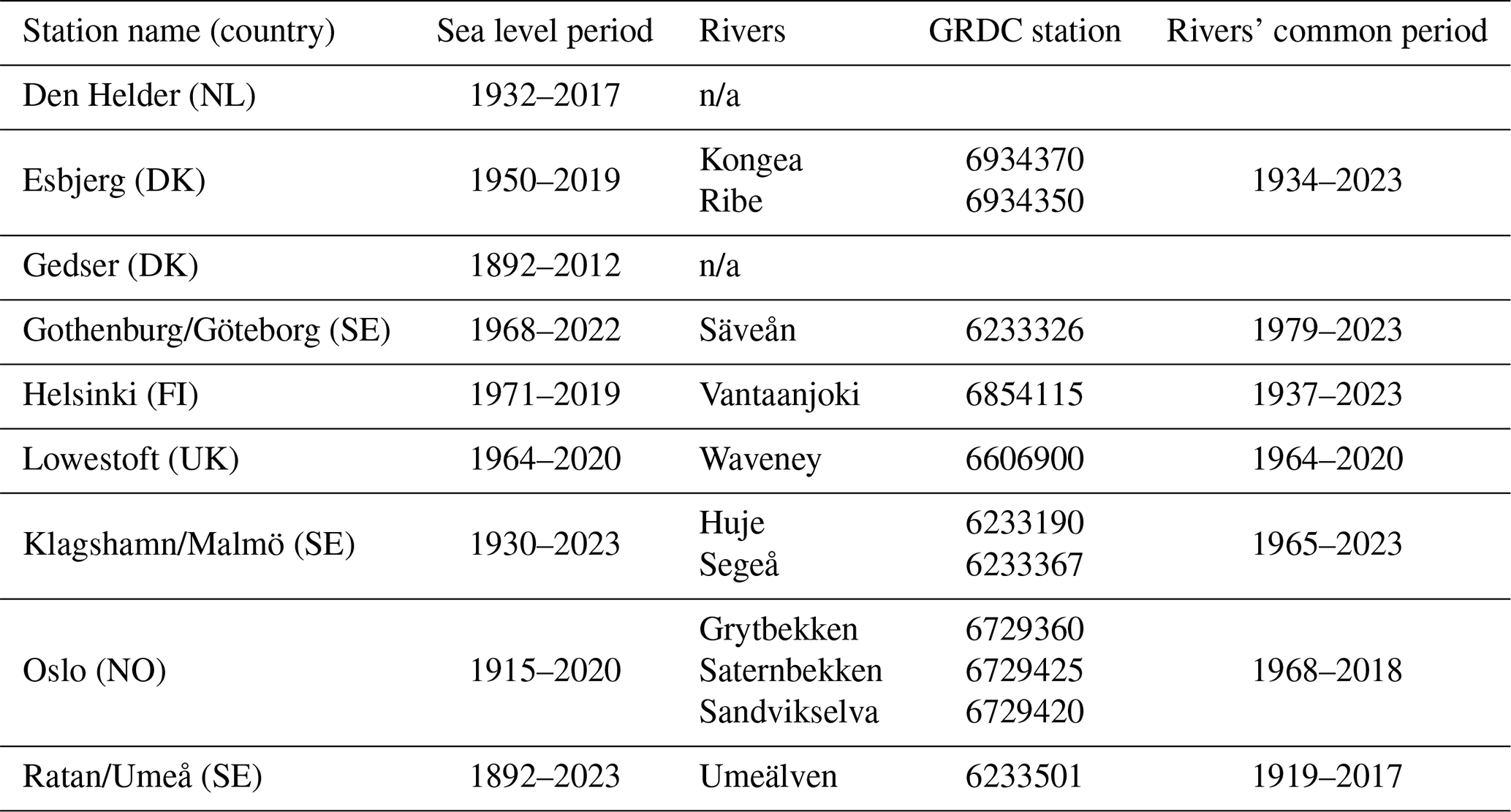
The last potential driver of extreme sea level used in this study is hydrological. Data obtention and quality issues are similar to those of the meteorological data described in the previous paragraph. We therefore use the river discharge time series from the Global Runoff Data Centre (GRDC). We manually selected the station(s) of the rivers that discharge in the city; some had none, and some had up to three (Table 1). The GRDC data are daily, meaning that we linearly interpolated them to generate hourly data. We acknowledge that daily mean data are not ideal for detecting and predicting extreme hourly values of sea level, and we can only lament the fact that hourly products are not available. Even as daily means, hydrological data often have a shorter time coverage than hydrographic ones (Table 1); for the few locations around Sweden where we found hourly data, their time coverage was too short and patchy to be of use.

2.2 Further data preparation

We de-tided the tide gauge data using the UTide package for MATLAB (Codiga, 2024). Although some machine learning methods have used the tide gauge data, including their tide signal (e.g. Rus et al., 2023), we chose to remove them as they are the predictable part of the signal, and we are interested in explaining the rest.

All of the datasets have been detrended, assuming a linear trend and using a 95 % significance threshold. The exceptions are the u and v components of the wind, which were first split into their positive (westerly or southerly) and negative (easterly or northerly) parts such that

$$\begin{array}{}\text{(1)}& \left\{\begin{array}{l}{u}_{+}=u\text{ if }u>\mathrm{0},\\ u_{+}=\mathrm{0}\text{ otherwise,}\end{array}\right.\end{array}$$

and

$$\begin{array}{}\text{(2)}& \left\{\begin{array}{l}{u}_{-}=\mathrm{0}\text{ if }u>\mathrm{0},\\ u_{-}=u\text{ otherwise.}\end{array}\right.\end{array}$$

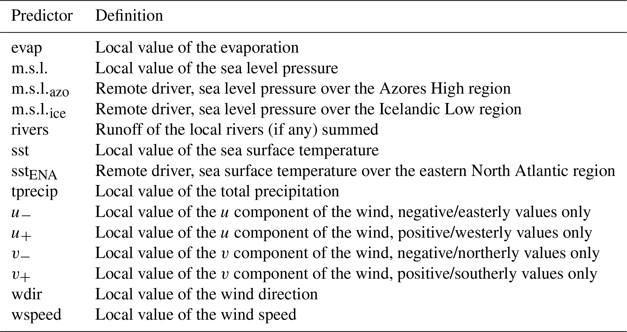
Then these positive and negative components were detrended and used as predictors instead of the u and v components. The other exception is the wind direction, which was not detrended. We purposely keep variables that are correlated with each other (see Table A1) to test compound events. We acknowledge that this may result in an underestimation of the importance of the individual predictors. The correlations will be discussed in the Results section when relevant. The predictor short names and their definitions are summarised in Table 2.

Table 2 Summary of the 14 predictors used in this study, by alphabetical order of the short names used in the figures. See Fig. 1 for the region definitions and Table 1 for the rivers.

As we describe in Sect. 2.4, we use these data in two types of machine learning models: LSTM and random forest. Random forest requires no data normalisation, so the variables are used directly after de-tiding and detrending. For LSTM, we use a min–max normalisation so that all variables are between 0 and 1. Prior to normalisation, we convert all of the time series to their absolute values; this only affects u₋ and v₋. This is to preserve their shape as zero-inflated, heavy-tailed distributions after normalisation, similar to that of the other variables.

All of the datasets are in UTC; no re-timing is needed. Any missing value in the hydrographic or hydrological series was set to 0. We only select the time period common to all three data sources (Table 1; ERA5 is 1940–2023). The shortest period is 43 years for Göteborg; the longest is 77 years for Den Helder and Umeå.

2.3 Extreme sea level events – definitions

Two types of events are investigated here:

• peaks in sea level, or absolute maxima of a given block, for which random forest is most suited (see the Introduction section); and

• prolonged periods of high sea level, for which LSTM is most suited.

For the first type of event, we select all values in excess of the mean sea level plus 3 standard deviations (or above 0.75 in the normalised series used for illustration in Fig. 2). We use a block size of 7 d: that is, if more than one value is above the threshold within a 7 d period, we only select the maximum value. For all of the cities, we obtain 200 to 300 events during the time period common to all three types of variables (black stars in Fig. 2).

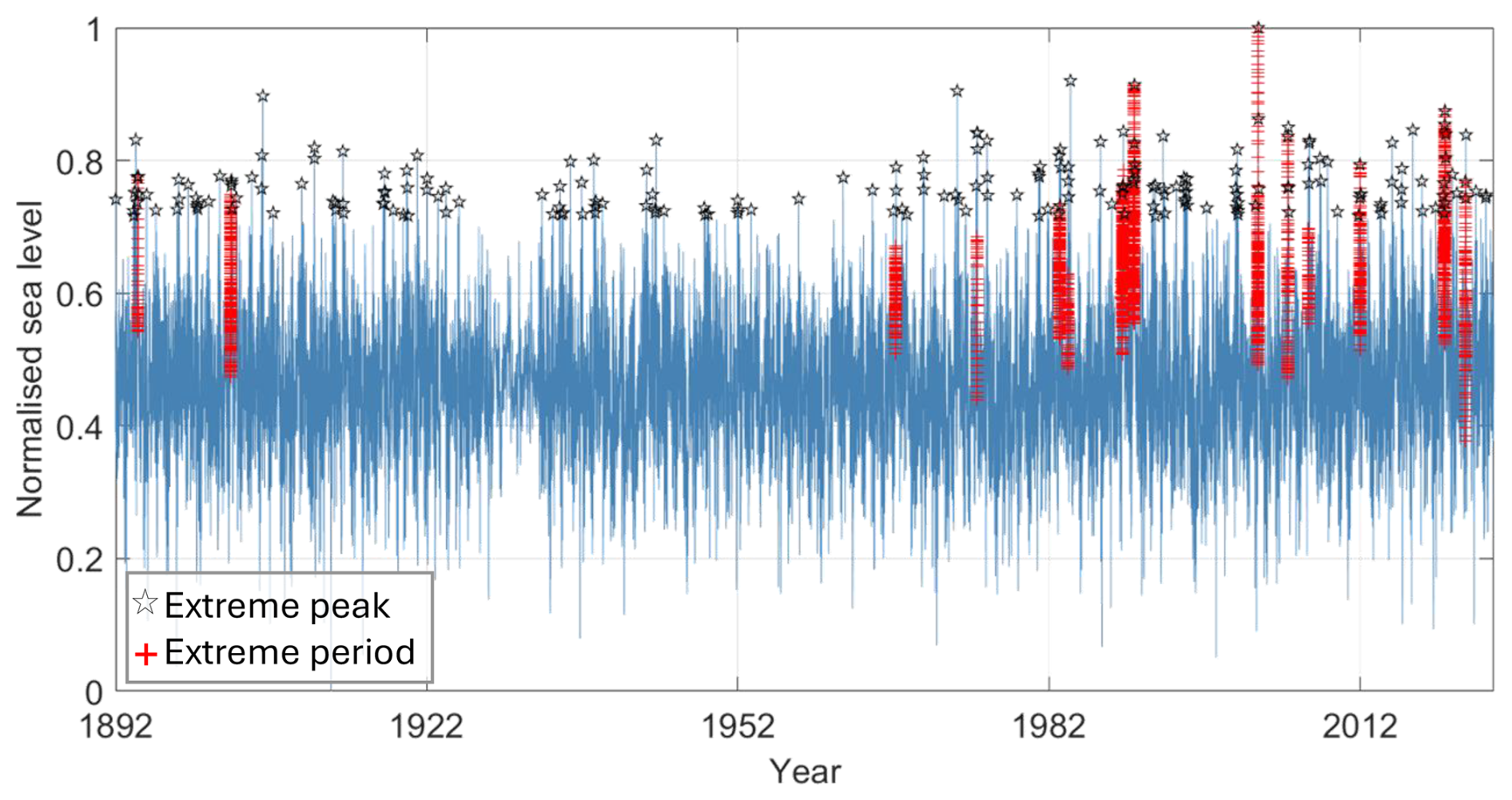
Figure 2 Illustration of the two extreme sea level detection methods, using the complete time series of sea level for Umeå min–max-normalised after de-tiding and detrending. The 212 black stars are the hourly values detected as peaks and the 5828 red crosses the hourly values detected as belonging to a period of high sea level. The actual detection is done on the shortened time series and on the non-normalised series for the peaks (see the text).

For the second type of event, we first compute the 30 d running mean time series and then select the values in that running mean series that are above its mean plus 3 standard deviations. The value of 30 d was chosen as a compromise: it yields enough points for training, it is long enough compared to our hourly data according to extreme value theory (Ólafsdóttir, 2024), and it is longer than the memory of the system (2–3 d, Hieronymus et al., 2019). For all of the cities, we obtain several thousand hourly data points during the time period common to all three types of variables (red crosses in Fig. 2).

2.4 Machine learning models: LSTM and random forest

2.4.1 LSTM and permutation feature importance

Sea level is the result of current and past cumulative forcings. To take this temporal dependency into account, we use the type of recurrent neural network (RNN) called long short-term memory (Hochreiter, 1997). A standard RNN uses as input not only the predictors at the same time step as the target, but also its hidden state variables of the previous time step. Each time the network moves forward, the hidden state is overwritten. LSTM in contrast uses a set of “gates” to regulate which information is forgotten and which is stored and passed as input, allowing the network to build a sophisticated combination of all of the past time steps that it considers relevant.

We split the detrended, normalised time series, merging the prolonged periods of high sea level into a validation set (first 15 %), a test set (second 15 %), and a training set (last 70 %). We performed a hyperparameter search on the Göteborg time series using the following hyperparameter space:

• window size 2, 3, 6, 12, 18, 24, 36, 48, 72, 120, and 168 h;

• number of layers 1, 2, 3, 4, and 5;

• number of units per layer 10, 20, 33, 50, 100, and 200;

• learning rate 0.001, 0.005, and 0.01;

• batch size 20, 50, and 100; and

• dropout rate 0.005, 0.01, and 0.015.

After this hyperparameter search, we settled for a network with three LSTM layers with a hyperbolic tangent activation function of 100 units each and one dense layer with a dropout rate of 0.015 in between each layer. We used the Keras Python package (Chollet and The Keras Team, 2015). The input batch size is 20, and the network's overall learning rate is 0.01. We found the best performance with a window of 12 h, except for Helsinki (24 h) and Malmö (36 h). These short windows were expected given that extreme sea level is a short-lived event, and they are consistent with the findings of Hieronymus et al. (2019) for the Swedish coast. The performance for Helsinki was markedly improved by using 10 units per layer and a batch size of 100. These settings minimised the mean square error while resulting in a correlation between the target and the predicted value of at least 0.81, i.e. explaining more than two-thirds of the signal. For each city we then generated 100 models with a random initial state and selected the best model following these steps:

• The models have equally good mean square errors by design. We prioritise those that successfully explain most of the signal and therefore select the subset of models with a correlation within 0.2 of the maximum correlation of all 100 models.

• Within this subset, we rank the models based on their overall root mean square error (RMSE) but also their RMSE for normalised sea level values larger than 0.66, as we noticed during training that LSTM struggled to reproduce these high values without overestimating the rest of the series.

• We select the model with the lowest sum of these two ranks; at equal value, we take the one with the highest correlation.

To determine the contribution of each predictor to the overall prediction, we perform a permutation feature importance test. That is, for each predictor, we run the model again after having set this predictor to an array of random values. The difference between the explained variance (correlation squared) of the default prediction and that with the random values directly gives the contribution of that predictor to the signal's variance.

2.4.2 Random forest and feature importance

To investigate the peaks in more detail, we move away from neural networks and instead use a method that is simpler but more adapted to point measurements: a random forest regression. Random forest is an ensemble of decision or regression trees, which makes it a preferable method for identifying the drivers of sea level as the trees directly choose the most relevant predictors at each split. The random forest feature importance is calculated using the Gini importance measure. An inconvenient aspect is that the feature importance returned by the trees is relative to the parameters used in the model, unlike that of LSTM, which is absolute. Another limitation of random forest is that temporal relationships are not considered, even though we know that sea level does not only depend on synchronous forcings. We remedy this by providing as input the predictors (listed in Table 2) at the same hourly time step as the target sea level values, but also 1, 3, 6, 12, 24, and 48 h as well as 3, 5, and 7 d prior, resulting in a total of 140 predictors.

We randomly split the values into a training set (80 %) and a test set (20 %). Here too we performed a hyperparameter search on the Göteborg series, with the following hyperparameter space:

• number of trees 100, 200, 500, 1000, and 2000;

• number of splits 1, 2, 3, and 4;

• number of leaves 2, 3, 4, and 5;

• bootstrapping true or false; and

• if bootstrapping true, maximum number of samples 0.1, 0.2, 0.5, 0.75, and 1.

After this hyperparameter search, we chose the settings that minimised the square error, which was 200 trees with a minimum of two leaves (minimum leaf samples) and four splits (minimum split samples), with bootstrapping or “bagging” set to true and the maximum number of samples set to 0.5 (maximum samples). The optimum settings and results were the same when minimising a weighted mean error to favour the most extreme values instead. We used the Python package Scikit-learn (Pedregosa et al., 2011). To determine the contribution of each predictor to the overall prediction, we used the built-in regression feature estimator, limiting the selection to 35 features (i.e. one-fourth of all those possible). For each city we produced an ensemble of 100 models with feature estimation and analysed their mean results.

3 Results and discussion

3.1 North-westerly winds contribute most to periods of prolonged high sea levels

Starting with LSTM applied to periods of high sea levels, the correlation between the test dataset and its predicted values is 0.8 or higher for all of the cities (correlation squared in Table A2). The root mean square error between the test and prediction is around 5 % for all of the locations except Esbjerg (9 %, Table A3). Likewise, the root mean square error for only the highest third of the values is around 2.5 % for all of the locations except Esbjerg (4 %, Table A4). We could not see an obvious reason for Esbjerg's difference, and the RMSE there remains acceptably low, so we do not investigate this further.

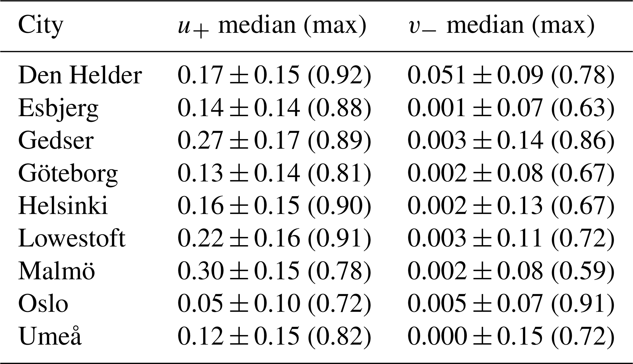
The feature permutation from LSTM directly returns the absolute contribution of each predictor to the variance of the signal. Unsurprisingly, for all of the cities and all of the predictors, the explained variance is less if a predictor is set to random values instead of its series (bottom-left triangles in Fig. 3, Table A2). On average, the northerly and westerly winds v₋ and u₊ are the first- and second-most important predictors for the majority of the cities, with v₋ contributing more than 50 % of the signal in Gedser, Helsinki, and Lowestoft (dark red in Fig. 3). Interestingly, these wind values themselves are not extreme over the periods used by LSTM (Table 3): for all of the cities, the median of their normalised values is low to very low, but the series also includes normalised values larger than 0.9. That is, contrary to expectations, the westerly and northerly winds are not anomalously weak or strong during periods of prolonged high sea level. This demonstrates the strength of LSTM, which is capable of detecting patterns beyond the usual human statistics.

Table 3 For each city, median ± standard deviation, and maximum value in parentheses, the normalised westerly u₊ and northerly v₋ wind subsets of the complete time series used as predictors for LSTM are shown. The normalisation was done on the complete time series.

Most of the predictors are important for some cities but negligible for others. The local evaporation for example contributes 38 % of the variance in sea level for Gedser, 10 % and 1 % for Helsinki and Umeå (the other two cities in the Baltic), and 0 % for Malmö, the nearest neighbour. In addition, in all these cases the evaporation is only weakly or not at all correlated with the other predictors (Table A1). That is, its signal is not diffused within the other predictors. Overall, the importance of a predictor is not similar for cities in the same sea, and the importance of remote predictors does not increase with proximity to their source (e.g. $\mathrm{m}.\mathrm{s}.\mathrm{l}{.}_{\mathrm{ice}}$ contributes 5 % to Umeå and 2 % to Den Helder).

For some predictors, their contribution is negligible regardless of the city, i.e. lower than 10 %. This is the case with e.g. $\mathrm{m}.\mathrm{s}.\mathrm{l}{.}_{\mathrm{azo}}$ or the southerly winds v₊, which is not surprising given that these variables are rather indicative of good weather conditions over the region, or with the rivers with the exception of Oslo (19 %), which may be because of their original daily resolution. These variables are not strongly correlated with any of the strong predictors either (Table A1). Similarly, the strong contribution of sst_ENA to Umeå and nowhere else, along with the low correlation of sst_ENA with anything except the local sst, suggests rather that we are missing a potential driver for Umeå that could be correlated with sst_ENA, such as the sea ice concentration or thickness. Unfortunately for weather observations, the simpler-to-monitor compound variables (m.s.l., wdir and wspeed) do not contribute significantly more than the individual predictors.

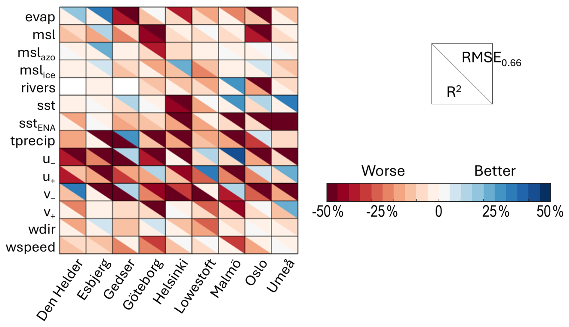
Figure 3 For each city on the x axis, using LSTM, the change in the explained variance (R², bottom left) and the root mean square error of the normalised sea level values larger than 0.66 (RMSE_0.66, top right) between the default run with all of the predictors and that where the one predictor on the y axis was set to random values are shown. Red means that the sea level prediction is worse when the predictor is randomised, blue that the prediction is improved. See Table 2 for the predictor definitions. For readability, we actually show RMSE_0.66 normalised by the value of the default run. See Tables A2–A4 for the actual values.

Using the root mean square error of the entire prediction set yields broadly the same results as using the explained variance (Table A3). Using that of the highest sea level values RMSE_0.66 by contrast gives surprising results: some predictions are improved when a predictor is replaced with random values (blue top-right triangles in Fig. 3, Table A4). In most cases, this predictor did not contribute much to the explained variance anyway, such as the evaporation for Den Helder or Esbjerg (contributions to the variance R² of 3 % and 1 %, respectively; RMSE_0.66 improved by 19 % and 33 %, Fig. 3) or the rivers for Malmö (R² of 3 %; RMSE_0.66 improved by 30 %). These are not strongly correlated with other variables (Table A1), so this is not an artefact of our method. More surprisingly, there are also six cases where the north-westerly winds are the main contributors to the time series, as described in the previous paragraph, yet removing them improves the prediction of the highest sea level values. For v₋, these are Den Helder, Gedser, and Malmö; for u₊ they are Göteborg, Lowestoft, and Oslo (Fig. 3).

Our results suggest that periods of prolonged sea level and peaks in sea level have different drivers, at least in our region of interest. We investigate this further in the next section, focusing on the individual most extreme values in sea level for each city. We also move to a method more adapted to point measurements: random forest regression.

3.2 The main drivers of the most extreme peaks depend on the coastline's geometry

For the extreme peaks of sea level, as expected from the literature (see the Introduction section), the performance of random forest when including all predictors is slightly lower than that of LSTM for the prolonged periods of high sea level. The average root mean square error is less than 20 cm for all of the cities (Table A5) compared to an average non-normalised sea level anomaly of more than 1 m. The correlation between test and predicted series is around 0.8, except for Helsinki and Oslo, where it is 0.7. This lower correlation is most likely because the sea level depths in these cities' respective bay and fjord are influenced by local weather processes that are not captured by ERA5's comparatively coarse resolution.

For the extreme peaks of sea level at all of the locations, there is no predictor in the random forest model that stands out as most important (Fig. 4), unlike the results for the periods of high sea level. In fact, the most important drivers at each location seem related to the local coastline geometry and geography:

• For Den Helder, Esbjerg, Göteborg, and Lowestoft, the westerly wind (u₊) is most important. This is probably because all these locations are relatively close to the source of the main Atlantic storms, especially so Lowestoft. For Den Helder and Esbjerg, this finding is in agreement with Sterlini et al. (2016), who argued that westerly winds indirectly matter because of induced Ekman transport that accumulates water on the coast. In the case of Esbjerg and Göteborg, the north–south orientation of the coastline also makes it vulnerable to westerly winds.

• For Gedser and Malmö, the northerly wind (v₋) is most important, which most likely is because it controls the flow of water between the Kattegat and the Baltic or because both stations are protected from the westerlies by extensive land to the west (Fig. 1).

• For Helsinki and Oslo, it is the local sea level pressure (m.s.l.) that is most important, probably because both locations are located deep in their respective fjord or bay, and therefore they are sheltered from the wind or the wind components from ERA5 are not representative of the extreme local weather that can develop in fjords.

• For Umeå, southerly wind (v₊) and precipitation are most important. Similar to Gedser and Malmö, the meridional wind most likely matters because Umeå lies on the western coast of its sea and therefore is not affected by westerly winds. Alternatively, since the network also has high importance for precipitation, it could be because southerly winds bring warm moist air there.

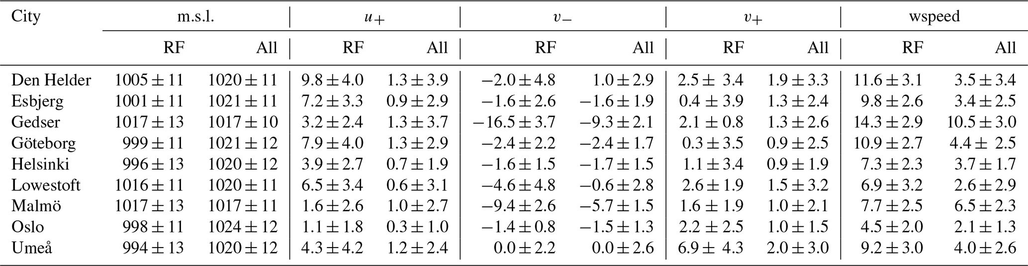
Unlike for LSTM, the values of the predictor variables at these locations are noticeably different during the peaks of extreme sea level compared to the rest of the time series (Table 4). The westerly wind is more than 5 times stronger than usual for Den Helder, Esbjerg, Göteborg, and Lowestoft (medians larger than 6 m s⁻¹ compared to the usual 1 m s⁻¹). For Gedser and Malmö, the northerly wind is more than twice as strong, reaching a median of 16.5 m s⁻¹ for Gedser. The sea level pressure is anomalously low in Helsinki and Oslo, with medians lower than 1000 hPa. Umeå is the one city with anomalous southerly winds more than 3 times as strong as usual. Additionally, for most of the cities, the wind speed is anomalously high (Table 4). This may be why LSTM could not predict the most extreme sea level values well: the predictands have a different distribution at these peaks.

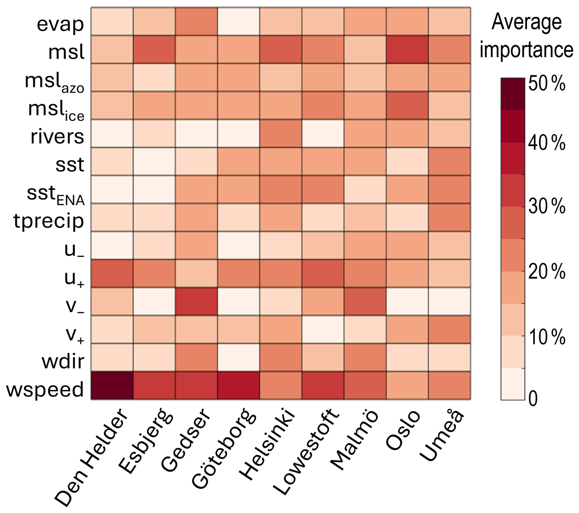
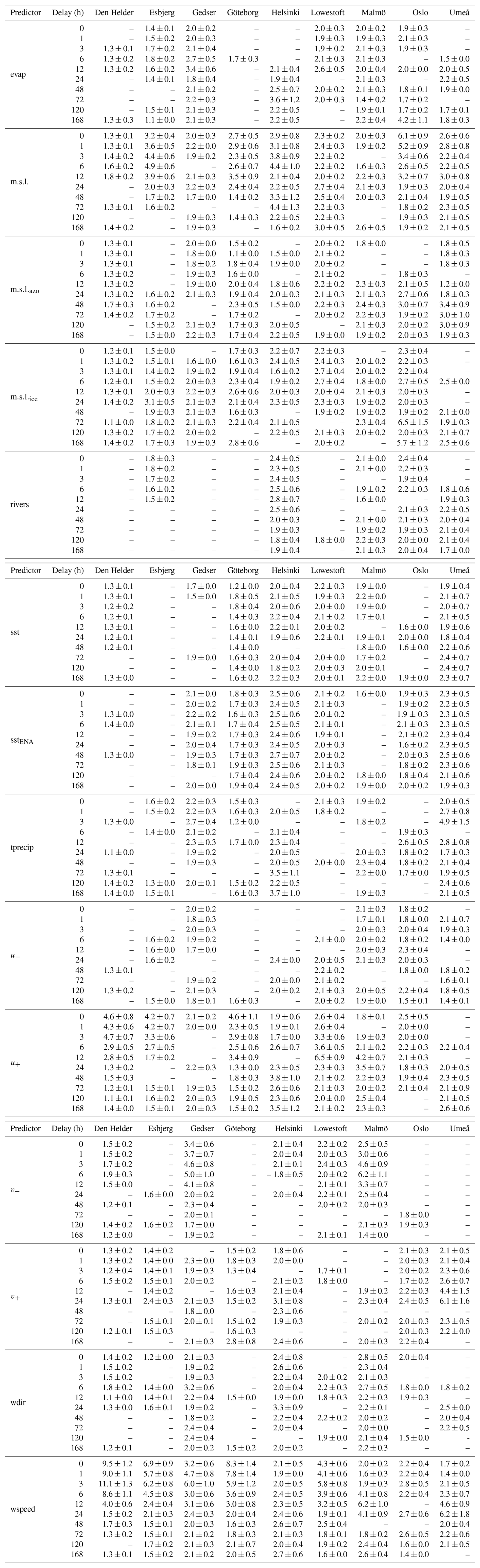
Figure 4 For each city on the x axis, using random forest for each predictor on the y axis, the average importance over the 100 runs is summed for all of the predictors' delays (i.e. simultaneous values and nine delays). See Table 2 for the predictor definitions. See Table A6 for the individual values for each delay rather than the sum and the ensemble standard deviations.

Table 4 For each city, the median ± standard deviation of the sea level pressure (m.s.l., hPa) and the westerly (u₊, m s⁻¹), northerly (v₋, m s⁻¹), and southerly (v₊, m s⁻¹) winds and wind speeds (wspeed, m s⁻¹) for the subsets of the complete time series used as predictors for the random forest (“RF” columns, left) are compared to the complete time series (“All” columns, right).

In agreement with Sterlini et al. (2017), the steric component, represented here by the local sea surface temperature (sst, Fig. 4), is important for some locations but not as important as the meteorological component. Similarly, the remote drivers seem more important than for the periods of prolonged sea level: both $\mathrm{m}.\mathrm{s}.\mathrm{l}{.}_{\mathrm{azo}}$ and $\mathrm{m}.\mathrm{s}.\mathrm{l}{.}_{\mathrm{ice}}$ have some importance at all of the locations, which is consistent with the importance of their combined index, the North Atlantic Oscillation, for extremes in the region (Hurrell, 1995; Melet et al., 2024). sst_ENA, which can be considered a proxy for overall warming, also has a relative importance of more than 20% for more than half of the locations, which is consistent with the local relationship between global warming, the mean sea level value, and extreme sea levels (Vousdoukas et al., 2017).

Finally, it is worth noting that the LSTM results when using the error on the high sea level values (RMSE_0.66 in Fig. 3) and the random forest results (Fig. 4) agree quite well. There is a minority of cases where removing the predictor from LSTM improved the performance, even though that predictor is deemed important by random forest (blue triangles in Fig. 3 and red boxes in Fig. 4, e.g. sea level pressure for Esbjerg or westerly wind for Lowestoft). However, in most cases, either the two methods agree that the predictor is important for extreme values (red in both figures, e.g. rivers for Helsinki or wind speed for Malmö) or they both agree that it is not and can or should be removed from the prediction (blue in Fig. 3 and pale in Fig. 4, e.g. evaporation in Den Helder or $\mathrm{m}.\mathrm{s}.\mathrm{l}{.}_{\mathrm{azo}}$ in Esbjerg). Therefore, the two methods are more complementary than they first appeared, as long as one chooses the most relevant evaluation metric for LSTM.

3.3 Applicability to sea level monitoring

We confirmed, with a data-driven approach and at a higher temporal resolution, that the hydrodynamics models were correct: extreme sea level around northern Europe is primarily a result of westerly winds (Melet et al., 2024, and references therein). This is excellent news since hydrodynamics models, despite their many property and process biases, are to date the best tools for projecting future sea level (Vousdoukas et al., 2017) and its impacts (van de Wal et al., 2024) and therefore informing policy-makers. By developing two machine-learning-based methods for different situations, we provide a cheaper and faster (Hieronymus et al., 2019) alternative for shorter-term decisions. Although we did not test this here, it should be feasible to detect an upcoming extreme peak during a period of high sea level using the disagreement in predictor importance between the two methods during such peaks. Since we worked with the non-tidal residuals of sea level, this method should remain functioning even as the background sea level increases (Melet et al., 2024) and tides keep on changing non-linearly (e.g. Idier et al., 2017; Schindelegger et al., 2018), as long as no tipping point of the climate system changes the importance of the extreme sea level drivers. One might however have to change the definition of the remote drivers as air and oceans warm and storm tracks shift (Shaw et al., 2016). Future work could also consider developing a hybrid LSTM–random forest model for extreme sea level, as was done recently for weather forecasting (Magesh et al., 2024).

Although this is common practice (e.g. Hieronymus et al., 2019; Ishida et al., 2020; Jiang et al., 2022b), a limitation of this study is the use of reanalysis data instead of meteorological observations. Reanalyses, and ERA5 in particular, are known to underestimate extreme values (Bell et al., 2021), and they provide multi-kilometre average values instead of those at the location of the tide gauge station. Unfortunately, most tide gauge stations do not have co-located meteorological observations. This is even worse for hydrological observations, which are not at the same location, and, in this study, for daily averages instead of instantaneous values. This is probably the reason, surprisingly and contrary to common knowledge, why our models found that rivers are not important for extreme sea level. There are also observations that we wish we could have included but which, to the best of our knowledge, do not exist for the long time period needed for the training, such as the sea ice for Umeå. This could explain why our predictions never explained all of the variance in the time series. However, since all of our LSTM predictions explained more than two-thirds of the signal, we are confident that we included the main predictors. Relocating or creating new observation stations is a policy decision. Policy-makers should also consider whether to relocate or create new tide gauge stations, as the current ones are often at locations sheltered from waves (Melet et al., 2024). We observed that they are sometimes located so deep in the city centre that the sea level becomes too artificial to be predicted by atmospheric variables, such as in Bergen on the south-western Norwegian coast (not shown). Depending on local vulnerabilities or flood defence systems, other locations on the nearby coast might be more representative (van de Wal et al., 2024).

Although our data covered three seas and some stations were relatively close to each other, we did not find any regional coherence at the hourly timescale, unlike what was found by Poropat et al. (2024) for the monthly variability. In fact, locations with similar coastline geometry behaved very similarly. We acknowledge that our region is comparatively large for a machine learning study where single tide gauge (Ishida et al., 2020) or single sea (Ayinde et al., 2023; Ruić et al., 2025) series are the norm but still too small for us to dare extrapolate our findings too much. In the Baltic, Hieronymus et al. (2019) and Barzandeh et al. (2024) demonstrated the potential of LSTM and CNNs on the western and eastern coasts, respectively. However, on a larger scale, data scarcity remains the limiting factor. Although the RMSE was significantly larger for random forest, amounting to up to 20 % of the sea level value compared to less than 5 % for LSTM, we still recommend using random forest when tide gauge observations are short and/or patchy, as we showed that random forest can work well with individual points, is extremely fast to train, and mostly agreed with the LSTM findings.

4 Conclusions

We used explainable AI to identify the drivers of extreme sea level events around northern Europe from hourly tide gauge data, hourly reanalysis meteorological time series, and daily river runoff. We found that periods of high sea levels are driven by westerly winds, but the short-lived peaks of the highest sea level values depend on the local coastline geometry. To the best of our knowledge, this is the first data-driven confirmation of the results found by hydrodynamic models (as reviewed in Melet et al., 2024). This means that, despite their many biases, these model-based projections of future sea levels can be trusted for policy-making. Our results also potentially open the way for physics-informed machine-learning-based sea level predictions.

We found that the more advanced long short-term memory recurrent neural network performed best, with a correlation with the test time series exceeding 0.8 and a low RMSE, yet the simpler random forest, despite its higher RMSE, performs well enough to predict and explain the most extreme sea level values. That is, random forest is suitable for locations with short and/or incomplete sea level time series. This is good news as there is no obvious reason why our models could not be used, with minimum re-training and the potential addition of more relevant remote drivers (e.g. one indicative of cyclone formation at low latitudes) in other parts of the world regardless of the status of their tide gauge network. As Europe's and the world's coastline vulnerability to extreme sea level will only increase with ongoing global-warming-induced sea level rise (Vousdoukas et al., 2017; van de Wal et al., 2024), if priority is not given to developing a better monitoring station network, implementing this simple random forest method could be an easy and low-cost way of detecting and preparing for upcoming peaks in sea level.

Appendix A

Table A1 For each city, the correlation (R, %) between the time series of the predictors used for LSTM is shown. Only correlations significant at 95% are shown.

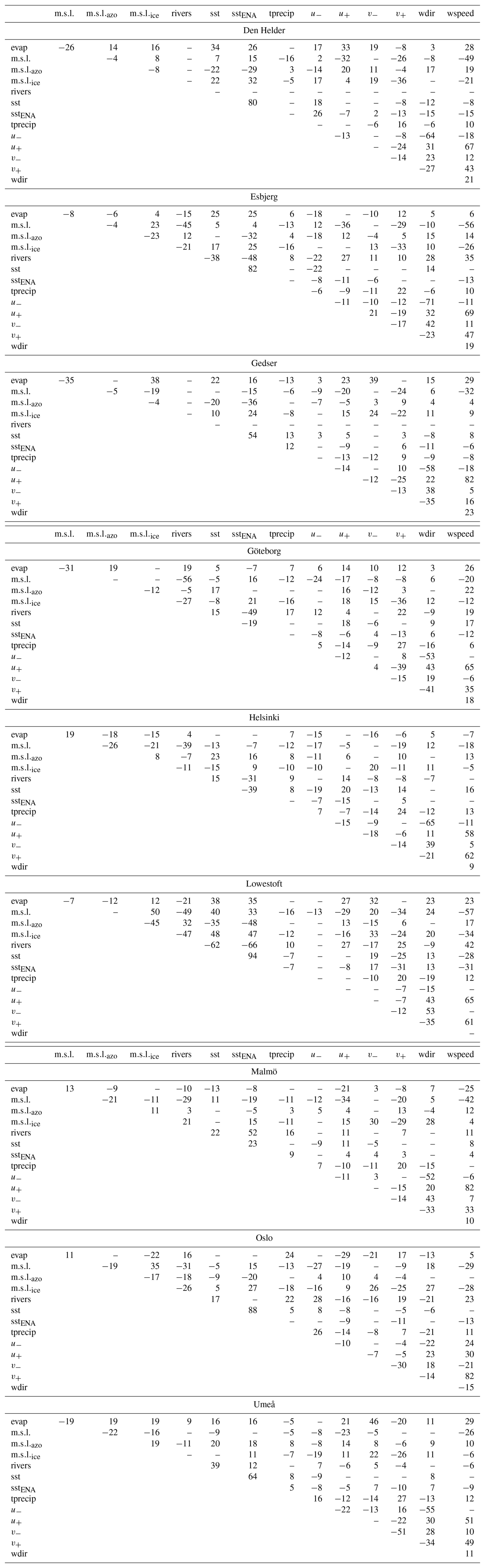
Table A2 For each city and for LSTM, the explained variance (R², %) of the default run with all of the predictors (top row) is shown, together with each run with feature permutation, where the predictor was set to random values.

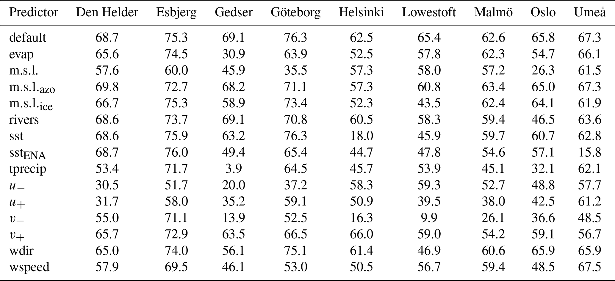
Table A3 Same as Table A2 but for the overall root mean square error.

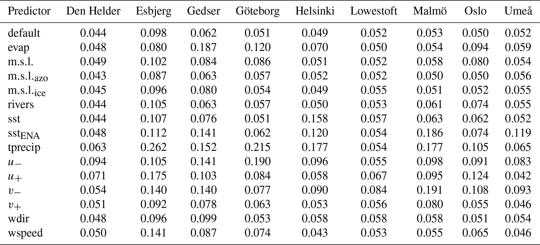
Table A4 Same as Table A2 but for the root mean square error of the normalised sea level values larger than 0.66 (RMSE_0.66).

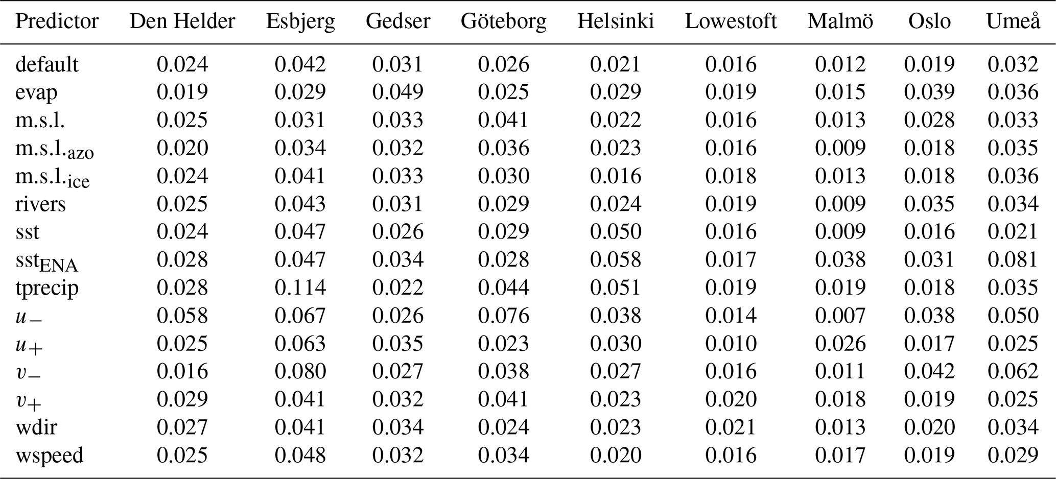
Table A5 For each city and for random forest, the mean performance over 100 runs with all predictors (RMSE, m) and the correlation between the test set and its predicted values are shown.

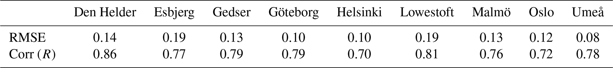
Table A6 For each city and for random forest, the average feature importance and its standard deviation (%) across the 100 ensemble members of the random forest regression are shown for each tested delay (second column) of each predictor (first column). No value means that the feature was never selected as important; see the Methods section.