The alongshore tilt of mean dynamic topography and its implications for model validation and ocean monitoring

Mean dynamic topography (MDT) plays an important role in the dynamics of shelf circulation. Coastal tide gauge observations in combination with the latest generation of geoid models are providing estimates of the alongshore tilt of MDT with unprecedented accuracy. Additionally, high-resolution ocean models are providing better representations of nearshore circulation and the associated tilt of MDT along their coastal boundaries. It has been shown that the newly available geodetic estimates can be used to validate model predictions of coastal MDT variability on global and basin scales. On smaller scales, however, there are significant variations in alongshore MDT that are of the same order of magnitude as the accuracy of the geoid models.

In this study, we use a regional ocean model of the Gulf of Maine and Scotian Shelf (GoMSS) to demonstrate that the new observations of geodetically referenced coastal sea level can also provide valuable information for the validation of such high-resolution models. The predicted coastal MDT is in good agreement with coastal tide gauge observations referenced to the Canadian Gravimetric Geoid 2013 – Version A (CGG2013a), including a significant tilt of alongshore MDT along the coast of Nova Scotia. Using the validated GoMSS model and two idealized models, we show that this alongshore tilt of MDT can be interpreted in two complementary, and dynamically consistent, ways: in the coastal view, the tilt of MDT along the coast can provide a direct estimate of the average alongshore current. In the regional view, the tilt provides a measure of area-integrated nearshore circulation. This highlights the value of using geodetic MDT estimates for model validation and ocean monitoring.

1 Introduction

It has long been recognized that the alongshore tilt of mean dynamic topography (MDT; the local mean sea level above the geoid) plays an important role in the dynamics of shelf circulation (e.g., Scott and Csanady, 1976; Csanady, 1978; Hickey and Pola, 1983; Werner and Hickey, 1983; Lentz, 2008). On the inner shelf (the region just outside the surf zone in water depths of the order of 10 m) frictional effects are dominant. Furthermore, due to the coastal constraint of no normal flow, currents in the nearshore region mostly vary in the alongshore direction (Lentz and Fewings, 2012). It has been shown that this results in continental shelves acting as a low-wavenumber filter (Huthnance, 2004). This implies that mesoscale variations of sea level in the deep ocean are attenuated and only signals with large alongshore length scales of the order of 1000 km can be detected at the coast.

On the shelf, a multitude of drivers including wind stress, input of freshwater by rivers, and tidal rectification contribute to the circulation and thus impact the sea level at the coast (Lentz and Fewings, 2012). It is important to note that the coast acts as a waveguide and the effect of these drivers can be felt long distances “downstream” in the sense of coastally trapped wave propagation (e.g., Csanady, 1978; Thompson, 1986; Thompson and Mitchum, 2014; Frederikse et al., 2017; Hughes et al., 2019; Lentz, 2024). The large number of drivers, and the possibility of remote effects, has resulted in debate about the origin of the observed alongshore pressure gradient at the coast (e.g., Csanady, 1978; Chapman et al., 1986; Xu and Oey, 2011).

MDT appears in the momentum equation in the form of a gradient term and is thus an integrated measure of the mean circulation. This makes MDT a potentially useful variable for ocean monitoring and the validation of ocean models. The direct observation of MDT is complicated by the need to specify the geoid, relative to which MDT is defined. However, recent advances in geodesy have led to new and improved models of the geoid that can be used to get reliable estimates of MDT at coastal tide gauges (Woodworth et al., 2012). In coastal regions with flat topography, these independent measurements are accurate on the centimeter level (Huang, 2017) and thus provide potentially valuable information for the validation of ocean and shelf circulation models.

Higginson et al. (2015) compared multiple global ocean models with geodetically referenced sea level observations along the east coast of North America using different geoid models. While they showed a general convergence between the estimates of MDT, they also pointed out that some models predicted a drop near Cape Hatteras that is not evident in the observations. They concluded that these models did not capture the attenuation of the deep-ocean signal over the shelf. A similar analysis was done by Lin et al. (2015) for the Pacific coasts of North America and Japan. They demonstrated good agreement between the two approaches and furthermore used an analysis of the momentum budget along the coasts to illustrate the dominant dynamics behind the observed MDT. These studies as well as others (e.g., Hughes et al., 2015; Ophaug et al., 2015; Woodworth et al., 2015; Filmer et al., 2018) illustrate the value of the newly available geodetic estimates of coastal MDT for model validation. On the other hand, the overall convergence of the geodetically estimated and predicted MDT simultaneously also increases confidence in the geoid models (Huang, 2017).

Most of the previous studies, including the ones mentioned above, focus on global- and basin-scale variability of MDT at the coast. There are, however, significant variations on smaller scales that are of the same order of magnitude as the accuracy of the geoid models. In this study, we focus on the MDT along the northwest Atlantic coast predicted by the Gulf of Maine and Scotian Shelf (GoMSS) model (Katavouta and Thompson, 2016). The circulation in this region is part of a large-scale buoyancy-driven coastal circulation originating along the south coast of Greenland (Chapman and Beardsley, 1989). On smaller scales, tidal rectification can generate mean currents up to 20 cm s⁻¹ (Loder, 1980), and it has been shown that GoMSS is able to capture these processes well (Katavouta and Thompson, 2016; Katavouta et al., 2016).

This raises the following research questions: can new observations of geodetically referenced coastal sea level help validate high-resolution models? What can the alongshore tilt of MDT at the coast tell us about shelf circulation? What are the implications for coastal monitoring? These questions are of practical importance because (i) MDT provides an integrated measure of the mean circulation, (ii) tide gauges are cheap to deploy and maintain compared to many other oceanographic observing platforms (e.g., ships and gliders), and (iii) long records (several decades of hourly data) exist for some locations, thereby providing a background against which to interpret more recent variability. Using GoMSS and two idealized models, we demonstrate that alongshore MDT can be used to estimate not only flow along the coast, but also diagnostics of area-integrated nearshore circulation.

This study is structured as follows: Sect. 2 provides a description of the approaches to estimate coastal MDT from sea level observations and ocean models. In Sect. 3, the mean circulation and MDT predicted by GoMSS are presented and validated using geodetically referenced sea level measurements by tide gauges. In Sect. 4, two views of the dynamical role of the alongshore tilt of MDT at the coast are introduced and subsequently tested in both idealized models of shelf circulation (Sect. 5) and the realistic GoMSS model (Sect. 6). The results are summarized and implications for ocean monitoring are discussed in Sect. 7.

2 Estimating the alongshore tilt of coastal MDT

Mean dynamic topography (MDT), henceforth denoted by η, refers to the mean sea level (MSL) above the geoid corrected for the inverse barometer effect and averaged over a period of time to remove tidal and meteorological variations. MDT is also referred to as ocean dynamic sea level and is solely defined by ocean dynamics and density (Gregory et al., 2019). The alongshore tilt of MDT can be estimated using two independent approaches: a geodetic approach based on sea level observations and a hydrodynamic approach based on ocean circulation models. In this section, these approaches are outlined and information about data used in this study is presented.

2.1 Geodetic approach

In the geodetic approach, sea level measurements by tide gauges relative to tidal benchmarks are referenced to a common vertical datum, which is traditionally estimated by spirit leveling (Huang, 2017). Recent advances by the geodetic community have led to new and improved high-resolution geoid models with an accuracy of several centimeters. These geoid models provide the geoid height relative to a reference ellipsoid. Through satellite-based navigation systems (e.g., Global Positioning System, GPS), sea level heights measured by tide gauges relative to the same ellipsoid can be determined. Subtracting the local geoid height yields an estimate of the MDT:

$$\begin{array}{}\text{(1)}& \mathit{\eta }={\mathit{\eta }}_{\text{BM}}+h_{\text{e}}-N,\end{array}$$

where η_BM is the MSL relative to the GPS tidal benchmark with height h_e above the reference ellipsoid, and N is the geoid height above the same ellipsoid.

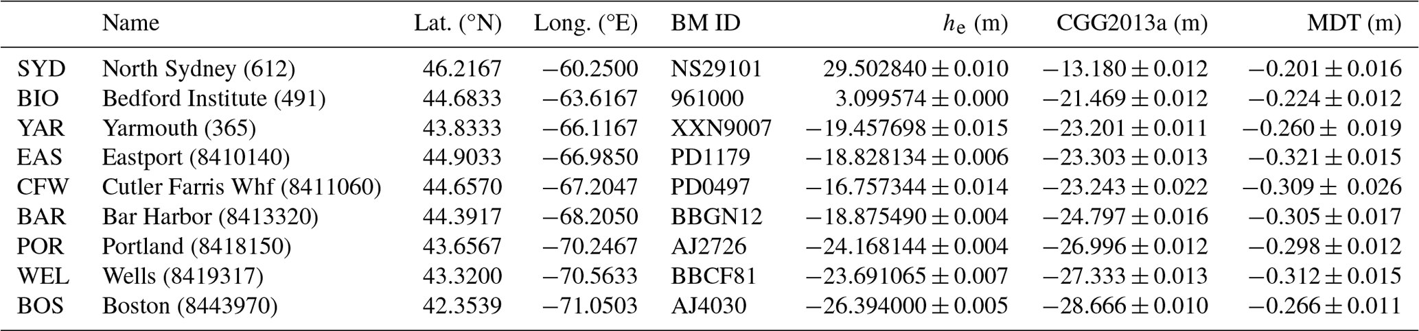
MSL values were computed from hourly observations of sea level at available tide gauges in the Gulf of Maine and Scotian Shelf area for the period 2011–2013. These tide gauges measure the real, observed height of the air–sea interface using acoustic, microwave radar, or air-pressure-compensated pressure sensors. Since the focus of this study is on the regional-scale MDT signal, only tide gauges that are not influenced by highly localized effects were considered (see below). Table 1 gives a summary of the stations used in this study, and their locations are shown in Fig. 1. Overall, the proportion of missing values over the study period is less than 3 % at all stations.

For stations in the USA, hourly water level records with respect to Mean Lower Low Water (MLLW) were retrieved from the National Oceanic and Atmospheric Administration (NOAA). The tide gauge in Chatham, Lydia Cove, MA (NOAA ID 8447435), was excluded because of its location in a shallow lagoon behind a series of sandbars. GPS ellipsoidal heights at nearby benchmarks were obtained from the Online Positioning User Service (OPUS) provided by the National Geodetic Survey (NGS). Their shared solutions list benchmark coordinates relative to the North American Datum, NAD83(2011) epoch 2010.0. They were converted to the International Terrestrial Reference System, ITRF2008 epoch 2010.0 (Altamimi et al., 2011), using the Horizontal Time-Dependent Positioning tool (HTDP; Pearson and Snay, 2013) provided by NGS. At benchmarks where multiple OPUS shared solutions were available, the one with the smallest uncertainty in observed ellipsoidal height was chosen. Using information from benchmark sheets about the relative height of the benchmarks with respect to MLLW, the sea level observations were expressed relative to the GRS80 ellipsoid.

For tide gauges in Canada, hourly water level records with respect to chart datum (CD) were obtained from the Canadian Hydrographic Service (CHS). GPS ellipsoidal heights were obtained for nearby benchmarks of the Natural Resources Canada (NRCAN) High-Precision 3D Geodetic Network in the ITRF2008 epoch 2010.0 reference frame. Generally, the height of the benchmark relative to CD is not known but can be inferred from orthometric height differences with tidal benchmarks of NRCAN's Vertical Passive Control Network published by CHS. Using this information, MSL can be expressed relative to the GRS80 ellipsoid.

Note that the tide gauge for Saint John, NB, Canada (CHS ID 65), was excluded because it is situated in the mouth of St. John River and sheltered by breakwaters. It follows that sea level variations at this tide gauge are likely to be dominated by local processes (e.g., tides and river discharge). The permanent tide gauges located in Halifax, NS, Canada (CHS ID 490), and at the Bedford Institute of Oceanography, Dartmouth, NS, Canada (CHS ID 491), are only a few kilometers apart. Here, the record at the latter will be used because it has fewer missing values and is closer to the GPS benchmark. (The resulting MDTs agree within millimeters.)

The Canadian Gravimetric Geoid 2013 – Version A (CGG2013a; Véronneau and Huang, 2016) was used to provide the geoid height relative to the GRS80 ellipsoid in the ITRF2008 epoch 2010.0 reference frame including a measure of its accuracy. The CGG2013a geoid heights are available on a grid with 2^′ spacing. These were bilinearly interpolated to the benchmark locations and then subtracted from the MSL referenced to the benchmarks.

GPS coordinates are generally expressed in a tide-free coordinate system (Woodworth et al., 2012) as is the geoid model CGG2013a. In order to make geodetically referenced MSL observations comparable to ocean circulation models, mean tidal effects on the coordinate systems have to be considered. Therefore, h_e and N were calculated by converting GPS heights and geoid heights from tide-free to mean tide coordinates using the corrections provided by Ekman (1989). Note that the minus sign error reported by Woodworth et al. (2012) was taken into account.

Geodetic estimates of coastal MDT were then computed using Eq. (1). Uncertainties in the geodetic MDT estimates for the study period arise from errors in the GPS ellipsoidal heights as well as geoid height. These uncertainties are independent and their standard deviations are known. It was therefore possible to use conventional error propagation rules to estimate the standard error of the geodetically determined MDT. The main source of uncertainty is the estimated error in the CGG2013a geoid height, which is generally 1 order of magnitude higher compared to errors in the ellipsoidal heights. Overall, the uncertainties in MDT are typically less than 1.6 cm (Table 1).

Table 1 Summary of geodetic MDT observations in the study area for the period 2011–2013. The numbers in parentheses after the station name are the IDs in the NOAA and CHS databases, respectively. The columns “Lat.” and “Long.” list coordinates of the tide gauges. BM ID refers to the permanent identifiers of the GPS benchmarks assigned by NGS and NRCAN, and the ellipsoidal heights at these benchmarks are listed under h_e. The geoid heights N interpolated to the benchmark locations are listed in column CGG2013a. In the last column, the resulting geodetic estimates of MDT are presented. Their error is a combination of the errors in h_e and N and was calculated using standard error propagation rules.

Since MDT is solely defined by ocean dynamics and density (Gregory et al., 2019), the geodetic MDT estimates were corrected for the inverse barometer effect following Andersen and Scharroo (2011). Here, 6-hourly data of air pressure reduced to MSL from the NCEP Climate Forecast System Version 2 (CFSv2; Saha et al., 2014) were used. The time-mean air pressure p_a at the grid point closest to the tide gauges was used to compute the mean inverse barometer correction in centimeters:

$$\begin{array}{}\text{(2)}& {\mathit{\eta }}_{\text{IB}}={\displaystyle \frac{p_{\text{a}}-p_{\text{ref}}}{{\mathit{\rho }}_{\mathrm{0}}g}}=\mathrm{0.99485}\mathrm{cm}{\mathrm{hPa}}^{-\mathrm{1}}\left(p_{\text{a}}-p_{\text{ref}}\right),\end{array}$$

which was added to the geodetic MDT estimates. Here, p_ref= 1013.0 hPa is the atmospheric reference pressure. The difference in the mean inverse barometer effect between the tide gauges in Boston and North Sydney is 2 cm.

2.2 Hydrodynamic approach

Ocean circulation models typically have their vertical coordinate system expressed relative to an equipotential surface assumed to be the geoid. Therefore, MSL predicted by the model is equal to the MDT (plus an unknown, dynamically irrelevant constant) and can be directly compared to the geodetic estimates. This is referred to as the hydrodynamic or ocean approach (e.g., Woodworth et al., 2012).

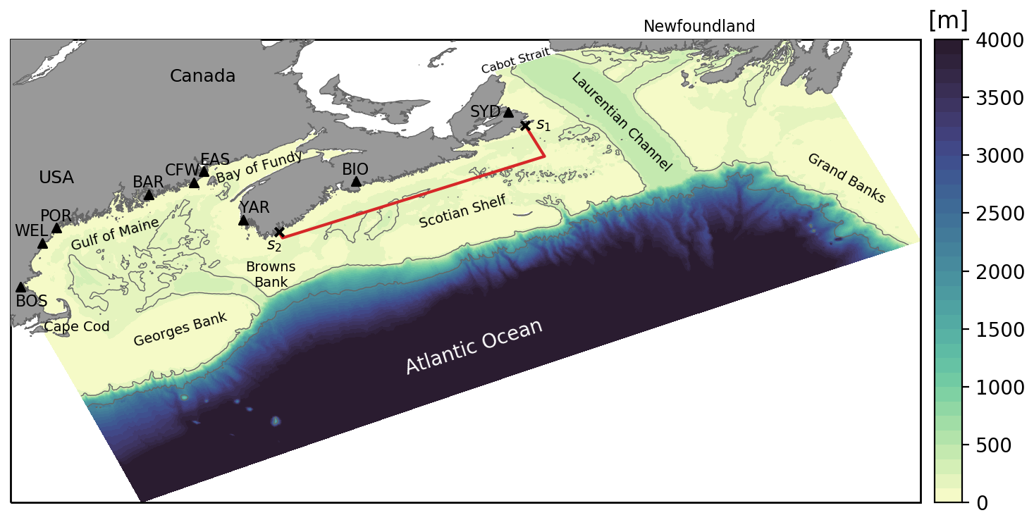
Figure 1 GoMSS model domain and tide gauge locations for the Scotian Shelf, Gulf of Maine, and Bay of Fundy. Contours indicate the 200 and 2000 m isobaths. The triangles indicate the tide gauge locations, with the abbreviations referring to the stations listed in Table 1. The area enclosed by the red polygon and the coastline illustrates the region over which the regional view is evaluated, and the markers s₁ and s₂ indicate reference points along the coast.

To estimate the MDT along the northwest Atlantic coast, we use the Gulf of Maine and Scotian Shelf (GoMSS; Fig. 1) model developed by Katavouta and Thompson (2016) and upgraded by Renkl and Thompson (2022). GoMSS is based on version 3.6 of the Nucleus for European Modelling of the Ocean (NEMO; Madec et al., 2017). In comparison to the original configuration, the bathymetry was replaced with a combination of the 30^′′ GEBCO bathymetry (Weatherall et al., 2015) and high-resolution in situ measurements using an optimal interpolation procedure. This was done to ensure the bathymetry is accurately represented in GoMSS, particularly in shallow regions. GoMSS has a horizontal grid spacing of 1/36°, corresponding to 2.1 to 3.6 km in the study region. The model has 52 vertical z levels that, in a state of rest, increase in thickness from 0.72 m at the surface to 235.33 m at depth but vary in time via a variable volume formulation of the nonlinear free surface (z* coordinate; Levier et al., 2007). Partial cells at the bottom ensure a better resolution of the bathymetry that is clipped at 4000 m.

Both the initial conditions and lateral boundary forcing are based on water temperature, salinity, sea surface height, and currents from the GLORYS12v1 reanalysis (Lellouche et al., 2021). Additionally, tidal elevation and currents for five tidal constituents (M₂, N₂, S₂, K₁, O₁) from FES2004 (Lyard et al., 2006) were prescribed along the lateral boundaries. Atmospheric forcing at the air–sea boundary was based on the CFSv2 (0.5° grid spacing; Saha et al., 2014).

The following analysis is based on daily mean output fields of a hindcast for the period 2011–2013. Note that GoMSS does not include forcing by atmospheric pressure, and therefore no corrections for the inverse barometer effect have to be applied to the model output.

Model predictions of the alongshore MDT from the hydrodynamic approach are based on the predicted MSL over the 3-year period. The coastal MDT is taken at the wet (non-land) grid cell closest to the coast, and the alongshore tilt of MDT, in the following denoted by Δη_c, is the difference in MDT between two points along the coast.

3 Model prediction of mean circulation and validation using geodetically estimated MDT

Before the dynamical role of Δη_c is explored in the realistic, high-resolution regional ocean model GoMSS, its predictions of the MDT and mean circulation are presented. To illustrate the main features of the circulation in the Scotian Shelf and Gulf of Maine region, the mean depth-averaged currents predicted by GoMSS for the period 2011–2013 are shown in Fig. 2.

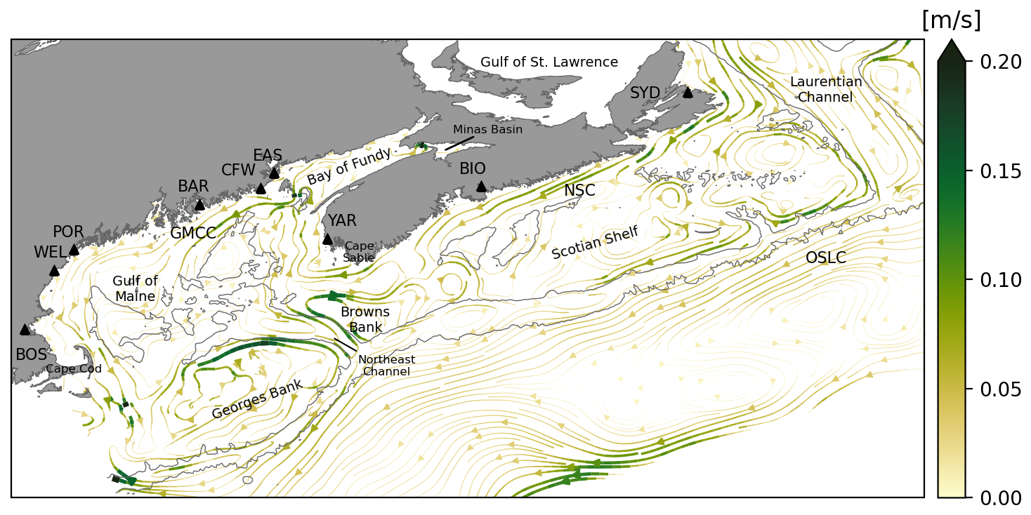
Figure 2 Streamlines of mean depth-averaged circulation predicted by GoMSS for the period 2011–2013. Gray contours mark the 200 and 2000 m isobaths, and triangles show the locations of the tide gauges listed in Table 1. Acronyms indicate circulation features described in the text. NSC: Nova Scotia Current; OSLC: offshore Labrador Current; GMCC: Gulf of Maine Coastal Current.

GoMSS is able to capture the main features of the mean circulation, which are closely connected to the complex bathymetry in the region and have been documented in numerous studies. The nearshore outflow from the Gulf of Saint Lawrence through Cabot Strait is the origin of the Nova Scotia Current (NSC), which follows the coastline toward the Gulf of Maine. This outflow is associated with relatively fresh and cold water originating from the inshore Labrador Current and runoff from the Saint Lawrence River (e.g., Smith and Schwing, 1991; Hannah et al., 2001; Dever et al., 2016; Rutherford and Fennel, 2018). Another part of the outflow through Cabot Strait follows the western side of the Laurentian Channel and joins the offshore branch of the Labrador Current (OSLC) flowing along the shelf break. The strong current along the offshore boundary of GoMSS is related to mesoscale eddies associated with the Gulf Stream outside the model domain and is also present in the forcing data from GLORYS12v1 (not shown).

On the shelf and in the Gulf of Maine, the mean circulation is dominated by rectified tidal flow, which is aligned with bathymetric features. Most notable is the clockwise gyre on Georges Bank with predicted residual currents up to 20 cm s⁻¹ along its northern flank. This is consistent with previous studies and has been attributed to tidal rectification and thermal wind associated with a tidal mixing front (Loder, 1980; Butman et al., 1982; Greenberg, 1983; Naimie et al., 1994; Naimie, 1996; Chen et al., 2001; Brink et al., 2009). GoMSS also predicts a clockwise gyre over Browns Bank, which is caused by the same mechanisms (e.g., Greenberg, 1983; Smith, 1983; Tee et al., 1993; Hannah et al., 2001). These two gyres create an inflow–outflow pattern in the Northeast Channel.

In the vicinity of Cape Sable, strong tidal currents generate a tidally rectified mean flow that locally enhances the Nova Scotia Current. It has been shown that this is also associated with permanent topographic upwelling in that region (Garrett and Loucks, 1976; Greenberg, 1983; Tee et al., 1988, 1993; Chegini et al., 2018).

In the Gulf of Maine, GoMSS predicts a generally counterclockwise circulation. One dominant feature is the Gulf of Maine Coastal Current (GMCC) flowing from the Bay of Fundy along the coast of Maine and splitting into two branches south of Bar Harbor (BAR). This pattern is consistent with observations and is primarily driven by a pressure gradient force (Pettigrew et al., 1998, 2005).

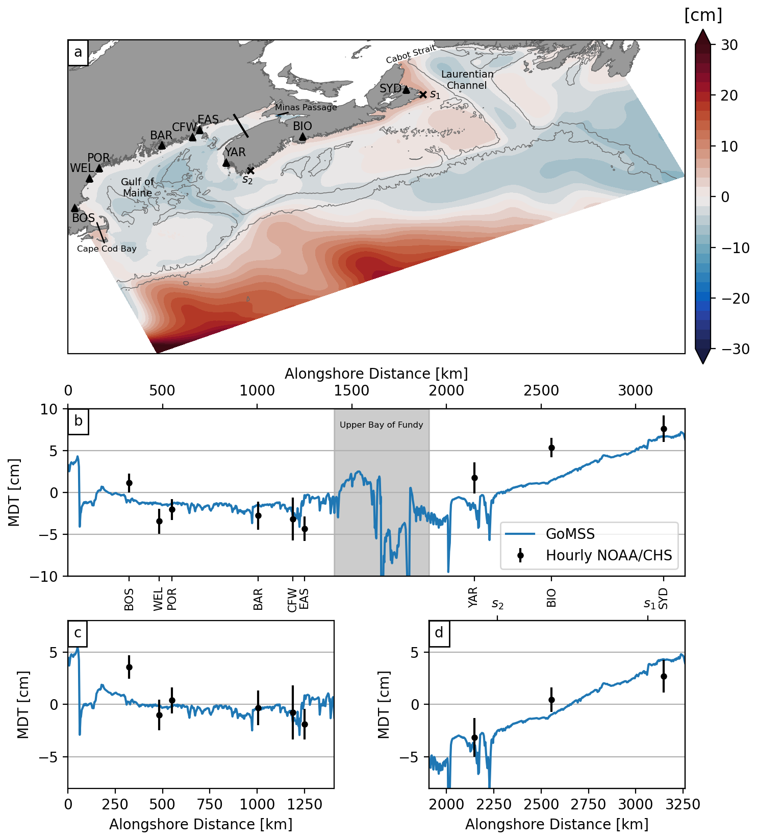
Figure 3 Predicted and observed mean dynamic topography (MDT). (a) MDT predicted by GoMSS (spatial median value over an area where water depth < 200 m is removed). Markers indicate the locations of the coastal tide gauges listed in Table 1. The line separates the upper Bay of Fundy where the model has difficulty resolving the residual circulation due to the limited resolution. (b) Coastal MDT as a function of distance along the coast of the Gulf of Maine and Nova Scotia. The minima in Minas Passage (−28 and −25 cm, respectively) are not shown. Geodetic estimates of MDT are shown with their respective uncertainty. The shaded area indicates the coast along the upper Bay of Fundy. Panels (c) and (d) show enlarged views of either side of the shaded area in (b). In panels (b)–(d), the means of the respective observations and predictions at the grid points closest to the tide gauges have been removed.

The circulation features described above are also expressed in the MDT predicted by GoMSS (Fig. 3a). To center MDT variations on the shelf (water depths < 200 m) around zero, the spatial median value over this region has been subtracted. Contours indicate the 200 and 2000 m isobaths, which mark the shelf break as well as important banks and channels on the shelf. Triangles show the locations of the tide gauges listed in Table 1.

The strong signal in the deep ocean is related to eddies associated with the Gulf Stream and the offshore branch of the Labrador Current. On the shelves, variations in MDT are generally aligned with bathymetric features, which is consistent with the topographically driven and tidally rectified circulation described above.

Relatively high values of MDT are predicted on the western side of Cabot Strait associated with the outflow from the Gulf of Saint Lawrence. The offshore gradient of MDT suggests a geostrophic balance with the Nova Scotia Current. Additionally, areas of elevated MDT are apparent over the banks on the shelf driven by tidal rectification. In the Gulf of Maine, MDT is generally lower toward the center, which is consistent with the overall counterclockwise circulation. This is also in agreement with observations (Li et al., 2014a). As shown by Renkl and Thompson (2022), the predicted MDT in the upper Bay of Fundy has to be treated with caution because of the limited spatial resolution of GoMSS in that region.

3.1 Model validation using geodetic tilt estimates

In Fig. 3b, the predicted and observed MDTs along the coast are shown as a function of alongshore distance from Cape Cod to Cabot Strait. The means of the observations and predictions of coastal MDT at the grid points closest to the tide gauges have been removed.

The shaded area marks the coastline in the upper Bay of Fundy and more clearly illustrates the strong set-down in that area. As discussed above, the MDT prediction in that region has to be treated with caution, and therefore the coastline is separated into two parts along the Gulf of Maine (Fig. 3c) and Nova Scotia (Fig. 3d), respectively. In both panels, the means of the respective observations and predictions at the grid points closest to the tide gauges have been removed.

Along the coast of the Gulf of Maine, the predicted coastal MDT is mostly flat, with a small increase toward Cape Cod Bay due to wind setup (not shown). The small-scale variability originates from local interactions between the flow and bathymetry in tidal inlets, which are part of the rugged coastline. While the predicted local minimum near Cutler Farris Wharf (CFW) and Eastport (EAS) is due to local processes, the overall difference in MDT either side of this set-down is presumably associated with the Gulf of Maine Coastal Current.

The alongshore MDT predicted along the coast of the Gulf of Maine agrees well with the geodetic estimates. The largest discrepancy is found at Boston (BOS) where the tide gauge is located inside the harbor, sheltered from the open ocean. Therefore, it is likely that the strong setup seen in the observations is a manifestation of local processes. However, it cannot be ruled out that the wind setup toward Cape Cod Bay is underestimated in GoMSS.

Along the coast of Nova Scotia (Fig. 3d), both the observations and predictions show a strong tilt of coastal MDT. The observed difference in MDT between the tide gauges in Sydney (SYD) and Yarmouth (YAR) is Δη_c= 5.9±2.0 cm. GoMSS predicts a tilt of Δη_c= 8.3 cm. This is slightly larger than the geodetically estimated tilt but within 2 standard deviations of the observed value. Note that a local set-down near YAR is predicted, which is related to strong tidal currents in that region. The tide gauge itself is located inside Yarmouth Harbour, which is not resolved in the model. This will lead to discrepancies between the model and observations.

Rather than stating Δη_c as a difference between two fixed locations, it is often reported as the alongshore gradient consistent with its expression in the momentum equation. However, it is not straightforward to calculate the coastal MDT gradient because the irregular shape of the coastline leads to uncertainty in the distance between the fixed locations (Mandelbrot, 1982). For example, using an alongshore distance of ΔL= 999 km computed from the coastline in GoMSS results in a predicted MDT gradient of $\mathrm{\Delta }{\mathit{\eta }}_{\text{c}}/\mathrm{\Delta }L=$ $\mathrm{8.4}\times {\mathrm{10}}^{-\mathrm{8}}$ (equivalent to 0.8 cm per 100 km). If the interest is the large-scale gradient, this value is arguably an underestimation. If instead one were to use ΔL= 650 km based on three straight line segments from SYD to YAR, the gradient is $\mathrm{\Delta }{\mathit{\eta }}_{\text{c}}/\mathrm{\Delta }L=$ $\mathrm{1.3}\times {\mathrm{10}}^{-\mathrm{7}}$. This gradient is comparable to the values used by Smith (1983) in his diagnostic model to describe the circulation off southwest Nova Scotia. However, the above discussion highlights the subjectivity that can be introduced by focusing on gradients rather than Δη_c between two fixed locations.

In addition to the large-scale tilt, GoMSS predicts local minima of MDT around YAR and just southeast of it at Cape Sable. As discussed above in relation to the mean circulation, these set-downs can be explained by the strong tidal currents and the curvature of the coastline in that region (e.g., Greenberg, 1983; Smith, 1983; Tee et al., 1993; Chegini et al., 2018).

The above discussion answers the first major question raised in the Introduction: can new observations of geodetically referenced coastal sea level help validate high-resolution regional ocean models? The overall agreement of Δη_c estimated independently by the hydrodynamic and geodetic approaches provides validation of the ocean model. This gives confidence that GoMSS captures the mean shelf-scale ocean circulation on the Scotian Shelf and in the Gulf of Maine. While there are some limitations to this method (see Sect. 7), the dynamical interpretation of Δη_c below illustrates that the alongshore tilt of MDT is an integrated measure of nearshore ocean dynamics, highlighting its usefulness for model validation. Specifically, the next sections address the following questions: what can the alongshore tilt of MDT at the coast tell us about shelf circulation? What are the implications for coastal monitoring?

4 Dynamical interpretation of Δη_c

Assuming steady state and neglecting the inverse barometer effect, the linearized momentum equation for the depth-averaged current $\stackrel{\mathrm{‾}}{\mathit{u}}$ can be written as

$$\begin{array}{}\text{(3)}& g\mathrm{\nabla }\left(\mathit{\eta }-{\mathit{\eta }}_{\text{s}}\right)=-f\widehat{\mathit{k}}\times \stackrel{\mathrm{‾}}{\mathit{u}}-{\displaystyle \frac{\mathrm{1}}{H}}\mathrm{\nabla }\mathit{\chi }+{\displaystyle \frac{{\mathit{\tau }}^{\text{w}}-{\mathit{\tau }}^{\text{b}}}{{\mathit{\rho }}_{\mathrm{0}}H}}+{\stackrel{\mathrm{‾}}{\mathit{D}}}_{\text{l}},\end{array}$$

which is a slightly rewritten form of the one presented by Csanady (1979) to include effects of lateral friction and separate the baroclinic pressure into the steric contribution to the sea level,

$$\begin{array}{}\text{(4)}& {\mathit{\eta }}_s=-\underset{-H}{\overset{\mathrm{0}}{\int }}\mathit{ϵ}\mathrm{d}z,\end{array}$$

and the vertically integrated potential energy anomaly,

$$\begin{array}{}\text{(5)}& \mathit{\chi }=g\underset{-H}{\overset{\mathrm{0}}{\int }}z\mathit{ϵ}\mathrm{d}z.\end{array}$$

Here, $\mathit{ϵ}=(\mathit{\rho }-{\mathit{\rho }}_{\mathrm{0}})/{\mathit{\rho }}_{\mathrm{0}}$ is the normalized density perturbation and H is the water depth at rest. Equation (3) can be considered an equation for the gradient of the dynamically active component of sea level, multiplied by the vertical acceleration due to gravity g, that is balanced by the Coriolis term with parameter f, the gradient of χ, the difference between wind stress (τ^w) and bottom stress (τ^b), and lateral friction (${\stackrel{\mathrm{‾}}{\mathit{D}}}_{\text{l}}$).

Taking the curl of Eq. (3) and neglecting latitudinal variations of the Coriolis parameter leads to the following equation for the vorticity of the depth-averaged flow on an f plane (e.g., Mertz and Wright, 1992):

$$\begin{array}{}\text{(6)}& \begin{array}{rl}-{\displaystyle \frac{f}{H}}\stackrel{\mathrm{‾}}{\mathit{u}}& \cdot \mathrm{\nabla }H=J\left(\mathit{\chi },H^{-\mathrm{1}}\right)+\widehat{\mathit{k}}\cdot \mathrm{\nabla }\times \left({\displaystyle \frac{{\mathit{\tau }}^{\text{w}}-{\mathit{\tau }}^{\text{b}}}{{\mathit{\rho }}_{\mathrm{0}}H}}\right)\\ & +\widehat{\mathit{k}}\cdot \mathrm{\nabla }\times {\stackrel{\mathrm{‾}}{\mathit{D}}}_{\text{l}},\end{array}\end{array}$$

describing the change in potential vorticity due to vortex tube stretching by flow across isobaths.

The first term on the right-hand side of Eq. (6) is the joint effect of baroclinicity and relief (JEBAR; Sarkisyan and Ivanov, 1971):

$$\begin{array}{}\text{(7)}& J\left(\mathit{\chi },H^{-\mathrm{1}}\right)={\displaystyle \frac{\partial \mathit{\chi }}{\partial x}}{\displaystyle \frac{\partial H^{-\mathrm{1}}}{\partial y}}-{\displaystyle \frac{\partial \mathit{\chi }}{\partial y}}{\displaystyle \frac{\partial H^{-\mathrm{1}}}{\partial x}}.\end{array}$$

As shown by Mertz and Wright (1992), this can be interpreted as the baroclinic contribution to the torque related to the depth-averaged pressure. They furthermore showed that JEBAR acts as a correction to the vortex stretching term in Eq. (6) by removing the nonphysical contribution of the geostrophic flow referenced to the bottom. Note that JEBAR vanishes in the case of constant water depth. The remaining terms in Eq. (6) describe the curl of the difference between wind stress and bottom friction and their associated Ekman transports across depth contours, as well as the effects of lateral friction.

In the following, Eqs. (3) and (6) will be used to explore the role of Δη_c in coastal and shelf circulation.

4.1 Interpretation of Δη_c in terms of coastal circulation

At the coast, the depth-averaged momentum balance (Eq. 3) simplifies. Due to the condition of no flow across the coastal boundary, the first term on the right-hand side vanishes in the alongshore component. Furthermore, it is assumed that density variations along the coast, i.e., the combined effect of ∇η_s and $\frac{\mathrm{1}}{H}\mathrm{\nabla }\mathit{\chi }$, can be neglected. This assumption will be shown to be reasonable in the analysis of the alongshore momentum balance predicted by GoMSS in Sect. 6.1. It follows from Eq. (3), under the assumption of steady state, that the momentum equation in the alongshore direction reduces to

$$\begin{array}{}\text{(8)}& g\mathrm{\nabla }\mathit{\eta }={\displaystyle \frac{{\mathit{\tau }}^{\text{w}}-{\mathit{\tau }}^{\text{b}}}{{\mathit{\rho }}_{\mathrm{0}}H}}+{\stackrel{\mathrm{‾}}{\mathit{D}}}_{\text{l}}.\end{array}$$

Thus, the large-scale alongshore gradient of MDT at the coast is primarily balanced by the sum of wind stress, bottom drag, and horizontal mixing.

The integral of Eq. (8) along a curve C_c following the coastline between two points (see Fig. 4) gives the large-scale alongshore balance of the tilt of MDT in vector form:

$$\begin{array}{}\text{(9)}& g\mathrm{\Delta }{\mathit{\eta }}_{\text{c}}=\underset{C_{\text{c}}}{\int }\left[{\displaystyle \frac{{\mathit{\tau }}^{\text{w}}-{\mathit{\tau }}^{\text{b}}}{{\mathit{\rho }}_{\mathrm{0}}H}}+{\stackrel{\mathrm{‾}}{\mathit{D}}}_{\text{l}}\right]\cdot \mathrm{d}\mathit{r},\end{array}$$

where dr is the unit vector parallel to the integration path. This is one interpretation of Δη_c in terms of coastal circulation. From Eq. (9) it is clear that, along the coast, the tilt of MDT is in frictional equilibrium. In the following, this interpretation is referred to as the coastal view.

In the special case when the sea level difference along the coast due to wind stress,

$$\begin{array}{}\text{(10)}& g\mathrm{\Delta }{\mathit{\eta }}_{\text{w}}=\underset{C_{\text{c}}}{\int }{\displaystyle \frac{{\mathit{\tau }}^{\text{w}}}{{\mathit{\rho }}_{\mathrm{0}}H}}\cdot \mathrm{d}\mathit{r},\end{array}$$

is known, a new variable $\stackrel{\mathrm{̃}}{\mathit{\eta }}$ can be defined as the wind-corrected MDT. More generally, it can be shown that $\stackrel{\mathrm{̃}}{\mathit{\eta }}$ could also incorporate corrections for the neglected nonlinear terms (e.g., the Bernoulli effect) and atmospheric pressure variations. Thus, Eq. (9) becomes

$$\begin{array}{}\text{(11)}& g\mathrm{\Delta }{\stackrel{\mathrm{̃}}{\mathit{\eta }}}_{\text{c}}=-\underset{C_{\text{c}}}{\int }\left[{\displaystyle \frac{{\mathit{\tau }}^{\text{b}}}{{\mathit{\rho }}_{\mathrm{0}}H}}-{\stackrel{\mathrm{‾}}{\mathit{D}}}_{\text{l}}\right]\cdot \mathrm{d}\mathit{r}.\end{array}$$

If τ^b is parameterized in terms of the depth-averaged current, ${\stackrel{\mathrm{‾}}{\mathit{D}}}_{\text{l}}$ can be neglected (e.g., outside a narrow viscous boundary layer), and the wind-driven tilt along the coast is known, it will be shown that $\mathrm{\Delta }{\stackrel{\mathrm{̃}}{\mathit{\eta }}}_{\text{c}}$ can be interpreted as a measure of the average alongshore flow between two points along the coast.

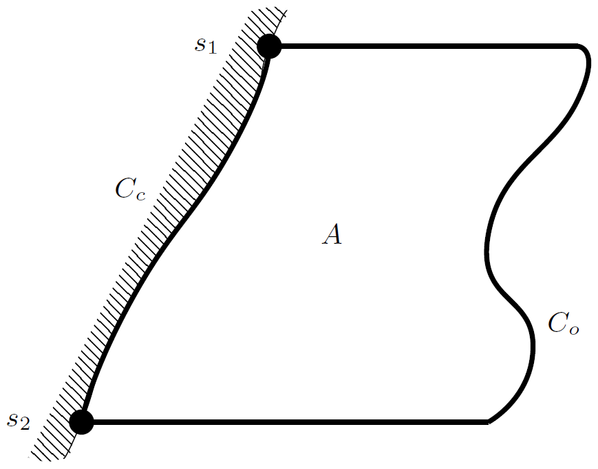
Figure 4 Schematic of a closed curve along which the momentum balance is integrated. The hatched area is the land, and the bold line illustrates the closed integration path C, which can be divided into a coastal (C_c) and offshore part (C_o). The area enclosed by C is denoted by A.

4.2 Interpretation of Δη_c in terms of regional circulation

Instead of integrating the momentum balance along the coast, it is also possible to define an offshore curve C_o from s₂ to s₁ along which Eq. (3) can be integrated. Together with the coastal integration path, this forms a closed curve $C=C_{\text{c}}+C_{\text{o}}$ (Fig. 4). Note that the closed-line integral of the sea level gradient term along C is zero, so

$$\begin{array}{}\text{(12)}& \underset{C_{\text{c}}}{\int }\mathrm{\nabla }\mathit{\eta }\cdot d\mathit{r}+\underset{C_{\text{o}}}{\int }\mathrm{\nabla }\mathit{\eta }\cdot d\mathit{r}=\mathrm{0}.\end{array}$$

This demonstrates that the tilt of MDT along the coast Δη_c must equal the drop along the offshore integration path Δη_o:

$$\mathrm{\Delta }{\mathit{\eta }}_{\text{c}}=-\mathrm{\Delta }{\mathit{\eta }}_{\text{o}}.$$

Since Δη_o is determined by the regional ocean dynamics, it follows that Δη_c can also be interpreted in terms of the regional ocean dynamics.

Using Green's theorem (Green, 1828), the line integral of a two-dimensional vector field F along a closed curve C is equal to the surface integral of the curl of the field over the enclosed area A,

$$\begin{array}{}\text{(13)}& \underset{C}{\oint }\mathit{F}\cdot d\mathit{r}=\underset{A}{\iint }\left(\mathrm{\nabla }\times \mathit{F}\right)\cdot \widehat{\mathit{n}}\mathrm{d}A,\end{array}$$

where $\widehat{\mathit{n}}$ is the unit vector perpendicular to the surface A.

For the case of depth-averaged ocean circulation, the term under the area integral is the relative vorticity of the flow field. Therefore, the circuit integral of the momentum equation is equal to the area integral of the vorticity equation. Combining Eqs. (3) and (13) with the vorticity equation (Eq. 6) gives

$$\begin{array}{}\text{(14)}& \begin{array}{rl}\underset{C}{\oint }& \left[{\displaystyle \frac{{\mathit{\tau }}^{\text{w}}-{\mathit{\tau }}^{\text{b}}}{{\mathit{\rho }}_{\mathrm{0}}H}}+{\stackrel{\mathrm{‾}}{\mathit{D}}}_{\text{l}}\right]\cdot \mathrm{d}\mathit{r}\\ & =\underset{A}{\iint }\left[-{\displaystyle \frac{f}{H}}\stackrel{\mathrm{‾}}{\mathit{u}}\cdot \mathrm{\nabla }H-J\left(\mathit{\chi },H^{-\mathrm{1}}\right)\right]\mathrm{d}A.\end{array}\end{array}$$

The left-hand side is the closed-line integral of the frictional terms, which is balanced by the area integral of vortex tube stretching by flow across isobaths and the JEBAR term. Note that all the gradient terms, including the sea level gradient, have dropped out.

The circuit integral on the left-hand side can be split into a coastal and offshore part. Note that the line integral along the coast is equal to gΔη_c. Hence, substituting Eq. (9) in Eq. (14) gives

$$\begin{array}{}\text{(15)}& \begin{array}{rl}& g\mathrm{\Delta }{\mathit{\eta }}_{\text{c}}=\underset{A}{\iint }\left[-{\displaystyle \frac{f}{H}}\stackrel{\mathrm{‾}}{\mathit{u}}\cdot \mathrm{\nabla }H-J\left(\mathit{\chi },H^{-\mathrm{1}}\right)\right]\mathrm{d}A\\ & -\underset{C_{\text{o}}}{\int }\left[{\displaystyle \frac{{\mathit{\tau }}^{\text{w}}-{\mathit{\tau }}^{\text{b}}}{{\mathit{\rho }}_{\mathrm{0}}H}}+{\stackrel{\mathrm{‾}}{\mathit{D}}}_{\text{l}}\right]\cdot \mathrm{d}\mathit{r},\end{array}\end{array}$$

where the second term on the right-hand side is the offshore segment of the circuit integral in Eq. (14). This is another interpretation of Δη_c, this time in terms of regional ocean dynamics. It shows that the alongshore tilt of MDT at the coast can also be interpreted as an integrated measure of the nearshore ocean circulation. In the following this interpretation will be referred to as the regional view.

Both the coastal and regional views of Δη_c are complementary and dynamically consistent: the offshore circulation drives the coastal dynamics, and, on the other hand, the dynamics along the coast act as a boundary condition for the offshore circulation.

Now consider the JEBAR term, $J\left(\mathit{\chi },H^{-\mathrm{1}}\right)$. Mertz and Wright (1992) showed

$$\begin{array}{}\text{(16)}& J(\mathit{\chi },H^{-\mathrm{1}})=-{\displaystyle \frac{f}{H}}({\stackrel{\mathrm{‾}}{\mathit{u}}}_{\text{g}}-{\mathit{u}}_{\text{g,b}})\cdot \mathrm{\nabla }H,\end{array}$$

where u_g(z) is a geostrophically balanced horizontal velocity defined in terms of the density field according to the following thermal wind equation:

$$\begin{array}{}\text{(17)}& f\widehat{\mathit{k}}\times {\displaystyle \frac{\partial {\mathit{u}}_{\text{g}}}{\partial z}}=g\mathrm{\nabla }\mathit{ϵ},\end{array}$$

with the bottom boundary condition ${\mathit{u}}_{\text{g}}(-H)={\mathit{u}}_{\text{g,b}}$. Mertz and Wright (1992) used Eq. (16) to show that the JEBAR term “represents precisely the geostrophic component of the correction to the topographic stretching term to account for the fact that the bottom velocity, not the depth-averaged velocity, yields topographic vortex-tube stretching”.

Using Eq. (16), the term under the area integral in Eq. (15) can be written as

$$\begin{array}{}\text{(18)}& -{\displaystyle \frac{f}{H}}\stackrel{\mathrm{‾}}{\mathit{u}}\cdot \mathrm{\nabla }H-J\left(\mathit{\chi },H^{-\mathrm{1}}\right)=-{\displaystyle \frac{f}{H}}{\mathit{u}}^{*}\cdot \mathrm{\nabla }H,\end{array}$$

where

$$\begin{array}{}\text{(19)}& {\mathit{u}}^{*}=\stackrel{\mathrm{‾}}{\mathit{u}}-{\stackrel{\mathrm{‾}}{\mathit{u}}}_{\text{g}}+{\mathit{u}}_{\text{g,b}}\end{array}$$

is the total flow minus the geostrophic flow relative to that at the bottom. Hence, the regional view expressed by Eq. (15) can be written as

$$\begin{array}{}\text{(20)}& g\mathrm{\Delta }{\mathit{\eta }}_{\text{c}}=-f\underset{A}{\iint }{\displaystyle \frac{{\mathit{u}}^{*}}{H}}\cdot \mathrm{\nabla }H\mathrm{d}A-\underset{C_{\text{o}}}{\int }\left[{\displaystyle \frac{{\mathit{\tau }}^{\text{w}}-{\mathit{\tau }}^{\text{b}}}{{\mathit{\rho }}_{\mathrm{0}}H}}+{\stackrel{\mathrm{‾}}{\mathit{D}}}_{\text{l}}\right]\cdot \mathrm{d}\mathit{r}.\end{array}$$

In the following sections, we further discuss the coastal and regional views of Δη_c in the context of idealized models for shelf circulation and finally demonstrate that these interpretations also hold in the realistic, high-resolution model GoMSS. Overall, these sections serve to illustrate the versatility of the dynamical interpretations that further highlights the usefulness of the tilt of MDT for ocean model validation and monitoring.

5 Δη_c in idealized ocean models of shelf circulation

The role of the alongshore tilt of MDT in the circulation on continental shelves can be illustrated with the conceptual models discussed by Csanady (1982) that focus on flow trapped within the coastal boundary layer. Consider a coordinate system where the y axis is aligned with a straight coastline and the x axis points offshore. Without lateral mixing and assuming the flow to be steady, linear, and barotropic, the governing equation (Eq. 3) can then be written in component form as

$$\begin{array}{}\text{(21)}& {\displaystyle }g{\displaystyle \frac{\partial \mathit{\eta }}{\partial x}}& {\displaystyle }={\displaystyle \frac{f}{H}}V+{\displaystyle \frac{{\mathit{\tau }}_x^{\text{w}}}{{\mathit{\rho }}_{\mathrm{0}}H}},\text{(22)}& {\displaystyle }g{\displaystyle \frac{\partial \mathit{\eta }}{\partial y}}& {\displaystyle }=-{\displaystyle \frac{f}{H}}U+{\displaystyle \frac{{\mathit{\tau }}_y^{\text{w}}-{\mathit{\tau }}_y^{\text{b}}}{{\mathit{\rho }}_{\mathrm{0}}H}},\end{array}$$

where U and V are the x and y components of the transport vector $\mathit{U}=\stackrel{\mathrm{‾}}{\mathit{u}}H$. The Coriolis parameter f is assumed to be constant. Under the longwave approximation that the alongshore current is much larger than the cross-shore current, the bottom friction in the x direction can be neglected.

Cross-differentiating Eqs. (21) and (22) yields the vorticity equation of this model:

$$\begin{array}{}\text{(23)}& f{\displaystyle \frac{\stackrel{\mathrm{‾}}{u}}{H}}{\displaystyle \frac{\partial H}{\partial x}}=-{\displaystyle \frac{\partial }{\partial x}}\left({\displaystyle \frac{{\mathit{\tau }}_y^{\text{w}}}{{\mathit{\rho }}_{\mathrm{0}}H}}\right)+{\displaystyle \frac{\partial }{\partial y}}\left({\displaystyle \frac{{\mathit{\tau }}_x^{\text{w}}}{{\mathit{\rho }}_{\mathrm{0}}H}}\right)+{\displaystyle \frac{\partial }{\partial x}}\left({\displaystyle \frac{{\mathit{\tau }}_y^{\text{b}}}{{\mathit{\rho }}_{\mathrm{0}}H}}\right).\end{array}$$

The combination of the net torque exerted by the wind stress and bottom drag and their associated Ekman transports across depth contours (right-hand side) is balanced by vortex stretching and squashing through movement into deeper or shallower water, respectively. This flow across isobaths results in convergence or divergence near the seafloor associated with bottom-stress-induced Ekman pumping.

Equation (22) can be rearranged to get an expression for $\stackrel{\mathrm{‾}}{u}$ which can be substituted in Eq. (23). Parameterizing bottom friction with the alongshore geostrophic current times a drag coefficient λ yields a single governing equation for the sea level:

$$\begin{array}{}\text{(24)}& {\displaystyle \frac{{\partial }^{\mathrm{2}}\mathit{\eta }}{\partial x^{\mathrm{2}}}}+{\displaystyle \frac{{\mathit{\rho }}_{\mathrm{0}}f}{\mathit{\lambda }}}{\displaystyle \frac{\partial H}{\partial x}}{\displaystyle \frac{\partial \mathit{\eta }}{\partial y}}={\displaystyle \frac{f}{g\mathit{\lambda }}}\left({\displaystyle \frac{\partial {\mathit{\tau }}_y^{\text{w}}}{\partial x}}-{\displaystyle \frac{\partial {\mathit{\tau }}_x^{\text{w}}}{\partial y}}\right).\end{array}$$

Csanady (1982) pointed out the similarity of Eq. (24) to the heat conduction equation with downstream direction −y corresponding to time. He furthermore used this analogy to discuss coastally trapped flow fields with respect to different forcing. In the following, two cases will be explored and the role of Δη_c discussed.

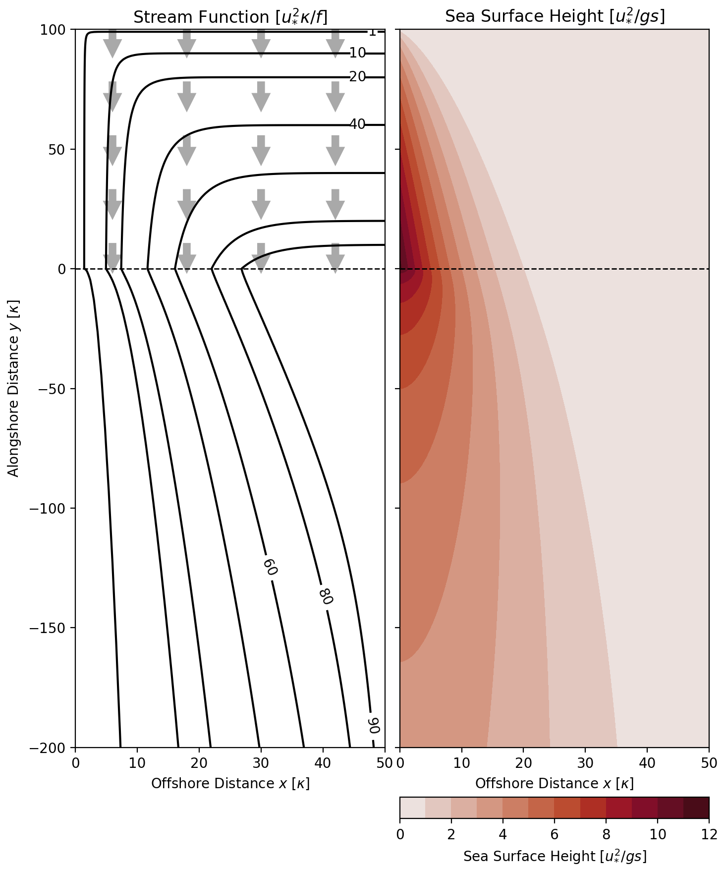
Figure 5 Stream function and sea surface height for two models of coastally trapped circulation. Water depth is increasing in the x direction as $H\left(x\right)=H_{\mathrm{0}}+sx$, the bottom friction coefficient is λ= $\mathrm{0.5}\times {\mathrm{10}}^{-\mathrm{3}}\mathrm{m}{\mathrm{s}}^{-\mathrm{1}}$, and the Coriolis parameter is f= ${\mathrm{10}}^{-\mathrm{4}}{\mathrm{s}}^{-\mathrm{1}}$. For y>0, a spatially uniform wind stress ${\mathit{\tau }}_y^{\text{w}}/{\mathit{\rho }}_{\mathrm{0}}=u_{*}^{\mathrm{2}}=$ $-\mathrm{0.01}{\mathrm{m}}^{\mathrm{2}}{\mathrm{s}}^{-\mathrm{2}}$ (gray arrows) is applied (adapted from Csanady, 1982).

5.1 Wind stress along a portion of the coast

Assume water depth increases linearly with distance from the shore as $H\left(x\right)=H_{\mathrm{0}}+sx$, where s is a constant slope. The wind stress along the part of the domain where $\mathrm{0}\le y\le Y$ is taken to be constant and in the alongshore direction only, ${\mathit{\tau }}^{\text{w}}=(\mathrm{0},{\mathit{\tau }}_y^{\text{w}})$.

As shown above the dashed line in Fig. 5, this wind stress causes an Ekman transport toward the coast if ${\mathit{\tau }}_y^{\text{w}}<\mathrm{0}$. From Eq. (23) it can be seen that the wind stress over the sloping shelf and the flow across isobaths into shallower water exert a negative torque on the water column. Thus, the flow is steered to the left, resulting in an alongshore current at the coast in the direction of the wind. Consequently, sea level piles up in the downstream direction.

Applying the assumptions above to Eq. (9), the coastal view of Δη_c becomes

$$\begin{array}{}\text{(25)}& \mathrm{\Delta }{\mathit{\eta }}_{\text{c}}={\displaystyle \frac{{\mathit{\tau }}_y^{\text{w}}Y}{g{\mathit{\rho }}_{\mathrm{0}}{H}_{\mathrm{0}}}}-{\displaystyle \frac{\mathit{\lambda }}{g{H}_{\mathrm{0}}}}\underset{\mathrm{0}}{\overset{Y}{\int }}\stackrel{\mathrm{‾}}{v}(\mathrm{0},y)\mathrm{d}y.\end{array}$$

The first term on the right-hand side is the wind-driven tilt along the coast. As expected, Δη_c is in frictional equilibrium and balances the difference between wind stress and bottom drag. If the wind setup along the coast is known, the corrected tilt of MDT along the coast $\mathrm{\Delta }{\stackrel{\mathrm{̃}}{\mathit{\eta }}}_{\text{c}}$ can be used as a direct measure of the mean alongshore current.

The regional view can be directly obtained from Eq. (20) under the assumption of barotropic flow, which implies ${\mathit{u}}^{*}=\stackrel{\mathrm{‾}}{\mathit{u}}$. If the offshore integration path is chosen to be in deep water where the wind stress and bottom friction terms are negligible due to their inverse dependence on H, Eq. (20) becomes

$$\begin{array}{}\text{(26)}& \mathrm{\Delta }{\mathit{\eta }}_{\text{c}}=-{\displaystyle \frac{fs}{g}}\underset{\mathrm{0}}{\overset{Y}{\int }}\underset{\mathrm{0}}{\overset{L_x}{\int }}{\displaystyle \frac{\stackrel{\mathrm{‾}}{u}}{H}}\mathrm{d}x\mathrm{d}y.\end{array}$$

This shows that, from a regional perspective, Δη_c is proportional to the cross-shore Ekman transport due to the wind forcing and the associated flow across isobaths. The onshore wind-driven Ekman transport implies downwelling at the coast that is balanced partially by a return flow in the frictional bottom boundary layer and partially by an offshore geostrophic flow in the interior. The total onshore flow is balanced by a divergence of the alongshore flow. The rate of water exchange between the surface Ekman layer and the interior of the water column in that area can be monitored by observing the sea level at the coast.

5.2 Coastal mound

Assume that the wind stress vanishes for y<0 and the flow field is established by prescribing a cross-shore sea level distribution η=η₀(x) at y=0, which is the result of some upstream process, e.g., wind-driven onshore transport as discussed above. It can be seen from Eq. (21) that the corresponding alongshore current is in geostrophic balance.

Figure 5 shows the resulting stream function and the associated sea surface height. The streamlines indicate a predominantly alongshore flow, but they also show a spreading in the offshore direction farther downstream. Equation (23) shows that this cross-shore flow is caused by the frictional torque at the seafloor acting on the alongshore current.

From Eqs. (9) and (20), this offshore flow across isobaths can be directly related to the alongshore tilt of MDT at the coast:

$$\begin{array}{}\text{(27)}& \mathrm{\Delta }{\mathit{\eta }}_{\text{c}}=\underset{\text{coastal}}{\underbrace{{\displaystyle \frac{\mathit{\lambda }}{g{H}_{\mathrm{0}}}}\underset{-y}{\overset{\mathrm{0}}{\int }}\stackrel{\mathrm{‾}}{v}(\mathrm{0},y)\mathrm{d}y}}=\underset{\text{regional}}{\underbrace{-{\displaystyle \frac{fs}{g}}\underset{-y}{\overset{\mathrm{0}}{\int }}\underset{\mathrm{0}}{\overset{L_x}{\int }}{\displaystyle \frac{\stackrel{\mathrm{‾}}{u}}{H}}\mathrm{d}x\mathrm{d}y}}.\end{array}$$

This again shows that, from a coastal point of view, Δη_c is proportional to the mean alongshore current related to the pressure gradient. In the regional interpretation, Δη_c is a measure of the area-integrated vortex stretching due to cross-isobath flow.

6 Δη_c in the realistic ocean model GoMSS

In Sect. 4, it is shown that the alongshore tilt of MDT at the coast can be interpreted in terms of the coastal and regional circulation. Using idealized models, it was demonstrated that Δη_c is a measure of the mean alongshore current at the coast (coastal view) but can also be related to area-integrated nearshore circulation (regional view). Here, we will test whether these views also hold in the realistic GoMSS model with a focus on the nearshore region between the reference points s₁ and s₂ outlined by the red polygon in Fig. 1.

6.1 Predicted mean alongshore momentum balance

As discussed in Sect. 4.1, the large-scale tilt of alongshore MDT at the coast is expected to be balanced by the sum of wind stress, bottom friction, and lateral mixing. Using output from GoMSS, it is possible to check if this balance holds in the model and identify the dominant processes that lead to the predicted alongshore tilt of MDT. This is a necessary step before using Δη_c to make inferences about coastal and regional circulation.

Here, the approach of Lin et al. (2015) is adopted, where each term in the alongshore momentum equation is integrated separately along the coast to yield an equivalent change in sea level. This approach is preferable over the comparison of the actual terms in the momentum equation, which can be noisy due to local variations in bathymetry and coastline. Alongshore integration smooths out these small-scale fluctuations and makes results easier to interpret.

The alongshore integration path C_c is defined such that it connects all center points of the grid cells closest to the coast where MDT is defined in the model (Fig. 6). Note that the coastline in the model follows the edges of the grid cells, and therefore C_c is slightly offset from the coast. Due to the grid structure, the coastline in the model has a step-like shape; however, the integration path runs diagonally, as indicated in the schematic.

Due to the staggering of the variables on the Arakawa C-grid, the alongshore integral of the momentum equation is straightforward. The approximation of the line integral $\int \mathit{u}(x,y)\cdot \mathrm{d}\mathit{r}$ is illustrated by the schematic in Fig. 6. The x and y components of the momentum equation are defined at the u and v points, respectively, on the model grid. Each component is multiplied by the appropriate grid spacing Δx or Δy and summed up along the integration path. For increments in the x direction, Δy=0, and for steps in the y direction, Δx=0. Diagonal elements include both the u and v component as shown in Fig. 6.

Prior to the alongshore integration, the output fields of the three-dimensional momentum trends were first depth-averaged (using the local water depth H at the u and v points) and then averaged over the period 2011–2013.

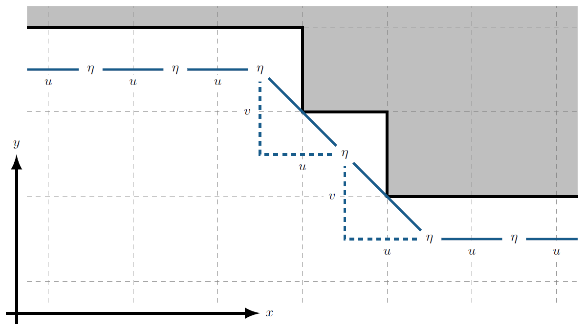
Figure 6 Schematic of the alongshore integration path in GoMSS. The gray area marks the land and the solid black line illustrates the coastline in the model. Solid blue lines illustrate segments of the integration path between grid cells and dashed lines indicate components of diagonal segments.

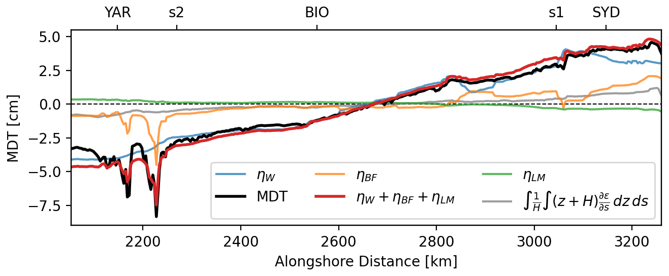
Figure 7 Predicted MDT (black line) and contributions by individual terms in the alongshore, depth-averaged momentum balance at the coast on the Scotian Shelf: wind stress (η_W), bottom friction (η_BF), and lateral mixing (η_LM) as well as their sum. The contribution from the depth-averaged baroclinic pressure gradient is also shown (gray line). Note that the mean of each term has been subtracted to center the curves around zero. Alongshore locations of the tide gauges are shown by their respective abbreviation.

Figure 7 shows the alongshore MDT as well as mean sea level contributions by the individual terms in the momentum balance (Eq. 3) at the coast on the Scotian Shelf. Note that the mean of each term over the shown segment was subtracted to center the curves around zero. The red line shows the sum of the contributions of wind stress, bottom friction, and lateral mixing. It is clearly in close agreement with the MDT along the coast predicted by GoMSS. Including the remaining terms effectively closes the momentum balance defined by Eq. (3).

The alongshore wind stress causes a large-scale tilt of MDT (η_W), with higher values toward Cabot Strait. Along most of the coastline, this wind-driven tilt acts in concert with bottom friction (η_BF) acting on the Nova Scotia Current flowing in the opposite direction of the wind stress at the coast. An exception to this is the region around Sydney where bottom drag is strongest and associated with the Nova Scotia Current flowing close to the coast as it exits the Gulf of Saint Lawrence. Farther downstream, the Nova Scotia Current veers offshore and bottom friction at the coast becomes negligible except in the region around YAR where it balances local MDT minima. These features are due to the Bernoulli effect caused by strong tidal currents around Cape Sable as mentioned above. Variations of the sea level equivalent due to lateral mixing (η_LM) are relatively small along the coast of Nova Scotia. These results show that Δη_c is primarily a response to local Ekman dynamics and spatial variations of bathymetry (Lentz and Fewings, 2012). It is important to note that the bottom friction term depends on the alongshore current and thus implicitly includes the effect of large-scale, non-local forcing.

The close agreement between the coastal MDT and the sum of sea level equivalents due to the wind stress, bottom friction, and lateral mixing predicted by GoMSS is consistent with observational studies for other regions along the eastern seaboard of North America (e.g., Scott and Csanady, 1976; Fewings and Lentz, 2010; Lentz, 2024). They show that the coastal circulation is generally in “frictional equilibrium” (Lentz and Fewings, 2012). The overriding importance of wind stress and bottom friction as a coastal boundary also justifies the choice of Csanady's arrested topographic wave model in Sect. 5.

Previous studies have shown that wind forcing is the dominant driver of sea level variability on the Scotian Shelf on synoptic to interannual timescales (e.g., Thompson, 1986; Schwing, 1989; Li et al., 2014b). Many of these studies also demonstrate the influence of remote forcing and coastally trapped waves propagating along the Scotian Shelf. This is evident in Fig. 7 for alongshore distances > 3100 km, which corresponds to the coastline between SYD and the open boundary across Cabot Strait. Here, the wind-driven sea level tilts in the opposite direction compared to the MDT, which is primarily balanced by bottom friction.

The steric contribution to the alongshore tilt of MDT at the coast is small (0.9 cm between s₁ and s₂, about half of the contribution by bottom friction). This justifies the assumption made in the simplified alongshore momentum equation (Eq. 8). In the cross-shore direction, a large density gradient exists, which is related to the geostrophic outflow from the Gulf of Saint Lawrence with a coastal setup of MDT on the western side of Cabot Strait (El-Sabh, 1977). According to the idealized model of Csanady (1982, Fig. 5), this setup “diffuses” in the downstream direction, with the flow trapped within a widening coastal boundary layer. Note that the associated fanning out of MDT contours is evident in Fig. 3a, which can be compared with the region y<0 in Fig. 5.

6.2 Coastal and regional interpretations of Δη_c

In the following, we apply the dynamical interpretations of Δη_c derived in Sect. 4 to GoMSS. Note that the coastal and regional views are based on time-averaged dynamics and can therefore be applied to shelf circulation on timescales where a quasi-steady state can be assumed.

6.2.1 Coastal view

Based on Eq. (9), Δη_c can be related to the integrated frictional effects along the coast. As shown above, alongshore wind stress is the main contributor to the MDT difference at the coast of Nova Scotia. Since the sea level equivalent due to wind stress can be computed from the GoMSS model output, the special case in Eq. (11) will be used. Given the negligible role of lateral mixing and assuming linear bottom friction ${\mathit{\tau }}_s^{\text{b}}/{\mathit{\rho }}_{\mathrm{0}}=\mathit{\lambda }{\stackrel{\mathrm{‾}}{u}}_s$, the wind-corrected tilt of MDT is proportional to the mean depth-averaged alongshore current:

$$\begin{array}{}\text{(28)}& \langle u_s\rangle ={\displaystyle \frac{\mathrm{1}}{\mathrm{\Delta }L}}\underset{s_{\mathrm{1}}}{\overset{s_{\mathrm{2}}}{\int }}{\stackrel{\mathrm{‾}}{u}}_s\mathrm{d}s.\end{array}$$

It follows from Eq. (11) that the predicted mean depth-averaged alongshore current based on the $\mathrm{\Delta }{\stackrel{\mathrm{̃}}{\mathit{\eta }}}_{\text{c}}$ is

$$\begin{array}{}\text{(29)}& \langle {\stackrel{\mathrm{̃}}{u}}_s\rangle =-{\displaystyle \frac{g{H}_{\mathrm{0}}}{\mathit{\lambda }\mathrm{\Delta }L}}\mathrm{\Delta }{\stackrel{\mathrm{̃}}{\mathit{\eta }}}_{\text{c}},\end{array}$$

where H₀ is the mean depth of the model along the coast.

It is to be expected that λ changes with seasonal stratification of the water column and current variance. Therefore a time-varying friction coefficient is defined by

$$\begin{array}{}\text{(30)}& \mathit{\lambda }={\mathit{\lambda }}_{\mathrm{0}}\mathit{\{}\mathrm{1}+\mathit{\alpha }\cos [(t-t_{\mathrm{0}})\mathit{\omega }\left]\mathit{\right\}},\end{array}$$

where λ₀ is a constant drag coefficient, α is a factor that controls the amplitude of the seasonal variations with frequency $\mathit{\omega }=\mathrm{2}\mathit{\pi }/\mathrm{365}$ d⁻¹, and t₀ corresponds to a time when stratification is at its seasonal maximum and current variance is minimal.

Furthermore, defining $\mathit{\kappa }=g{H}_{\mathrm{0}}/{\mathit{\lambda }}_{\mathrm{0}}\mathrm{\Delta }L$, Eq. (29) becomes

$$\begin{array}{}\text{(31)}& \langle {\stackrel{\mathrm{̃}}{u}}_s\rangle =-{\displaystyle \frac{\mathit{\kappa }}{\mathrm{1}+\mathit{\alpha }\cos \left[\right(t-t_{\mathrm{0}}\left)\mathit{\omega }\right]}}\mathrm{\Delta }{\stackrel{\mathrm{̃}}{\mathit{\eta }}}_{\text{c}},\end{array}$$

which is a model with three parameters that can be applied to estimate the mean alongshore current based on $\mathrm{\Delta }{\stackrel{\mathrm{̃}}{\mathit{\eta }}}_{\text{c}}$.

Figure 8a shows time series of 〈u_s〉 and $\langle {\stackrel{\mathrm{̃}}{u}}_s\rangle$ based on daily mean model output from GoMSS with realistic values of λ₀= $\mathrm{1.3}\times {\mathrm{10}}^{-\mathrm{3}}\mathrm{m}{\mathrm{s}}^{-\mathrm{1}}$, α= 0.5, and t₀= 30 d. These values were chosen to yield maximum agreement between the time series, and λ₀ is comparable to literature values (e.g., Csanady, 1982). The mean water depth along the coast, H₀= 23.4 m, and ΔL= 774 km were directly computed from the GoMSS grid. Based on the definition in Eq. (28), positive values correspond to a southwest flow from s₁ to s₂. Periodograms were analyzed to check if the time series contain an aliased signal from tidal variations. It was found that there is no significant energy at the alias frequencies. A third-order Butterworth low-pass filter with cutoff frequency of 15 d was applied to the time series to remove high-frequency variability and thereby allow a quasi-steady state to be assumed.

Both time series show coherent low-frequency variability for timescales of 15 d or longer with correlation r=0.92. The RMSE between the time series is 1.4 cm s⁻¹. The good agreement between the two time series indicates that the mean strength of the alongshore current can be estimated by the MDT difference at the coast after correction for the local wind effect. However, there is a small offset between the two time series that can be explained by the alongshore gradient of depth-integrated potential energy anomaly. While this term typically vanishes in shallow water, it is nonzero in GoMSS due to the finite water depth along the coast in the model (not shown).

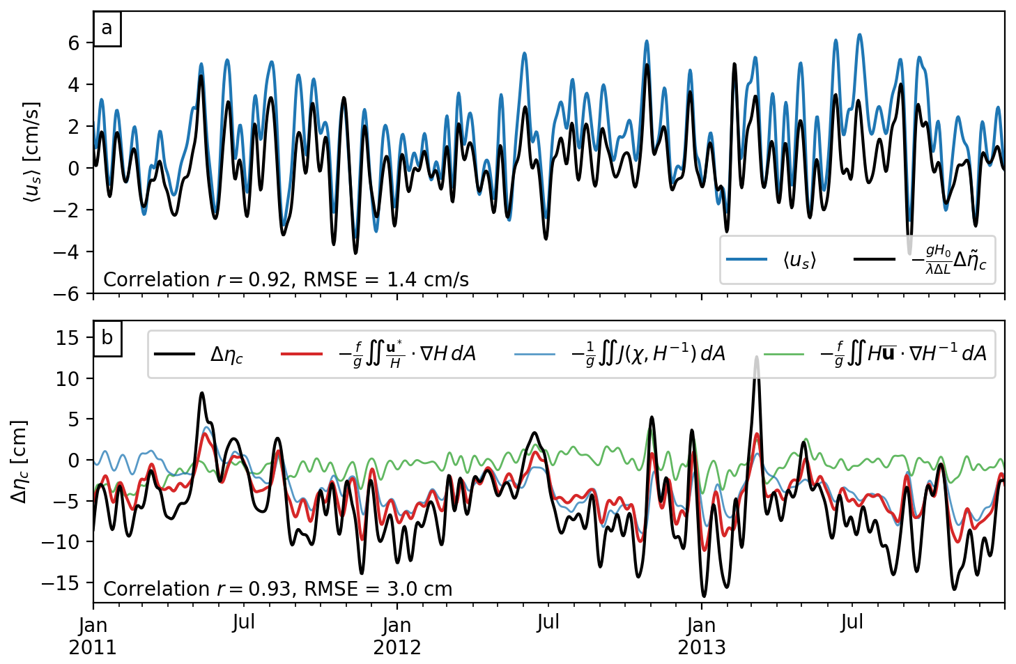
Figure 8 Low-pass-filtered time series of the alongshore tilt of MDT at the coast of Nova Scotia and related quantities. (a) Mean alongshore depth-averaged current predicted by GoMSS (blue) and estimated from wind-corrected tilt of predicted MDT (black). (b) $\mathrm{\Delta }{\mathit{\eta }}_{\text{c}}=\mathit{\eta }\left(s_{\mathrm{2}}\right)-\mathit{\eta }\left(s_{\mathrm{1}}\right)$ predicted by GoMSS (black), diagnostic of area-integrated nearshore circulation (red), area-integrated JEBAR (blue), and flow across isobaths (green). The model output was integrated over the area enclosed by the red polygon in Fig. 1. A third-order Butterworth low-pass filter with a cutoff frequency of 15 d was applied to the time series to remove high-frequency variability and thereby allow a quasi-steady state to be assumed.

6.2.2 Regional view

Equations (15) and (20) relate coastal MDT to area-integrated nearshore ocean circulation as well as wind stress and frictional forces projected along the offshore boundary. Assuming the wind stress and frictional terms are negligible in deep water because of their inverse dependence on H, the tilt of sea level along the coast is then given by

$$\begin{array}{}\text{(32)}& \begin{array}{rl}\mathrm{\Delta }{\mathit{\eta }}_{\text{c}}& =-{\displaystyle \frac{f}{g}}\underset{A}{\iint }{\displaystyle \frac{{\mathit{u}}^{*}}{H}}\cdot \mathrm{\nabla }H\mathrm{d}A\\ & =-{\displaystyle \frac{f}{g}}\underset{A}{\iint }\left[{\displaystyle \frac{\stackrel{\mathrm{‾}}{\mathit{u}}}{H}}\cdot \mathrm{\nabla }H+J\left(\mathit{\chi },H^{-\mathrm{1}}\right)\right]\mathrm{d}A.\end{array}\end{array}$$

Daily mean output from GoMSS has been integrated over the area enclosed by the red polygon in Fig. 1 to calculate each term in Eq. (32) using f= ${\mathrm{10}}^{-\mathrm{4}}{\mathrm{s}}^{-\mathrm{1}}$. High-frequency variability was removed using the same low-pass filter described above, and the resulting time series are shown in Fig. 8b.

There is clearly close agreement between Δη_c and the area-integrated circulation (red line) in terms of both correlation (r=0.93) and RMSE (3.0 cm), with larger discrepancies during extreme events. This can be explained by the assumptions underlying Eq. (32), i.e., the neglect of the wind stress and frictional terms in deep water. Additional analysis (not shown) indicates that the wind-driven sea level difference along the offshore boundaries is not necessarily zero and explains most of the differences. However, the good agreement of the time series demonstrates that the derived relationship between Δη_c and area-integrated nearshore circulation also holds in a realistic model.

Figure 8b also shows the two terms of the second equality in Eq. (32): the area-averaged JEBAR (blue) and the vortex stretching due to depth-averaged flow across isobaths (green). Clearly, the JEBAR contribution is dominant, thereby highlighting the importance of baroclinicity in driving the Nova Scotia Current. The relatively fresh outflow from the Gulf of Saint Lawrence through Cabot Strait causes a strong cross-shore density gradient, leading to a geostrophic flow along the coast.

In general, $\mathrm{\Delta }{\mathit{\eta }}_{\text{c}}=\mathit{\eta }\left(s_{\mathrm{2}}\right)-\mathit{\eta }\left(s_{\mathrm{1}}\right)<\mathrm{0}$, but there are also brief periods when the sign reverses. As shown above, the mean alongshore wind stress creates a sea level tilt along the coast, but it also causes an offshore Ekman transport in the surface boundary layer. This is balanced by a mean onshore flow below determined by the thermal wind balance. Although the wind stress can be uniform over a large area, the associated Ekman transport toward the deeper region offshore leads to a change in relative vorticity. The onshore cross-isobath flow at depth ensures that potential vorticity is conserved.

Similarly, frictional forces at the bottom and JEBAR exert a torque on the water column and generate relative vorticity. While bottom friction leads to an offshore flow across isobaths (see idealized case in Sect. 5.2), JEBAR is dominant along the coast of Nova Scotia. Here it drives an onshore flow that is proportional to Δη_c following Eq. (32), which is captured in the time series shown in Fig. 8b.

7 Summary and conclusion

In this study, we used newly available geodetic estimates of coastal MDT to validate the GoMSS regional ocean model. Additionally, the relationship between coastal MDT and shelf circulation was studied using a combination of theory, idealized models, and a numerical ocean circulation model (GoMSS). It was first shown that GoMSS predicts the main features of the mean circulation that are known to exist on the Scotian Shelf and in the Gulf of Maine, including the effect of outflow from the Gulf of Saint Lawrence and tidal rectification. While the coastal MDT is generally flat in the Gulf of Maine, GoMSS predicts an MDT difference between North Sydney and Yarmouth of Δη_c= 8.3 cm. This is somewhat larger than the geodetically determined value of Δη_c= 5.9±2.0 cm, but the difference is not statistically significant.

These results lead to an affirmative answer to the first question raised in the Introduction: can new observations of geodetically referenced coastal sea level help validate high-resolution regional ocean models like GoMSS? The agreement of the independent estimates of MDT derived from the hydrodynamic and geodetic approaches provides validation of both the ocean and geoid models used in this study. It is important to note that some tide gauges are deployed in geographic settings (e.g., inside harbors or behind sandbanks) that are not resolved by ocean models and where sea level variations are likely dominated by local processes. Therefore, a comparison between observed and predicted MDT is only meaningful in locations that are relatively exposed to the open ocean. At the tide gauges considered in this study, the uncertainties in the geodetic MDT estimates are less than 1.6 cm and are primarily due to estimated errors of the geoid model. With ongoing efforts to improve these models, the uncertainties are expected to become smaller in the future. Nevertheless, the use of Δη_c for model validation is limited to regions with long, geodetically referenced sea level records. In the upper Bay of Fundy, GoMSS predicts an unusually strong set-down in MDT that could not be directly validated because no sufficiently long sea level records exist (see Renkl and Thompson, 2022, for a detailed study of this region).

The other questions addressed in this study focus on the physical interpretation of Δη_c: what can the alongshore tilt of MDT at the coast tell us about shelf circulation? What are the implications for coastal monitoring? Based on theory and idealized models of ocean and shelf circulation, it was shown that Δη_c can be interpreted in two complementary, and dynamically consistent, ways. The coastal view is based on the time-averaged alongshore momentum equation at the coast, and the regional view is based on vorticity dynamics integrated over an adjacent offshore region. The coastally trapped wave model of Csanady (1982) was used to show that Δη_c can be used to estimate spatially averaged net Ekman pumping caused by depth-averaged flow across a linearly sloping bathymetry.

The usefulness of the coastal and regional views was demonstrated in a more realistic setting using output from GoMSS. First, it was shown that the tilt of MDT along the coast of Nova Scotia is balanced primarily by wind stress, bottom friction, and a relatively small contribution from lateral mixing. This “frictional equilibrium” is a general characteristic of coastal circulation (Lentz and Fewings, 2012). This simplified momentum balance means that, if the tilt due to alongshore wind stress is known, Δη_c can provide a direct estimate of the average alongshore current $\langle {\stackrel{\mathrm{̃}}{u}}_s\rangle$ between two points at the coast under the assumption that bottom friction can be approximated by a linear dependence on the depth-averaged flow. The scale factor linking Δη_c and $\langle {\stackrel{\mathrm{̃}}{u}}_s\rangle$ depends only on the mean water depth at the coast and the linear bottom drag coefficient. For practical applications, when the water depth cannot be inferred from a numerical model with a sidewall, it could presumably be determined from bathymetric soundings as the mean water depth along the coast outside the surf zone.

The regional view is more subtle than the coastal view. In idealized models, Δη_c can be used to approximate vortex stretching associated with cross-isobath flow averaged over an offshore area. For the regional view to be physically meaningful, this area needs to be limited to a flow regime in the nearshore region such that the dominant momentum balance simplifies along the offshore integration path. In the illustration of the realistic case using GoMSS, we chose the outer edge of the integration path in a quiescent region outside the Nova Scotia Current where the water is deep enough that wind stress and frictional terms can be neglected. Where the current crosses the integration path, it is in geostrophic balance.

On the Scotian Shelf, the regional interpretation of Δη_c is dominated by JEBAR, while the effect of the depth-averaged flow across isobaths is small. JEBAR plays a critical role and causes an overall onshore transport that balances the offshore wind-driven Ekman transport at the surface, resulting in upwelling at the coast. This overriding importance of baroclinic processes is presumably a distinct feature of the Nova Scotia Current due to the strong freshwater input from the Gulf of Saint Lawrence. In other regions along the eastern seaboard of North America, e.g., in the Mid-Atlantic Bight, where sea level variations depend primarily on alongshore wind stress (Lentz, 2024), the regional view would likely be dominated by the effect of depth-averaged flow across isobath.

The relationship between Δη_c and the coastal and regional circulation applies not only to the long-term mean, but also on timescales for which a quasi-steady state can be assumed. Diagnostic time series shown in Fig. 8 were calculated directly from GoMSS output using simple linear relationships resulting from the coastal and regional views. The parameters in these linear relationships are based on physics. The tilt-based estimates are in good agreement with the filtered time series calculated directly from model output.

This close relationship between coastal MDT and integrated nearshore circulation highlights the utility and value of tilt estimates based on geodically referenced sea level observations for model validation. Furthermore, it also has obvious implications for ocean monitoring: for example, it may be possible to use long coastal sea level records to estimate time series of integrated nearshore circulation and potentially link them to upwelling. Such information may be of interest to biological oceanographers interested in understanding changes in nutrient cycling on the shelf over recent decades. This speculation applies not only to the Scotian Shelf. For example, in the future, it would be interesting to test the idea on the west coast of North America given the large number of long, geodetically referenced sea level records (e.g., Lin et al., 2015) and the large amount of hydrographic data, e.g., the California Cooperative Oceanic Fisheries (CalCOFi) Database. Finally, our findings have implications for future deployments of tide gauges if they are to be used to monitor the shelf-scale ocean circulation. Coastal MDT can be affected by local processes, e.g., strong tidal flow around headlands, and therefore the location of the tide gauges should be exposed to the open ocean and at a distance from areas where local processes dominate.