Seasonality of meridional overturning in the subpolar North Atlantic: density flux as a metric for understanding the Atlantic meridional overturning circulation

The Atlantic meridional overturning circulation (AMOC) has a notable seasonal component. This influences the jet stream and the location, frequency, and intensity of extreme weather events. Understanding this seasonality is important for mitigating the impacts of AMOC changes on European weather and climate. Here, we place meridional overturning and fluxes in a coherent framework. This framework highlights the integral relationship between meridional overturning circulation and property transports, both being functions purely of the overturning streamfunction Ψ. Using this framework, we examine the seasonality observed in overturning and density, temperature, and freshwater fluxes at the Overturning in the Subpolar North Atlantic Program (OSNAP) line in the subpolar North Atlantic. We find the seasonal cycle of the MOC metric (the standard measure of overturning, defined as the maximum of the overturning streamfunction) to be dominated by Ekman transports and the large-scale seasonal cycle of surface density; heat flux to be dominated by barotropic velocity variability; the seasonal cycle of freshwater flux to be dominated by a combination of barotropic velocities and the salinity in the western boundary current; and density flux to reflect a broad range of characteristics and processes. We show that the MOC metric is a poor predictor, on seasonal timescales, of either density fluxes or the more societally relevant ocean heat and freshwater transports. This is due to each of these metrics responding to different physical processes. The MOC metric, on seasonal timescales at least, has very high sensitivity to near-surface physical characteristics in a limited geographical area. These characteristics are not necessarily reflective of the fundamental processes driving overturning. Therefore, we suggest caution in the use of the standard MOC metric when studying overturning and the routine use of the density flux as a valuable additional overturning metric.

1 Introduction

The Atlantic meridional overturning circulation (AMOC) has a notable seasonal component. This influences the jet stream and the location, frequency, and intensity of extreme weather events. Understanding this seasonality is important for mitigating the impacts of AMOC changes on European weather and climate. Driven by innovation in ocean observation, theory, and modelling, our understanding of subpolar North Atlantic meridional overturning has advanced rapidly in recent years. Basin-wide observational arrays, particularly OSNAP (Overturning in the Subpolar North Atlantic Program, Lozier et al., 2019), now allow robust estimation of the seasonal cycle in the strength of subpolar overturning and associated heat and freshwater transports (Gary et al., 2018; Fu et al., 2023a; Fraser et al., 2024; Mercier et al., 2024). Theoretical models of overturning (see Johnson et al., 2019, for a review of the state of the art) help us understand the interplay between surface buoyancy and wind forcing and provide new paradigms for deep water formation. Coupled models (e.g. Swingedouw et al., 2007; Böning et al., 2016; Weijer et al., 2020; Baker et al., 2023, 2025; Madan et al., 2023) help to better understand AMOC feedback mechanisms between ocean and atmosphere, generally predicting AMOC weakening during the 21st century, driven by freshwater input and reduced surface cooling – though results still vary widely. Meanwhile, global-scale high-resolution ocean models (e.g. Hirschi et al., 2020; Biastoch et al., 2021) and state estimates (Forget et al., 2015) allow us to make detailed examination of fine-scale dynamics and mechanisms driving AMOC variability at shorter timescales.

While the driving processes of the AMOC – winds, surface fluxes, and freshwater input – have marked seasonal cycles at subpolar latitudes, it remains unclear how, or if, these seasonal cycles are expressed in the observations of AMOC and related transports on basin-wide sections such as OSNAP. Observational and modelling studies of subpolar North Atlantic meridional overturning consistently return estimates of the seasonal cycle of overturning, as measured by the maximum of the overturning streamfunction (MOC_σ), with an amplitude of about 4 Sv and with a late spring maximum and an autumn or a winter minimum (Lozier et al., 2019; Fu et al., 2023a; Wang et al., 2021; Tooth et al., 2023; Mercier et al., 2024). These studies find overturning seasonality, as for the mean subpolar overturning (Lozier et al., 2019; Petit et al., 2020), to be dominated by water transformation north of a line linking Greenland and Scotland rather than in the Labrador Sea.

Analyses of OSNAP observations (Fu et al., 2023a) show the subpolar AMOC seasonal cycle to be dominated by seasonality in the Irminger Basin, particularly the East Greenland Current, modified by Ekman transport driven by seasonality in the zonal winds. The East Greenland Current seasonality is ascribed to a lagged signal of water mass transformation in the Irminger Basin. Examination of an ocean reanalysis (Wang et al., 2021) and detailed observations (Le Bras et al., 2020) suggest that the seasonal cycle of overturning closely follows density variability in the western boundary current. However, other observations show (Mercier et al., 2024; Le Bras et al., 2018) the seasonal transport variability in the western boundary current also to be an important contributor to the AMOC seasonal cycle. The combined effect of density and transport seasonality is explored in results from a high-resolution ocean hindcast model (Tooth et al., 2023), with innovative use of Lagrangian tracking to attribute transport variability to variability of particle transit times around the northern subpolar Gyre. Seasonality in zonal winds is a common theme dominating MOC seasonality at lower latitudes (Yang, 2015; Zhao and Johns, 2014), with geostrophic transport at the boundaries and in the interior, perhaps in turn driven by wind-stress curl or a lagged response to deep-water formation, controlling the seasonal cycle at higher latitudes (Chidichimo et al., 2010; Zhao and Johns, 2014; Gary et al., 2018; Tooth et al., 2023; Mercier et al., 2024).

The maximum of the overturning streamfunction, integrated across the width of the basin and calculated variously in density (MOC_σ) or depth (MOC_z) space, has become synonymous with the strength of the meridional overturning circulation on a given transatlantic section. Indeed, we will use it in this sense in the current work. In a wider, ocean conveyor belt sense, in the North Atlantic and Arctic basins, the meridional overturning circulation is fundamentally a water transformation process – lighter surface waters flowing northward, being transformed into denser waters, sinking, mixing, and then flowing southward. Observational arrays such as OSNAP (Lozier et al., 2019) and RAPID (Cunningham et al., 2007; Kanzow et al., 2007) attempt to quantify these transformation processes by monitoring the north–south exchanges along basin-wide sections. On shorter, seasonal, and interannual timescales, it is clear that the “overturning” signal observed at these arrays does not purely represent this wider, large-scale overturning. Adiabatic, “sloshing” motions (Han, 2023a, b; Fraser et al., 2025) driven by Ekman transport and wind-stress curl (Fraser et al., 2024) dominate observed MOC_σ on shorter timescales. Seasonal cycles of surface mixed layer warming and cooling, deepening, and shallowing will also be expressed in the seasonal cycle of the overturning streamfunction, even where these changes are not ultimately subducted into the ocean interior and the overturning circulation (Tooth et al., 2023).

Here, we attempt to disentangle the various processes expressed in the MOC_σ and overturning streamfunction at the OSNAP line. To do this, we adopt and extend the formalism proposed by Mercier et al. (2024). This formalism allows us to separate out components of the overturning streamfunction seasonal variability associated with, for example, surface Ekman transports, water transformation, or velocity variability. We use these methods to examine the seasonal cycle in the full density-space overturning streamfunction, rather than focussing exclusively on MOC_σ (the maximum of the streamfunction). We also introduce an additional metric based on the overturning streamfunction, i.e. the “density flux”, calculated as the area under the overturning streamfunction curve (e.g. Fraser and Cunningham, 2021). This density flux is a somewhat neglected part of the water mass transformation theory (Tziperman, 1986; Speer and Tziperman, 1992; Nurser et al., 1999) that fundamentally underpins the concept of overturning and has close parallels with both heat and freshwater transports. The density flux arises from mass conservation, rather than from volume conservation as for MOC_σ, with density flux northward across a meridional section largely balanced by total surface density fluxes over the region north of the section in the longer term. This contrasts with MOC_σ, which balances surface fluxes over the narrow outcrop region of a single isopycnal and diapycnal mixing across that isopycnal. Thus, density flux complements MOC_σ to give a more complete understanding of overturning. Using this framework, beginning with analysis of the output of a high-resolution model hindcast, we aim to produce a more comprehensive and integrated description of the seasonal cycle of overturning observed on the OSNAP line, encompassing MOC_σ, density flux, and heat and freshwater transports. We consider how each of these important overturning metrics responds differently to the underlying mechanisms driving the overturning. The model-derived hypotheses obtained are then tested against the seasonal cycle in the OSNAP observational time series, and possible implications for AMOC and climate studies examining variability on longer timescales are discussed.

2 Methods

2.1 Data

We make use of the eddy-rich, nested ocean–sea-ice model configuration VIKING20X; full details are given in Biastoch et al. (2021) and will not be repeated here, and the data are available from Getzlaff and Schwarzkopf (2024). Briefly, in the vertical direction, VIKING20X uses 46 geopotential z levels with layer thicknesses gradually increasing from 6 m at the surface to 250 m in the deepest layers. The bottom topography is represented by partially filled cells. In the horizontal direction, VIKING20X has a tripolar grid with 0.25° global resolution, which is refined in the Atlantic Ocean to 0.05°, yielding an effective grid spacing of 3–4 km in the subpolar North Atlantic. The run used here, VIKING20X-JRA-short, is an experiment forced from 1980 to 2019 by the JRA55-do forcing (version 1.4) (Tsujino et al., 2018). Hindcasts of the past 50–60 years in this eddy-rich configuration realistically simulate the large-scale horizontal circulation, including the AMOC, the distribution of the mesoscale, overflow, and convective processes, and the representation of regional current systems in the North and South Atlantic (Biastoch et al., 2021; Rühs et al., 2021). For consistency with the observations, we based our calculations on monthly mean model output. Model results presented in the main text are based on the final 20 years of this run, i.e. 2000–2019 (the Supplement contains results based on the 2014–2019 period to more closely match the observational period).

For the observational analysis, we use the OSNAP 6-year gridded dataset and time series (Fu et al., 2023a, b) and the ERA5 surface wind stress (Hersbach et al., 2020, 2023). For parts of the analysis, we divide the OSNAP line at Greenland into OSNAP west (OSNAP_W) and OSNAP east (OSNAP_E). ERA5 wind stresses are interpolated onto the OSNAP gridded observation points and used to calculate Ekman transports across the OSNAP section. The location of the OSNAP section is shown in Fig. 1.

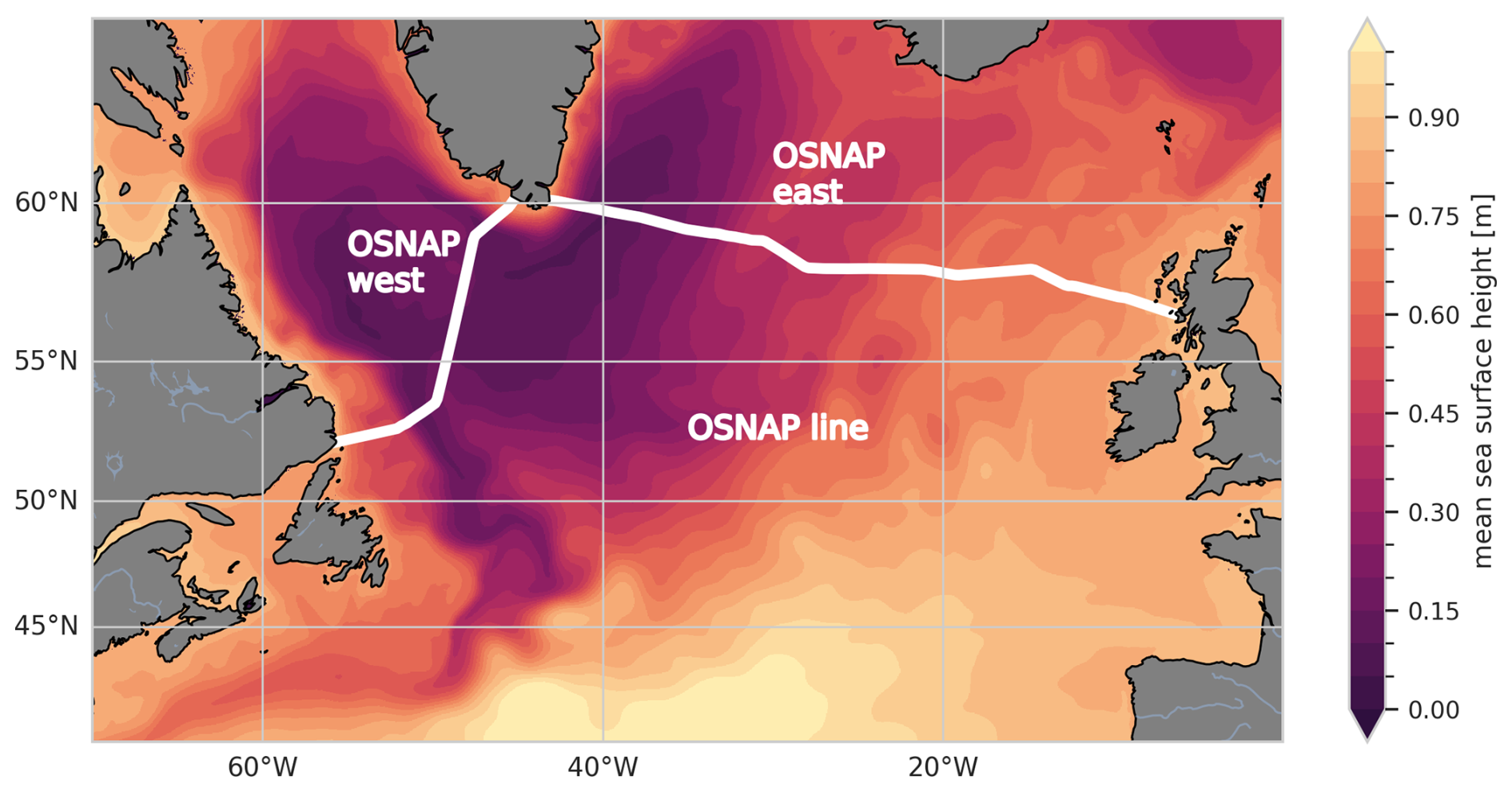
Figure 1 The location of the OSNAP observing line. We use OSNAP west to refer to the section across the Labrador Sea west of Greenland and OSNAP east to refer to the section from Greenland to Scotland. The colour scale represents the 20-year mean sea surface height from the VIKING20X model.

2.2 Theoretical framework

The zonally integrated overturning streamfunction in density space, Ψ_σ(σ,t), can be written as:

$$\begin{array}{}\text{(1)}& {\displaystyle }{\displaystyle }{\mathrm{\Psi }}_{\mathit{\sigma }}\left(\mathit{\sigma },t\right)=\underset{R\left(\mathit{\sigma },t\right)}{\iint }v\left(x,z,t\right)\mathrm{d}z\mathrm{d}x,\end{array}$$

where R(σ,t) is the part of the (x,z) vertical plane defined by ${\mathit{\sigma }}_{\text{min}}<{\mathit{\sigma }}^{\prime }(x,z,t)<\mathit{\sigma }$, that is, we integrate over the area with potential density less than σ. Here, $x\in [w,e]$ is the along-section coordinate, $z\in [-H,\mathit{\eta }]$ is the vertical coordinate (positive upward), and $v(x,z,t)$ is the velocity normal to the section at time t. The fixed horizontal section end points are given by w,e; H(x) is the water depth; and η(x,t) the sea surface height.

The overturning streamfunction Ψ has units of m³ s⁻¹ or, more commonly, Sv (Sverdrup, where 1 Sv = 1×10⁶ m³ s⁻¹). Note that we choose to integrate from low to high density. The direction of integration makes no difference when the total volume transport through the section is zero. On the OSNAP line, there is generally a small net southward flow, integrating from high to low density, that then leads to small offsets in overturning and transports. Importantly, for the work presented here, the direction of integration has very little impact on the anomalies (no impact for the observations where net transports are fixed).

We then define, in the usual way, the meridional overturning, MOC_σ(t), as the maximum of Ψ_σ for all σ and σ_MOC(t) as the density at which this maximum occurs:

$$\begin{array}{}\text{(2)}& {\displaystyle }& {\displaystyle }{\text{MOC}}_{\mathit{\sigma }}\left(t\right)=\underset{\mathit{\sigma }}{max}\left[{\mathrm{\Psi }}_{\mathit{\sigma }}(\mathit{\sigma },t)\right],\text{(3)}& {\displaystyle }& {\displaystyle }{\mathit{\sigma }}_{\text{MOC}}\left(t\right)={\text{arg\hspace{0.17em}max}}_{\mathit{\sigma }}\left[{\mathrm{\Psi }}_{\mathit{\sigma }}(\mathit{\sigma },t)\right].\end{array}$$

Here, we introduce a further metric, i.e. the northward meridional density flux (𝒟):

$$\begin{array}{}\text{(4)}& {\displaystyle }{\displaystyle }\mathcal{D}\left(t\right)=-\underset{{\mathit{\sigma }}_{\text{min}}}{\overset{{\mathit{\sigma }}_{\text{max}}}{\int }}{\mathrm{\Psi }}_{\mathit{\sigma }}\mathrm{d}\mathit{\sigma }.\end{array}$$

This density flux forms a part of water mass transformation theory (Tziperman, 1986; Speer and Tziperman, 1992; Nurser et al., 1999); here, we consider only the case where we integrate over the full density range $({\mathit{\sigma }}_{\text{min}}<\mathit{\sigma }<{\mathit{\sigma }}_{\text{max}})$. We follow convention in referring to this as “density flux”, while the units of kg s⁻¹ perhaps suggest “mass flux”. It is not a true mass flux, as steric height changes are ignored in both model (via the Boussinesq approximation) and observational (surface defined as z=0) calculations. The term “density flux” captures the process intuitively – with lighter water flowing northward and denser water returning southward being characterised as a southward (or negative northward) density flux. This metric is easily visualised as the area under the density-space streamfunction curves in Figs. 2 and 3.

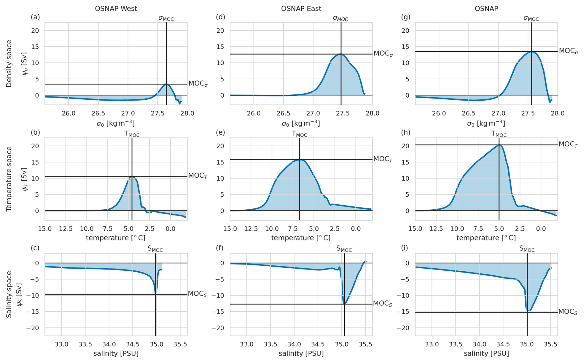
Figure 2 Mean overturning streamfunctions from 20 years of the Viking20x model. The left-hand column (a–c) shows OSNAP_W, the centre column (d–f) OSNAP_E, and the right-hand column (g–i) the full OSNAP transect. In each case, the top row (a, d, g) is the overturning streamfunction in density space, the middle row (b, e, h) in temperature space, and the bottom row (c, f, i) in salinity space. The maximum overturning (negative in salinity space) is highlighted in each case, labelled MOC, along with the property value at which it occurs (σ_MOC for density, T_MOC for temperature, and S_MOC for salinity). The shaded integrated areas under the curve are proportional to the southward density flux (a, d, g), the northward heat flux (b, e, h), and the northward freshwater flux (c, f, i; negative shows that net freshwater flux is southward). The plots are scaled such that unit area in each case very approximately corresponds to the same density flux – MOC_σ and the southward density flux are a combination of the northward heat flux opposed by the southward freshwater flux.

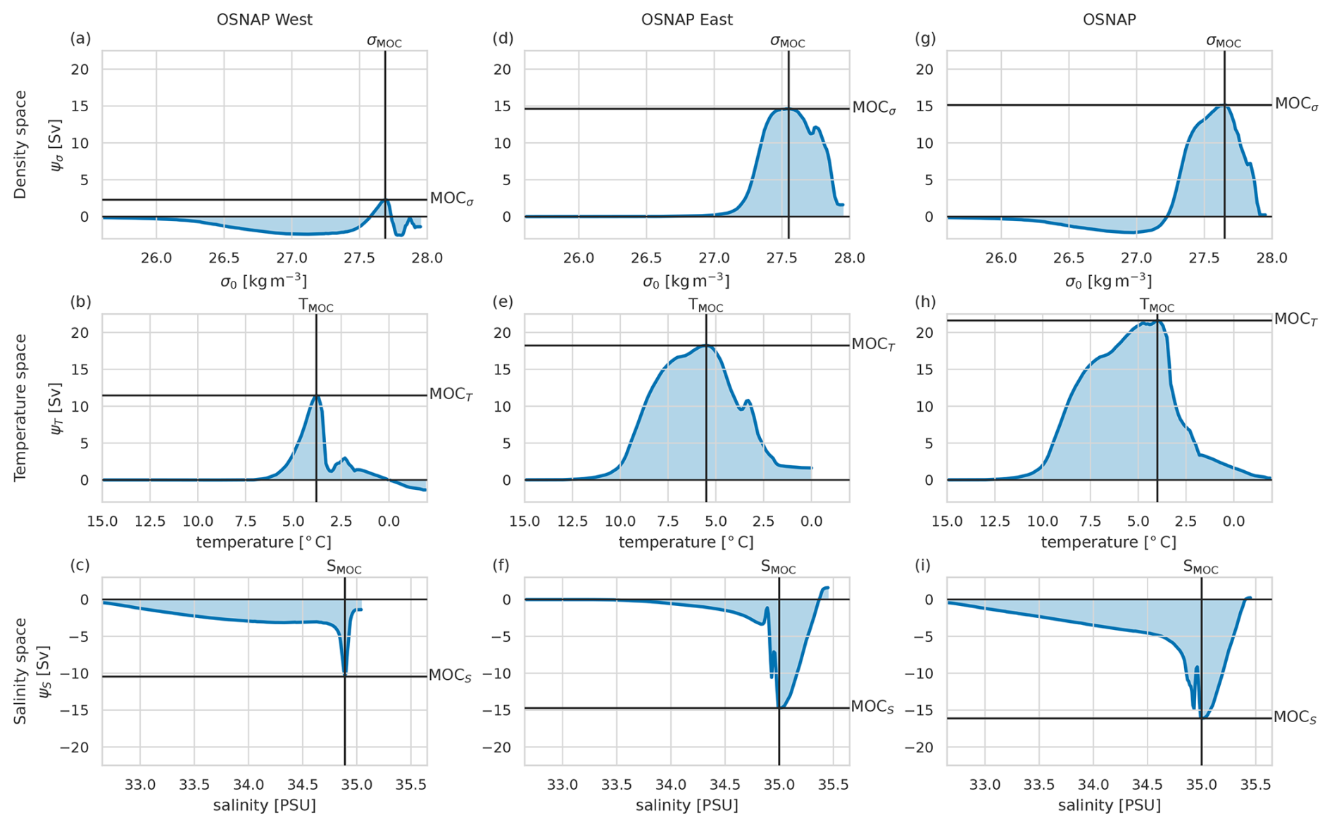
Figure 3 Same as for Fig. 2 but for the overturning from the 6-year OSNAP observational time series.

Rearranging Eq. (4), we can write this density flux and perhaps gain some physical insight. Changing the coordinate from σ to z and integrating by parts, Eq. (4) becomes:

$$\begin{array}{}\text{(5)}& {\displaystyle }{\displaystyle }\mathcal{D}=\underset{w}{\overset{e}{\int }}\underset{-H}{\overset{\mathit{\eta }}{\int }}v\mathit{\sigma }\mathrm{d}z\mathrm{d}x-{\mathit{\sigma }}_{\text{max}}\underset{w}{\overset{e}{\int }}\underset{-H}{\overset{\mathit{\eta }}{\int }}v\mathrm{d}\mathit{\sigma }\mathrm{d}x.\end{array}$$

The second term on the right-hand side of Eq. (5) is a multiple of the net volume transport through the section. If this net volume transport is zero – a useful approximation for the transoceanic sections considered here and the one imposed in the construction of the OSNAP observational overturning transports – the density flux (𝒟) reduces to simply the integral of vσ over the section. If the net volume flux is non-zero, however, the right-hand side of Eq. (5) can become the difference between two large terms. We can further rewrite Eq. (5) as the integrated northward transport of density relative to reference density σ_max:

$$\begin{array}{}\text{(6)}& {\displaystyle }{\displaystyle }\mathcal{D}=\underset{w}{\overset{e}{\int }}\underset{-H}{\overset{\mathit{\eta }}{\int }}v(\mathit{\sigma }-{\mathit{\sigma }}_{\text{max}})\mathrm{d}z\mathrm{d}x.\end{array}$$

For the streamfunction anomalies discussed here, all terms involving the reference density σ_max drop out for the observations, as the net volume transport across each section is constant by construction. However, in the model, the net volume transport varies in time (though it is always small compared to the overturning transport). At the suggestion of an anonymous reviewer, we repeated calculations after adding a uniform “compensation” velocity to the model at each time step to fix the net transports at their mean value. This made very little quantitative, and no qualitative, difference to the results.

A quick note on terminology: throughout, we use the terms “overturning streamfunction” to refer to Ψ(σ,t) and “meridional overturning” or “MOC” to refer to the maximum of Ψ in density space.

Note that the density-space equations have analogues in both temperature and salinity space; for the sake of brevity and clarity, we will discuss temperature and salinity space results only briefly, and purely in the context of heat and freshwater transports, but the relevant equations are given here. In temperature, or θ, space, we have the overturning streamfunction (Ψ_θ), meridional overturning (MOC_θ at temperature θ_MOC), and meridional heat transport (ℋ). We choose to integrate downward in temperature space, from high to low, which reverses the sign in the heat transport equation below:

$$\begin{array}{}\text{(7)}& {\displaystyle }{\displaystyle }{\mathrm{\Psi }}_{\mathit{\theta }}\left(\mathit{\theta },t\right)=\underset{R\left(\mathit{\theta },t\right)}{\iint }v\left(x,z,t\right)\mathrm{d}z\mathrm{d}x,\end{array}$$

where R(θ,t) is the area defined by $\mathit{\theta }<{\mathit{\theta }}^{\prime }(x,z,t)<{\mathit{\theta }}_{\text{max}}$:

$$\begin{array}{}\text{(8)}& {\displaystyle }& {\displaystyle }{\text{MOC}}_{\mathit{\theta }}\left(t\right)=\underset{\mathit{\theta }}{max}\left[{\mathrm{\Psi }}_{\mathit{\theta }}(\mathit{\theta },t)\right],\text{(9)}& {\displaystyle }& {\displaystyle }{\mathit{\theta }}_{\text{MOC}}\left(t\right)={\text{arg\hspace{0.17em}max}}_{\mathit{\theta }}\left[{\mathrm{\Psi }}_{\mathit{\theta }}(\mathit{\theta },t)\right],\text{(10)}& {\displaystyle }& {\displaystyle }\mathcal{H}=\mathit{\rho }{C}_p\underset{{\mathit{\theta }}_{\text{min}}}{\overset{{\mathit{\theta }}_{\text{max}}}{\int }}{\mathrm{\Psi }}_{\mathit{\theta }}\mathrm{d}\mathit{\theta },\end{array}$$

where ρ is the potential density and C_p the specific heat capacity of sea water. Finally, in salinity, or S, space, we have the overturning streamfunction (Ψ_S), meridional overturning (MOC_S at salinity S_MOC), and northward meridional freshwater transport (ℱ). In salinity space, the sign of the overturning streamfunction is usually reversed, with net freshwater input in the north opposing the overturning. Thus, we define MOC_S(t) as the minimum of Ψ_S rather than the maximum. We also convert northward salinity transports to freshwater transports using a section mean reference salinity, $\stackrel{\mathrm{‾}}{S}$. Hence,

$$\begin{array}{}\text{(11)}& {\displaystyle }{\displaystyle }{\mathrm{\Psi }}_S\left(S,t\right)=\underset{R\left(S,t\right)}{\iint }v\left(x,z,t\right)\mathrm{d}z\mathrm{d}x,\end{array}$$

where R(S,t) is the area defined by $S_{\text{min}}<S^{\prime }(x,z,t)<S$:

$$\begin{array}{}\text{(12)}& {\displaystyle }& {\displaystyle }{\text{MOC}}_S\left(t\right)=\underset{S}{min}\left[{\mathrm{\Psi }}_S(S,t)\right],\text{(13)}& {\displaystyle }& {\displaystyle }{S}_{\text{MOC}}\left(t\right)={\text{arg\hspace{0.17em}min}}_S\left[{\mathrm{\Psi }}_S(S,t)\right],\text{(14)}& {\displaystyle }& {\displaystyle }\mathcal{F}={\displaystyle \frac{\mathrm{1}}{\stackrel{\mathrm{‾}}{S}}}\underset{S_{\text{min}}}{\overset{S_{\text{max}}}{\int }}{\mathrm{\Psi }}_S\mathrm{d}S.\end{array}$$

These relationships are displayed graphically for the mean overturning streamfunctions in Figs. 2 and 3. Using this framework, it becomes clear that the overturning and property transport metrics are intimately linked. Considering density space, MOC is the extreme of the streamfunction Ψ, σ_MOC the position of that extreme, and density flux the area under the streamfunction curve. We can imagine scenarios in which variability of these could be either strongly correlated or entirely decoupled: increasing the northward volume transport in the upper limb (and, by extension, the southward volume transport in the lower limb) would increase both MOC and density flux, but reducing the density of northward-flowing waters, for example, would increase the area under the density flux, though MOC may be unaffected (the effect on MOC will depend on the density of the waters involved and how that relates to σ_MOC).

2.3 Streamfunction decomposition

We decompose the streamfunction variability into parts associated with velocity variability, density structure variability, and covariation of density and velocity fields following Mercier et al. (2024). This decomposition helps us to examine the individual and combined influence on the seasonal cycle particular forcing, for example, wind stress and surface density fluxes.

Rewriting Eq. (1), we have:

$$\begin{array}{}\text{(15)}& {\displaystyle }{\displaystyle }{\mathrm{\Psi }}_{\mathit{\sigma }}\left(\mathit{\sigma },t\right)=\underset{w}{\overset{e}{\int }}\underset{z_{\mathit{\sigma }}\left(\mathit{\sigma }\right)}{\overset{\mathit{\eta }}{\int }}v(x,z,t)\mathrm{d}z\mathrm{d}x,\end{array}$$

where $z_{\mathit{\sigma }}\left(\mathit{\sigma }\right)=z_{\mathit{\sigma }}(\mathit{\sigma },x,t)$ is the depth of the σ isopycnal at position x and time t.

We can decompose the velocity field into time-mean, $\stackrel{\mathrm{‾}}{v}$, and variable, v^′, parts and the isopycnal depths into a time-mean part, ${\stackrel{\mathrm{‾}}{z}}_{\mathit{\sigma }}$, and a deviation from the time-mean, $z_{\mathit{\sigma }}^{\prime }$. These time-means are calculated over the full length of the relevant dataset, so 6 years for the observations and 20 years for the model (6 years for the results from the shorter model time series included as SI).

$$\begin{array}{}\text{(16)}& {\displaystyle }& {\displaystyle }v=\stackrel{\mathrm{‾}}{v}+v^{\prime }\text{(17)}& {\displaystyle }& {\displaystyle }{z}_{\mathit{\sigma }}={\stackrel{\mathrm{‾}}{z}}_{\mathit{\sigma }}+z_{\mathit{\sigma }}^{\prime }\end{array}$$

We can then rewrite Eq. (15) as:

$$\begin{array}{ll}{\displaystyle }{\mathrm{\Psi }}_{\mathit{\sigma }}\left(\mathit{\sigma },t\right)=& {\displaystyle }\underset{w}{\overset{e}{\int }}\underset{{\stackrel{\mathrm{‾}}{z}}_{\mathit{\sigma }}\left(\mathit{\sigma }\right)+z_{\mathit{\sigma }}^{\prime }(\mathit{\sigma },t)}{\overset{\mathit{\eta }}{\int }}\stackrel{\mathrm{‾}}{v}(x,z)\mathrm{d}z\mathrm{d}x\\ \text{(18)}& {\displaystyle }& {\displaystyle }+\underset{w}{\overset{e}{\int }}\underset{{\stackrel{\mathrm{‾}}{z}}_{\mathit{\sigma }}\left(\mathit{\sigma }\right)+z_{\mathit{\sigma }}^{\prime }(\mathit{\sigma },t)}{\overset{\mathit{\eta }}{\int }}{v}^{\prime }(x,z,t)\mathrm{d}z\mathrm{d}x{\displaystyle }=& {\displaystyle }\underset{\text{mean}}{\underbrace{\underset{w}{\overset{e}{\int }}\underset{{\stackrel{\mathrm{‾}}{z}}_{\mathit{\sigma }}\left(\mathit{\sigma }\right)}{\overset{\mathit{\eta }}{\int }}\stackrel{\mathrm{‾}}{v}\mathrm{d}z\mathrm{d}x}}+\underset{\text{density variation}}{\underbrace{\underset{w}{\overset{e}{\int }}\underset{{\stackrel{\mathrm{‾}}{z}}_{\mathit{\sigma }}\left(\mathit{\sigma }\right)+z_{\mathit{\sigma }}^{\prime }(\mathit{\sigma },t)}{\overset{{\stackrel{\mathrm{‾}}{z}}_{\mathit{\sigma }}\left(\mathit{\sigma }\right)}{\int }}\stackrel{\mathrm{‾}}{v}\mathrm{d}z\mathrm{d}x}}\\ \text{(19)}& {\displaystyle }& {\displaystyle }+\underset{\text{velocity variation}}{\underbrace{\underset{w}{\overset{e}{\int }}\underset{{\stackrel{\mathrm{‾}}{z}}_{\mathit{\sigma }}\left(\mathit{\sigma }\right)}{\overset{\mathit{\eta }}{\int }}{v}^{\prime }\mathrm{d}z\mathrm{d}x}}+\underset{\text{density-velocity covariation}}{\underbrace{\underset{w}{\overset{e}{\int }}\underset{{\stackrel{\mathrm{‾}}{z}}_{\mathit{\sigma }}\left(\mathit{\sigma }\right)+z_{\mathit{\sigma }}^{\prime }(\mathit{\sigma },t)}{\overset{{\stackrel{\mathrm{‾}}{z}}_{\mathit{\sigma }}\left(\mathit{\sigma }\right)}{\int }}{v}^{\prime }\mathrm{d}z\mathrm{d}x}},\end{array}$$

where the first two terms on the right-hand side integrate the time-mean velocity field and the last two integrate the velocity anomalies. The first and third terms on the right-hand side are integrals between the depth of the time-mean σ isopycnal and the surface, and the second and fourth terms integrate between the instantaneous and time-mean isopycnal depths. We write this more concisely as:

$$\begin{array}{ll}{\displaystyle }{\mathrm{\Psi }}_{\mathit{\sigma }}\left(\mathit{\sigma },t\right)=& {\displaystyle }{\mathrm{\Psi }}_{\stackrel{\mathrm{‾}}{\mathit{\sigma }}\stackrel{\mathrm{‾}}{v}}\left(\mathit{\sigma }\right)+{\mathrm{\Psi }}_{{\mathit{\sigma }}^{\prime }\stackrel{\mathrm{‾}}{v}}\left(\mathit{\sigma },t\right)+{\mathrm{\Psi }}_{\stackrel{\mathrm{‾}}{\mathit{\sigma }}{v}^{\prime }}\left(\mathit{\sigma },t\right)\\ \text{(20)}& {\displaystyle }& {\displaystyle }+{\mathrm{\Psi }}_{{\mathit{\sigma }}^{\prime }{v}^{\prime }}\left(\mathit{\sigma },t\right).\end{array}$$

Removing the long-term mean ($\stackrel{\mathrm{‾}}{{\mathrm{\Psi }}_{\mathit{\sigma }}}$) from all terms and taking monthly means to examine the seasonal cycle leave:

$$\begin{array}{ll}{\displaystyle }{\mathrm{\Psi }}_{\mathit{\sigma }}^{\prime }\left(\mathit{\sigma },m\right)=& {\displaystyle }{\mathrm{\Psi }}_{{\mathit{\sigma }}^{\prime }\stackrel{\mathrm{‾}}{v}}^{\prime }\left(\mathit{\sigma },m\right)+{\mathrm{\Psi }}_{\stackrel{\mathrm{‾}}{\mathit{\sigma }}{v}^{\prime }}^{\prime }\left(\mathit{\sigma },m\right)\\ \text{(21)}& {\displaystyle }& {\displaystyle }+{\mathrm{\Psi }}_{{\mathit{\sigma }}^{\prime }{v}^{\prime }}^{\prime }\left(\mathit{\sigma },m\right),\end{array}$$

where m now indicates that these are mean monthly anomalies from the long-term mean.

We further decompose the velocity anomaly into a surface-Ekman-driven component, $v_{\text{Ek}}^{\prime }(x,z,t)$ (calculated from the wind stress, with uniform compensating flow below the surface layer), and a remainder, $v^{\prime \prime }(x,t)$.

$$\begin{array}{}\text{(22)}& {\displaystyle }{\displaystyle }{\mathrm{\Psi }}_{\stackrel{\mathrm{‾}}{\mathit{\sigma }}{v}^{\prime }}^{\prime }\left(\mathit{\sigma },m\right)={\mathrm{\Psi }}_{\stackrel{\mathrm{‾}}{\mathit{\sigma }}{v}_{\text{Ek}}^{\prime }}^{\prime }\left(\mathit{\sigma },m\right)+{\mathrm{\Psi }}_{\stackrel{\mathrm{‾}}{\mathit{\sigma }}{v}^{\prime \prime }}^{\prime }\left(\mathit{\sigma },m\right)\end{array}$$

The density anomaly is decomposed in two ways, applied independently. Firstly, it is decomposed into a part due to temperature anomalies (with salinity held at the long-term mean) ${\mathit{\sigma }}_T^{\prime }$, a part due to salinity anomalies (with temperature held at the long-term mean) ${\mathit{\sigma }}_S^{\prime }$, and ${\mathit{\sigma }}_{TS}^{\prime }$ due to the nonlinearities in the equation of state:

$$\begin{array}{ll}{\displaystyle }{\mathrm{\Psi }}_{{\mathit{\sigma }}^{\prime }\stackrel{\mathrm{‾}}{v}}^{\prime }\left(\mathit{\sigma },m\right)\approx & {\displaystyle }{\mathrm{\Psi }}_{{\mathit{\sigma }}_T^{\prime }\stackrel{\mathrm{‾}}{v}}^{\prime }\left(\mathit{\sigma },m\right)+{\mathrm{\Psi }}_{{\mathit{\sigma }}_S^{\prime }\stackrel{\mathrm{‾}}{v}}^{\prime }\left(\mathit{\sigma },m\right)\\ \text{(23)}& {\displaystyle }& {\displaystyle }+{\mathrm{\Psi }}_{{\mathit{\sigma }}_{TS}^{\prime }\stackrel{\mathrm{‾}}{v}}^{\prime }\left(\mathit{\sigma },m\right).\end{array}$$

This equality is approximate because of the nonlinearities in the velocity and density fields.

Secondly, we decompose the density anomaly into a part due to zonally uniform density anomalies, 〈σ^′〉, and a remainder, σ^′′:

$$\begin{array}{}\text{(24)}& {\displaystyle }{\displaystyle }{\mathrm{\Psi }}_{{\mathit{\sigma }}^{\prime }\stackrel{\mathrm{‾}}{v}}^{\prime }\left(\mathit{\sigma },m\right)\approx {\mathrm{\Psi }}_{〈{\mathit{\sigma }}^{\prime }〉\stackrel{\mathrm{‾}}{v}}^{\prime }\left(\mathit{\sigma },m\right)+{\mathrm{\Psi }}_{{\mathit{\sigma }}^{\prime \prime }\stackrel{\mathrm{‾}}{v}}^{\prime }\left(\mathit{\sigma },m\right).\end{array}$$

The zonally uniform seasonal density anomaly term, 〈σ^′〉, has little signal below 500 m. This decomposition was chosen in part because the zonally uniform density anomaly term has no spatial density gradients and is therefore independent of the geostrophic velocity field.

Finally, note that because MOC_σ and σ_MOC are functions of the maximum of the streamfunction Ψ_σ, we cannot calculate their anomalies directly from the anomalies in Eqs. (21)–(24). We must first add back in the long-term mean (${\stackrel{\mathrm{‾}}{\mathrm{\Psi }}}_{\mathit{\sigma }}$) and then calculate the MOC_σ anomalies. For example, for the total anomaly:

$$\begin{array}{}\text{(25)}& {\displaystyle }{\displaystyle }{\text{MOC}}_{\mathit{\sigma }}^{\prime }\left({\mathrm{\Psi }}_{\mathit{\sigma }}^{\prime }\right)={\text{MOC}}_{\mathit{\sigma }}\left({\mathrm{\Psi }}_{\mathit{\sigma }}^{\prime }+\stackrel{\mathrm{‾}}{{\mathrm{\Psi }}_{\mathit{\sigma }}}\right)-{\text{MOC}}_{\mathit{\sigma }}\left(\stackrel{\mathrm{‾}}{{\mathrm{\Psi }}_{\mathit{\sigma }}}\right).\end{array}$$

We have described the decomposition in density space, but Eqs. (15)–(25) have exact parallels in temperature and salinity space, which we will not detail here.

3 Results

We present the characteristics of the seasonal cycle at OSNAP obtained by applying the above density-space analysis to the 20-year model output. First, we consider the full OSNAP section (Sect. 3.1.1) before separately examining OSNAP_E and OSNAP_W (Sect. 3.1.2). Then, we use the model results to aid interpretation of the OSNAP observations (Sect. 3.2). Finally, we look at heat and freshwater fluxes (Sect. 3.3).

The modelled mean overturning streamfunction in density space for the full OSNAP line ($\stackrel{\mathrm{‾}}{{\mathrm{\Psi }}_{\mathit{\sigma }}}$, Fig. 2g) shows the well-known, classic shape, with net northward flow at lower densities and net southward flow at higher densities. The modelled MOC_σ of the mean overturning ($\text{max}\left(\stackrel{\mathrm{‾}}{{\mathrm{\Psi }}_{\mathit{\sigma }}}\right)$) is about 13 Sv and occurs at density σ_MOC=27.55. These values are both lower than those found in the observational data (Fig. 3g), but the structure of the modelled streamfunctions is close enough to the observations to give confidence in the modelled overturning.

3.1 Modelled seasonal cycles

3.1.1 Full OSNAP section

In these results, we will rely on several figures with a form similar to Fig. 4, so it is worth spending some time here familiarising ourselves with the format and the interpretation. The top row of panels a–e all have density on the y axis. Panel a is simply the mean overturning streamfunction, with transport accumulated from low to high densities, in density space. Panels b–e are Hovmöller plots of seasonal streamfunction anomalies, with months on the x axis. In these plots, blue areas correspond to densities with reduced northward flow at lower densities compared to the mean, and red areas to densities with increased northward flow of lighter waters. Panels c and d decompose the total anomalies in b into components due to density variability combined with the mean flow (c) and flow variability combined with the mean densities (d). In the density-variability plots, blue areas signify either increased density of northward flows or reduced density of southward flows. The opposite is true for red areas.

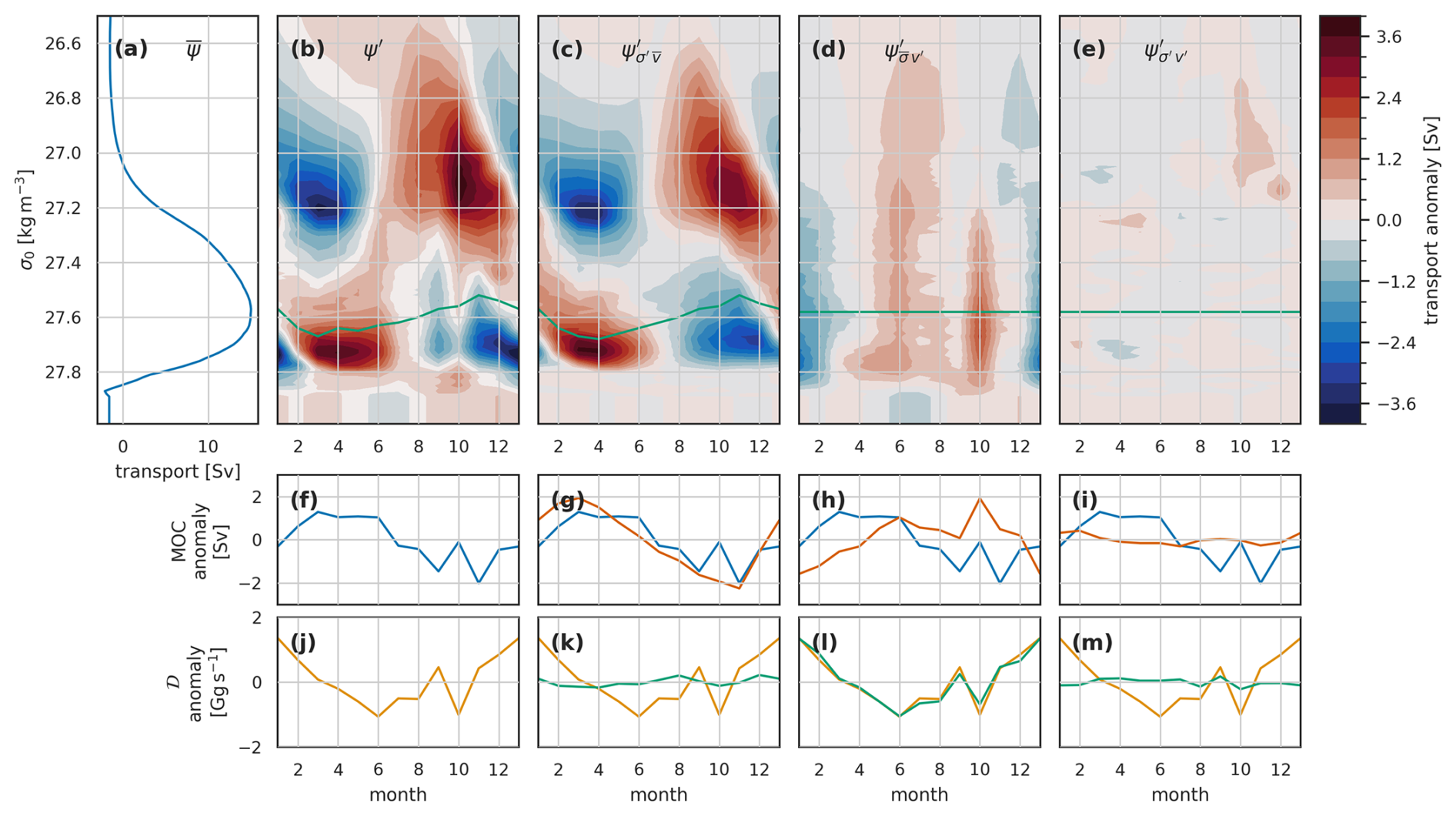
Figure 4 The seasonal cycle in the overturning streamfunction (Ψ), MOC, and density flux (𝒟) for the full OSNAP transect in the Viking20x model. (a) The mean overturning streamfunction. (b–e) Hovmöller (time – σ) plots of seasonal streamfunction anomalies. The green line in each shows the associated variability of σ_MOC. The plots are arranged in columns: (b, f, j) the full anomalies, (c, g, k) the anomalies associated with density variations and mean velocities, (d, h, l) velocity variations and mean density, and (e, i, m) velocity and density covariation. The lower two rows are MOC (f–i) and density flux 𝒟 (j–m). In (g–i), the blue line is for the total anomalies, copied across from (f), while the orange line is the respective anomaly component. Similarly, the yellow total anomaly line in (j) is repeated in (k–m) alongside the green line showing the respective components of the density flux anomaly.

If we consider, for example, March in Fig. 4c, we see negative anomalies at densities peaking at 27.2 kg m⁻³. Looking at Fig. 5a, the 27.2 kg m⁻³ isopycnal is present only in the eastern basin, and Fig. 5b and c show the density anomalies to be confined to the near-surface. Thus, the negative March streamfunction anomaly is the result of winter cooling in the predominantly northward-flowing surface waters. We find very little, if any, lighter-than-average waters in March, so the positive anomaly between 27.5 and 27.8 kg m⁻³ must be due to denser-than-average southward-flowing water. Southward-flowing waters in this density range are found in the East Greenland and Labrador Sea currents Fig. 5a. For the full OSNAP section, the East Greenland Current anomalies largely cancel out the northward flow just downstream in the West Greenland Current, so the positive March density-driven streamfunction anomalies (Fig. 4c) are largely due to seasonal denser waters flowing south in the Labrador Current.

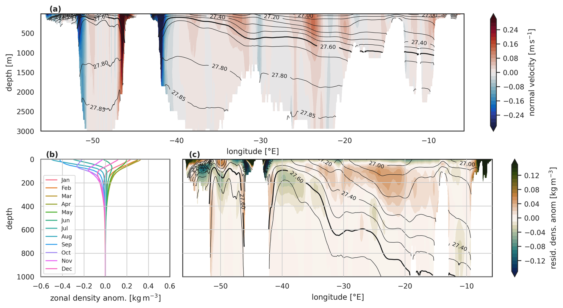
Figure 5 (a) Shading shows the long-term mean northward velocity normal to the OSNAP section in the Viking20x model; the long-term mean potential density contours are overlaid. The σ₀=27.6, i.e. the approximate mean σ_MOC, contour is highlighted. The strong boundary currents in the west are clearly seen, as is the deepening of the density contours toward the east. (b) Seasonal cycle of model zonal-mean monthly density anomalies. Note that the zonal mean seasonal density variability is largely confined to the surface 200 m and almost entirely confined to the surface 500 m. The maximum positive seasonal anomalies (densest surface waters) are found in March–April at all depths; the maximum negative anomalies (lightest waters) are found between August and December depending on the depth. The deeper layers lag behind the surface layers in seasonal minimum densities. (c) Shading shows the remaining density anomalies, after the zonal mean anomalies are removed, for March, when surface waters are at their densest. Notice the smaller amplitude of these remaining anomalies compared to the zonal mean anomalies. The zonal mean March anomalies would take the form of strongly positive anomalies on this plot, so red colours here are areas where the zonal mean underestimates the spring density maximum and green colours are where the zonal mean is an overestimate.

The velocity-driven anomalies (see Fig. 4d) are perhaps simpler to understand. Positive anomalies, such as those observed in June, result from stronger-than-average northward flow (or weaker-than-average southward flow) of light water, which must be combined with stronger-than-average southward flow (weaker northward flow) of dense water. Lighter waters are generally found at the surface or in the east. Thus, positive velocity-driven anomalies could due to stronger northward (weaker southward) surface velocities balanced by adjustment of the return flow at depth or due to stronger, more barotropic flow northward in the east and southward in the west, for example, an increased subpolar gyre. The final plot on the top line of Fig. 4e shows residual anomalies associated with covariation of the density and velocity and is always small.

The remaining line in Fig. 4b–d, i.e. the green line, shows the monthly evolution of σ_MOC. The streamfunction anomaly along this line is (very nearly) the MOC anomaly plotted below in Fig. 4f–i. From the position of this line in density space, relative to the streamfunction anomalies, we see that the total and density-driven seasonal MOC variability is largely driven by the variability at higher densities, that is, by the seasonal density variation, near-surface, in the southward-flowing Labrador Current. The velocity variability drives little change in σ_MOC.

The final row of panels, i.e. Fig. 4j–m, shows the density flux, which is the −1 times the integral in density of the anomalies, i.e. the integral from top to bottom of the panels b–e. Here, we see that when integrated, the dipole structure, which dominates the density-driven anomalies, results in very little density flux – that is, while the shape of the streamfunction curve changes seasonally with density variability, the area beneath remains fairly constant. In contrast, the velocity variability dominates the density flux because, although the associated anomalies are small compared to the density-driven ones, they maintain a consistent sign across the full density range.

Using the above guidance to interpret Fig. 4, we see that the monthly overturning streamfunction anomalies (${\mathrm{\Psi }}_{\mathit{\sigma }}^{\prime }(\mathit{\sigma },m)$, Fig. 4b) have a dominant dipole structure in both density and time. At lower densities (less than about 27.4 kg m⁻³), positive overturning streamfunction anomalies peak in autumn, with negative anomalies peaking in spring. Conversely, at higher densities (greater than 27.4 kg m⁻³), positive streamfunction anomalies peak in the spring, with negative anomalies peaking in autumn. While the density of maximum overturning also varies through the year, with a maximum in spring when waters are densest after winter cooling and a minimum in autumn, it always lies within the higher density range. Hence, the seasonal cycle in MOC_σ (Fig. 4f), which approximately samples the anomalies at density σ_MOC (green line in Fig. 4b), samples the higher densities resulting in the spring maximum and autumn minimum in MOC_σ. The density flux (Fig. 4j) shows the maximum southward density flux (largest negative values) in June and minimum in January, lagging 2–3 months behind the meridional overturning seasonal signal.

We now decompose the overturning streamfunction anomalies into separate parts driven by seasonality in density and velocity (Eq. 21, Fig. 4c–e). The dipole structure occurs in the anomalies associated with density variability (${\mathrm{\Psi }}_{{\mathit{\sigma }}^{\prime }\stackrel{\mathrm{‾}}{v}}^{\prime }(\mathit{\sigma },m)$, Fig. 4c). The seasonal cycle at lighter densities, with its peak in autumn, is caused by the seasonal cycle in density of northward-flowing water. The cycle is reversed for denser waters, with peak positive overturning streamfunction anomalies in spring; we discussed above how this is due to these denser surface waters flowing predominantly southward. The seasonal velocity variability drives a different pattern of overturning streamfunction variability, with a consistent sign across almost the whole density range (${\mathrm{\Psi }}_{\stackrel{\mathrm{‾}}{\mathit{\sigma }}{v}^{\prime }}^{\prime }(\mathit{\sigma },m)$, Fig. 4d). This annual cycle has its minimum in January and peaks in July, with a secondary sharp peak in October. This pattern corresponds with an increase in net northward flow of lighter waters in phase with a net southward flow of denser waters.

The resulting seasonal variability in the meridional overturning (Fig. 4f–i) is mostly due to the seasonal density variation (Fig. 4g) and, in particular, the seasonal density variation of denser waters. The velocity variation acts mostly to delay the MOC seasonal peak and introduce some higher-frequency variability in autumn. In contrast, the seasonal northward density flux anomalies (Fig. 4j–m) are almost entirely due to the velocity variability (Fig. 4l).

Decomposing the overturning streamfunction further, beginning with the velocity-driven component (Fig. 6), we find the dominant factor to be the seasonal cycle in surface Ekman transport. This produces seasonal overturning streamfunction variability, with a maximum in summer and a minimum in winter. The timing is due to the surface Ekman transport being generally southward, opposing the overturning. The summer maximum corresponds to a minimum in this opposition. The streamfunction variability shows as a summer MOC maximum and northward density flux minimum (i.e. southward maximum). The remainder again shows a narrow peak overturning streamfunction anomaly in autumn; we have been unable to discover the precise cause of this, but it appears to be located in the barotropic transport variability. The shorter 6-year model results show a stronger seasonal cycle driven by the barotropic velocity variability (Fig. S1c in the Supplement), suggesting interannual variability of the seasonal cycle.

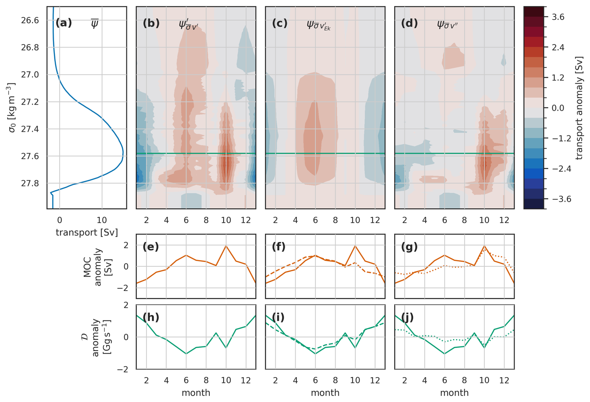
Figure 6 The seasonal cycle due to velocity variability (constant mean density structure) in the overturning streamfunction (Ψ), MOC, and density flux (𝒟) for the full OSNAP transect in the Viking20x model. (a) The mean overturning streamfunction. (b–d) Hovmöller (time – σ) plots of seasonal streamfunction anomalies. The green line in each shows the associated variability of σ_MOC. The plots are arranged in columns: (b, e, h) the full velocity-driven anomalies, (c, f, i) velocity-driven anomalies associated with Ekman surface velocity variability, and (d, g, j) anomalies associated with the remainder of the velocity variability. The lower two rows are MOC (e–g) and density flux 𝒟 (h–j). In (f, g), the solid orange line is for the total velocity-driven MOC anomalies, copied across from (e); the dashed line in (f) is the Ekman-driven MOC anomaly, and the dotted line in (g) is the remainder-driven MOC anomaly. Similarly, the solid green total density flux anomaly line in (h) is repeated in (i, j) alongside the dashed line in (i) showing the Ekman-driven 𝒟 and the dotted line in (j) showing the remainder-driven 𝒟 anomaly.

Turning to the density-driven component, we decompose this in two independent and complementary ways: first, separating out the component associated with the zonal mean seasonal cycle of density, and second, separating into two components due to temperature and salinity variations. The zonal mean seasonal cycle of density is almost entirely confined to the surface 500 m (Fig. 5) and accounts for almost all the density-driven variability in MOC and most of that in the overturning streamfunction (Fig. 7). The domination of the zonal mean density signal in MOC variability is due to the seasonal cycle of summer/autumn lighter surface densities and winter/spring denser surface waters in the near-surface southward flow. This southward flow occurs primarily in the East Greenland Current and Labrador Current. Because much of the East Greenland Current flows back northward as the West Greenland Current, much of that transport cancels out, leaving the OSNAP-wide seasonal MOC variability largely dominated by near-surface density changes in the Labrador Current.

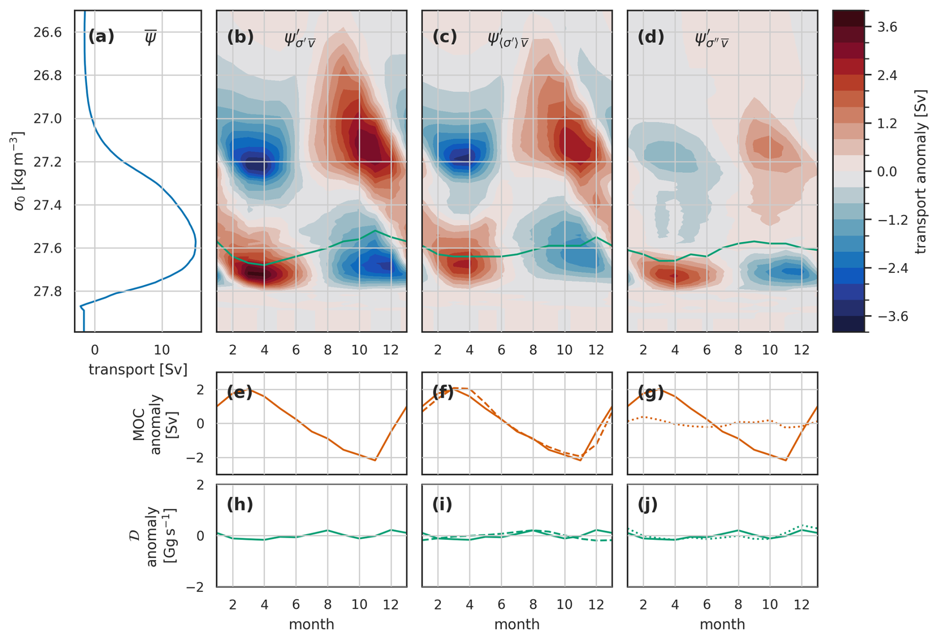
Figure 7 Similar to Fig. 6 but for the seasonal cycle due to density variability (constant mean velocity structure) in the overturning streamfunction (Ψ), MOC, and density flux (𝒟) for the full OSNAP transect in the Viking20x model. This figure has the same structure as Fig. 6, but the columns here refer to (b, e, h) the full density-driven anomalies, (c, f, i) density-driven anomalies associated with zonal mean density variability, and (d, g, j) anomalies associated with the remainder of the density variability.

The variability in the density-driven streamfunction remainder (Fig. 7d) has the same pattern as that associated with the seasonal zonal mean density variation (Fig. 7c) but with lower amplitude, suggesting that the zonal mean annual density signal is underestimating the annual signal in both lighter northward flows (σ<27.4 kg m⁻³) and denser (σ>27.6 kg m⁻³) southward flows. Figure 5c confirms this, with dense anomalies present in March in the widespread near-surface northward flow (15–30° W, surface 200–400 m) and also in the strong southward flow below 300 m on the Labrador coast. These remainders have little expression in the MOC because of the density at which they occur. The two effects largely cancel out in the density flux metric. This cancellation appears to be by chance for the full OSNAP section and does not hold for the separate OSNAP_E and OSNAP_W calculations below. Note that the isopycnal depth change in the Labrador Current outflow is the only notable seasonal influence we see on the overturning streamfunction in the model from below 500 m – here, down to 800–1000 m. Some seasonal deep density variation in the Rockall Trough can be seen, but it is in a region of low velocity, so it does not impact the overturning streamfunction.

Finally, we examine the separate contributions of seasonal temperature and salinity variability to the density-driven seasonal cycle (Fig. 8). The seasonal cycle in the overturning streamfunction is dominated by temperature variability, responsible for the dipole pattern in both density and time. The influence of salinity variability is mostly confined to the upper limb, where σ<27.6 kg m⁻³ (Fig. 8b–d). While the seasonal cycle in the overturning streamfunction seasonal variability is dominated by temperature, both MOC and density flux seasonal cycles have fairly equal amplitude contributions from temperature and salinity variability (Fig. 8f, g, i, and j). For MOC, sampling the streamfunction at the maximum (green line in Fig. 8b–d) does not capture the maximum temperature-driven anomaly, and integrating the anomalies in density space for the density flux involves cancellation of the large positive and negative temperature-driven anomalies (Fig. 8c, f, and i). However, the overall smaller-amplitude salinity-driven streamfunction anomalies, with a single peaked form in density, are more efficiently expressed in both MOC – where the streamfunction anomaly occurs at densities including σ_MOC – and density flux – as there is no cancellation of anomalies when integrating in density space (Fig. 8d, g, and j).

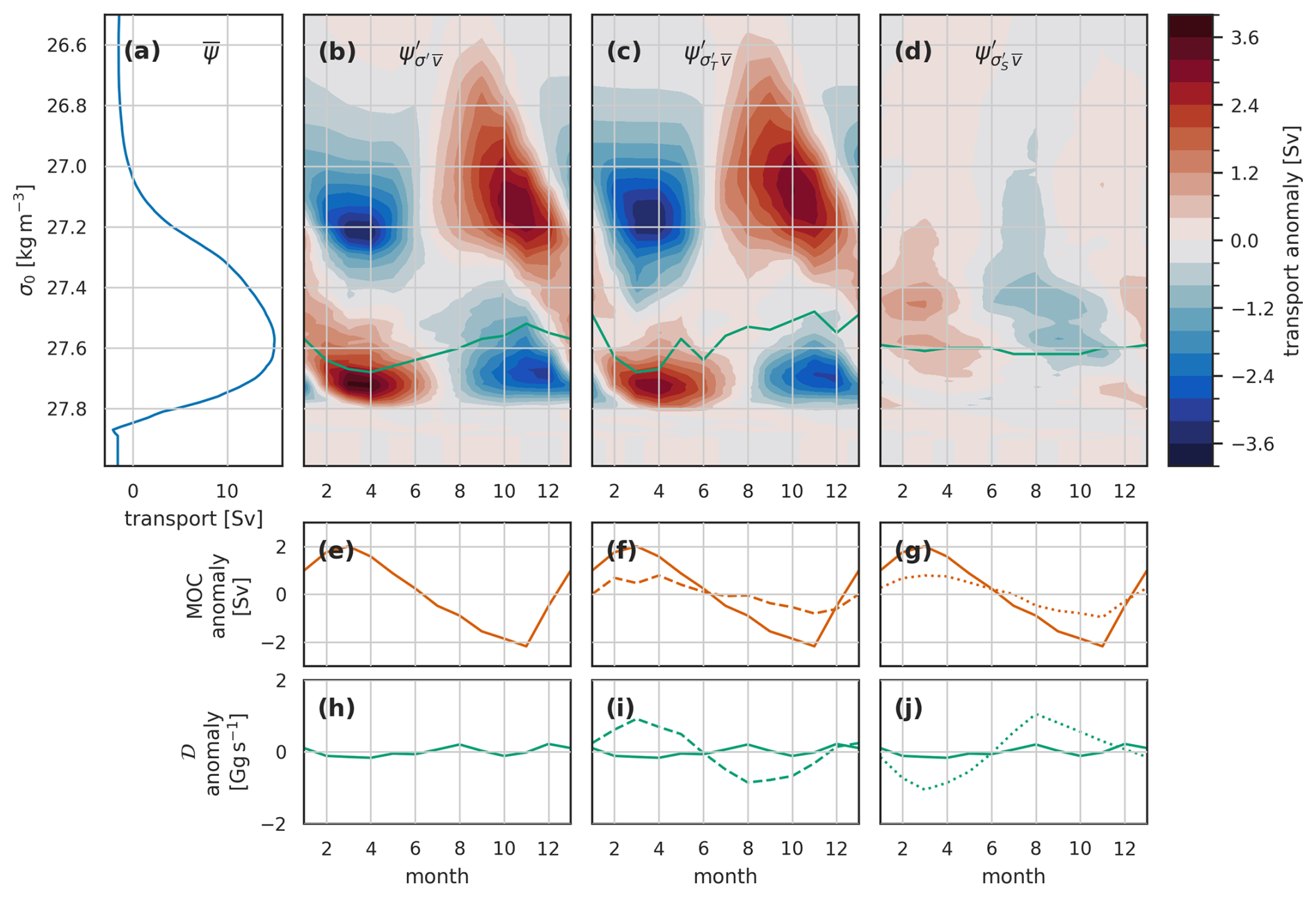
Figure 8 Similar to Fig. 7 but for the decomposition of the seasonal cycle due to density variability into separate components driven by temperature and salinity variability. This figure has the same structure as Fig. 7, but the columns here refer to (b, e, h) the full density-driven anomalies, (c, f, i) density-driven anomalies associated with temperature variability, and (d, g, j) anomalies associated with salinity variability.

Interestingly, while temperature and salinity contributions to MOC are in phase – both with a spring maximum and an autumn minimum – the contributions to density flux are out of phase, with temperature variability producing a spring maximum in northward density flux (minimum southward) and salinity variability showing a spring maximum in southward density flux. Naively, we might expect both stronger MOC and more southward density flux when overturning is larger; this is what we observed in the velocity-driven component described above and in the salinity-driven component here. In the temperature-driven component, the phase relationship between density flux and MOC is reversed. As for the total density-driven MOC above, the temperature-driven seasonal MOC is dominated by the southward-flowing water in the western boundaries, whereas the density flux seasonality is dominated by the larger streamfunction variability at lower densities associated with northward surface flow in the eastern basin.

The salinity-driven streamfunction cycle (Fig. 8d) appears to be the result of two regional seasonal cycles in surface salinity. There is slight winter freshening due to excess precipitation over evaporation across the interior and east of the basin. This tends to reduce density, in opposition to cooling increasing density, and results in the largely opposite phase of salinity- and temperature-driven streamfunction variability where σ<27.4 kg m⁻³. At the western boundaries, particularly in the shallow shelf regions, a salinity minimum occurs in late summer due to freshwater input from ice melt. These coastal waters are still part of the upper limb but flowing southward, so this autumn salinity and density minimum produces negative streamfunction anomalies. We look at this in more detail when discussing OSNAP_E and OSNAP_W separately below.

To aid comparison with the seasonal cycles of MOC and density flux for OSNAP_E and OSNAP_W and in the OSNAP observational data, we bring together the MOC and density flux plots from Figs. 6–9.

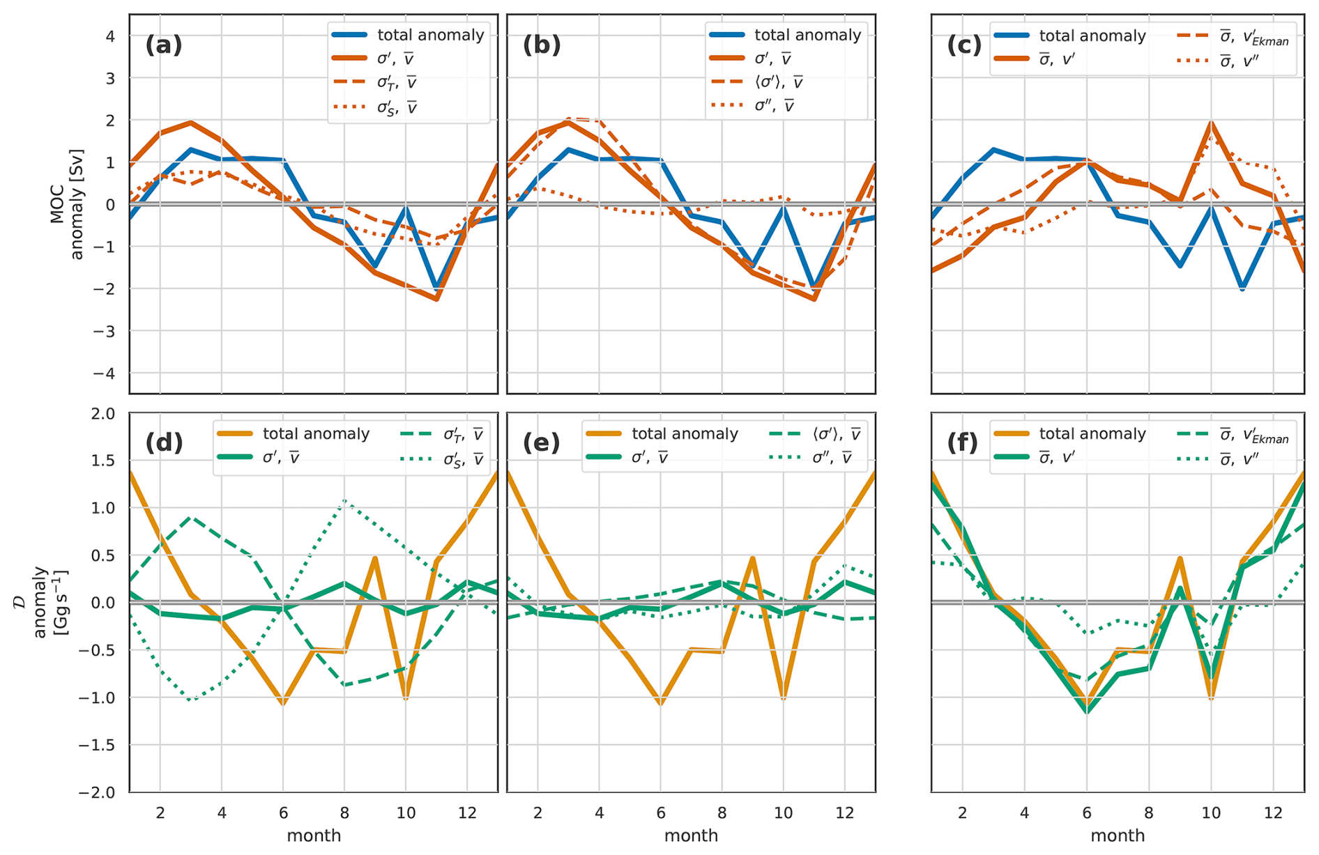
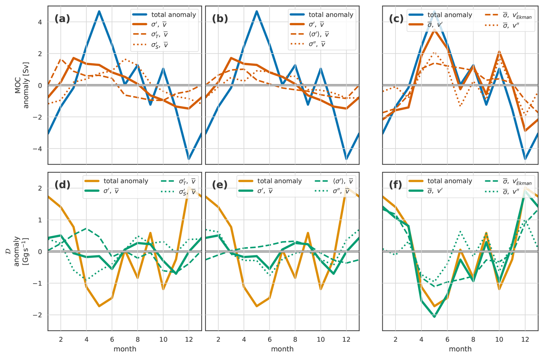
Figure 9 Summary plot of the decomposition of the seasonal cycle for the full OSNAP section of (a–c) MOC_σ and (d–f) density flux 𝒟 for the Viking20x model. The left-hand column (a, d) shows the density-driven decomposition into temperature and salinity components; the middle column (b, e) the density-driven decomposition into the zonal mean and remainder components; and the right-hand column (c, f) the velocity-driven decomposition into the Ekman and remainder components. The blue line repeated in (a–c) is the total MOC_σ anomaly; the solid orange line is either the total density-driven anomaly component of MOC_σ (a, b) or the total velocity-driven component (c). The dashed and dotted lines in (a–c) are, respectively, (a) the temperature- and salinity-driven components; (b) the zonal mean density and density-driven remainder components; and (c) the Ekman-driven and velocity-driven remainder components. Similarly, for (d–f), the repeated yellow line is the total 𝒟 anomaly; the solid green line is either the total density-driven anomaly component of 𝒟 (d, e) or the total velocity-driven component (f). The dashed and dotted lines in (d–f) are, respectively, (d) the temperature- and salinity-driven components; (e) the zonal mean density and density-driven remainder components; and (f) the Ekman-driven and velocity-driven remainder components. Several of the subsequent figures share this format, so it is worth spending a moment to understand it.

3.1.2 OSNAP east and OSNAP west

Due to space constraints, we do not show the full streamfunction anomalies individually for OSNAP_E and OSNAP_W. However, the fundamental structure of the anomalies is the same for the partial sections as for the full section: the overall anomalies are dominated by the dipole structure in seasonal density-driven anomalies, while the velocity-driven anomalies have a simpler seasonal cycle with a coherent sign across the full density range. The main differences between OSNAP_E and OSNAP_W streamfunction anomalies is in the densities, where the maxima and minima are positioned. At OSNAP_E, the lower-density anomalies, associated with northward flow, are as much as for the full section. The higher-density anomalies, associated with southward flow, now in crossing OSNAP_E in the East Greenland Current, occur at lower densities than for the higher-density anomalies in the full section, which we attributed to the Labrador Current. This reflects the further densification of waters within the Labrador Sea. For OSNAP_W, the anomalies at lighter densities associated with northward flow closely mirror the dense OSNAP_E southward flow anomalies. This finding supports the idea of notable “cancellation” of East and West Greenland Currents when the full section is considered. The denser OSNAP_W anomalies closely resemble the dense anomalies in the full section.

The resulting seasonal cycles of MOC and density flux in the individual OSNAP_E (Fig. 10) and OSNAP_W (Fig. 11) sections bear many similarities to those in the full section (Fig. 9). In all cases, the seasonal cycle of the overturning circulation, MOC, is dominated by the component due to density variation – specifically by the seasonal cycle of density in the southward surface flow at the western boundary. The Ekman contribution is largely confined to OSNAP_E, which is due to the orientation of the prevailing wind vectors eastward parallel to OSNAP_E (driving surface flow southward across the section) but perpendicular to OSNAP_W (driving along-section flow, which does not contribute to overturning).

Figure 10 Same as for Fig. 9 but for the Viking20x model seasonal cycle at OSNAP_E.

Figure 11 Same as for Fig. 9 but for the Viking20x model seasonal cycle at OSNAP_W.

Perhaps the most notable difference between the full OSNAP section and both OSNAP_E and OSNAP_W is that while the density-driven seasonal density flux anomalies across OSNAP were small (Fig. 9d and e), they are a significant factor in the seasonal cycles at both OSNAP_E and OSNAP_W. The OSNAP_E and OSNAP_W density fluxes cancel when considering the full section. This cancellation is largely explained by variability associated with the East Greenland Current flowing southward across OSNAP_E being strongly correlated with that of the West Greenland Current flowing northward across OSNAP_W.

OSNAP_E, compared to the full OSNAP section (Fig. 9), shows more domination of both MOC and density flux seasonal cycles by temperature variability (Fig. 10a and d), with the salinity component confined almost entirely to OSNAP_W. OSNAP_E seasonal temperature variability is also the source of the slightly counter-intuitive result where enhanced MOC is associated with weaker southward density flux.

For OSNAP_W, as for the full section, temperature- and salinity-driven seasonal variability reinforce each other for MOC but are opposed for density flux (Fig. 10a and d). OSNAP_W is the only region where the salinity signal dominates, at least for the density flux. The timing of the salinity-driven density-flux cycle, its domination by OSNAP_W, the density of the associated largest streamfunction anomalies (Fig. 8), and the domination of all the seasonal cycles by near-surface variability point to the salinity-driven part of the seasonal cycle of overturning at OSNAP being largely driven by the seasonal cycle of salinity in the shallow coastal part of the Labrador Current.

In the full section, the decomposition of density-driven variability into the zonal-averaged seasonal cycle and a remainder (Fig. 7) produced no net contribution from the remainder to either MOC or density flux, though variability was seen in the residual streamfunction (Fig. 7d). We showed (Fig. 5) that this residual streamfunction variability is made of two spatially separate contributions: the contribution at lighter densities is due to the seasonal cycle in the North Atlantic Current in the eastern part of OSNAP_E, while the contribution at higher densities is due to the seasonal cycle of density deeper in the Labrador Current outflow across OSNAP_W. The contribution from the remainder term to the density-driven density flux is now split between OSNAP_E and OSNAP_W, resulting in the larger, opposing contribution of density-driven anomalies to the seasonal cycle of density flux in OSNAP_E and OSNAP_W when compared to the full OSNAP section.

It should be noted that while the density fluxes in OSNAP_E and OSNAP_W sum to the full OSNAP density fluxes, the same does not hold for MOC, as σ_MOC is significantly denser in OSNAP_W than in OSNAP_E.

3.2 Observed seasonal cycles

3.2.1 Full OSNAP section

The mean seasonal cycle of the overturning streamfunction (Fig. 12a) in the observations is very similar to the model (Fig. 4a), though with the peak overturning at a slightly higher density.

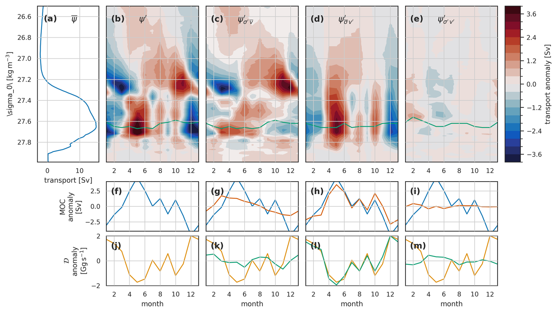
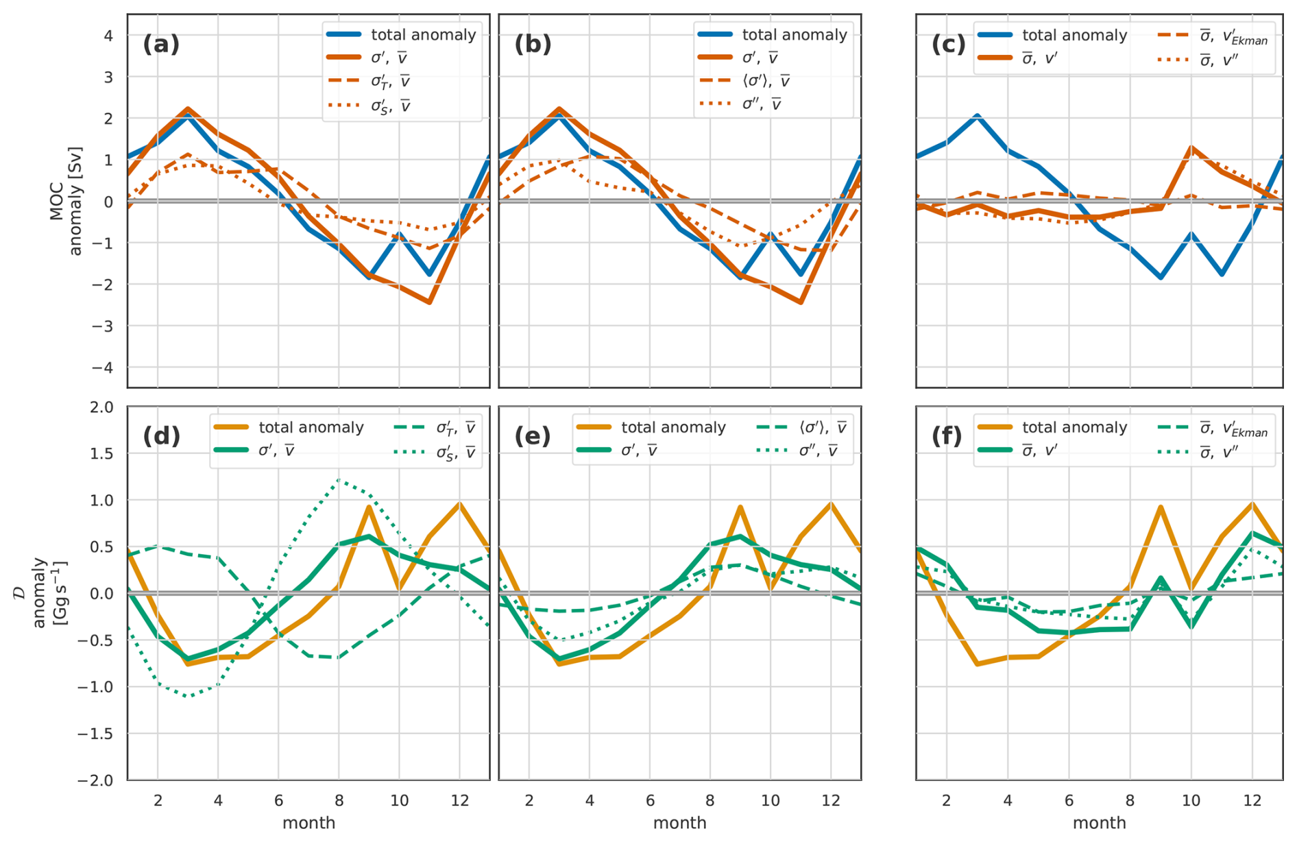
Figure 12 The seasonal cycle in the (a–e) overturning streamfunction Ψ, (f–i) MOC, and (j–m) density flux 𝒟 for the full OSNAP transect in the OSNAP observations. Seasonal total anomalies (b, f, j) are decomposed into (c, g, k) density-driven, (d, h, l) velocity-driven, and (e, i, m) co-varying density-velocity components. See Fig. 4 for full details of the figure layout.

Comparing the observed seasonal cycle of the streamfunction (Fig. 12b–d) with the model (Fig. 4b–d) highlights many similarities but also notable differences. Perhaps the most noticeable difference is the higher levels of high-frequency (month-to-month rather than seasonal) variability in the observations compared to the model. This high-frequency signal is dominated by the velocity-driven component. This disparity is partly due to the shorter time period analysed in the observations (6 years as opposed to 20 years in the model). To test this, we repeated the model analysis using only the 2014–2020 period to match the observations. While this produced a larger high-frequency signal than the 20-year model run, it was still notably smaller than that in the observations. A subset of these 6-year model results are presented; see Figs. S1–S3 in the Supplement.

Looking past this high-frequency signal to the seasonal signal, we again see the dipole structure described in the model (Fig. 12b), though not as well-defined. At lower densities, this is dominated by the density-driven anomalies (Fig. 12c) and, in particular, by the zonal mean near-surface density-driven anomalies (not shown). At higher densities, above and around the density of maximum overturning, this density-driven seasonal cycle (Fig. 12c) is somewhat weaker in the observations than in the model.

The velocity-driven anomalies are stronger in the observations (Fig. 12d) than in the model (Fig. 4d), with a particularly strong maximum centred in May, which is not really present in the modelled anomalies. This May maximum is mostly in the residual component and is part of the higher-frequency signal described above.

The generally weaker density-driven and stronger velocity-driven seasonal cycles in the observed overturning streamfunction are reflected in the meridional overturning (Fig. 12f–i) and density flux (Fig. 12j–m). Whereas in the model, the density-driven component was the largest component of MOC_σ, in the observations, the velocity-driven component dominates both MOC and the density flux.

Figure 13 breaks down the observed MOC and density flux into the various components (compare with Fig. 9). The observed MOC seasonal cycle, in contrast to the model, is dominated by the velocity-driven anomalies. These anomalies are a combination of the annual cycle of surface Ekman-driven flows, with a minimum in the winter when the stronger wind-driven Ekman currents oppose the overturning, and residual flows. The Ekman-driven seasonal variability is larger in the observations than in the model, which is largely due to the different time periods covered. The 6-year model results (Figs. S1–S3), covering the same period as the observations, show a larger-amplitude Ekman component than the 20-year model run, more in line with the observations, suggesting that this may be a result of interannual variability in the seasonal cycle of the winds. The residual flows, generally showing higher-frequency variability, are notably larger in the observations than in the model. The density-driven part of the observed MOC seasonal cycle, as for the model, shows contributions from both temperature and salinity variability (Fig. 13a), though the observed variability due to salinity is shifted out of phase (lagging by 4–5 months). The density-driven MOC variability (Fig. 13b) has a larger contribution from the residual component than in the model.

Figure 13 Same as for Fig. 9 but for the observed seasonal cycle in the full OSNAP section.

The observed density flux seasonal cycle, as with the model, is dominated by the velocity-driven variability (Fig. 13f), though with a generally larger contribution from both the residual and Ekman components than in the model. The density-driven component of the observed density flux seasonal cycle is relatively small and variable, with no clearly dominant components (Fig. 13d and e). As for the model, the observed density flux seasonal cycle shows some opposition between temperature and salinity-driven signals.

3.2.2 OSNAP east and OSNAP west

For OSNAP_E, as for the full section, velocity-driven variability dominates both MOC and density flux seasonal cycles (Fig. 14). This velocity variability is a combination of seasonally varying Ekman transports and a high-frequency remainder. Though it forms the smaller part of the seasonal cycle, we look now at the density-driven variability in more detail.

Figure 14 Same as for Fig. 9 but for the observed seasonal cycle at OSNAP_E.

A particular feature of the seasonal cycle of observed density-driven MOC in OSNAP_E, which is not seen in the full OSNAP section, OSNAP_W, or the model, is the opposing contribution of temperature and salinity (Fig. 14a). We examine this in Fig. 15, where we plot the difference between the early spring and early autumn extremes of the seasonal cycle.

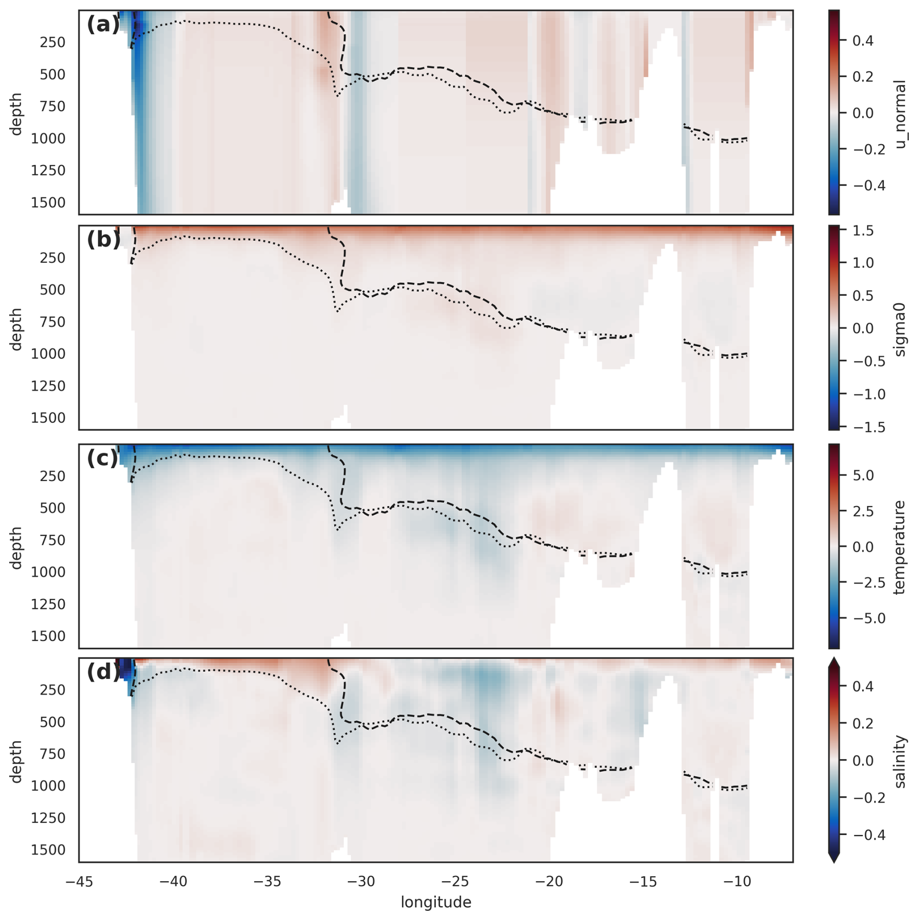
Figure 15 Observed OSNAP_E density-driven seasonal cycle. (a) Mean velocity normal to the section, with σ_MOC for April (dashed line) and October (dotted line) superimposed. These represent the observed extremes of the density-driven seasonal cycle of σ_MOC. (b, c, d) show the difference between water properties in April and October (shading, April–October) for (b) density, (c) temperature, and (d) salinity. The σ_MOC for April (dashed line) and October (dotted line) are superimposed in each case.

Evaluating Eq. (18) at σ=σ_MOC, we see that the density-driven part of the seasonal cycle of MOC is entirely due to the seasonal cycle of the depth of σ_MOC (z^′(σ_MOC)). In particular, we see how σ_MOC depth variability, which is a function of location (x), interacts with the local mean velocity field. This implies that, in Fig. 15a, the difference in density-driven MOC between these two seasonal extremes is purely due to the transport by the mean currents in the region between the respective σ_MOC isopycnals. Thus, we find the seasonal cycle of density-driven MOC in OSNAP_E to be almost entirely due to seasonal changes in the near-surface density in the Irminger Basin, as elsewhere the seasonal vertical migration of σ_MOC is small. The resulting seasonal cycle in MOC, with a spring maximum and an autumn minimum, is the result of a competition between the eastern Irminger Basin, where northward mean transports drive a spring minimum and an autumn peak in MOC, and the East Greenland Current in the western Irminger Basin, where southward mean transports drive a spring peak and an autumn minimum. The resulting density-driven seasonal cycle is dominated by the cycle in the East Greenland Current.

The dominant feature of seasonal density variation on OSNAP_E, Fig. 15b, is the basin-scale, near-surface seasonal cycle described earlier. This seasonal cycle in density produces a strong seasonal cycle in the depth of σ_MOC, and hence large contributions to MOC seasonal variability, in regions where σ_MOC is close to the surface, that is, in the Irminger Sea. The basin-scale surface density signal is primarily driven by large-scale seasonal temperature variation (Fig. 15c). In addition, over much of the Irminger Sea, the seasonal signal of near-surface salinity (Fig. 15d) reinforces the temperature variation, further reducing density in autumn through seasonal freshening. However, Fig. 14a shows the salinity-driven signal to oppose the temperature-driven signal. This opposing salinity-driven signal is due to a small region west of the section where the near-surface seasonal cycle of salinity is reversed (small blue area in Fig. 15d), opposing the temperature-driven signal, with warm salty water present in autumn. This dominates the salinity-driven seasonal cycle because of the strong southward currents. This feature is also present in the model but lies mostly outside the region enclosed by the seasonal variation of σ_MOC. This more detailed analysis of the observed density-driven MOC at OSNAP_E highlights how variability in the MOC measure of meridional overturning can be dominated by very local changes in regions of strong flow.

Observations of MOC and density flux at OSNAP_W (Fig. 16d–f) show a generally smaller amplitude and less coherent seasonal signal than in the model. Velocity variation is dominant, as in all the observations, even with a small Ekman contribution. The observed seasonal cycle of density flux again shows opposing temperature and salinity components as for the observed full OSNAP section and the model. As described previously (Sect. 3.1.1), this opposition of temperature and salinity in the density flux seasonal cycle is due to the temperature component being dominated by the seasonal heating and cooling in northward-flowing surface waters, while the strong seasonal summer freshening of the southward surface flow on the western boundary dominates the salinity component.

Figure 16 Same as for Fig. 9 but for the observed seasonal cycle at OSNAP_W.

3.3 Seasonal cycles of heat and freshwater transport

We might expect, with small net throughflow, that the density fluxes (Figs. 9d–f and 13d–f) would be some form of weighted sum of the heat and freshwater fluxes (with the sign reversed). This relationship is not immediately obvious from the heat and freshwater fluxes for either the model (Fig. 17) or observations (Fig. 18).

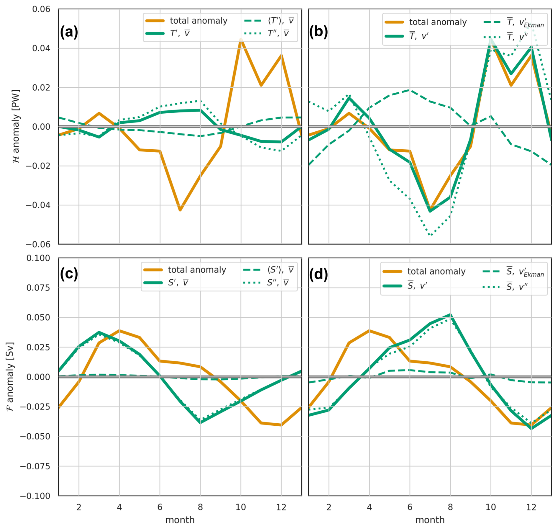
Figure 17 The modelled OSNAP heat transport ℋ (a, b) and freshwater transport ℱ (c, d) seasonal cycles. (a) Seasonal heat transport anomalies driven by temperature variability and mean velocities, presented as follows: solid yellow line – total anomaly; solid green line – total temperature-driven anomaly; dashed green line – component due to zonal mean temperature variability; dotted green line – component due to residual temperature variability. (b) Seasonal heat transport anomalies driven by velocity variability and mean temperatures, presented as follows: solid yellow line – total anomaly; solid green line – total velocity-driven anomaly; dashed green line – component due to Ekman transport variability; dotted green line – component due to residual velocity variability. (c) Seasonal freshwater transport anomalies driven by salinity variability and mean velocities, presented as follows: solid yellow line – total anomaly; solid green line – total salinity-driven anomaly; dashed green line – component due to zonal mean salinity variability; dotted green line – component due to residual salinity variability. (b) Seasonal freshwater transport anomalies driven by velocity variability and mean salinities, presented as follows: solid yellow line – total anomaly; solid green line – total velocity-driven anomaly; dashed green line – component due to Ekman transport variability; dotted green line – component due to residual velocity variability.

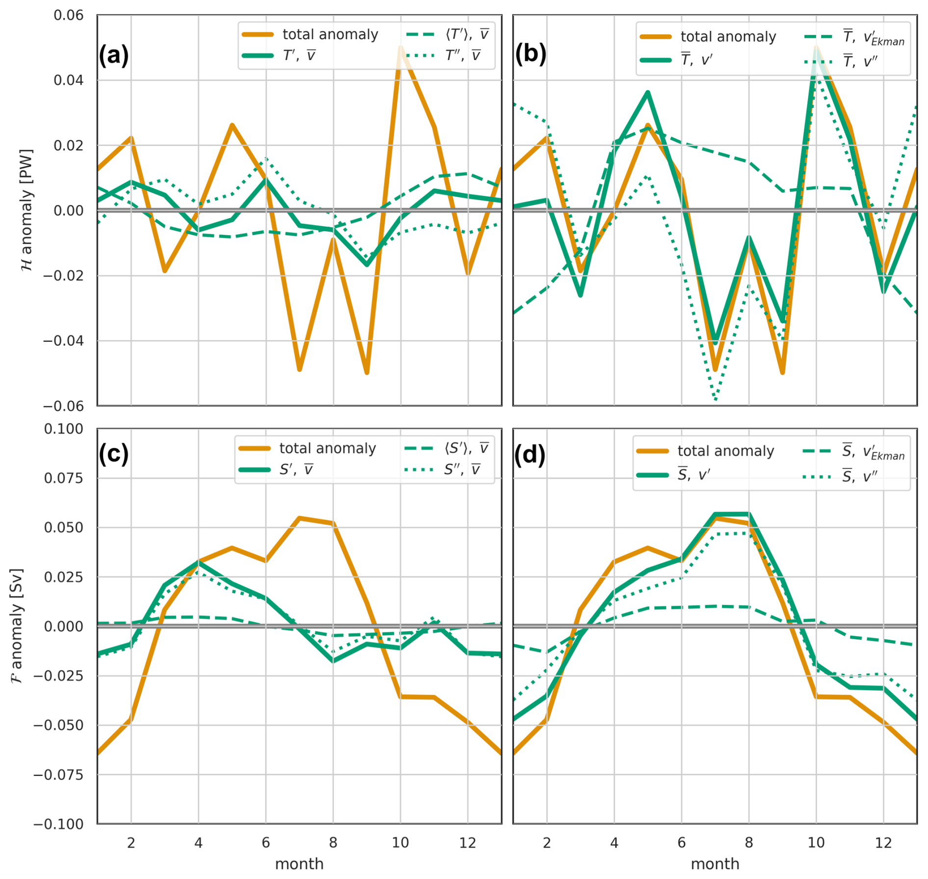
Figure 18 The observed OSNAP heat transport ℋ (a, b) and freshwater transport ℱ (c, d) seasonal cycles. For a full description of the panels, see Fig. 17.

Closer examination suggests that the fundamental shape of the seasonal cycle of the density flux is being dominated by the freshwater flux. Both density and freshwater flux are predominantly southward through the year; the winter minimum and spring-summer maximum in the southward density flux correspond to the winter maximum and spring-summer minimum in the southward freshwater flux. The heat flux plays a more minor role, shifting the peak in the density flux and, particularly in the observational case, adding higher-frequency variability. The principle complicating factor in relating heat and freshwater flux to density flux is the large variability of the thermal expansion coefficient with temperature – at low temperatures, the same amount of added heat causes a much smaller change in density than at higher temperatures.

Examining the decomposition of heat transports into components driven by the seasonal cycle of temperature and velocity (Figs. 17a and b and 18a and b), we find that, as for density flux, the seasonal cycle of heat transports is dominated by the velocity variability acting on the mean temperature field. However, whereas for density flux the dominant velocity variability is surface Ekman, for heat transport the seasonal variability is dominated by the remainder term, predominantly variability in the barotropic flow. In the observations, this barotropic velocity variability is also the source of the high-frequency variability in heat transport. As the driving velocity variability is the same for both heat transport and density flux, the difference in dominant velocity component – Ekman or barotropic – must be due to the interaction between the velocity variability and the mean temperature or density fields.

For freshwater transport (Figs. 17c and d and 18c and d), the seasonal cycle is also, to a large extent, driven by the barotropic velocity variability, with peak southward freshwater transport in winter and a minimum in late summer in both the observations and model. In contrast to the heat transport, for freshwater transport, the property-variability term (here, salinity) also plays a role (Figs. 17c and 18c), having similar magnitude to the velocity-driven term. This shifts the phase of the seasonal cycle of freshwater transport to earlier in the year, with a spring minimum in southward freshwater transport and a late summer/autumn maximum. This phase corresponds to the seasonal cycle of freshwater exiting southward across the OSNAP line in the near-surface western boundary current. Notice that the salinity-driven variability lies entirely in our remainder term – rather than in the zonal-averaged salinity variability. This remainder term contains the horizontal structure of salinity variability. Figure 15d, for OSNAP_E, shows more horizontal structure in salinity variability than for either temperature or density; the same holds true for the full OSNAP section. The strongest seasonal salinity variability is found near-surface in the western boundaries, rather than over the broad zonal horizontal scales. Coupled with the strong currents, this western boundary variability dominates the salinity-driven part of the seasonal freshwater transport signal.

4 Discussion

We have examined the seasonal cycle of subpolar North Atlantic overturning in the overturning streamfunction and four associated metrics: the commonly used meridional overturning, MOC (the maximum of the streamfunction Ψ), heat transport, freshwater transport, and the less commonly considered density flux. We have looked at each of these in an eddy-resolving model and in observational data from the OSNAP array. We have further divided these metrics into separate components driven by velocity and density variability. We have attempted to place these metrics in a coherent framework, particularly highlighting the relationship of the MOC and the density flux to the overturning streamfunction. The main results are summarised in Sect. 5; here, we consider the following questions in a little more depth: is the density flux a useful (additional) metric for monitoring overturning? What may cause the differences between modelled and observed seasonal cycles? How do our results complement and advance previous studies of the seasonal cycles of subpolar overturning? What are the implications, if any, for the monitoring and study of lower-frequency variability of the overturning circulation?

Firstly, we consider the density flux. For the seasonal cycle, each of the metrics considered is dominated by a different physical process or region. For example, for the full OSNAP section seasonal cycle, MOC is mostly responding to a combination of the near-surface density in the western boundary current and Ekman transport variability; density flux is dominated by Ekman transport variability; heat flux is dominated by the variability of non-Ekman, mostly barotropic, residual velocities; and freshwater flux responds to a combination of the barotropic velocities and the seasonal cycle of surface salinity in the western boundary. The density flux may not therefore appear very useful – mostly responding to the Ekman transport variability. However, this is largely due to the cancellation of density-driven seasonality in the density flux between OSNAP_E and OSNAP_W, with temperature variability dominating in OSNAP_E and salinity variability dominating in OSNAP_W. As an integrated measure, rather than an extreme, the density flux is arithmetically “better” behaved than MOC: the averages, sums, trends, and variability of the density flux are simple to calculate. MOC, however, must always be considered in the context of the changing σ_MOC value – for example, the annual mean MOC is not the same as the mean of the monthly MOCs, as each monthly maximum will occur at a different σ_MOC. The MOC metric, at least for the seasonal cycle, is found to be extremely sensitive to density variation in very limited geographic regions – for example, MOC variability in OSNAP_E is found to be dominated by surface temperature variability in the Irminger Basin and the East Greenland Current, where the σ_MOC isopycnal is close to the surface. Meanwhile, the density flux appears to be a more balanced measure, responding to multiple processes across the whole basin. We might even conclude that the current focus of many overturning studies on the Irminger Basin and East Greenland Current is as much a function of the characteristics of the MOC metric as of the importance of these regions to overturning. Density flux turns out not to be a simple combination of heat and freshwater flux; this is highlighted here, as both heat and freshwater flux seasonality are strongly influenced by the barotropic velocity variability, which plays only a minor part in the density flux seasonality. We suggest that density flux complements the more commonly used overturning metrics and as such would recommend that density flux become a routinely used additional metric, if not the primary metric, when studying the overturning circulation.

While modelled and observed seasonal cycles are largely consistent, there are some differences. The observations show a larger Ekman-driven seasonal cycle, which is primarily due to the different averaging periods for the model and observations. When the model analysis is repeated on the observational time period, the Ekman component is correspondingly stronger (Figs. S1–S3). The modelled seasonal cycles of both MOC and density flux show a larger contribution from the density-driven variability than the observations. Some of this is due to a weaker freshwater cycle in the model (the freshwater-driven overturning often opposes the heat-driven overturning), and some to a stronger seasonal cycle of near-surface temperature in the model, particularly in OSNAP_E. This may be a function of the surface forcing dataset used in the Viking20x model or, alternatively, an underestimate of the seasonal cycle of surface temperature in the observations. We have shown how the MOC metric is extremely sensitive to temperature and salinity variability in quite confined regions of strong flow near the surface. Finally, and perhaps the largest difference between model and observational seasonal cycles, there is the presence of high-frequency variability, particularly evident in the non-Ekman-driven velocity component in the observations. This is centred in OSNAP_E and in the barotropic velocities. A small part of this high-frequency variability is due to the shorter period spanned by the observations (see Figs. S1–S3); the rest may be due to missing physics in the model or the difficulty in making high-quality observations of barotropic currents with limited resources.

Observational and modelling studies of subpolar North Atlantic meridional overturning consistently return estimates of the seasonal cycle of overturning, as measured by the maximum of the overturning streamfunction (MOC_σ), with an amplitude of about 4 Sv with a late spring maximum and an autumn or a winter minimum (Lozier et al., 2019; Wang et al., 2021; Fu et al., 2023a; Tooth et al., 2023; Mercier et al., 2024). Our results, both model and observational, confirm these general conclusions.

Published analyses, both model-based and observational, tend to focus on MOC seasonality, predominantly in the eastern subpolar gyre (OSNAP_E and OVIDE). These show the subpolar AMOC seasonal cycle to be dominated by seasonality in the Irminger Basin, particularly the East Greenland Current, modified by Ekman transport driven by seasonality in the zonal winds (Wang et al., 2021; Fu et al., 2023a; Tooth et al., 2023; Mercier et al., 2024). Observational (Le Bras et al., 2018; Mercier et al., 2024) and model (Tooth et al., 2023) analyses find the MOC variability due to the East Greenland Current to be a combination of density-field and transport variability – though it is difficult to disentangle the two due to the dominance of geostrophic currents. The results we obtain generally confirm the importance of Ekman and western boundary processes in the seasonality of MOC. However, we find little contribution from western boundary transports in either models or observations, the western boundary contribution to MOC being almost entirely explained by the zonal mean density variability. This is particularly notable because this zonal mean density variability has no associated zonal pressure gradients, so it is uncoupled from the velocity fields.

The Irminger Basin and East Greenland Current density and transport seasonality have been ascribed to a lagged signal of water mass transformation and North Atlantic deep water (NADW) formation in the Irminger Basin (Fu et al., 2023a), with the relatively short lag time attributed to the travel time from the transformation regions to OSNAP_E (Le Bras et al., 2020; Fu et al., 2023a). However, Tooth et al. (2023) points out that the 4 Sv seasonal signal in overturning is much smaller than the 20 Sv seasonality in the water mass transformation in the Irminger Basin north of OSNAP_E, the difference between the two being seasonal heat storage and release from the surface waters. While we do not disagree with this lagged transformation diagnosis, we note that the seasonality of MOC is tied to the seasonality of the surface density structure, mostly summer/autumn warming and winter/spring cooling. This seasonality naturally lags behind the water transformation cycle, which is tied to the surface fluxes, mostly due to the large heat capacity of seawater and vertical mixing. Given the basin-scale nature of the surface density cycle and the similar large scale of seasonal surface heat fluxes (e.g. Berry and Kent, 2009), the simpler explanation for the seasonal rise and fall of the σ_MOC isopycnal due to the local seasonal cycle of surface fluxes is perhaps more appropriate than that of advectively lagged water transformation. We note that advection certainly has a role in surface flux effects on density, but the estimated seasonal advective distances involved in even the fastest currents in the region (8 months around the northern segment of the Irminger Basin; Tooth et al., 2023) are still relatively small compared to the length scales of seasonal surface fluxes.

We must emphasise that the location of the dominant OSNAP_E overturning seasonality in the East Greenland Current is not new; it confirms the results of Wang et al. (2021), Fu et al. (2023a), Tooth et al. (2023), and Mercier et al. (2024). However, we also emphasise that this local dominance is partly a feature of the MOC metric, as density, heat, and freshwater flux seasonal cycles are less dominated by this single small region. The Irminger Basin and East Greenland Current dominance of the MOC seasonal cycle is due to a combination of two factors – the dominance of the cycle by near-surface seasonal density variability and this region being the only part of OSNAP_E where the σ_MOC isopycnal is within the depth range of this surface density variability (Fig. 15). MOC needs to be carefully interpreted in the context of σ_MOC position and variability.

While these comparisons and the exploration of mechanisms driving the seasonality of the MOC overturning metric are enlightening, the more interesting result is how poorly the MOC metric seasonal cycle predicts the seasonal cycle in any of the integrated metrics – density, heat, and freshwater fluxes – mostly due to its high sensitivity to a small set of processes in a limited geographical region. It is these integrated metrics and how they evolve that are arguably more relevant to understanding the potential changes to overturning seasonality, which are most important for mitigating the impacts of AMOC changes on Atlantic sector weather and climate.

We now consider how our conclusions from analysis of the seasonal cycles may be extended to longer-term monitoring of the Atlantic meridional overturning circulation. The model-observation seasonal cycle differences require consideration from both large-scale overturning observational and modelling perspectives to improve confidence in observations and predictions of overturning. The largest differences found were in the representation of barotropic currents and near-surface seasonal temperature and salinity structures – particularly in the boundary currents – at depths that may be shallower than the upper sensors on long-term monitoring arrays. Both of these differences suggest possible focusses for improvement of long-term AMOC monitoring and climate modelling. Further, MOC is commonly used for climate model verification; however, a focus on reproducing the MOC metric may be a poor guide to the quality of the modelled overturning circulation and property fluxes.

We find the most commonly considered MOC metric – the maximum of the overturning streamfunction – to be overly focussed on seawater property changes in a couple of small geographic regions: flows in the upper 500 m in the East Greenland Current and 1000 m in the Labrador Current. This is certainly the case on seasonal timescales, and it may be a more reliable metric on longer timescales, but this needs to be demonstrated. We also note that while OSNAP_E makes the largest contribution to all the metrics (except freshwater flux), the focus on MOC perhaps exaggerates the comparative importance of OSNAP_E vs. OSNAP_W to the overturning circulation and its wider implications, and within OSNAP_E,MOC probably underemphasises the importance of the northward flows of warm and salty waters in the eastern subpolar gyre (Iceland Basin and Rockall Trough) to the overturning. We need to be mindful of all these characteristics of the MOC metric when designing observational campaigns.

Although extrapolating from the present work on seasonal variability to longer timescales is difficult, the characteristics of the MOC metric seasonal variability – the domination of the metric by movement of a single density interface – are not obviously specific to short timescales. In recent work, Chafik and Lozier (2025) raise similar concerns about the use of the MOC metric, concluding that it essentially captures variability in upper ocean heat content, which can result from a number of mechanisms, some unrelated to overturning. Models of overturning slowdown (see for example Baker et al., 2025) show a combination of reduced volume transformation across the density of maximum overturning (sampled by the MOC metric), the changing density of maximum overturning (often ignored), and a reduced density difference between northward and southward flows (not sampled by MOC). There is a risk that an exclusive, or excessive, focus on MOC in both modelling and observations could underestimate the long-term societally relevant AMOC decline, for example, by missing decline associated with a changing density difference between upper and lower limbs (Koman et al., 2024). The use of the density flux metric alongside MOC could help capture such changes while requiring no additional observations.

Heat and freshwater fluxes must also not be neglected as measures of overturning, though our analysis finds these to be strongly influenced by the barotropic current variability, including large high-frequency variability particularly evident in the observations. These barotropic currents are perhaps the currents with the largest uncertainty in basin-wide overturning estimates. The barotropic velocity component is generally partly composed of a uniform “compensation” velocity applied to control the total transport through the section. While this compensation involves small velocities, it can integrate to several tens of Sverdrups of transport. The compensation velocity problem has been widely considered (Bryden and Hall, 1980; Lee and Marotzke, 1998; Killworth, 2008), though we could find no published literature specific to the OSNAP section. McCarthy et al. (2015) considered the application of the compensation velocity at RAPID, 26° N in the North Atlantic. They find that the application of different compensation velocity structures does not have much impact on the vertical structure of the MOC streamfunction. The zonal structure of the barotropic component may be more important at OSNAP, interacting with larger interior variability in the density structure (see, for example, the different σ_MOC depths between the Irminger and Iceland basins in Fig. 15).

5 Conclusions

We place meridional overturning and density, heat, and freshwater fluxes in a coherent framework. This framework highlights the integral relationship between meridional overturning circulation and property transports, both being functions purely of the overturning streamfunction Ψ. Using this framework, we examine the seasonality observed in overturning and density, temperature, and freshwater fluxes at the OSNAP line in the subpolar North Atlantic. We find MOC seasonal cycles to be dominated by Ekman transports and a large-scale seasonal cycle of the surface density; heat flux seasonal cycles to be dominated by barotropic velocity variability; freshwater fluxes to be dominated by a combination of barotropic velocities and the salinity in the western boundary current; and density fluxes to reflect a broad range of processes. We further show that the standard measure of overturning, i.e. the MOC metric, is a poor predictor, on seasonal timescales, of either density fluxes or the more societally relevant ocean heat and freshwater transports. This is due to each of these metrics responding to different physical processes. The MOC metric, in particular, has very high sensitivity to near-surface physical processes in a limited geographical area. These processes are not necessarily reflective of either the fundamental or most societally relevant characteristics of large-scale overturning. Although extrapolating from the present work on seasonal variability to longer timescales is difficult, there are enough parallels for us to consider that there is a risk that an exclusive focus on MOC could, for example, miss overturning “slowdown” associated with changing density differences between upper and lower limbs. Additionally incorporating the density flux metric would help capture such changes. Our results complement the recent work of Chafik and Lozier (2025), who raise similar concerns about the characteristics of the MOC metric. Hence, we suggest caution in the exclusive use of the standard MOC metric in studies of overturning and recommend the routine use of the density flux as a valuable additional metric.