Combining BioGeoChemical-Argo (BGC-Argo) floats and satellite observations for water column estimations of the particulate backscattering coefficient

As the second-largest carbon reservoir on Earth, the ocean regulates the carbon balance through dissolved and particulate organic carbon (POC) forms. Monitoring carbon cycle processes is key to understanding the climate system. Although most organic carbon in the ocean exists in dissolved form, POC, despite its smaller share, plays a vital role by connecting surface biomass production with the deep ocean and sedimentation processes. POC estimation is achieved by measuring proxies like the particulate backscattering coefficient (b_bp) estimated from satellite observations and in situ sensors, such as the BioGeoChemical-Argo (BGC-Argo) floats. Previous studies have integrated data from BGC-Argo floats and satellite sensors, demonstrating the potential of machine learning models to estimate vertical bio-optical properties within the water column. The approach presented here enhances the estimation within the top 250 m of the water column compared with previous works. The estimations are performed in two distinct regions, the North Atlantic and the Subtropical Gyres, and across several layers within two maximum depth limits of 50 and 250 m. Data from BGC-Argo profiles and the Ocean and Land Colour Instrument (OLCI) sensor are used together to build a training dataset for a random forest model, which is applied with different sets of variables. Additional considerations regarding our datasets include short time criteria for matchups (±24 h) and high spatial resolution. The random forest model shows promising results, especially within the first 50 m in the Subtropical Gyres.

1 Introduction

The ocean covers approximately 70 % of Earth's surface and plays a fundamental role in regulating climate dynamics. It redistributes energy and carbon through a variety of physical and biogeochemical processes. Among these processes, the biological carbon pump facilitates the transfer of CO₂ from the atmosphere to the ocean floor by enabling the production and sinking of particulate organic carbon (POC), which is sequestered in deep-ocean sediments. POC originates from living organic carbon primarily produced by photosynthetic organisms such as phytoplankton, which thrive in the sunlit upper-ocean layers. These organisms require carbon compounds, along with light and nutrients, to survive and reproduce (Falkowski et al., 1998; Siegel et al., 2014). Their presence and abundance reflect the interplay of resources and losses in the environment (Behrenfeld et al., 2006), with populations maintaining daily division cycles even in regions where nutrients appear to be depleted beyond detection limits (Ribalet et al., 2015; Vaulot and Marie, 1999). Quantifying phytoplankton biomass and carbon content is crucial to understanding these ecosystem dynamics and their role in carbon cycling. Chlorophyll-a (chl-a) concentration has traditionally served as a proxy for phytoplankton biomass, but its interpretation is often challenged by physiological photo-acclimation, which alters intracellular pigment levels without necessarily reflecting actual changes in biomass. The particulate backscattering coefficient (b_bp) has been recognized as a stable optical proxy for phytoplankton biomass and carbon content as it is sensitive to the abundance, size distribution, and composition of suspended particles rather than pigment concentration alone (Behrenfeld and Boss, 2006; Graff et al., 2015; Martinez-Vicente et al., 2013). Unlike chl a, which can underestimate biomass in stratified and oligotrophic waters, b_bp remains relatively unaffected by photo-acclimation effects, making it particularly useful for studying carbon fluxes across different oceanic regions and depth layers. The complex interaction between key variables (usually nonlinear) and the limited sampling resolution in dynamic environments, combined with the technical challenges of depth-resolved measurements, contribute to gaps in our understanding of specific marine processes, such as carbon sequestration, nutrient cycling, sedimentation, and ocean–atmosphere CO₂ exchange.

Bio-optical sensors installed on autonomous platforms, such as the Biogeochemical-Argo (BGC-Argo) profiling floats (Claustre et al., 2020), have become a valuable technology for acquiring in situ data on water mass ecological and physical statuses. These sensors can measure the scattering of light in water, which provides information about radiative transfer conditions and the nature and dynamics of suspended particulate matter. The b_bp parameter is an inherent optical property (IOP) of water, and it has been widely recognized as a robust bio-optical proxy for POC (Cetinić et al., 2012; Sullivan et al., 2013). However, b_bp measured by floats can have an uncertainty on the order of 10 %–15 % (Bisson et al., 2019). These uncertainties stem from the instrumental drift, the sensor calibration limitations, and the reliance on manufacturer calibration files rather than sensor-specific calibrations using dark counts. While autonomous platforms provide extensive spatial and temporal coverage, these factors must be considered when interpreting bio-optical data to ensure accuracy and reliability.

IOPs are intrinsic characteristics of water, determined solely by its composition, and are independent of the external light field or the geometrical angle conditions during observations. These properties include absorption, elastic scattering, inelastic processes (such as fluorescence and Raman scattering), and attenuation, which describe how light behaves and propagates through water. IOPs are essential in studying light interactions in aquatic environments, as they reflect the presence of dissolved organic matter, phytoplankton, and suspended particles. The b_bp can be measured by autonomous platforms spread out across the ocean or derived from scatter measurements by onboard satellite sensors, such as the Sentinel-3 Ocean and Land Colour Instrument (OLCI) (https://user.eumetsat.int/resources/user-guides/sentinel-3-ocean-colour-level-2-data-guide, last access: 28 July 2025) (EUMETSAT, 2019; Jorge et al., 2021; Koestner et al., 2024). Designing observational strategies based on combining the two approaches constitutes a fundamental tool for improving knowledge of ocean processes (BGC, 2016).

Several approaches have been developed to estimate POC from optical measurements of water-leaving radiance (L_w) or to link POC to remote-sensing-derived IOPs (Bisson et al., 2019; Evers-King et al., 2017; Loisel et al., 2002; Stramski et al., 2008). However, these methods are designed to estimate parameters at the sea surface, which does not fully capture the complexities of carbon export in the ocean, as numerous vertical processes within the water column significantly influence the carbon cycle. Fusing satellite data with vertical profiles from BGC-Argo floats to extend the measurements of surface bio-optical properties (i.e., b_bp) to several depth layers is performed using the SOCA method in Sauzède et al. (2016, 2020). The initial SOCA2016 method consists of a neural network combining satellite surface estimates of b_bp and chl-a concentrations, matched up in space and time with depth-resolved physical properties derived from temperature–salinity profiles measured by BGC-Argo profiling floats. This method predicts b_bp for 10 different depths in the productive layer. In 2020, the availability of a larger database with new profiles and the opportunity to increase the vertical resolution of model outputs led to the development of the SOCA2020 method. This approach includes additional sea level anomaly (SLA) inputs with information about submesoscale processes; it replaces satellite-derived products (b_bp and chl a) with simple reflectances at several wavelengths and explores machine-learning-based techniques that are efficient at estimating retrievals, in addition to quantifying the uncertainty associated with the outputs. A significant improvement in the b_bp predictions was revealed, especially near the surface layers.

Building on these results, this research proposes an analysis of the b_bp estimation in the upper layers of the ocean surface using the Sentinel-3 Ocean and Land Colour Instrument (S3OLCI). We change the spatial resolution from the 4 km resolution of GlobColour Level-3 merged products ($\mathrm{1}/\mathrm{24}$° at the Equator) used in previous studies to the 300 m full resolution (FR) of the Sentinel-3 OLCI. Additionally, we evaluate the model performance after incorporating OLCI spectral wavelengths as features for b_bp estimation and compare these results with those obtained using GlobColour. Another key aspect of this study is determining whether adding IOPs derived from satellite data (absorption and scattering) improves the accuracy of the b_bp estimation compared with using reflectances alone. Furthermore, b_bp at different depths of the water column is estimated using multi-output models. These multi-output random forest models account for the high correlation between measurements at nearby depths. Finally, there is a comparison of the accuracy of the b_bp estimations at two depth limits, i.e., from the surface to either 50 or 250 m.

2 Data and methods

Data from in situ measurements collected by BGC-Argo floats, along with satellite data from various projects and missions (GlobColour and Sentinel-3 OLCI), are utilized as inputs for machine learning models. We employ three datasets for two different maximum depths – 50 and 250 m. The three datasets are (1) Level-3 multi-sensor products from GlobColour, (2) Level-2 single-sensor reflectances from the Sentinel-3 OLCI processed with the Case 2 Regional Coast Colour (C2RCC) algorithm (Brockmann et al., 2016), and (3) the second dataset plus IOPs derived from the OLCI using the C2RCC processor again.

2.1 Study area

Two regions of the ocean are analyzed, the North Atlantic (NA) within latitudes 35–80° N and the Subtropical Gyres (STG) with the latitude band 15–40° N/S (Fig. 1). These two areas exhibit distinct seasonal patterns throughout the year, experiencing significant differences in terms of nutrients, light availability, minimum and maximum temperature regimes, mixed layer depth (MLD) variations, thermocline levels, and mesoscale dynamics. One of the main differences between these two regions is the variability in the stratification of the upper-ocean layers. This phenomenon determines the resistance of the water to overturning, thus conditioning the supply of nutrients from deeper waters (Lozier et al., 2011). NA waters are seasonally high in chl a (mg m⁻³). During winter, a weakly stratified upper-ocean water column overturns or mixes, facilitating the upwelling of nutrients needed to sustain surface productivity. In the STG region, spanning thousands of kilometers across the oceans, nutrients are in short supply and waters range from ultra-oligotrophic (chl a ≤ 0.04 mg m⁻³) to oligotrophic (chl a ≤ 0.07 mg m⁻³) (Letelier et al., 2004). During the summer and winter cycles, there is expansion and contraction of their spatial coverage (Leonelli et al., 2022). Despite these extreme nutrient limitations, molecular clock studies have shown that phytoplankton in these regions continue to divide daily, suggesting that microbial communities have adapted through efficient nutrient recycling, regenerated production, and physiological acclimation strategies (Vaulot, 1995; Ribalet et al., 2015). Feucher et al. (2019) showed that the two Northern Hemisphere subtropical gyres have qualitatively very similar stratification structures, with permanent pycnoclines in the North Atlantic and North Pacific.

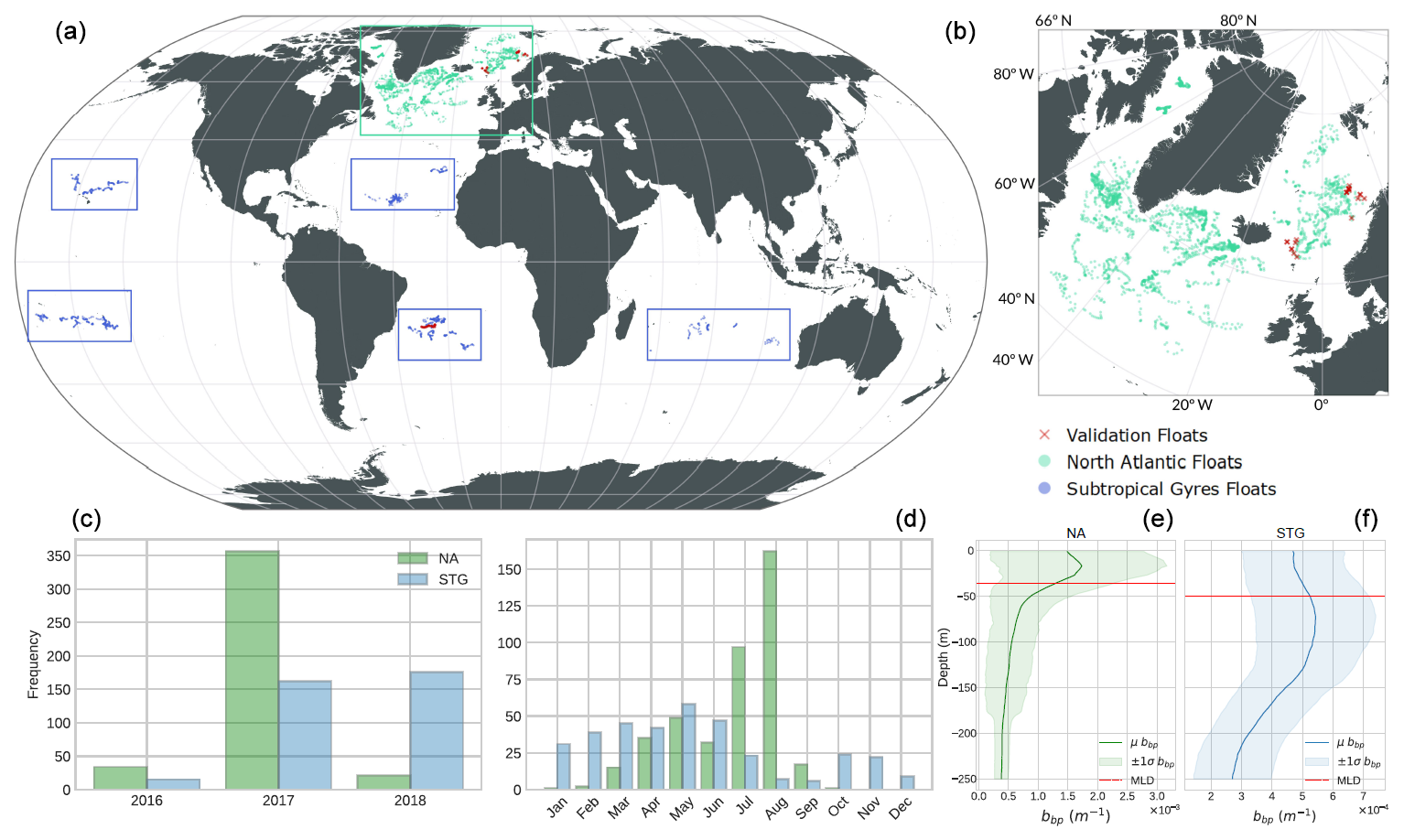
Figure 1 Global map showing the geographic locations of the BGC-Argo floats and satellite data matchups (a, b). Temporal coverage of matchups by year (c) and month (d) for the North Atlantic (NA, green) and Subtropical Gyres (STG, blue). Vertical profiles (e, f) of bbp from floats, where the solid lines show the mean values, the shaded areas show the 1 standard deviation, and the dashed red line shows the average mixed layer depth (MLD).

These regional differences in physical and biological characteristics are also reflected in the vertical distribution of the b_bp, with the NA exhibiting higher surface variability and deeper gradients compared to the more stable stratification of the STG (see Fig. 1). The NA, with its seasonal mixing and higher productivity, generally exhibits higher b_bp values due to increased particulate matter and phytoplankton-derived organic material in the water column. In contrast, the STG, characterized by strong stratification and lower phytoplankton biomass, show significantly lower b_bp values indicative of reduced particle concentrations. Despite the global coverage of the sampled STG regions, there is much more heterogeneity in the NA observations, making it a more complex and challenging environment for modeling purposes, as observed in the results.

The temporal distribution of the matchups shows a clear seasonal bias, with most data concentrated between May and September, particularly during 2017. This uneven distribution is primarily due to the limited availability of the cloud-free satellite observations required to match BGC-Argo profiles, especially during the winter months, when cloud cover and low solar angles reduce the quality of remote sensing products.

2.2 BGC-Argo data

The international One-Argo program provides continuous ocean observations through an array of profiling floats, each equipped with sensors tailored to specific objectives: Core-Argo (for temperature and salinity measurements), BGC-Argo (for biogeochemical measurements), Deep-Argo (for measurements deeper than 2000 m), and Polar-Argo (for measurements in polar environments). Key bio-optical variables, such as chlorophyll a, optical particulate backscattering, and irradiance, can be measured using BGC-Argo profiling floats. These variables are essential for generating products that support biogeochemical and ecosystem studies (Claustre et al., 2009, 2020). The BGC-Argo floats can collect measurements from 1000 m to the surface with a depth resolution of ∼ 1 m every 10 d, even though in many cases the vertical resolution is poorer.

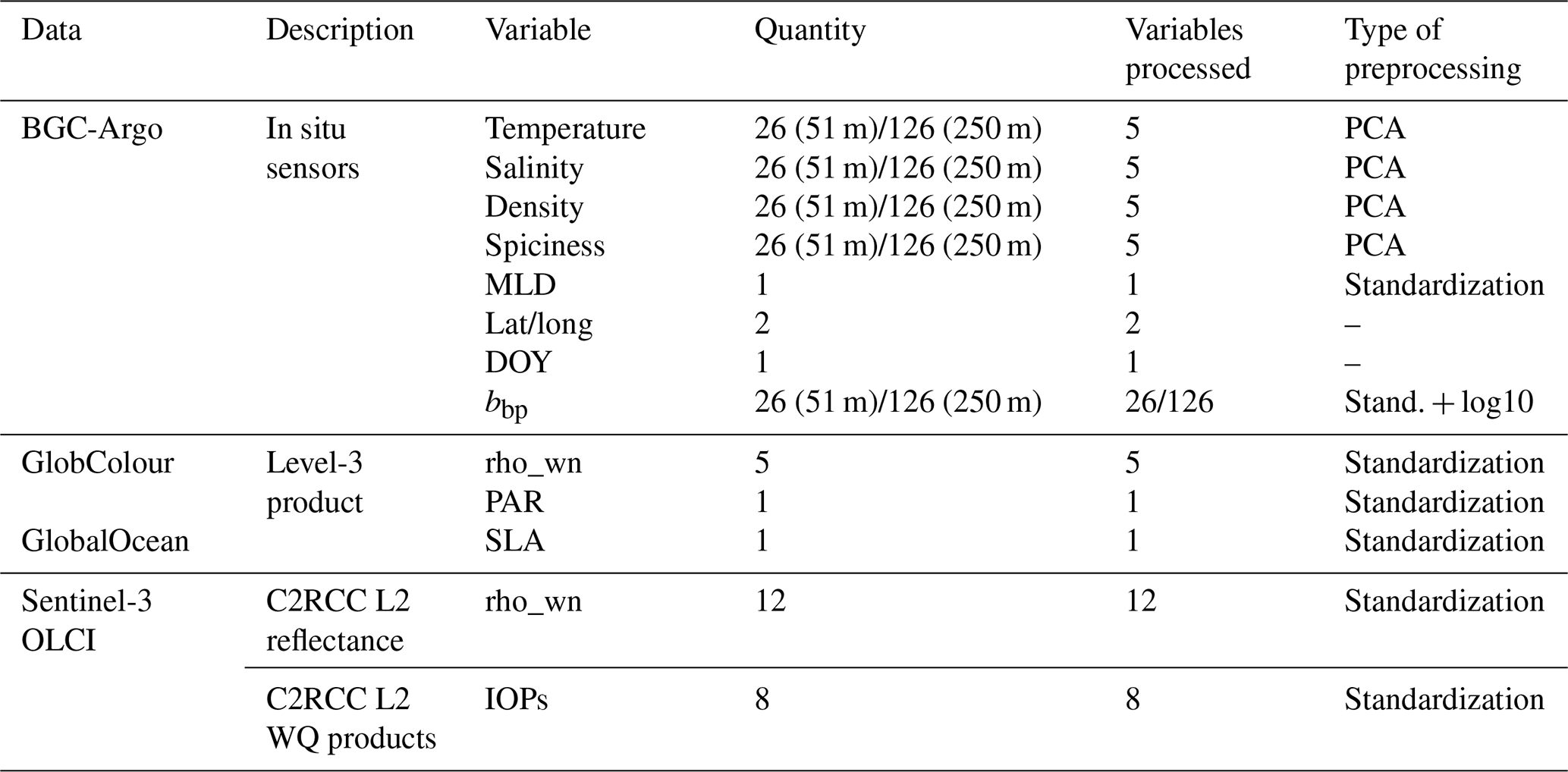
The lower boundary of the euphotic zone is defined as the depth where 1 % of the photosynthetically available radiation (PAR) penetrates the water column (Kirk, 1976). While it is true that phytoplankton growth is ultimately driven by absolute photon flux rather than a relative threshold (Sverdrup, 1953; Behrenfeld and Boss, 2017), the 1 % PAR definition remains a widely used metric for characterizing the physical light environment across diverse oceanographic conditions. This definition focuses on describing the light field as a physical property rather than directly linking it to biological responses, providing a consistent measurable boundary for analyzing water column dynamics. While recent studies have demonstrated that phytoplankton can grow at light levels significantly below this threshold or even under polar night conditions (Randelhoff et al., 2020), our physical optics approach allows for standardized comparisons of light attenuation patterns across our datasets. This depth varies in the global ocean from ∼ 20 m to more than 120 m, depending on the region and season. The flux of sinking carbon that exits the euphotic zone due to gravity is a key component of the overall carbon sequestration budget (Siegel et al., 2014). In the present experiments, a depth limit extending beyond the lower boundary of the euphotic zone (250 m depth) was selected. From 250 m to the surface, measurements of temperature, salinity, density, and spiciness were taken every 2 m, along with information on the MLD – calculated as the depth at which the density exceeds 0.03 kg m⁻³ relative to the density at 10 m (de Boyer Montégut et al., 2004). Vertical measurements of b_bp at the same vertical resolution are also available in the datasets. Spiciness reflects density-compensated variations in temperature and salinity, providing a tracer for water mass origins and mixing processes (Smith and Ferrari, 2009). Since particle concentrations and optical properties often differ between water masses, spiciness anomalies can be associated with variations in b_bp. Warmer and saltier waters (higher spiciness) can boost stratification, reducing vertical nutrient fluxes and potentially limiting biological production, leading to lower concentrations of organic particulate matter and thus lower b_bp. Table 1 shows the different types of variables used to train and validate the proposed models for the designed experiments.

Table 1 Overview of the datasets and variables used in the study. BGC-Argo data include geophysical and bio-optical profiles: temperature, salinity, density, spiciness, mixed layer depth (MLD), particulate backscattering coefficient (b_bp), and geolocation and day of year (DOY). The satellite products comprise remote sensing reflectance (rho_wn), photosynthetically active radiation (PAR), sea level anomaly (SLA), and inherent optical properties (IOPs). Sentinel-3 OLCI data include Level-2 outputs from the Case 2 Regional Coast Colour (C2RCC) processor, including both the rho_wn and water quality (WQ) products. The preprocessing steps included principal component analysis (PCA), standardization, and log10 transformation.

The b_bp value (Mignot et al., 2014) used here is calculated following the work of Sullivan and Twardowski (2009). The angular distribution of scattering relative to the direction of light propagation θ at the optical wavelength λ is known as the volume-scattering function (VSF – β(θ,λ) (m⁻¹, sr⁻¹). It is composed of the sum of pure seawater β_sw and particles β_p, where β_sw depends on temperature and salinity and is calculated using a depolarization ratio of 0.039 (Zhang et al., 2009). The contribution of β_p to the VSF is calculated by subtracting the contribution of β_sw from β(124°,λ):

$$\begin{array}{}\text{(1)}& {\mathit{\beta }}_{\mathrm{p}}(\mathrm{124}\mathit{°},\mathit{\lambda })=\mathit{\beta }(\mathrm{124}\mathit{°},\mathit{\lambda })-{\mathit{\beta }}_{\mathrm{sw}}(\mathrm{124}\mathit{°},\mathit{\lambda }).\end{array}$$

Then, a conversion factor χ with a value of 1.076 for an angle of 124° relates b_bp to β_p, making it possible to extrapolate the measurement from a single angle (124°) to the total coefficient as follows (Boss and Pegau, 2001; Sullivan and Twardowski, 2009):

$$\begin{array}{}\text{(2)}& b_{\mathrm{bp}}\left(\mathit{\lambda }\right)=\mathrm{2}\mathit{\pi }\mathit{\chi }\left(\mathit{\beta }\right(\mathit{\theta },\mathit{\lambda })-{\mathit{\beta }}_{\mathrm{sw}}(\mathit{\theta },\mathit{\lambda }\left)\right).\end{array}$$

The backscattering sensor of the BGC-Argo floats measures β(124°, λ) with λ=700 nm. The quality control procedure carried out is the one followed in the SOCA2016 method.

2.3 BGC-Argo and satellite matchup databases

The matchup database created for the SOCA2020 experiments, which links the BGC-Argo floats to the GlobColour and GlobalOcean data, was utilized in this study. The GlobColour data consist of normalized water-leaving reflectances (rho_wn) at five wavelengths (412, 443, 490, 555, and 670 nm) as well as the PAR product. These rho_wn values are derived from a combination of sensors that constitute the GlobColour product: SeaWiFS, MERIS, MODIS Aqua, VIIRS NPP, and the OLCI (Garnesson et al., 2019). The GlobalOcean set provides SLA data, calculated relative to a 20-year mean of sea surface height and generated with altimeter data from various missions (HY-2A, Saral/Altika, CryoSat-2, Jason-2, Jason-1 T/P, ENVISAT, GFO, and ERS1/2) (CMEMS, 2022). In the cited work, the matchup with BGC-Argo floats was performed using the values from the closest available pixels within a ±5 d window and on a 5×5-pixel grid. Further details of the procedure can be found in Sauzède et al. (2020).

The BGC-Argo measurements used here were matched with Sentinel-3 OLCI data using the Calvalus tool developed by Brockmann Consult GmbH (Fomferra, 2011). The spatiotemporal approach applied consists of a time window between the BGC-Argo profiles and the satellite measurements of ± 24 h, and the spatial satellite coverage around the profile is 3×3 macro-pixels at full-resolution imagery (300 m pixels). Once the matchup between the satellites and floats is established, a baseline quality control is applied to ensure that the satellite-measured reflectances maintain radiometric consistency. First, a flag-based filter is applied, discarding pixels near or under probable cloudy conditions. This is followed by an outlier removal based on a z score ($z=(x-\mathit{\mu })/\mathit{\sigma }$) applied at the macro-pixel level band by band. Then, a coefficient of variation in the 560 nm band ($\mathrm{cv}=\mathit{\sigma }/\mathit{\mu }$) is applied (Bailey and Werdell, 2006). Coefficient values under 0.2 ensure good spatial homogeneity (Ahmed et al., 2013; Hlaing et al., 2013; Zibordi et al., 2009). Finally, the median of the pixels left by macro-pixels is used (Hu et al., 2001), which is a standard procedure in studies focused on oceanic waters (Barnes et al., 2019). These criteria reduced the dataset from the original 4115 matchups to 763 matchups. Specifically, 411 and 352 data points are available for the NA and STG regions, respectively. We excluded data from two floats to be used exclusively for validation purposes: in the NA, the float with unique WMO (World Meteorological Organization) no. 6902545 – with 22 measurements – and in the STG region float WMO no. 3902125 – with 28 measurements – constitute the independent dataset in the validation process.

The selected Sentinel-3 OLCI bands extend from 400 to 753 nm (bands 1 to 12) of normalized water-leaving reflectances (rho_wn). The extraction is done on Level-2 data atmospherically corrected with the C2RCC processor (Brockmann et al., 2016). C2RCC relies on an extensive database of simulated water-leaving reflectances and related top-of-atmosphere radiances, with neural networks trained to perform inversions for both the atmospheric correction and the in-water quality parameter estimation. C2RCC provides parameters like the absorption and scattering of the different constituents (IOPs) at 443 nm, i.e., absorption of chlorophyll pigments (apig), yellow substances (agelb), and detritus (adet) and scattering of particulate matter (bpart), white scatterers (bwit), and additive atot and btot. It also provides total suspended matter concentration, chlorophyll-a concentration, and apparent optical properties (AOPs) like K_d (the diffuse attenuation coefficient). Each parameter has its associated error estimation. From the 25 parameters calculated by C2RCC, we selected the eight mentioned IOPs, plus the reflectance for bands 400 to 753 nm.

2.4 Data preprocessing

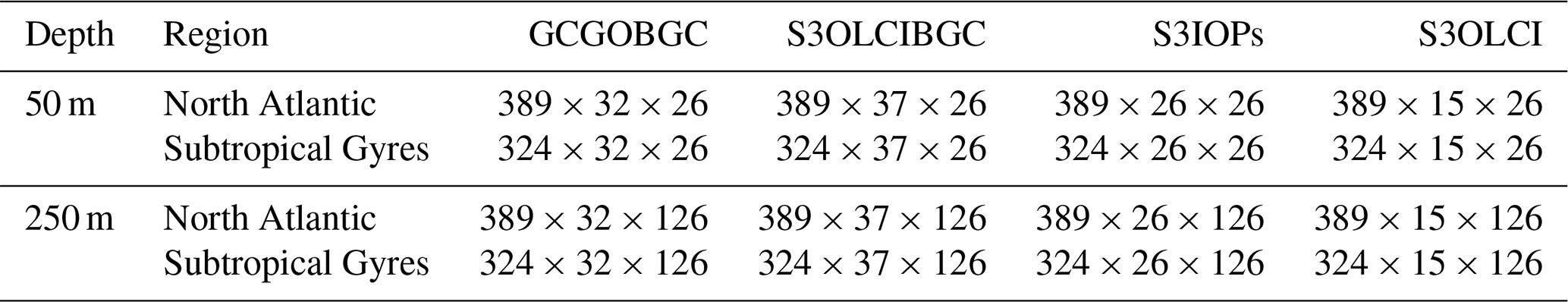
The set and number of parameters (measured or derived) available for the experiments are presented in Table 1. The dataset names in the table correspond to the specific features: GCGO refers to the GlobColour–GlobOcean L3 satellite reflectance combined with the PAR and SLA products (7 features), BGC denotes the Argo-BGC data after preprocessing (27 features across 26 or 126 layers, depending on the depth of 50 or 250 m, respectively), S3OLCI includes 12 reflectance bands, and S3IOPS includes the reflectance bands plus the eight C2RCC-derived IOPs. After excluding the measurements for validation, the two areas have a total of 713 inputs. The maximum number of input variables is 37. The sizes of the matrices can be seen in Table 2. Due to the heterogenous nature of the input variables (X) used to train the models and the high dimensionality and covariance of the variables measured along the water column by BGC-Argo floats, the data were preprocessed to reduce redundancy and multicollinearity. The high-dimensional non-independent variables (temperature, salinity, density, and spiciness) were the ones with the most significant numbers of features. Each variable had one measurement every 2 m, which means 126 measurements in the first 250 m or 26 measurements in the 50 m depth profiles.

Table 2 Dimensions of the input matrices used in the analysis of each dataset, region, and depth. The matrix dimensions are specified as $\mathrm{samples}\times \mathrm{features}\times \mathrm{outputs}$. The datasets include GlobColour and GlobalOcean paired with BGC-Argo (GCGOBGC), the Sentinel-3 OLCI paired with BGC-Argo (S3OLCIBGC), the Sentinel-3 OLCI with IOP products (S3IOPs), and Sentinel-3 OLCI reflectance (S3OLCI).

To reduce the high dimensionality and simplify the regression models, principal component analysis (PCA) is applied to some of the input features. After this feature reduction of the high-dimensional variables, the 250 and 50 m measurements with 126 and 26 inputs are reduced to five components for each variable, resulting in a total of 20 features. This method still retains 99 % of the information. In addition, satellite-derived variables and the MLD were normalized using z-score standardization, i.e., removing the mean (μ_x) and dividing by the standard deviation (σ_x) of each feature.

A second preprocessing step consisted of a logarithmic transformation to the b_bp values measured by the floats. This compresses the dynamic range of the data, which is typically higher near the surface and decreases exponentially by several orders of magnitude with depth. The transformation reduces the influence of extreme values, particularly near the surface, and helps to stabilize the variance across the profiles. As a result, the distribution becomes closer to the Gaussian, which facilitates the training and improves the robustness of the regression models. Finally, variables that consider the spatiotemporal domain, like latitude, longitude, and date (day of year), are also included.

2.5 Multi-output machine learning models

There are two main approaches to dealing with multi-output regression problems. One way is to use univariate models, also known as problem transformation methods (Schmid et al., 2022; Borchani et al., 2015). These methods decompose the multi-output regression problem into multiple single-target problems, creating an independent model for each output. The predictions from these separate models are then combined. This approach ignores the relationships between the targets, which can adversely affect the prediction's overall accuracy. Alternatively, multivariate models are designed to capture dependencies and interactions between the outputs, potentially leading to more accurate predictions (Borchani et al., 2015). When and how to apply these two approaches depends on the nature of the data and the correlation between the targets. In our preprocessing results, PCA decomposition indicates a high covariance among measurements at different depths in the water column. Since our regression models estimate b_bp at different depths, it is logical to consider that nearby values in the water column are related to each other.

A random forest regressor (RFR) (Breiman, 2001) has been widely applied in the geosciences and marine environmental studies for classification and regression tasks (Cutler et al., 2007; Ruescas et al., 2018). Regression trees are at the model's core, which effectively handles complex data when there are nonlinear dependencies between a numerical response variable and a diverse set of predictors, whether qualitative or quantitative (D'Ambrosio et al., 2017). RFR is an ensemble method that combines many weak decision tree learners, which are grown in parallel to reduce the bias and variance of the model simultaneously, enhancing the model's predictive performance. Furthermore, RFR provides insights into the importance of the training features, which reveals the variables that have the most significant impact on the predictions. This capability makes the model's mechanisms and results easier to interpret and explain.

Different algorithms have been tested in previous works (Sauzède et al., 2016, 2020) to estimate b_bp at various depths. Both works are based on a multivariate model applied to all possible outputs. In SOCA16, a multi-layer perceptron is developed, while in SOCA2020 a comparison between a linear model (ridge) and an ensemble model (random forest) is made. The latter showed higher performance. The multivariate RFR used in this study offers higher accuracy than the univariate RFR, especially when the outputs are highly correlated (Schmid et al., 2022) and when complex interactions demand structured inference be effectively managed (Xu et al., 2019). All of the previously mentioned algorithms, including linear regressor (LR), ridge linear regressor (RLR), RFR, and multi-layer perceptron (MLP), were tested at depths of both 50 and 250 m during the dataset preparation phase. The results for 250 m are shown in Fig. 2. Based on these results, the multi-output RFR was selected as the most suitable algorithm for this multi-input or multi-output problem. Results are also analyzed using the built-in feature importance, which is based on the reduction in variance.

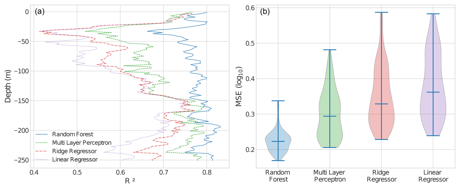
Figure 2 Comparison of different multi-output regression models for estimating vertical profiles of b_bp up to 250 m depth. (a) Depth-resolved R² values for four regression models: random forest, multi-layer perceptron, ridge regressor, and linear regressor. (b) Violin plots of the mean squared error (MSE, log ₁₀-transformed) distributions for each model.

3 Performance of the random forest regressor

Several dataset combinations were used as inputs for the RFR (described in Sect. 2.3). For all of the combinations, the RFR was trained on 80 % of the data, with the remaining 20 % set aside for testing. Experiments were conducted in the NA and STG regions for 26 layers in the range 0–50 m and for 126 layers in the range 0–250 m. The test dataset was exclusively used to evaluate model performance and was never exposed to the regressor during training. For each regression model, we analyzed the key features that contributed to improving the estimation of b_bp in the different combinations. The models were finally validated using two independent floats in the NA and STG regions.

3.1 S3OLCIBGC: results with BGC-Argo and OLCI data

The equivalent set of data from the SOCA2020 experiment (GCGOBGC) is included in the statistical analysis to facilitate a comparison between our findings and previous studies. Tables 1 and 2 present the input features and matrix sizes for the different experiments. In the following sections, we analyze the results of the RFR model applied to these datasets, starting with the GCGOBGC and S3OLCIBGC datasets to establish a baseline. In the NA region, 311 data points are used for training and 78 for testing, while in the STG region 259 data points are used for training and 65 for testing. The results represent 20 % of the dataset used for model testing.

3.1.1 Shallow waters: from 0 to 50 m depth

The performance of the models trained to estimate b_bp in the upper 50 m of the water column is summarized in Fig. 3 and Table 3. Figure 3a includes the depth-resolved R², mean absolute error (MAE), and model bias, while panels (b) and (c) show measured and predicted b_bp profiles, along with relative error distributions for the NA and STG, respectively. Feature importance for both regions and models (GCGOBGC and S3OLCIBGC) is presented in Fig. 4.

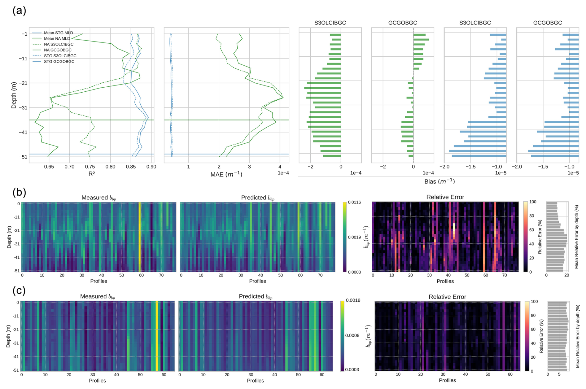
Figure 3 Model performance for estimating shallow-water b_bp profiles (0–50 m). (a) Depth-resolved metrics comparing model predictions using the S3OLCIBGC and GCGOBGC sets as inputs: coefficient of determination (R²), mean absolute error (MAE), and bias. The shaded horizontal lines indicate the average MLD per region. (b–c) Measured and predicted b_bp profiles in NA (b) and STG (c) using S3OLCIBGC. The rightmost bars show the mean relative error by depth.

Table 3 Model performance statistics by region at depths of 50 and 250 m using satellite-based and BGC-Argo data. The metrics reported are the coefficient of determination (R²), median absolute percentage deviation (MAPD; %), and MAE (m⁻¹). The models are based on different input datasets: GCGOBGC, S3OLCIBGC, S3IOPs, and S3OLCI.

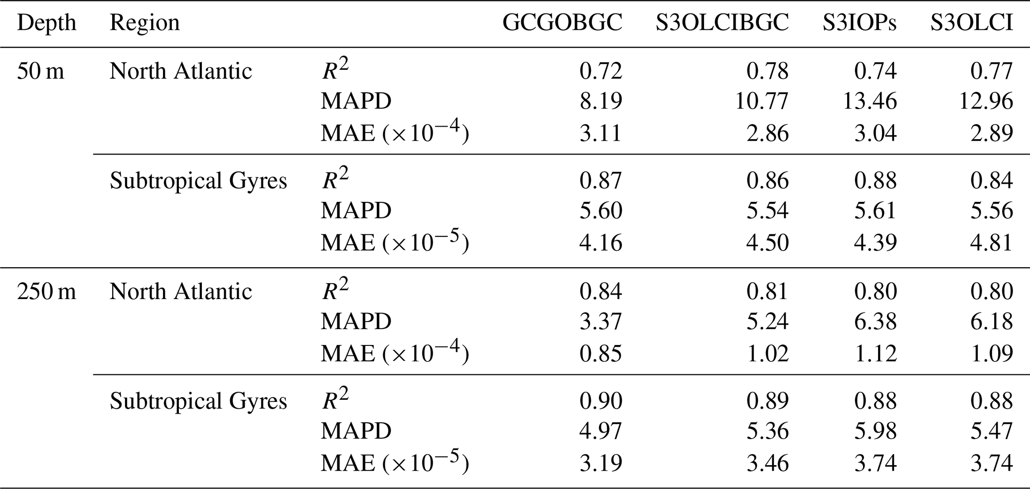
In the NA region (green lines), the S3OLCIBGC model achieves a higher average R² (0.78) compared to the GCGOBGC model (0.72). The MAE is also lower (2.86 $\times {\mathrm{10}}^{-\mathrm{4}}$ vs. 3.11 $\times {\mathrm{10}}^{-\mathrm{4}}$ m⁻¹). In the depth-resolved metrics, the S3OLCIBGC model performs better at both the superficial and deeper layers, maintaining a relatively stable performance down to approximately 20 m. Below this depth, accuracy decreases, particularly across and beneath the average MLD (36 m), where vertical gradients in temperature, salinity, and density intensify and b_bp variability increases (Fig. 1). While the MLD is inherently dynamic and varies throughout the year, this depth represents a critical boundary in our observations, marking a clear threshold where the behavior of the model diverges. The GCGOBGC model shifts from overestimating b_bp in the upper 15–20 m to underestimating values at greater depths. In contrast, the S3OLCIBGC model exhibits a relatively constant negative bias near the surface (1 $\times {\mathrm{10}}^{-\mathrm{4}}$ m⁻¹), which increases gradually with depth, indicating a degradation in the performance of the model. The more balanced contribution of surface and subsurface features in S3OLCIBGC enables the model to better resolve the vertical variability in b_bp below the optical depth. In contrast, the GCGOBGC model presents lower R², higher MAE, and lower MAPD values, all of which indicate a reduced capacity to capture the vertical b_bp variability. These differences likely reflect the superior spatiotemporal fidelity of the S3OLCI matchups (±1 d, 300 m pixels), which enable tighter temporal and spatial coupling between satellite and float observations compared to the broader ±5 d and 4 km of the GlobColour dataset.

In the STG region (blue lines), both models achieve higher performance than in the NA, reflecting the lower variability and more stable vertical structure of b_bp in these oligotrophic waters. The S3OLCIBGC and GCGOBGC models obtain similar results, with mean R² values of 0.86 and 0.87 and MAE values of 4.50 $\times {\mathrm{10}}^{-\mathrm{5}}$ and 4.16 $\times {\mathrm{10}}^{-\mathrm{5}}$ (m⁻¹), respectively. The depth-resolved metrics (Fig. 3) show that the models perform consistently throughout the upper 50 m, with no marked degradation in R² or MAE values near the average MLD (∼50 m). In both cases, the bias remains low in the upper 30 m. However, starting around 35 m, there is an increase in the bias, reaching its maximum near the bottom of the profile.

The feature importance analysis (Fig. 4) shows that latitude is the most relevant feature in this case. This reflects the fact that bio-optical conditions in the STG are very similar throughout the year; the day of year (DOY) is less critical because of the low seasonality in these areas (Mignot et al., 2014; Cornec et al., 2021). The importance of the density and salinity features (Dens_pc1 and Sal_pc1) reflects the barotropic dynamics of these oceanic regions, where isobars and isopycnals are stratified parallel to the ocean surface and vary together as depth is gained (Leonelli et al., 2022).

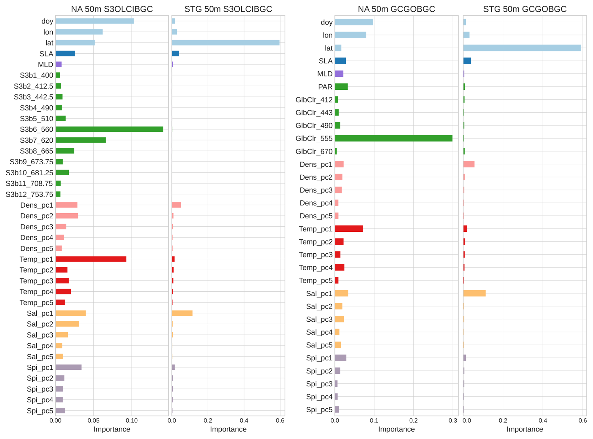
Figure 4 The feature importance (Gini importance) of the models trained with S3OLCIBGC and GCGOBGC to estimate b_bp in shallow waters (0–50 m) in the NA and STG. Features are grouped by category according to color: (1) blue represents the spatial and temporal descriptors, including the day of year (DOY), latitude, and longitude. (2) Dark blue represents the sea level anomaly (SLA). (3) Purple indicates the MLD. (4) Green corresponds to the satellite reflectance bands from either the Sentinel-3 OLCI or GlobColour with its central wavelengths. (5) Pink, red, orange, and light purple correspond to the first five principal components (PCs) derived from the BGC-Argo profiles of density, temperature, salinity, and spiciness, respectively.

3.1.2 Deep waters: from 0 to 250 m depth

The performance of the models to estimate b_bp down to 250 m is summarized in Fig. 5 and Table 3. The S3OLCIBGC and GCGOBGC models obtain R² values of 0.81 and 0.84, respectively, with MAPDs of 5.24 % and 3.37 % and MAEs of 1.02 $\times {\mathrm{10}}^{-\mathrm{4}}$ and 0.85 $\times {\mathrm{10}}^{-\mathrm{4}}$ (m⁻¹). Shallower layers have larger errors in both models and correlate with the observed variability of b_bp with depth in each region. The GCGOBGC does not experience overestimation in the most superficial layers, as was the case for the 50 m models.

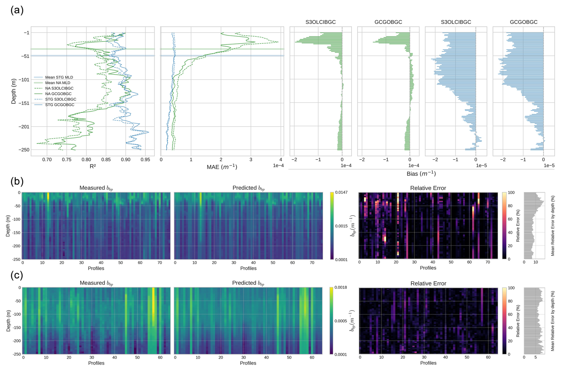
Figure 5 Model performance for estimating deep-water b_bp profiles (0–250 m). (a) Depth-resolved metrics comparing model predictions using S3OLCIBGC and GCGOBGC as inputs: R², MAE, and bias. The shaded horizontal lines indicate the average MLD per region. (b–c) Measured and predicted b_bp profiles in NA (b) and STG (c) using S3OLCIBGC. The rightmost bars show the mean relative error by depth.

Feature importance analyses for both models (Fig. 6) are similar to the 50 m models and also highlight the dominant role of the first principal components (pc1) derived from the BGC-Argo physical variables (density, temperature, salinity, and spiciness). They align with the correlation heatmap (Fig. 6 right), which illustrates how these first PCs correlate with b_bp across depth, showing a strong positive correlation (>0.6) in the 180–250 m range. In these deeper layers, where biogeochemical processes such as particle sinking, remineralization, and carbon export are more active, the relationship between physical stratification and b_bp becomes stronger and more linear.

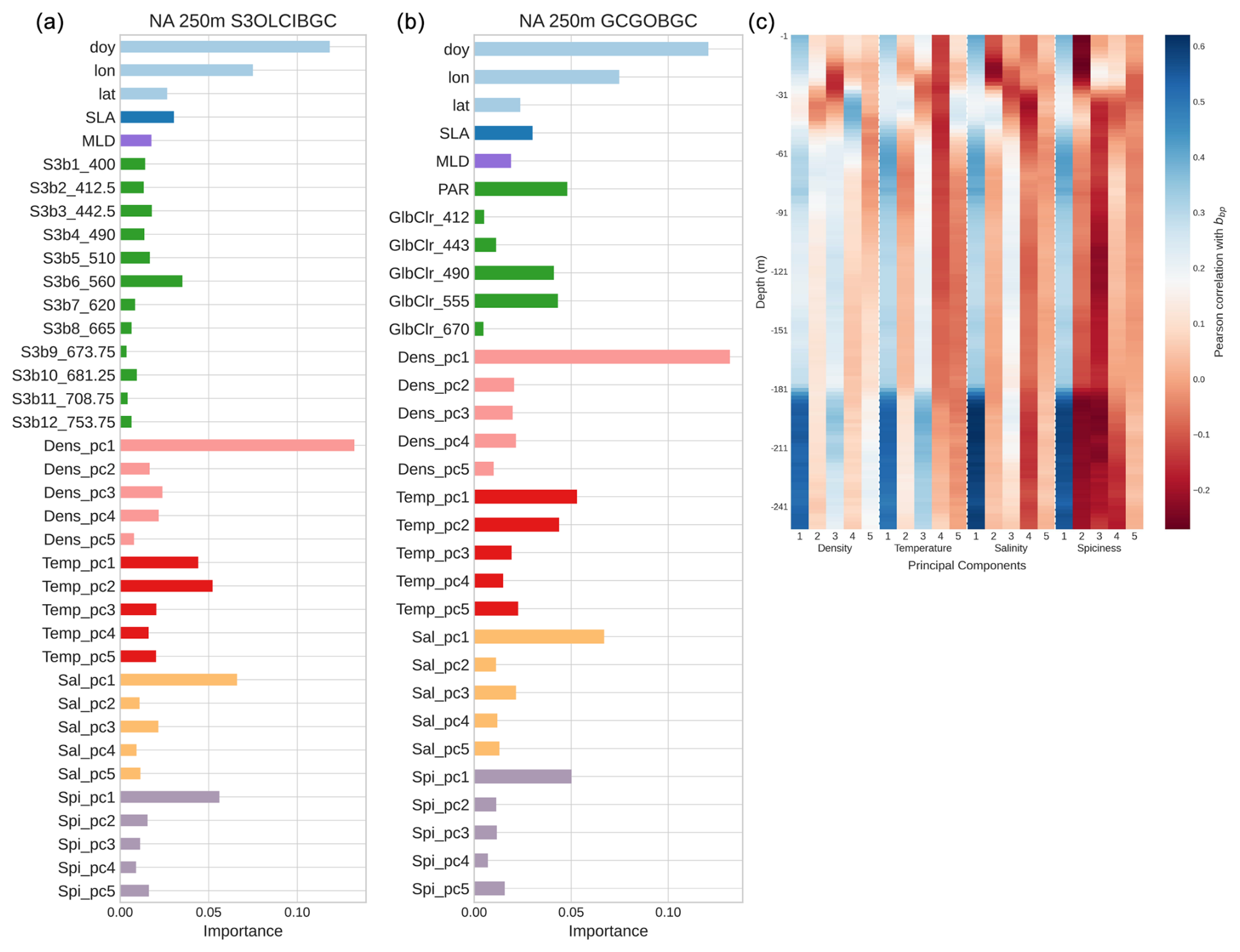
Figure 6 (a, b) Feature importance of the S3OLCIBGC and GCGOBGC models for b_bp estimation down to 250 m in the North Atlantic. (c) Correlation matrix between b_bp and the first five PCs of each BGC-Argo physical variable as a function of depth.

In the STG region, the model performance exceeds that of the North Atlantic, likely due to the more optically homogeneous conditions despite the strongly stratified nature of these oligotrophic waters (Fig. 5c). Similar patterns have been observed in stratified waters, where optical properties like beam attenuation remain relatively homogeneous (Kitchen and Zaneveld, 1990). While the average MLD is around 50 m, no significant increase in error is observed until approximately 120 m. This deeper threshold aligns with the region typically associated with the deep biomass maxima (DBM), which form at the interface between the nutrient-depleted surface layer and the light-limited mesopelagic zone (Cornec et al., 2021). In the STG, this transition zone, often located between 150 and 200 m (Mignot et al., 2014), appears as a boundary where the predictive skill begins to slightly decline – reflected in the gradual increase in the relative error and a subtle shift in the bias profiles. Feature importance for the STG 250 m models is not shown, as it is similar to that obtained in the 50 m models. In both cases, latitude emerges as the most relevant predictor.

3.2 S3OLCI: results of the Sentinel-3 OLCI without BGC-ARGO data

As demonstrated in the previous experiments, satellite-derived features play a significant role in the models when profile depths reach 50 m, thus answering the initial hypothesis of this study. It is clear that sea surface signals help to estimate b_bp at subsurface levels. However, the extent of this contribution across the different depth layers only became evident when comparing models trained with different depth limits. The feature importance of the 50 m depth models shows that, at least in the NA region, the parameters measured by satellite sensors are just as relevant as the inputs from the floats. For this reason, we carried out a last experiment with satellite data (S3OLCI) only to check how the models perform in-depth with the normalized water-leaving reflectance bands. Additionally, we investigated the contribution of satellite-derived IOPs from the C2RCC processor, i.e., adding the absorption and scattering variables as input features (Sentinel-3 OLCI with IOP products – S3IOPs).

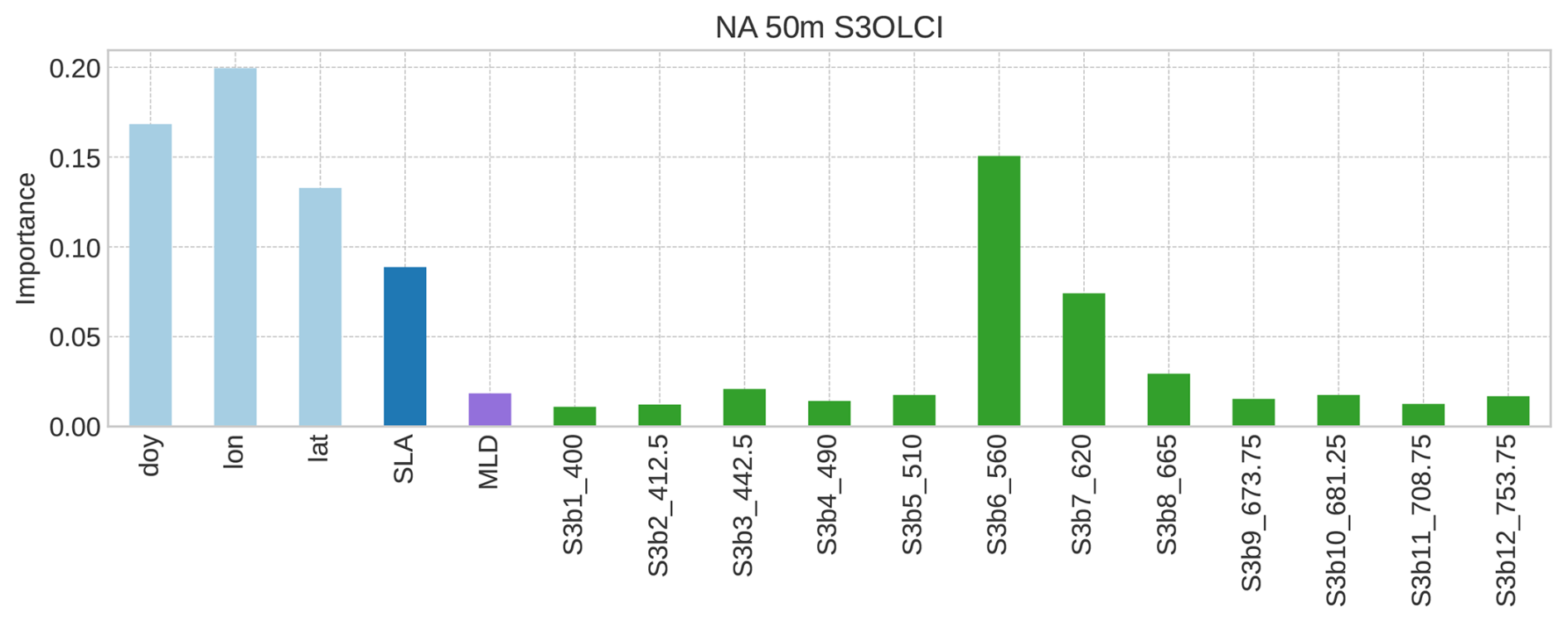
Figure 7 Feature importance of the S3OLCI model for b_bp estimation down to 50 m in the NA area.

In the NA region, the model using only reflectance data (S3OLCI) outperforms the model that includes both reflectance and the absorption and scattering (S3IOPs) (Table 3 and Fig. 8a). While the MLD is still a barrier, the accuracy improves beyond this depth for another approximately 10 m. In the b_bp profiles (Fig. 8b), despite the errors noted in deeper estimations, the model is capable of predicting significant contrast events using only surface data from 36 m onward, except in a specific case characterized by high b_bp values (profile 59). In the feature importance ranking (Fig. 7), the 620 nm band is the most relevant of the spectrum. However, the spatiotemporal features (day of year, longitude, and latitude) seem to have greater weight than the results obtained with the datasets that include BGC-Argo data at the same depth (see Sect. 3.2.1).

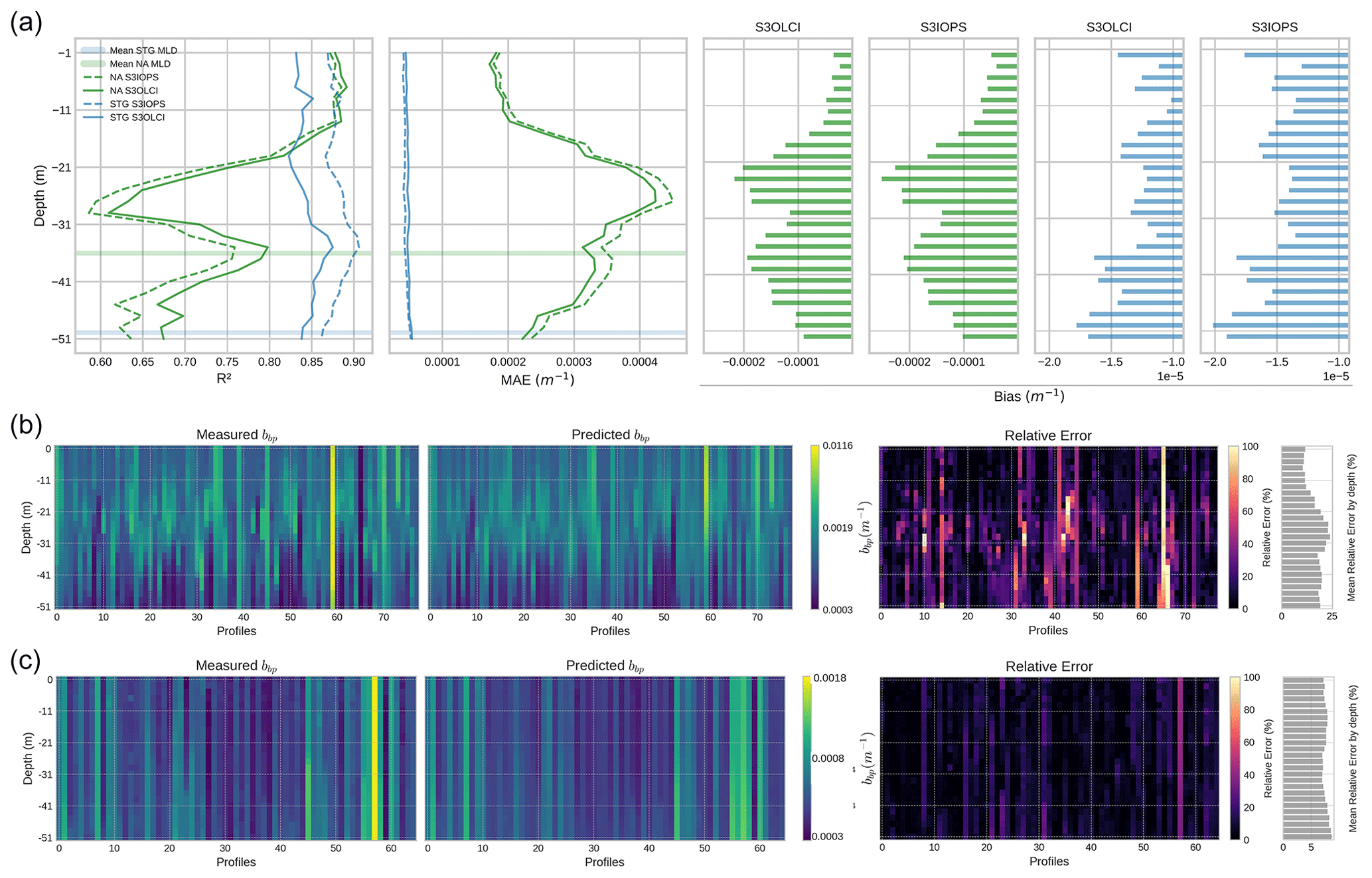
Figure 8 Model performance for estimating shallow water b_bp profiles (0–50 m) with satellite data only. (a) Depth-resolved metrics comparing model predictions using S3OLCI and S3IOPS as inputs: R², MAE, and bias. The shaded horizontal lines indicate the average MLD per region. (b–c) Measured and predicted b_bp profiles in NA (b) and STG (c) using S3OLCI. The rightmost bars show the mean relative error by depth.

In the STG region, the S3IOPs model achieves better results (Table 3). However, it is possible to see how the model is not able to predict some spikes along the water column (Fig. 8c). In the feature importance ranking, latitude remains the most relevant feature. The improved performance of the S3IOPs model, compared to the S3OLCI (reflectance-only) model, could be attributed to the contribution of the marine particle scattering at 443 nm (iop_bpart) provided by the C2RCC processor.

3.3 Validation with independent floats

The previously trained RFR models are applied to predict b_bp values using independent float data that are not included in the training or testing sets. Statistical metrics and the corresponding scatterplots are provided in Table 4 and Fig. 9.

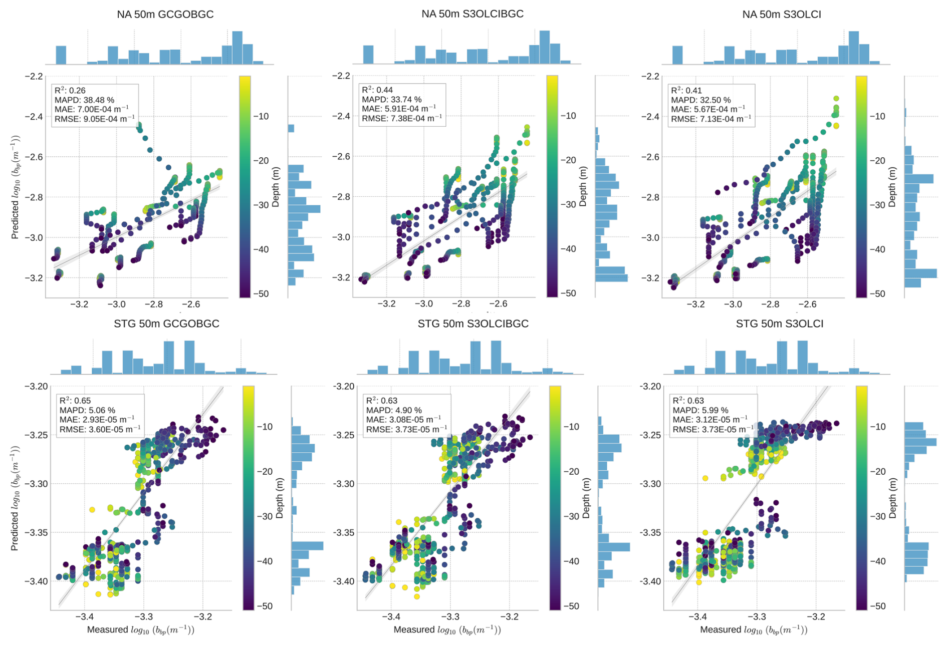
Figure 9 (a) Scatterplots with marginal histograms with the validation of the 50 m model performance on an independent float in the NA region (ID 6902545) and (b) the STG region (ID 3902125). The color scales show the depth of the measurements, and the b_bp values are in log10.

Table 4 Validation results using independent BGC-Argo floats by region at depths of 50 and 250 m. The performance metrics include R², MAPD (%), MAE (m⁻¹), and root mean square error (RMSE; m⁻¹). The models are based on different input datasets: GCGOBGC, S3OLCIBGC, S3IOPs, and Sentinel-3 OLCI reflectance (S3OLCI).

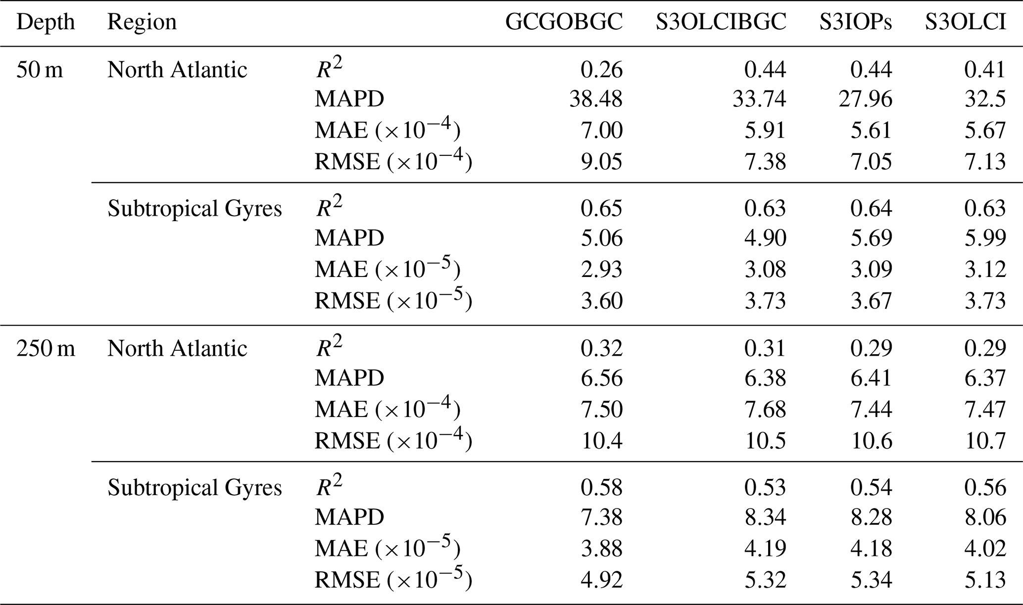
In the NA region, the float identified as WMO 6902545 (see the location in Fig. 1) yields better estimates with the S3OLCI models (R² ranging from 0.41 to 0.44) compared to the reference GCGOBGC model, where the R² value drops to 0.26. This improvement is also visible in the absolute and relative error estimations (MAE and RMSE). Figure 9a reveals the higher b_bp variability in the water depth in the NA region, as indicated by the color scale. There is an overestimation in the surface measurements (less than 30 m) and a slight underestimation at deeper depths. This validation set includes data from several dates in 2017 and 2018, spanning the period from April to August. These temporal variations explain some of the observed drifts in the plots, where different float cycles (water depth profiles) are also evident.

The STG statistics and plots for the float with identifier 3902125 show better correlation coefficients and lower errors compared with the NA. The datasets incorporating S3OLCI data yielded the best results. In Fig. 9b, two clusters of data are visible: one associated with low b_bp values and the other clustering around slightly higher values. The models tend to underestimate the lower b_bp values, while the higher values show a closer fit to the 1 : 1 line. However, in the model that only uses reflectance data (S3OLCI), a clear overestimation of higher values occurs. Unlike in the North Atlantic region, depth separation is not evident here, but the lower values correspond to measurements taken during the winter months in the South Atlantic Gyre, while the higher values were recorded during the summer months in the Southern Hemisphere, where the float was located. These results reinforce the observations made in the previous sections: models provide more accurate b_bp estimations in the STG region than in the NA, confirming the effectiveness of using the S3OLCI bands and derived C2RCC IOPs at shallow water depths.

4 Discussion and conclusion

Previous studies estimating b_bp from satellite-derived remote sensing reflectance (R_rs) have typically employed traditional statistical approaches mostly focused on surface layers. In Bisson et al. (2019), b_bp profiles from floats were processed by averaging b_bp values within the surface mixed layer, followed by a comparison between different sensors and b_bp retrieval inversion products from NASA. In that case study, the OLCI – with data from the reduced-resolution mode at 1.2 km pixel resolution – under-performed compared to MODIS (Moderate Resolution Imaging Spectroradiometer), with 1 km at nadir (r=0.32 to 0.47 and r=0.60 to 0.79, respectively). This difference was attributed to higher coefficients of variation (30 % for the OLCI and 5 % for MODIS) across bands between 412 and 555 nm and an aerosol optical thickness at 865 nm. In the present work, OLCI full-resolution data, with a spatial resolution of 300 m, are used. Additionally, the most relevant wavelength in some of our models (620 nm) was not considered in Bisson et al. (2019).

In the present study, vertical estimates of b_bp are calculated along the water column. We have applied a multi-output random forest model, which shows promising results, especially within the first 50 m in the Subtropical Gyres. However, in dynamic regions such as the North Atlantic, the results are less consistent, suggesting that further research is needed to understand how the complexity of the physical state of the water column modifies the b_bp vertical fluxes. Nevertheless, the focus of our work is on the analysis of the contribution of satellite-derived water-leaving reflectance to b_bp estimation within the first 250 m.

In the deeper layers, where biogeochemical processes like particle sinking, remineralization, and carbon export are more pronounced, the relationship between physical stratification and b_bp seems to become stronger and more linear. In contrast, the correlation between these variables is weaker – though still positive – in the upper layers (0–30 m) and below the mixed layer depth (61–91 m). Density and temperature can offer additional insights into the upper water column, helping to pinpoint processes associated with the depth and intensity of the pycnocline or the MLD. Collectively, these physical features could allow the model to infer the transfer of b_bp from the sunlit surface to the twilight zone by learning from stratification patterns.

Satellite features have indeed proven to be relevant for b_bp estimations, especially in the Subtropical Gyres region, as mentioned. These waters, characterized by high stratification, rely heavily on nutrient injection from deeper zones, as the upper euphotic zone is typically nutrient-limited. In fact, Letelier et al. (2004) and Mignot et al. (2014) describe these gyres as a two-layer system: upper-layer nutrient-limited but not light-limited, with a deeper layer that is light-limited but that has greater nutrient access. These authors also highlight a seasonal distinction, with winter bringing greater water mixing than summer. During winter, the average light intensity for PAR in the mixed layer decreases, while turbulence increases. This seasonal variation may explain the two distinct clusters observed in the validation exercise for the STG region, since two clusters of data are observed, one belonging to the winter of 2017 with slightly higher values and the second coincident with the spring and summer of 2018.

The inclusion of satellite surface data, along with derived parameters such as inherent optical properties (IOPs), in combination with in situ profile data, should be considered for estimating b_bp and, by extension, approximating particulate organic carbon (POC), at least for layers up to 250 m depth. It is important to note that organic carbon fixation primarily occurs in the upper-ocean layers. This organic matter is subsequently transformed through respiration, particle aggregation, zooplankton grazing, feces production, and microbial decomposition (Siegel et al., 2014) before a fraction of it sinks to deeper layers.

The models that relied exclusively on satellite data (S3OLCI and S3IOPs) produced reasonable estimations for the upper layers in both the North Atlantic and Subtropical Gyres regions. This is encouraging, as satellite data, with their synoptic spatial coverage, can efficiently complement Argo float measurements. Satellite observations provide valuable insights into mesoscale ocean processes over various temporal ranges, extending at least the past 3 decades. Since remote sensing products can only reach about 20 % of the euphotic zone, the importance of extending surface observations to deeper layers using autonomous floats or other devices is critical (Claustre et al., 2010).

Future work should be focused on enlarging the database with new BGC-Argo profiles and satellite data, extending the study to new areas of the global ocean. Another detail that could enrich the analysis is the role of the MLD in the different regions in order to further understand the effect that it has on biochemical parameter estimations. Sensors with extended capabilities, like the hyperspectral NASA PACE, might also be a research path to follow, since we have seen that adding new wavelengths had a positive effect on the results of our models compared with sensors with less capabilities. Possible improvements in the detection of CDOM with the UV bands can be an important contribution to better estimating particulate organic material (POM) and, consequently, POC. It has been determined that there is an increase in photoproduction of CO₂ from CDOM (Bélanger et al., 2006) due to the increase in UV radiation and the decrease in sea ice because of the rise in global temperatures. Organic carbon is separated into particulate and dissolved organic carbon (DOC). There is a potential use of CDOM to improve DOC estimations (especially in coastal waters), together with physical variables like sea surface temperature or salinity. If CDOM can really improve DOC estimations and we can do this globally with satellites, a better understanding of the relationship between DOC and POC could also be analyzed temporally and spatially.