Application of the HIDRA2 deep-learning model for sea level forecasting along the Estonian coast of the Baltic Sea

Sea level predictions, typically derived from 3D hydrodynamic models, are computationally intensive and subject to uncertainties stemming from physical representation and inaccuracies in initial or boundary conditions. As a complementary alternative, data-driven machine learning models provide a computationally efficient solution with comparable accuracy. This study employs the deep-learning model HIDRA2 to forecast hourly sea levels at five coastal stations along the Estonian coastline of the Baltic Sea, evaluating its performance across various forecast lead times. Compared to the regional NEMO_BAL and subregional NEMO_EST hydrodynamic models, HIDRA2 frequently outperforms both, particularly in terms of overall forecast skill. While HIDRA2 shows limitations in resolving high-frequency sea level variability above (6 h)⁻¹, it effectively reproduces energy in lower-frequency bands below (18 h)⁻¹. Errors tend to average out over longer time windows encompassing multiple seiche periods, enabling HIDRA2 to surpass the overall performance of the NEMO models. These findings underscore HIDRA2's potential as a robust, efficient, and reliable tool for operational sea level forecasting and coastal management in the eastern Baltic Sea region.

1 Introduction

The importance of sea level variability has grown significantly in the context of climate change as higher global temperatures accelerate its complexity (Bindoff et al., 2007; Cazenave et al., 2014). The increasing frequency and severity of extreme weather events, compounded by rising sea levels due to climate change, present pressing challenges for coastal communities worldwide. Accurate and timely forecasting of sea level is essential for effective disaster preparedness, risk mitigation, and coastal management. However, forecasting sea level variability is inherently complex and requires sophisticated models that account for various drivers and uncertainties. Traditionally, sea level forecasting has been accomplished using hydrodynamic models, but these models are subject to a range of uncertainties induced by errors in atmospheric and open boundary forcing fields, as well as physical flux parameterization (Church et al., 2011; Miles et al., 2014; Khojasteh et al., 2021). Errors in regional sea level prediction can arise from inaccurate initial and boundary conditions, models' approximated descriptions of physical environments (e.g., coupling with waves, atmosphere, ice, and runoff), and the nonlinear nature of planetary dynamics (Carson et al., 2019; Ponte et al., 2019; Hamlington et al., 2020).

Despite these challenges, advancements such as assimilation of observation data in hydrodynamic models have shown promise in improving the accuracy of sea level prediction (Bajo et al., 2019; Barron et al., 2004; Tanajura et al., 2015; Liu and Fu, 2018). However, the computational cost of both ocean modeling and data assimilation adds to the complexity and resource requirements of accurately predicting sea levels (Byrne et al., 2023; Bajo et al., 2023). In this regard, the use of data-driven models as a surrogate system can be a promising addition to classic hydrodynamic models for addressing these challenges (Sonnewald et al., 2021). In recent years, machine learning techniques have demonstrated significant potential in enhancing the accuracy and reliability of predictive models in oceanography (Ahmad, 2019; Lou et al., 2023; Jahanmard et al., 2023). Recent studies have highlighted the effectiveness of deep-learning methods in predicting sea level heights across diverse scenarios and basins (Rus et al., 2023; Balogun and Adebisi, 2021; Rajabi-Kiasari et al., 2023; Bahari et al., 2023). However, these studies imply that, unlike hydrodynamic models, deep-learning models require particular structural design and adjustments depending on various objectives, and the specific characteristics of the study area. Additionally, ensemble-based approaches in deep learning, widely employed in practical applications, distinguish themselves from traditional machine learning methods by generating and integrating multiple hypotheses from training data to improve prediction accuracy. This allows for the incorporation of more advanced and diverse algorithms, making it better suited to tackle specific challenges in operational applications (Zhang et al., 2022; Ganaie et al., 2022).

The Baltic Sea, a large, high-latitude, semi-enclosed, and nearly tideless sea located in northern Europe, is a vital marine region characterized by its unique geographical and ecological features. It comprises several sub-basins and is connected to the Atlantic Ocean through the narrow Danish Straits in the southwest. This study specifically focuses on the eastern Baltic Sea, which spans from approximately 21.5–30.5° E longitude and 56.5–61° N latitude. This region encompasses the northeastern Baltic Proper, the Gulf of Finland, and the Gulf of Riga – areas of strategic importance due to the heavy vessel traffic between their populated shores and islands. Understanding sea level changes in the eastern Baltic Sea is therefore vital. Sea level fluctuations affect navigation routes, harbor operations, and maritime safety, making accurate knowledge of these variations essential for stakeholders to manage risks, optimize vessel operations, and ensure efficient trade flows.

Research on sea level variations in the Baltic Sea has revealed a wide range of patterns and trends influenced by numerous environmental factors that vary both spatially and temporally (Andersson, 2002; Ekman, 2009; Hünicke and Zorita, 2016). Historical tide gauge records, used by Jevrejeva et al. (2003) to reconstruct past sea level changes, demonstrate significant interannual and decadal variability attributed to atmospheric pressure fluctuations and shifting wind patterns. Furthermore, the intricate structure of the Estonian coastline, combined with its numerous small islands, poses additional challenges for projecting the impacts of climate change and sea level rise in this region (Johansson et al., 2004; Kont et al., 2008). Although predictions of sea level height on longer temporal scales, such as monthly or weekly, tend to be more accurate due to the smoothing of short-term fluctuations caused by local wind tilt and storm surges (Samuelsson and Stigebrandt, 1996; Scotto et al., 2009; Elken et al., 2024), short-term sea level changes in the Baltic Sea are heavily influenced by dynamic factors such as wind, precipitation, and the redistribution of water through the Danish Straits (Hünicke et al., 2015). Extreme sea levels on the Baltic coasts, resulting from increasingly frequent storm surges, are influenced by three main factors: the volume of water in the Baltic Sea's basins, which sets the initial sea level; the direction, speed, and duration of tangential wind stresses, whether shoreward or seaward; and the rapid passage of deep low-pressure systems that deform the sea surface, producing seiche-like oscillations that further alter sea levels (Kulikov and Medvedev, 2013; Wolski et al., 2014; Weisse et al., 2021; Wolski and Wiśniewski, 2021; Rutgersson et al., 2022). Seiche oscillations are especially significant in the Baltic Sea due to their prolonged decay over several days. Both the Gulf of Riga and the Gulf of Finland can experience their own seiches with different characteristics (e.g., the 5 h seiche period of the Gulf of Riga, which differs from the recognized seiche period in the Gulf of Finland). These seiches may interact with those from neighboring basins (e.g., the approximately 27 h seiche period of the entire Baltic Sea), leading to complex phase relationships and further complicating sea level predictions (Metzner et al., 2000; Suursaar et al., 2002; Jönsson et al., 2008). This intricate interplay of atmospheric, oceanic, and coastal dynamics makes the prediction of sea level in the Baltic Sea a challenging task.

In response to the increasing demand for accurate and efficient forecasting methods in coastal regions, this study explores the potential of a deep-learning ensemble model. By utilizing deep neural networks, we aim to improve sea level prediction accuracy in the eastern Baltic Sea by applying our approach to a selection of sample stations. The primary focus of this study is to evaluate the effectiveness of a deep-learning ensemble model HIDRA2 (Rus et al., 2023) for sea level forecasting in the study area in multiple lead time windows. A secondary objective is to compare its performance with that of regional and subregional hydrodynamic models currently used for operational purposes in the study area.

2 Data and methods

2.1 Tide gauge data

The hourly sea surface height (SSH) time series were extracted and evaluated as measures of sea level using the available data from five observation stations: Narva-Jõesuu, Pritia, Haapsalu, Pärnu, and Roomassaare (Fig. 1). These stations are situated along the Estonian coast, in the Gulf of Finland and the Gulf of Riga. The datasets were provided by the Estonian Environmental Agency (https://www.ilmateenistus.ee/, last access: 4 April 2024) and span the period between 15 June 2010 and 30 April 2024.

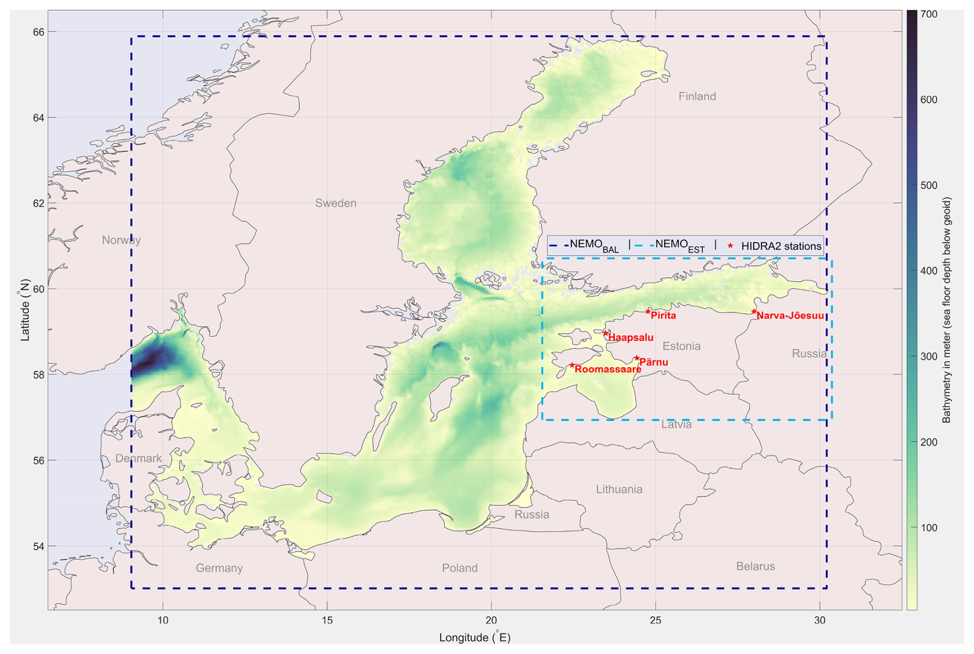
Figure 1 Study area: the domain of each model is illustrated, with red stars indicating the locations of the stations where HIDRA2 has been applied.

2.2 HIDRA2: a deep-learning ensemble sea level forecasting model

HIDRA2 is a state-of-the-art deep-learning model for predicting SSH at specific geographic locations, presented in depth in Rus et al. (2023). The model utilizes historical and predicted atmospheric data, tidal information, and observed SSH measurements to generate precise hourly SSH predictions for a 72 h window. Unlike models that forecast the residual SSH, i.e., the difference between SSH and tide, HIDRA2 predicts the full SSH. The HIDRA2 architecture, illustrated in Fig. 2, incorporates specialized encoders for processing both atmospheric data and sea level inputs. The atmospheric encoder processes wind and pressure sequences, subsequently merging them into a unified feature representation. The SSH encoder processes historical SSH data. In the fusion-regression block, all extracted features with the preceding 72 h raw SSH data are fused and regressed into final SSH forecasts. These encoders consist of a series of convolution layers, activation functions, dropout layers, and skip connections, forming a robust and deep neural network. Details of the encoding architecture are presented in Rus et al. (2023). The specific difference in this study for the Baltic Sea application is that, unlike in Rus et al. (2023), HIDRA2 was trained on the full SSH data rather than on separate tidal and SSH signals. This decision was made because tides in the Baltic are very weak, and the explicit inclusion of tides as a separate input signal did not improve forecasting performance. Consequently, we removed the tidal encoder block and fused only the atmospheric and SSH features, augmented by the raw SSH measurements, to produce the final set of 72 h SSH predictions.

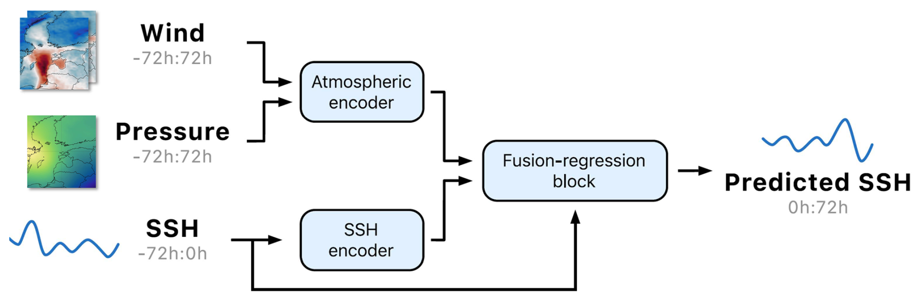
Figure 2 HIDRA2 architecture. The structure of the building blocks is inherited from HIDRA2 and explained in detail in Rus et al. (2023).

For the training of HIDRA2, we utilized atmospheric data fields from the European Centre for Medium-Range Weather Forecasts (ECMWF) Ensemble Prediction System (Leutbecher and Palmer, 2007). For all locations, we used 10 m winds and mean sea level air pressure from a single atmospheric ensemble member, covering a longitudinal range from 16.25 to 28.5° E and a latitudinal range from 54.25 to 64° N. This selection was guided by iterative testing aimed at minimizing forecast errors. The original meteorological data, with a domain size of 40×50, were subsampled to a 9×12 grid using bilinear interpolation to match HIDRA2's required input size. This transformation reduced dimensionality while preserving key spatial patterns, facilitating more efficient model training. We also conducted experiments using the full-resolution atmospheric fields. These trials involved necessary adjustments and fine-tuning of the model. However, we found that the resulting performance metrics were comparable to those achieved with the subsampled data, showing no significant improvement despite the increased computational demand. Given the similar performance and the considerable advantage in computational efficiency, we retained the subsampled approach for the results presented. The training data for SSH at the coastal stations were obtained from the Estonian Environmental Agency as mentioned in Sect. 2.1. However, the SSH data used for training consisted of hourly observations from 2010 to 2019 at all locations, while the period from April 2023 to April 2024 was utilized for testing the model and performing the analyses presented in this study. Following the methodology outlined by Rus et al. (2023), we trained a separate HIDRA2 model for each of the five geographic locations depicted in Fig. 1.

2.3 NEMO_BAL: a forecast product based on a regional hydrodynamic modeling

We extracted the Baltic Sea Physics Analysis and Forecast datasets (BALTICSEA_ANALYSIS_FORECAST_PHY_003_006, 2024) from the Copernicus Marine Service for each station in the study area over the study period. This forecast product is based on the NEMO 4.0 ocean engine, specifically configured for the North Sea and Baltic Sea as Nemo-Nordic 2.0 (Madec et al., 2017; Kärnä et al., 2021), and has been implemented and validated by the Baltic Monitoring and Forecasting Centre (BALMFC) to address the needs of the Baltic Sea region. For brevity, we refer to it as NEMO_BAL in this study. The product offers a spatial resolution of 1 nautical mile (nmi) and is updated twice daily, providing new 6 d forecasts. Consequently, the dataset records available from Copernicus include only 12 h forecasts. The detailed validation report is given in Jandt-Scheelke et al. (2023).

2.4 NEMO_EST: a subregional hydrodynamic forecasting model

NEMO-EST05 is the Estonian adaptation of the Baltic Sea regional configuration Nemo-Nordic 2.0 with enhanced horizontal and vertical resolution, tailored for national operational purposes (hereafter referred to as NEMO_EST). Detailed specifications of this model are provided in Maljutenko et al. (2022), and an example of its utilization is presented in Pärt et al. (2023). NEMO_EST uses the same NEMO 4.0 ocean engine with a horizontal resolution of 0.5 nmi spanning from 21.5 to 30.5° E and from 56.5 to 60.5° N. The meteorological forcing for the model system is obtained from the ECMWF 24 h integrated forecasting system (Owens and Hewson, 2018). Boundary conditions for salinity, temperature, and sea levels are derived from the same NEMO_BAL, following the methodology outlined by Elken et al. (2021). Model initialization in the October 2022 is from the NEMO_BAL. It can be inferred that NEMO_EST serves as a downscaled version of NEMO_BAL. Therefore, using both models in the present study also provides implicit insights into how the spatial resolution of hydrodynamic models, as well as their domain extent, affects SSH forecasting.

2.5 Forecasting and evaluation framework

HIDRA2 and NEMO_EST provide SSH forecasts for the next 72 h, segmented into three 24 h intervals: 0 to 24 h (24), 24 to 48 h (48), and 48 to 72 h (72), with daily updates. This segmentation allows for the evaluation of model performance at different lead times up to 72 h. Regardless of the training time window used for the deep-learning model, the testing period of all models in the present study spans 1 year, from 1 April 2023 to 31 March 2024 (in total, 8784 h time instances). This period aligns with the initiation of archiving 72 h SSH fields in NEMO_EST from its daily forecast cycles. For comparison, NEMO_BAL was also considered as the publicly available SSH forecast for the study area. To ensure a fair comparison and address potential bias from the reference sea level in the hydrodynamic models (NEMO_BAL and NEMO_EST), the outputs were adjusted by removing their mean value over the study period and then adding the mean observed SSH at each station. This adjustment to the datums of the local observation system ensures that the outputs of the hydrodynamic models are comparable to the observed values, whereas HIDRA2, as a data-driven model, is not subject to this type of reference sea level bias. Additionally, HIDRA2, as an ensemble forecasting system, produces 50 distinct forecast ensembles at each time point. In the analysis, unless specifically examining individual ensembles, the HIDRA2 forecasts are represented by the average of all 50 ensembles for each time instance and station. Using the mean of all ensembles as the final forecast is appropriate because the ensembles represent probabilities without any inherent priority in real-world occurrences.

Furthermore, the performance of the forecasts is also separately evaluated during extreme negative and positive observed SSH events. Extreme negative SSH values are defined as those falling below the 5th percentile of observed SSH at each station during the study period, while extreme positive values are those exceeding the 95th percentile (Cannaby et al., 2016; Mentaschi et al., 2023).

2.6 Validation metrics

The validations and comparisons in the present study include the Pearson correlation coefficient (correlation) and the root mean square deviation (RMSD). Each is defined as follows.

RMSD is given by Eq. (1):

$$\begin{array}{}\text{(1)}& {\displaystyle }{\displaystyle }\text{RMSD}={\left({\displaystyle \frac{\mathrm{1}}{n}}\sum _{i=\mathrm{1}}^n(o_i-m_i{)}^{\mathrm{2}}\right)}^{\mathrm{1}/\mathrm{2}},\end{array}$$

where n represents the total number of observations, and o_i and m_i are the observed and modeled sea level values, respectively.

Correlation is defined by Eq. (2):

$$\begin{array}{}\text{(2)}& {\displaystyle }{\displaystyle }\text{correlation}={\displaystyle \frac{\mathrm{1}}{{\mathit{\sigma }}_{\mathrm{m}}{\mathit{\sigma }}_{\mathrm{o}}}}\sum _{i=\mathrm{1}}^n(m_i-\stackrel{\mathrm{‾}}{m})(o_i-\stackrel{\mathrm{‾}}{o}),\end{array}$$

where $\stackrel{\mathrm{‾}}{m}$ and $\stackrel{\mathrm{‾}}{o}$ are the mean values of the modeled and observed datasets, respectively.

The standard deviations of the modeled and observed datasets, σ_m and σ_o, are calculated as shown in Eq. (3):

$$\begin{array}{}\text{(3)}& {\displaystyle }{\displaystyle }{\mathit{\sigma }}_{\mathrm{m}}={\left(\sum _{i=\mathrm{1}}^n(m_i-\stackrel{\mathrm{‾}}{m}{)}^{\mathrm{2}}\right)}^{\mathrm{1}/\mathrm{2}},{\mathit{\sigma }}_{\mathrm{o}}={\left(\sum _{j=\mathrm{1}}^n(o_j-\stackrel{\mathrm{‾}}{o}{)}^{\mathrm{2}}\right)}^{\mathrm{1}/\mathrm{2}}.\end{array}$$

The validation metrics for each station are calculated using referenced to the SSH observation data from April 2023 to April 2024.

3 Results

3.1 Comparison of models' overall performance

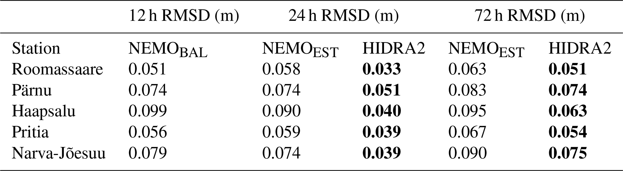
Table 1 presents the RMSD values for the forecasts across all tide gauge stations relevant to availability of the model outputs in the present study. At 24 h lead time, the HIDRA2 ensemble mean consistently achieves the lowest RMSD at each station, outperforming even NEMO_BAL, which inherently includes 12 h lead-time forecasting. HIDRA2 with a 72 h lead time also demonstrates performance comparable to NEMO_BAL at Roomassaare and Pärnu. Remarkably, HIDRA2 exhibits substantially lower RMSD at other stations, even with extended forecast lead times.

Table 1 RMSD metrics of the three forecast models for the April 2023 to April 2024 period. Results are separated by the forecast lead times (12, 24, and 72 h). Lowest RMSDs are in bold.

Several studies such as Campos-Caba et al. (2024) and Mentaschi et al. (2013) have highlighted limitations in using the RMSD as a standalone performance metric, particularly due to the double-penalty effect. This occurs when temporal mismatches between modeled and observed seiches lead to models being penalized twice: once for predicting a peak that did not occur and again for failing to predict one that did. As a result, RMSD may not fully capture the quality of model predictions. To address this, RMSD should be interpreted alongside complementary performance metrics. For instance, Campos-Caba et al. (2024) propose evaluating the mean absolute deviation, adjusted across percentiles by the corresponding mean absolute deviation of each percentile from the 0th to the 100th percentile in 1 % steps.

We therefore recommend that Table 1 and the RMSD values be considered in conjunction with the model error across all sea level bins (Fig. 3) and further contextualized through spectral analysis of model and observed time series.

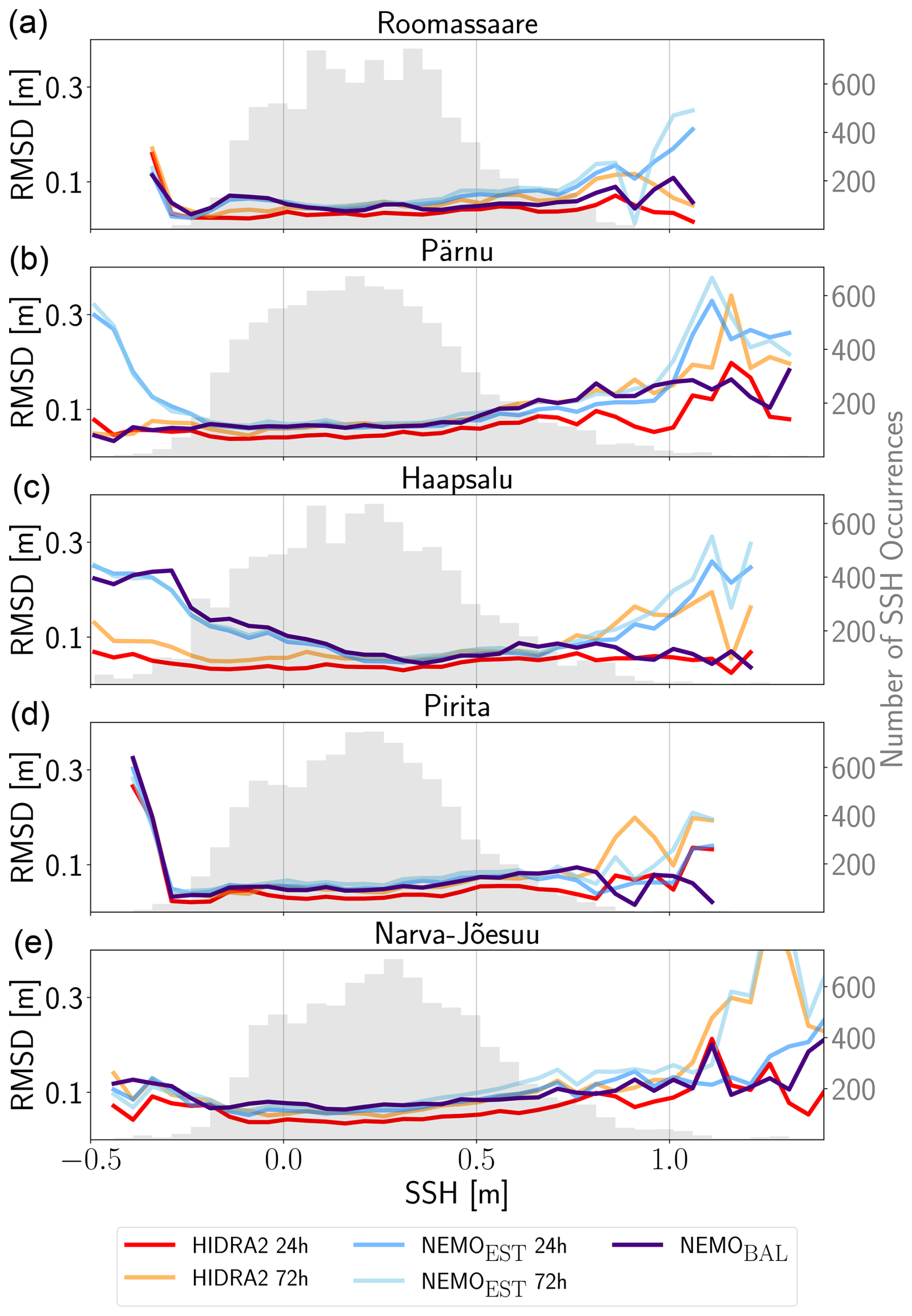
Figure 3 RMSD of all forecast models (colored lines; see legend at the bottom) at different sea level values. Grey histogram in the back (right axis) shows the distribution of occurrences of a given sea level bin.

Figure 3 illustrates the forecast RMSD by sea level bin (0.05 m) for all models at different lead times. HIDRA2 with a 24 h lead time generally outperformed the other models, achieving the lowest RMSD across most of the sea level distribution, i.e., at all sea level percentile bins p. However, in the tails of the distribution (SSH>1.00 m or $\text{SSH}<-$0.40 m), RMSDs increased for all models. At extreme sea levels, HIDRA2 and NEMO_BAL demonstrated similarly robust performance, albeit with differences depending on lead time. HIDRA2 showed solid performance at the 24 h lead time but struggled in the distribution tails at the 72 h lead time.

Figure 3 highlights that HIDRA2's advantage over NEMO_BAL primarily stems from its superior performance in the bulk of the distribution and at extreme low SSH values. This distinction is particularly evident at the Haapsalu station.

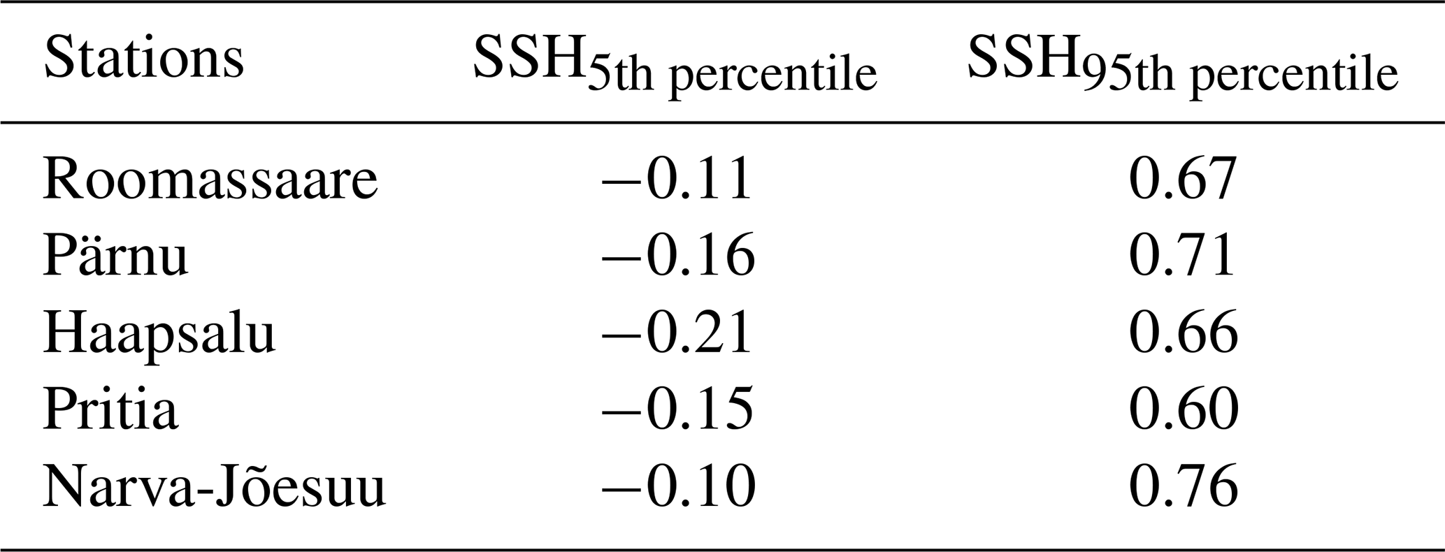
Additionally, the accuracy of each model, integrated across all study stations, is compared using Taylor diagrams (Taylor, 2001) in Fig. 4a. The 5th and 95th percentile thresholds for each station are provided in Table 2. HIDRA2 consistently outperformed both hydrodynamic models, showing the lowest RMSD and highest correlation coefficients across most observed SSH ranges. Although HIDRA2's accuracy declines for extreme SSH values, particularly at extended lead times, it still surpasses both regional and subregional hydrodynamic models, except at 72 h lead time. Among the hydrodynamic models, the regional model NEMO_BAL performs best during extreme SSH events, while the subregional model NEMO_EST performs better under non-extreme high SSH conditions but struggles to accurately predict extreme SSH values.

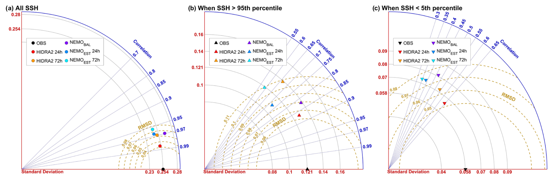
Figure 4 Taylor diagrams comparing forecasts: (a) all hourly time instances, (b) positive extreme SSH, and (c) negative extreme SSH.

Table 2 Thresholds for SSH used to identify extreme positive and negative storm surges at each station.

We perform an independent analysis of the predictive accuracy across the 50 members of the HIDRA2 ensemble, evaluating each member's forecasts of SSH values. As expected, increasing the lead time of forecasts results in reduced accuracy of each predicted ensemble member. Both the correlation coefficient and RMSD vary across different lead times, and the spread of ensemble predicted values increases with longer lead times. This spread is especially pronounced during extreme observed SSH values. For negative extreme SSH events, correlation is lower with a lower RMSD, while for positive extreme SSH events, correlation is higher but with a higher RMSD (Fig. 5).

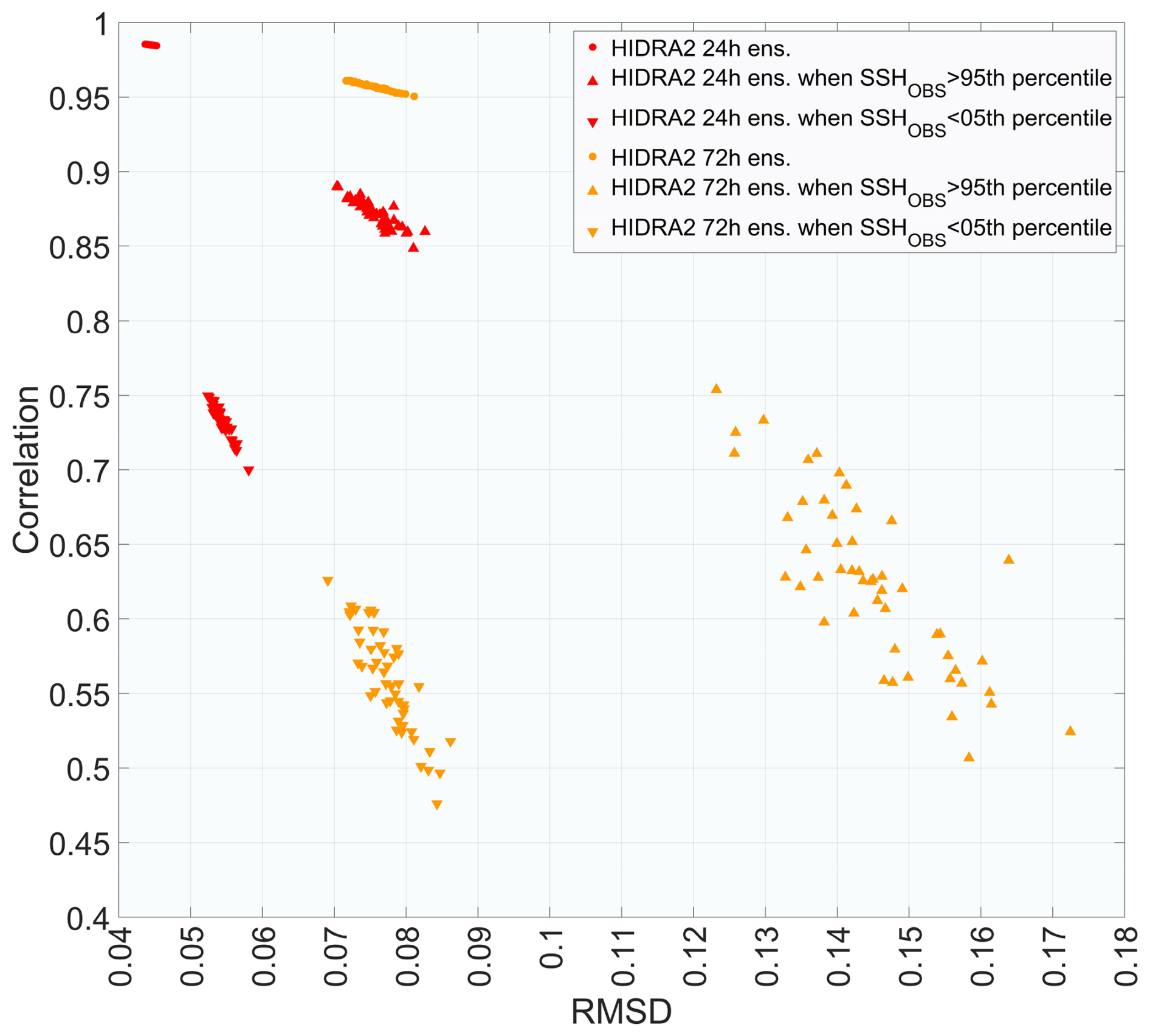
Figure 5 Performance of individual HIDRA2 ensemble members at 24 and 72 h lead times and a further assessment under the conditions of the positive and negative extreme observed SSH.

3.2 Specific challenges in model performance

Overall, HIDRA2 forecasts with a 24 h lead time consistently outperformed throughout the study period at all stations, as detailed in Table 1 (an overview of the reliable forecast capabilities of HIDRA2 is also provided in the Supplement). However, a closer examination, as shown in Fig. 6, reveals that HIDRA2 predictions are overly smoothed, lacking the ability to fully capture high-frequency variability (with periods below 6 h). In contrast, NEMO_BAL demonstrates better performance in this energy band. Figure 6 highlights model forecasts with a 24 h lead time during October 2023, a period marked by a series of extreme sea level events.

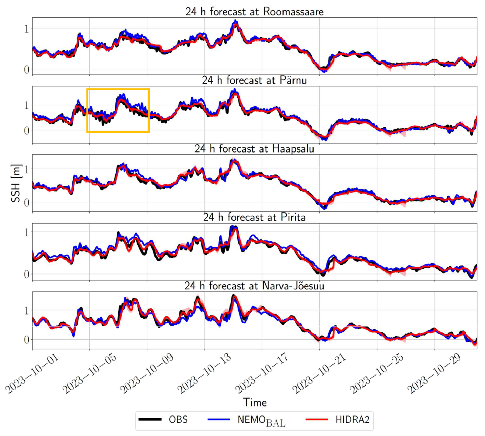
Figure 6 Observed SSH (black line) vs. NEMO_BAL (blue line) and HIDRA2 ensemble mean (red line) forecasts with a 24 h lead time at various stations during October 2023.

A visual comparison of model predictions in Fig. 6 between 5 and 9 October 2023 is highly indicative. (To further aid recognition, this specific time window is highlighted by an orange box in Fig. 6.) Sea levels in Pärnu indicate the presence of the fundamental seiche with a period around 5 h. NEMO_BAL reproduces this excitation very clearly, while it is practically completely absent from the HIDRA2 forecast. A similar scenario occurs on 13 October – NEMO_BAL exhibits high-frequency variability, whereas the HIDRA2 ensemble mean is completely smooth. This smoothing effect could potentially result from averaging over the ensemble members, where oscillations present in individual members cancel each other out. This is however not the case. None of the ensemble members exhibit enough excitations in the Pärnu seiche energy band (not shown).

The limitations of HIDRA2 during seiche excitations can be evaluated by applying a band-pass filter to the sea level signal in the Pärnu seiche energy band for the period of excited seiches between 5 and 9 October 2023. We use a sixth-order Butterworth filter with a sample rate of 1 h and low and high cutoff frequencies of (3 h)⁻¹ and (8 h)⁻¹, respectively (Fig. 7). The filtered observations in Fig. 7 clearly show the excitation of the seiches starting on 3 October, which is also captured by NEMO_BAL. In contrast, the HIDRA2 ensemble mean is overly smooth, rendering it less capable of reproducing sea level variability within the seiche frequency band. However, it adheres more closely to the overall observations than NEMO_BAL. HIDRA2's limited accuracy during seiche excitations leads to deviations from instantaneous sea level values, increasing the short-term errors. However, over periods of several days, HIDRA2 exhibits minimal bias. This indicates that while individual hourly predictions may show higher error, HIDRA2's forecasts do not consistently over- or underestimate SSH over longer time spans, resulting in minimal systematic bias.

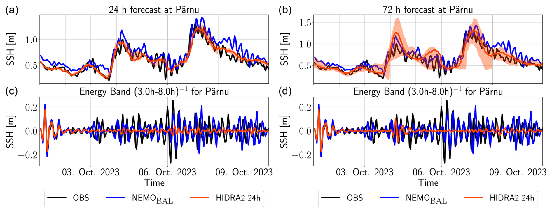
Figure 7 (a, b) Sea levels in Pärnu during the seiche between 5–9 October 2023 for 24 h (a, c) and 72 h (b, d) lead times. Orange area denotes the limits of the HIDRA2 ensemble envelope. (c, d) Bandpass-filtered sea levels in the frequency band (3 h)⁻¹–(8 h)⁻¹ during the same period and for the same lead times. Note the different vertical scales in both plots.

This experiment also demonstrates the value of the ensemble prediction. While separate members of the HIDRA2 ensemble (and consequently their ensemble mean as well) are not capable of capturing the high-frequency variability of the seiche (not shown), this limitation is partly compensated by the ensemble spread, which to some extent envelops the actual amplitude of the seiches. Therefore, the sea levels during the seiche will often still be within the ensemble envelope, although the seiche itself is poorly reproduced in each individual ensemble member. This ensemble approach in HIDRA2 is especially useful for addressing the challenges of triggering events and managing uncertainty in sea level forecasts. Triggering events often involve abrupt and transient atmospheric or oceanic changes, like storms or pressure systems, which lead to rapid sea level shifts. While HIDRA2's ensemble mean may not directly capture these fluctuations, the ensemble spread creates a “buffer” around the observed values. This means that during trigger events, even if individual ensemble members miss exact timings or magnitudes, the ensemble as a whole may still envelop the observed extremes, providing a probabilistic signal of potential risks.

To quantify NEMO_BAL, as well as HIDRA2 behavior in different spectral bands, we computed power spectral densities (PSDs) for observations and model forecasts for each of the stations, as shown in Fig. 8. The PSD was calculated by normalizing the squared magnitude of the fast Fourier transform coefficients at each frequency, followed by an inversion of frequencies to periods. This allowed us to identify dominant seiche periods and the (ir)relevance of tidal forcing (peaks around 12 and 24 h). In Pärnu, for example, the fundamental seiche peak close to 6 h period is quite prominent, while the semi-diurnal 12 h peak does not stand out in its energy band, indicating that semi-diurnal tides are not driving the dynamics at this station. At other stations, for example, semi-diurnal tides are a bit more pronounced.

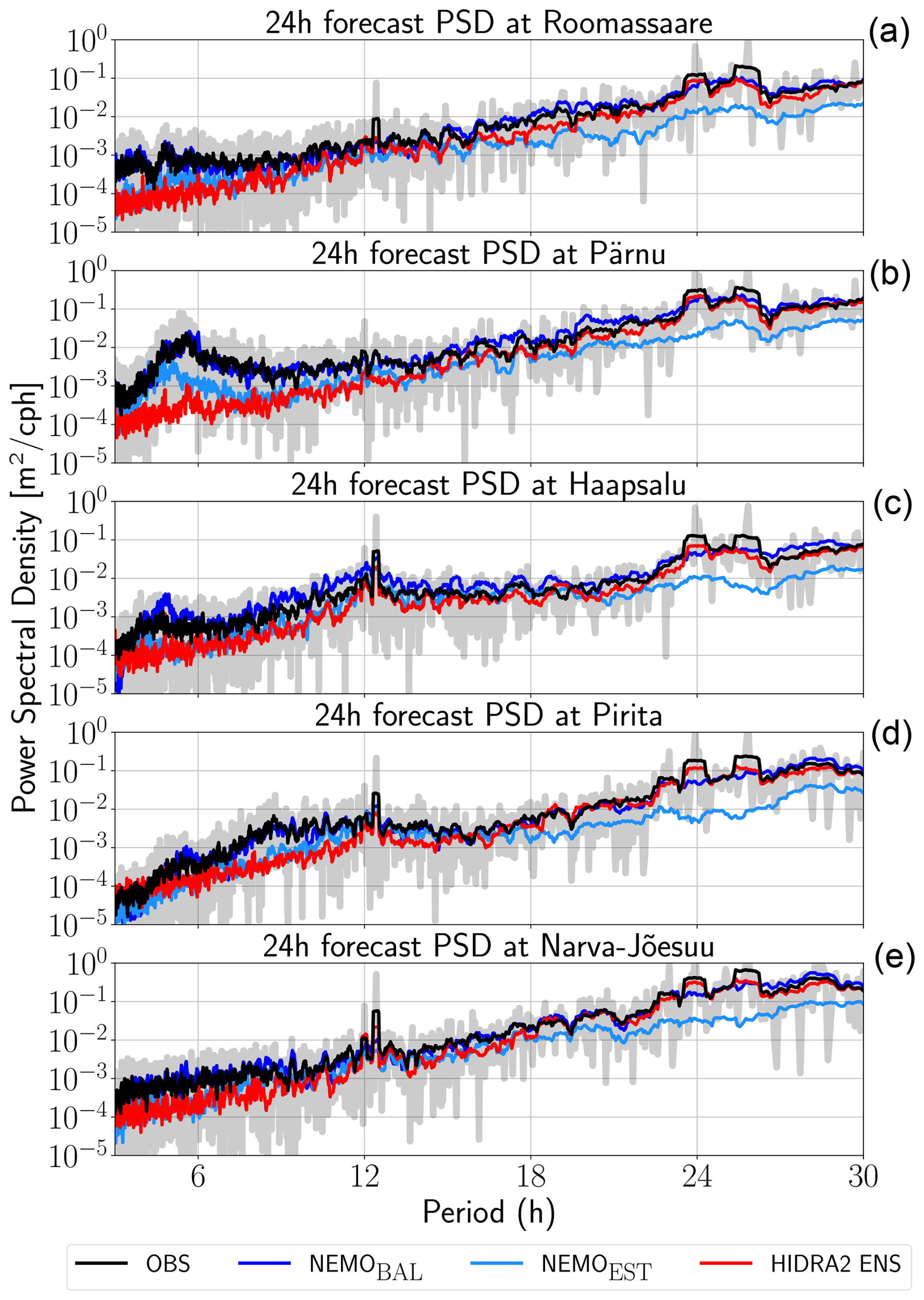
Figure 8 Power spectral densities [m² cph⁻¹] of sea levels from different sources (colored lines; see legend at the bottom) at each station (rows). Grey lines in the back denote raw spectra, while black lines denote their 6 h moving average; cph indicates cycles per hour.

The spectra reveal that HIDRA2 faces challenges in fully capturing seiche dynamics and tends to underestimate energy density in the subinertial energy band (at the latitude of Pärnu, this corresponds to periods below 13 h or rather frequencies above (13 h)⁻¹) – in this band NEMO_BAL accurately reproduces the observed amount of energy. HIDRA2 spectra are however the closest to observations spectra in the band with periods above 18 h. Especially at diurnal tide band HIDRA2 shows slightly better performance than NEMO_BAL, while both HIDRA2 and NEMO_BAL outperform NEMO_EST. This corresponds to the solid overall performance of HIDRA2 and its poor reproduction of high-frequency variability. NEMO_EST on the other hand lacks almost an order of magnitude of energy in the energy band with periods above 18 h but indicates a decent reproduction of the Pärnu seiche.

4 Discussion

Validation metrics, such as RMSD and correlation coefficient, presented in this study underscore HIDRA2's competitive performance compared to other sea level forecasting methods, as demonstrated in other studies (e.g., Ishida et al., 2020; Shahabi and Tahvildari, 2024; Dong et al., 2024). Despite the influence of various regional factors on short-term SSH forecasts, the primary distinction between HIDRA2 and methods used in previous studies is the utilization of a deep-learning “ensemble” approach. Thus, the effectiveness of HIDRA2 in this case study underscores the importance of incorporating diverse ensembles to account for varying short-term atmospheric conditions and climate scenarios (Gröger et al., 2019; Hieronymus and Hieronymus, 2023). For operational applications, particularly in decision-making and initiating specific response phases, HIDRA2 can be more effective when the triggering limits are set to the maximum and minimum ensemble values, as these represent the most probable scenarios. Although the probability of reaching the maximum or minimum ensemble values in typical cases is around 2 % – given the 50 ensembles used in this study – the ensemble spread, which almost always encompasses the absolute SSH values, suggests that HIDRA2 is a more reliable tool for operational forecasting and triggering. This reliability is especially notable when compared to other forecasting systems that do not provide ensemble predictions. Future studies could further explore optimizing this ensemble range. In the present study, it has been shown that the spread of ensemble-predicted values increases with longer lead times, with this spread becoming particularly pronounced during extreme observed SSH values. When considering a separate evaluation of negative and positive extreme SSH events, the results show that for negative extreme SSH events, the correlation is lower with a narrower RMSD, while for positive extremes, the correlation is higher but accompanied by a wider RMSD. Here, the significance of comparing RMSDs may be less relevant, as higher RMSD values can be acceptable when target values are higher. But, in general, the lower correlation during negative SSH extremes suggests that while the model captures some general trends or patterns, it does not align well with the exact fluctuations or magnitudes of observed values. From a data-driven modeling perspective, this may be explained by data imbalance: negative extreme events are rarer than positive extremes in the study area (Conte and Lionello, 2013; Jensen et al., 2022), providing HIDRA2 with fewer examples of negative events during training. Consequently, HIDRA2 may perform better for positive extreme events, having learned from their relatively higher frequency. This observation demonstrates the model's enhanced capability to capture more common extreme event types. This stems from HIDRA2's data-driven foundation, which allows it to effectively learn patterns from densely populated regions of the training distribution. In contrast, hydrodynamic models, while grounded in first-principles physics, are generally less responsive to data frequency and often lack flexibility in probabilistic forecasting. To further improve HIDRA2's performance across the full range of sea level conditions – particularly in data-sparse regimes – future developments could explore the integration of physics-informed neural networks (Raissi et al., 2019; Zhu et al., 2025). By incorporating physical constraints, such as conservation laws or shallow water dynamics, into the learning process, such approaches can mitigate the effects of limited data availability while guiding the model toward physically consistent behavior, even under rare or extreme scenarios. Looking ahead, combining physics-informed strategies with ensemble-based deep learning may provide a more robust and generalizable framework for sea level forecasting, supporting both routine operations and high-impact coastal applications.

5 Conclusions

This study evaluates an implementation of HIDRA2, a deep-learning sea level model, alongside two numerical models: NEMO_EST, a subregional hydrodynamic model with a spatial resolution of 0.5 nmi, and NEMO_BAL, a regional hydrodynamic model with a spatial resolution of 1 nmi and 12 h lead time. In summary, based on the averaged correlation coefficient and RMSD across the study period between modeled and observed SSH, the results indicate that HIDRA2 generally outperforms the hydrodynamic models.

While accuracy decreases in predicting extreme sea level events, the observed values generally fall within the predicted ensemble spread of HIDRA2, highlighting its overall reliability. However, some open issues remain. HIDRA2 did not perfectly reproduce seiches in Pärnu Bay and in general lacks energy in the subinertial band with periods below 13 h. Reproduction of sea level dynamics in this band is something that will have to be addressed in further work. This can be partly offset by an ensemble spread, but the spread with 24 h lead time is underestimated, while the spread for 72 h seems overestimated, as can be seen from Fig. 7.

These issues might be addressed by further implementations of a very recent version of HIDRA (Rus et al., 2025), which is capable of performing multipoint predictions. Preliminary investigations (not shown) however indicate that high-frequency sea level variability is a very difficult task for classical models and for deep networks. As far as deep networks are concerned, it is currently unclear whether poor reproduction of this spectral band is an issue of architecture or of insufficient training data. In any case this task should have a high priority of research due to its ever-growing relevance for business and safety under most climate change sea level rise scenarios.