the Creative Commons Attribution 4.0 License.
the Creative Commons Attribution 4.0 License.
 | 14 Jul 2025
Constraining local ocean dynamic sea-level projections using observations
Iris Keizer
Sybren Drijfhout
The redistribution of ocean water volume under ocean–atmosphere dynamical processes results in sea-level changes. This process, called ocean dynamic sea level (ODSL) change, is expected to be one of the main contributors to sea-level rise along the western European coast in the coming decades. State-of-the-art climate model ensembles are used to make 21st century projections of this process, but there is a large model spread. Here, we use the Netherlands as a case study and show that the ODSL rate of change for the period 1993–2021 correlates significantly with the ODSL anomaly at the end of the century and can therefore be used to constrain projections. Given the difficulty of estimating ODSL changes from observations on the continental shelf, we use three different methods providing seven observational estimates. Despite the broad range of observational estimates, we find that 4 to 16 CMIP6 models have rates above the observational range and 0 to 1 below. We compare four model selection methods which differ in the way the uncertainty in the rate estimation is considered. We find that for stricter selection methods the rate of ODSL is closer to the observational range, and the uncertainty in future change is reduced. The influence of model selection is largest for the low emission scenario SSP1-2.6. We discuss the advantages and disadvantages of those selection methods and their suitability for different users.
- Article
(5115 KB) - Full-text XML
- BibTeX
- EndNote


Understanding local sea-level rise and providing reliable sea-level projections is an important duty of the scientific community to help society face this challenge (Hinkel et al., 2019; Le Cozannet et al., 2017). Currently, sea-level projections use contributor-based and process-based approaches (Fox-Kemper et al., 2021). Contributor-based means that the projections are the sum of each individual contributor to sea-level rise, and process-based means that when possible the contributors are projected using models of the detailed physical processes (Church et al., 2013; Le Bars, 2018). The contributors considered in projections are glaciers, ice sheets, land water storage, glacial isostatic adjustment from the last glacial maximum, global steric sea level, and ocean dynamic sea level (ODSL). ODSL is defined as “the local height of the sea surface above the geoid with the inverse barometer correction applied” (Gregory et al., 2019). Changes in ODSL are due to changes in winds and ocean currents as well as changes in atmosphere–ocean heat and freshwater fluxes. It is related to both steric and manometric sea-level changes. The contribution of ODSL to local sea-level rise is modelled directly by coupled atmosphere–ocean general circulation models (AOGCMs; Gregory et al., 2019). Therefore, AOGCMs from the Coupled Model Intercomparison Project 5 and 6 (CMIP5 and CMIP6) were the basis for ODSL projections from the Intergovernmental Panel on Climate Change Assessment Report 5 (AR5; Church et al., 2013) and 6 (AR6; Fox-Kemper et al., 2021).
By definition, ODSL change has a global mean of zero. As a result, it contributes to sea-level rise in some areas and to sea-level drop in other areas. From AOGCMs we expect that ODSL is an important contributor to sea-level rise in the coastal North Atlantic and Arctic oceans (Lyu et al., 2020). For the North Sea, ODSL is even expected to be one of the major contributors to sea-level rise during the 21st century (Bulgin et al., 2023; Vries et al., 2014). In that region, it was also shown that this process is related to changes in the Atlantic Meridional Overturning Circulation (AMOC) and is larger in CMIP6 than in CMIP5 (Jesse et al., 2024). Despite continuous improvement in our understanding and modelling of ODSL (Lyu et al., 2020), there is still a large divergence between the projection of different AOGCMs. For the North Sea, this divergence has even increased in CMIP6 compared to CMIP5 (Jesse et al., 2024). The model spread is usually interpreted as a difficulty in predicting future sea-level changes, resulting in an uncertainty in sea-level projections (Fox-Kemper et al., 2021). Methods have been developed for other sea-level contributors to constrain projections with observations. For example, sea-level highstands from the paleoclimate archive and recent observations have been used to constrain future Antarctic mass loss (DeConto et al., 2021; van der Linden et al., 2023). Changes in global steric sea level were also constrained using observed ocean temperature changes during the Argo period (Lyu et al., 2021). However, ODSL projections have not yet been constrained by observations. In this study, we develop a method to do so.
Lyu et al. (2021) used observed rates of ocean heat content change and steric sea-level change to constrain future steric sea-level change from CMIP6 models with the method of emergent constraints (Hall et al., 2019). Inspired by this study we explore the use of past ODSL rates to constrain future ODSL from CMIP6 models. We first explore the relation within the CMIP5 and CMIP6 model ensembles between past rates of ODSL for different periods and the ODSL height anomaly at the end of the century. Since wind forcing has a large influence on inter-annual to inter-decadal variability of ODSL in the North Sea (Keizer et al., 2023), we also analyse the results of CMIP6 models with wind influence on ODSL removed. ODSL is a quantity that was defined to be easily retrieved from AOGCM but not from observations. ODSL cannot be measured directly; however, it can be estimated from observations. Here we use three ways to estimate ODSL changes. First, we use a method similar to computing a sea-level budget (Camargo et al., 2023; Frederikse et al., 2016, 2020a), but instead of checking if the budget is closed we assume that the budget is closed, treat ODSL as the unknown, and solve the budget equation to find it. Second, we compute the steric sea-level change around the continental shelf in locations of deep ocean assuming that this anomaly is transported to the coast (Bingham and Hughes, 2012; Hughes et al., 2019). Third, we use the results of an ocean reanalysis that does not assimilate satellite altimetry data. This provides a range of estimates that we use to select plausible CMIP6 models and compute new ODSL projections. Finally, we discuss the limitations of the CMIP ensemble to simulate ODSL and of our method to constrain projections.
We use three different methods to estimate ODSL change along the Dutch coast for the period 1993–2021. These are presented in the first three sections. The analysis of CMIP6 models used for projections is then presented in the following two sections. The analysis of all datasets (models and observations) is performed on yearly averaged data. This removes the seasonal cycle and high-frequency variability that are not the focus of this study.
2.1 Steric sea-level change
To compute the steric influence on sea level along the coast of the Netherlands, we first compute ocean water density from quality-controlled ocean temperature and salinity data from the EN4.2.2 dataset (Good et al., 2013) with the bias correction from Gouretski and Reseghetti (2010) and also from the IAP dataset (Cheng et al., 2017). We use the Thermodynamic Equation of Seawater 2010 (TEOS-10, Millero et al., 2008). The density is then integrated vertically from the ocean surface down to 2000 m in the extended Bay of Biscay and in the Norwegian Sea (Fig. 1a). This calculation is based on the assumption that because the North Sea is shallow, steric expansion there does not have a significant impact on sea-level change, but steric anomalies in the deep ocean propagate to the North Sea as a mass inflow and influence local manometric sea level (Landerer et al., 2007). This is equivalent to assuming no horizontal pressure gradient (Bingham and Hughes, 2012). The steric anomaly propagation could be either through coastal trapped waves (Calafat et al., 2012) or other physical processes like internal waves, tidal pumping, eddies, or Ekman transports (Huthnance et al., 2022). Previous studies have used the region of the extended Bay of Biscay based on a good multi-year to multi-decadal correlation with observed sea level (Bult et al., 2024; Frederikse et al., 2016). However, it is not clear if that same region is also useful for long-term trends, as considered here; therefore, we also consider the Norwegian Sea (Fig. 1a). From the regional steric sea level, we remove global steric sea level from Frederikse et al. (2020a) to obtain an estimate of ODSL change.
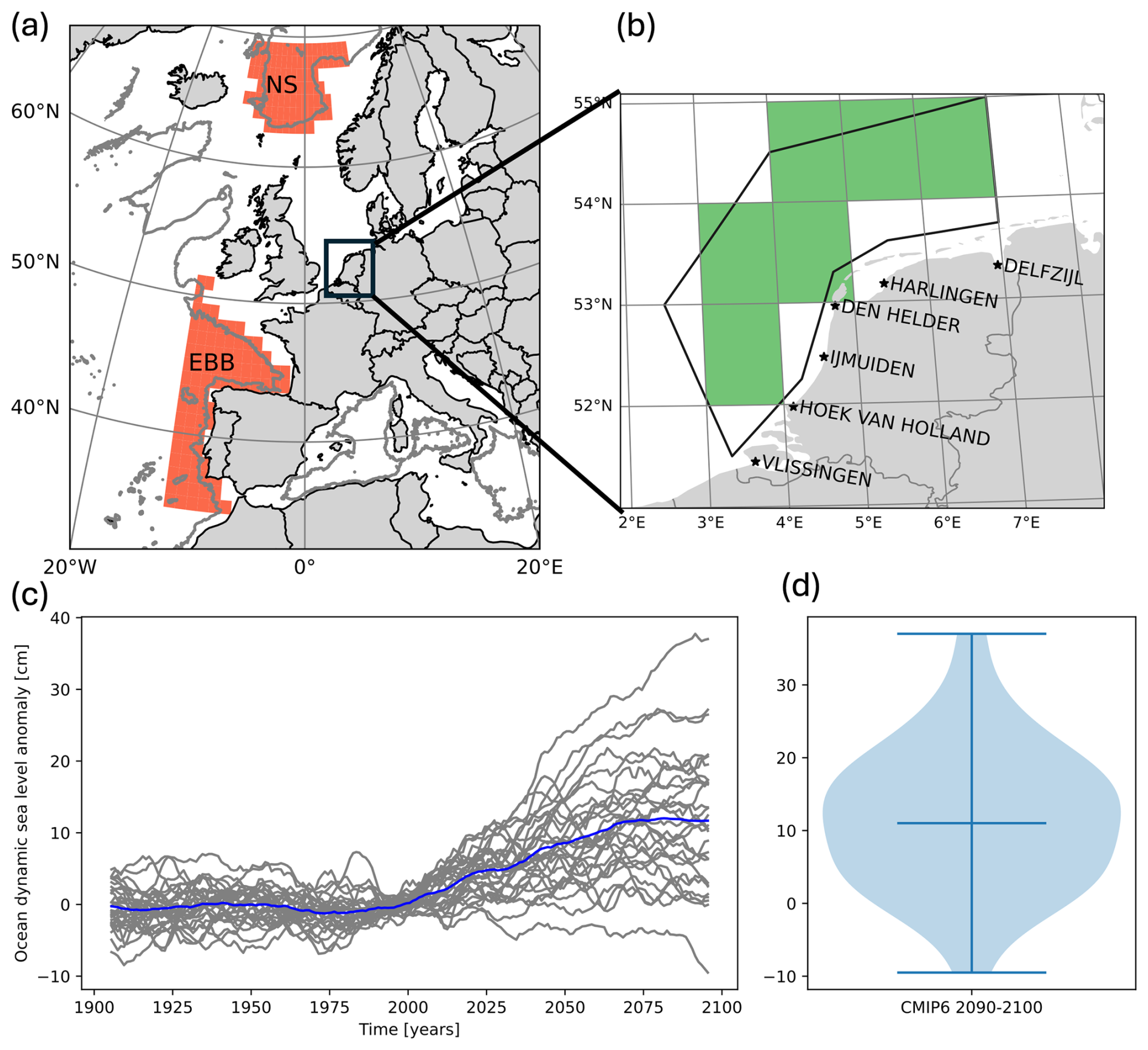
Figure 1(a) The 2000 m isobath and the two regions of steric sea-level change computation: Norwegian Sea (NS) and extended Bay of Biscay (EBB). (b) Location and name of the six reference tide gauges along the Dutch coast. Horizontal grid (1°×1°) on which the CMIP5 and CMIP6 model data are interpolated and the six grid boxes used to compute the local ODSL (green). Region used to compute sea-level rise from satellite altimetry and the SODA ocean reanalysis (black polygon). (c) Changes in ODSL for 29 CMIP6 models under the SSP1-2.6 scenario with the reference period 1986–2005 and a 10-year running average applied. (d) Violin plot showing the distribution of ODSL values averaged over the period 2090–2099 for the same models shown in (c).
2.2 Sea-level budget closure
Another way to estimate ODSL is to consider it as the unknown in the sea-level budget. We develop two budgets for the coast of the Netherlands. The first one is based on geocentric sea-level observations from satellite altimetry data averaged over a region close to the coast (polygon in Fig. 1b). The second one is based on relative sea-level observations from the six reference tide gauges (Vlissingen, Hoek van Holland, IJmuiden, Den Helder, Harlingen, Delfzijl) distributed along the Dutch coast (Keizer et al., 2023). We use ice sheets, glaciers, land water storage, and global steric contributions from the budget of Frederikse et al. (2020a), which considers gravitation, rotation, and viscoelastic deformation effects for all contributions except for global steric sea-level change. Since this budget stops in 2018 we extrapolate the contributions up to 2021 using a linear fit to the last 10 years of the individual time series. This is possible because those terms are rather smooth, and because at the inter-annual timescale, local sea-level change in the North Sea is mostly set by wind (Keizer et al., 2023) and regional steric anomalies (Frederikse et al., 2016). We also include glacial isostatic adjustment from the ICE-6G (VM5a) model (Peltier et al., 2015). The direct influence of the nodal cycle is assumed to be in equilibrium with the astronomical forcing and is calculated as in Woodworth (2012), which was shown to be a good method when the nodal cycle influences on steric effects are considered separately, as we do here (Bult et al., 2024). Once all known sources of sea-level change above are computed, they are removed from the observed sea level, and the effect of wind and inverse barometer on sea level are computed from a multi-linear regression to zonal and meridional wind and pressure fields from the ERA5 reanalysis with the same method as Frederikse et al. (2016).
2.3 Ocean reanalysis
Ocean model reanalyses that assimilate observations of temperature and salinity in a dynamical ocean model also provide an estimate of ODSL. In ocean reanalyses, the relation between the deep ocean and the shelf is computed in a physically consistent manner with the drawback that there is no global ocean reanalysis product yet available that have both the physical mechanisms (e.g. tides) and horizontal resolution necessary to compute the transition between the deep ocean and the shelf (Holt et al., 2017). Some models also assimilate data from satellite altimetry, which includes the influence of other contributors on sea level and makes it difficult to know if the output of the reanalysis is ODSL or geocentric sea level. We use here the Simple Ocean Data Assimilation (SODA3.4.2; Carton et al., 2018), which does not assimilate altimetry data. The data cover the period 1980 to 2020 and have a resolution of 0.5°×0.5° and 50 vertical levels on a Mercator grid. Atmospheric surface forcing is from ERA-interim, and the COARE4 bulk formula is used. To make sure to obtain ODSL from the model output, the global mean sea level is removed for each year. The wind influence is also removed using a multi-linear regression between ODSL and zonal and meridional wind from ERA-interim.
2.4 ODSL from CMIP5 and CMIP6 models
Changes in ODSL are available from the output of the models taking part in CMIP5 and CMIP6 with the variable “zos” but need to be post-processed. We use here the same data as Jesse et al. (2024). The zos variable has three dimensions: time, latitude, and longitude. Four post-processing steps are applied: first, we compute the yearly average from the monthly data. Second, we compute the linear temporal drift in the piControl simulations of each model and remove it from the historical and future scenario simulations for each grid box. This relies on the assumption that the drift is not sensitive to the external forcing (Hobbs et al., 2016). Third, since all models discretize the ocean on different grids, the data are regridded to a common grid. We choose a regular 1°×1° grid. The re-gridding is performed in a computationally efficient way by using the open-source library xESMF with a bilinear method for most models and a nearest-neighbour method for the few models for which the bilinear approach does not work. Additionally, since the land–sea mask is different between models we perform a spatial extrapolation of the available data to where there are no data. This makes sure that all models have data on the same areas. Fourth, we remove the global mean. For CMIP6 models we also remove the influence of local wind on sea level along the coast of the Netherlands to reduce the influence of natural variability on our results.
To estimate the influence of natural variability on the linear trend over 29 years, we use the historical simulations of each model between 1850 and 1980. We assume that before 1980 the anthropogenic trend is not dominating the trend. Using those 131 years, linear trends are computed starting each year. The standard deviation of those 102 trends is used as an indication of the influence of natural variability.
2.5 Wind influence on ODSL from CMIP6 models
The wind influence on ODSL from climate models is computed with a multi-linear regression as for satellite and tide gauge data. However, only the zonal and meridional wind are used in the regression. The atmospheric pressure is not used because the zos variable of climate models does not include the inverse barometer effect (Gregory et al., 2019). Wind and ODSL are selected in a region along the Dutch coast (Fig. 1b). To avoid issues with long-term trend influencing the regression coefficients, we include a linear trend in the regression model and determine the regression coefficients only on the historical period. The assumption that the trend is linear does not hold for the combination of historical and scenario period, but over the historical period it is reasonable. We then assume that the coefficients relating zonal and meridional wind constituents to ODSL obtained during the historical period also apply to the scenario period. More details about the method and analysis of the results can be found in Keizer (2022).
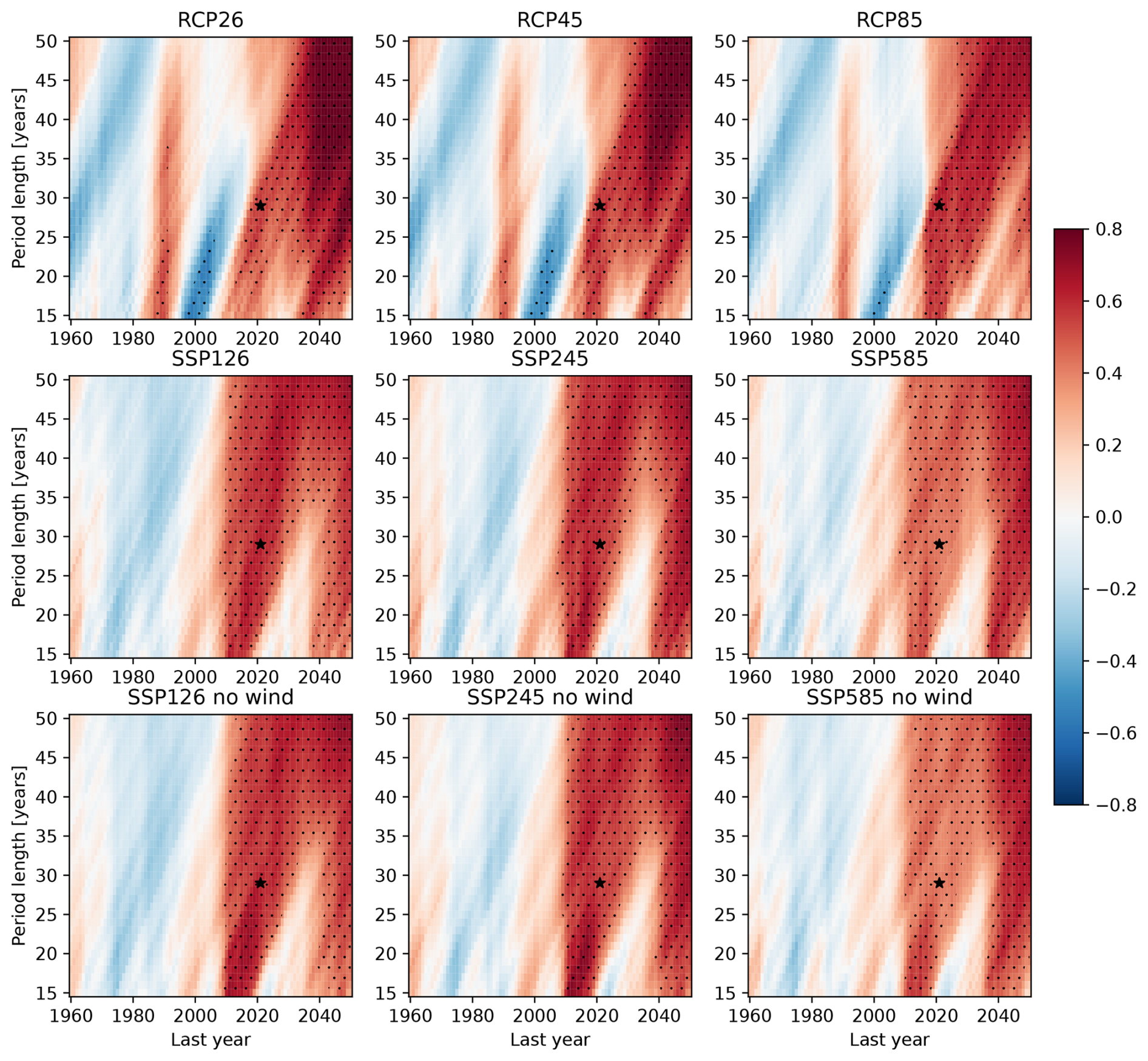
Figure 2Pearson correlation coefficients between rate of ODSL computed for different periods before 2050 and average height anomaly in the period 2090–2099. The columns represent different emission scenarios, and the rows show CMIP5, CMIP6, and CMIP6 with wind corrected, respectively. The last year of the period used to compute the rate varies with the x axis, and the total period length varies with the y axis. The black stars in all panels represent the period ending in 2021 with a length of 29 years, which is 1993–2021. Statistically significant values (p value less than 0.05) are stippled.
In Fig. 1c and d we show the projections of ODSL for the SSP1-2.6 emission scenario of the CMIP6 models along the coast of the Netherlands. There is a large spread between climate models, even for this low emission scenario. For the average of 2090–2099 the values go from −9.5 cm for the FGOALS-g3 model to 37 cm for CIESM. We now investigate if observed ODSL rates of change can be used as a constraint for future ODSL changes. To do that, we look at the relation between, on the one hand, the rate of sea-level rise in the recent past or near future and, on the other hand, the sea-level change between the end of the century 2090–2099 and the reference period 1986–2005 (Fig. 2). We computed the rate of sea-level rise for periods between 15 and 50 years (y axis) ending between 1960 and 2050 for both CMIP5 (top row) and CMIP6 (middle row) models. We see that for rates computed over shorter period the correlation coefficient depends more strongly on the end date of the period than for rates computed over longer periods. This is especially the case for the CMIP5 ensemble with positive correlations for periods ending in 1980 followed by negative correlations for periods ending around 2000 and again positive correlation for periods ending later. Removing wind influence on sea level (third row of Fig. 2) has a limited influence on reducing the variability in the correlation. For the CMIP6 ensemble the correlations are higher for the low emission scenarios (SSP1-2.6, SSP2-4.5) than for the high emission scenario (SSP5-85), which might indicate that different physical mechanisms play a role in the high emission scenario. For the CMIP5 ensemble it is also the case for periods ending after 2030 but not before. In the CMIP6 ensemble there is a sharp increased correlation around 2010 for all period lengths. This could be because the AMOC in CMIP6 models is dominated by internal variability up until around 1990, after which a sharp decline sets in (Fox-Kemper et al., 2021). It could take about 20 years for the AMOC decline to start dominating ODSL changes in the North Sea. We want to select a period that overlaps with the altimetry period that started in 1993 that is as long as possible to reduce the influence of natural variability on the estimation of the trend and that shows significant correlation between the past trend and end-of-century height for both CMIP5 and CMIP6 and for all emission scenarios. We find that for both model ensembles the rate over the full satellite altimetry period 1993–2021 with a length of 29 years provides reasonably high correlation coefficients. For this period the correlation coefficients are 0.54, 0.57, and 0.61 respectively for RCP2.6, RCP4.5, and RCP8.5 and 0.63, 0.57, and 0.42 for SSP1-2.6, SSP2-4.5, and SSP5-85. These coefficients are all significant. The null hypothesis of no-correlation is rejected with a p value between 0.0005 and 0.03. This period is therefore selected for further analysis.
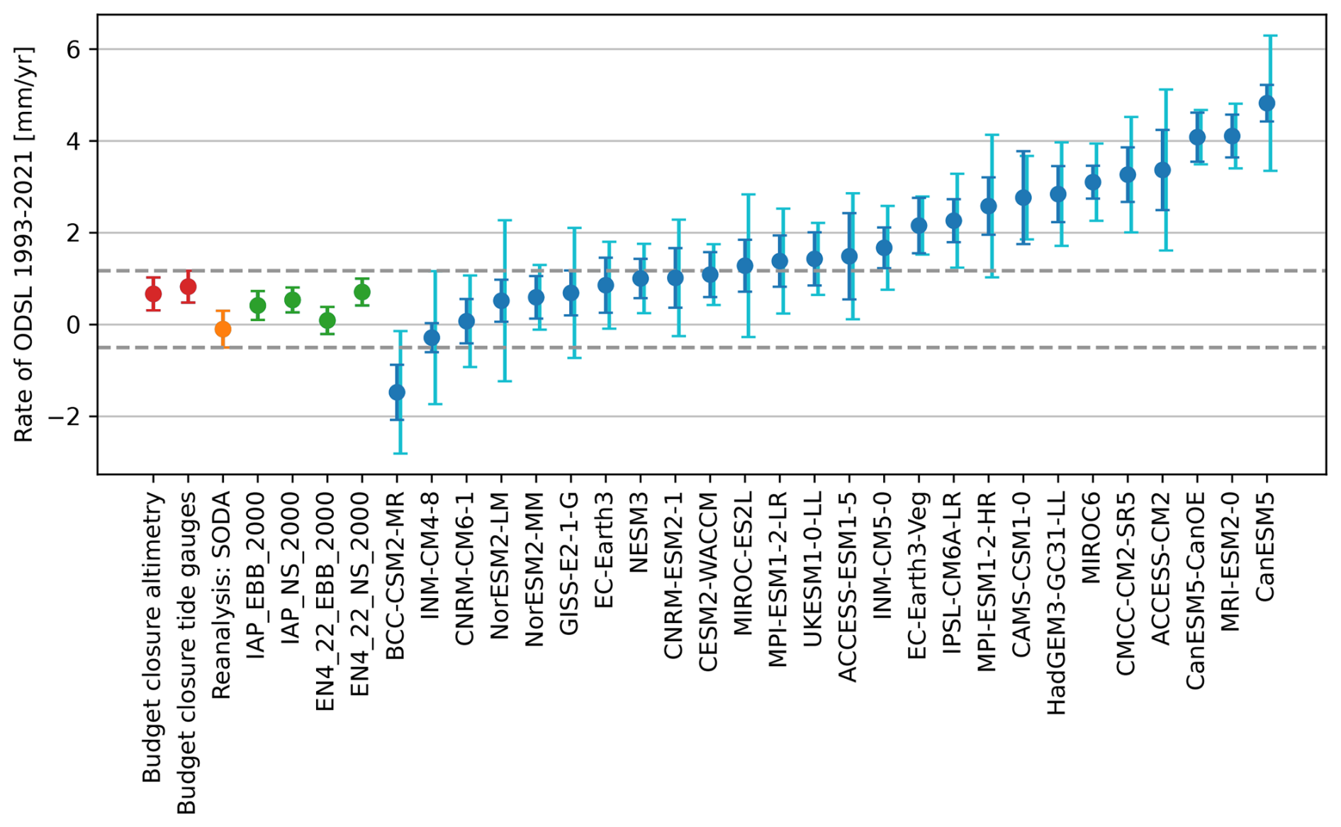
Figure 3Rate of ODSL over the period 1993–2021 obtained from different observational methods and CMIP6 models after wind correction (blue). The slopes for CMIP6 models are computed from the historical experiment up to 2014 and SSP2-4.5 from 2015 to 2021. Budget closure based on tide gauge and satellite altimetry data (red), SODA ocean reanalysis (yellow), and steric sea level in the top 2000 m of the ocean from two different temperature and salt databases (IAP, EN4) and two different regions (EBB, NS; see Fig. 1). The horizontal dashed lines represent the upper and lower values from observational estimates used to select models. The uncertainty ranges show ±1 SD (standard deviation) in the estimation of the rate by fitting a linear trend to the data. For the CMIP6 models, an additional uncertainty range is shown (cyan), also ±1 SD, but based on the natural variability in the historical simulations.
We define three observationally based estimates of ODSL to select the best CMIP6 models for sea-level scenarios. We compute ODSL as the difference between observations and the sum of the other known contributions to sea-level change. We apply this method to a relative sea-level budget based on the measurement from six tide gauges and to a geocentric sea-level budget based on satellite altimetry region along the coast of the Netherlands (Fig. 1b). These two budgets, even though they are based on different observations, provide similar estimates of ODSL trend over the period 1993–2021: 0.8±0.3 and 0.7±0.4 mm yr−1 respectively for the tide gauge and altimetry budgets (red dots in Fig. 3). We now assume that the regional steric sea-level change in the deep ocean around the continental shelf makes its way onto the shelf. Using two different regions and two different gridded observational products and integrating steric anomalies down to a depth of 2000 m, we obtain four estimates of ODSL change (green dots in Fig. 3). The lowest estimate is obtained from EN4 in the extended Bay of Biscay (0.1±0.3 mm yr−1), and the highest is obtained from EN4 in the Norwegian Sea (0.7±0.3 mm yr−1). To avoid the strict assumption that steric sea-level anomalies in the deep ocean close to the shelf have a direct influence on the shelf, we also use an ocean reanalysis. The SODA reanalysis provides a trend of mm yr−1 for the period 1993–2020 (yellow dot in Fig. 3).
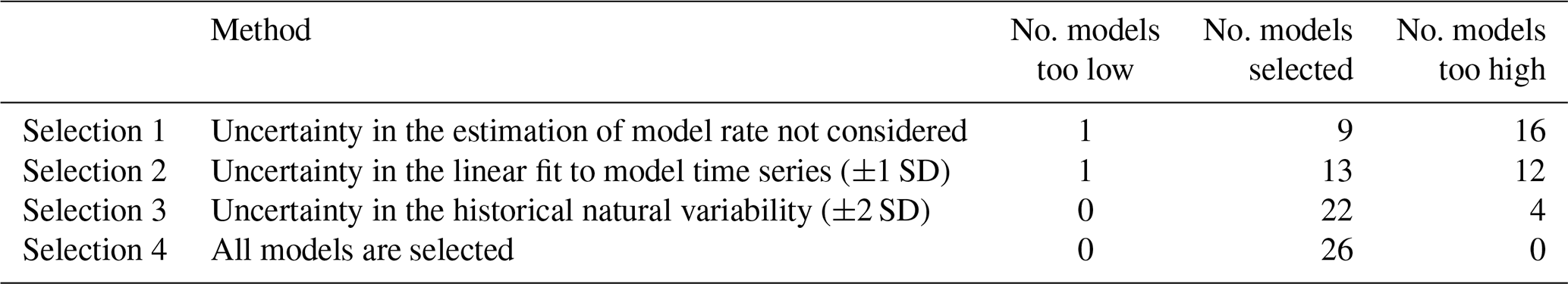
We also compute the ODSL trend from CMIP6 climate models for the average of the six grid boxes shown in Fig. 1b. The wind influence on sea level is removed before computing the rate to reduce the influence of natural climate variability. The rate of ODSL change for the period 1993–2021 goes from −1.5 mm yr−1 for BCC-CSM2-MR to 4.8 mm yr−1 for CanESM5. Even after removing wind influence on sea level and considering a long period of 29 years, part of this broad range might be due to natural climate variability. The Atlantic multidecadal variability could play a role for example (Frankcombe and Dijkstra, 2009). However, since we showed that there is a significant correlation between rates of ODSL change over this period and end-of-the-century change, the range is also determined by specific sensitivity of the ODSL to climate change in those models. We now select models with a realistic ODSL rate. We define a broad observational range of realistic ODSL rate that goes from the lowest observational estimate minus 1 standard error (e.g. −0.5 mm yr−1) up to the highest plus 1 standard error (e.g. 1.2 mm yr−1). Using this observational range, we define four model selections:from the strictest (selection 1) to no selection at all (selection 4) (Table 1). For the first selection, we require that a model rate falls in the observational range without taking the uncertainty in the model rate into account. For the second selection, we consider the uncertainty in fitting a linear trend to the model data (dark-blue range in Fig. 3), and we require that the uncertainty range of the model rate has some overlap with the observational range. For the third selection, we use the uncertainty in the rate computed from the historical simulations. This includes the influence of natural variability. The uncertainty in the rate estimation is larger for this method. The ±1 SD (standard deviation) ranges are shown in Fig. 3. To have an even larger uncertainty range, and because using ±1 SD is somewhat arbitrary, we select the ±2 SD range. For selection 4 all models are selected. Those four selections provide a broad range of potential choices.
Table 1Method of selection and number of models with a rate that is too low, selected, and with a rate that is too high for the four methods.
As the selection becomes less strict, more and more models with high rates are selected. This results in the ensemble average having a rate above the observational range for selection 3 and 4 (Fig. 4). For stricter selections the model ensemble average rates are at the high end of the observational range. The selection also has an influence on the ODSL height at the end of the century. For stricter selection the ensemble ranges are narrower, and the ensemble means are lower.
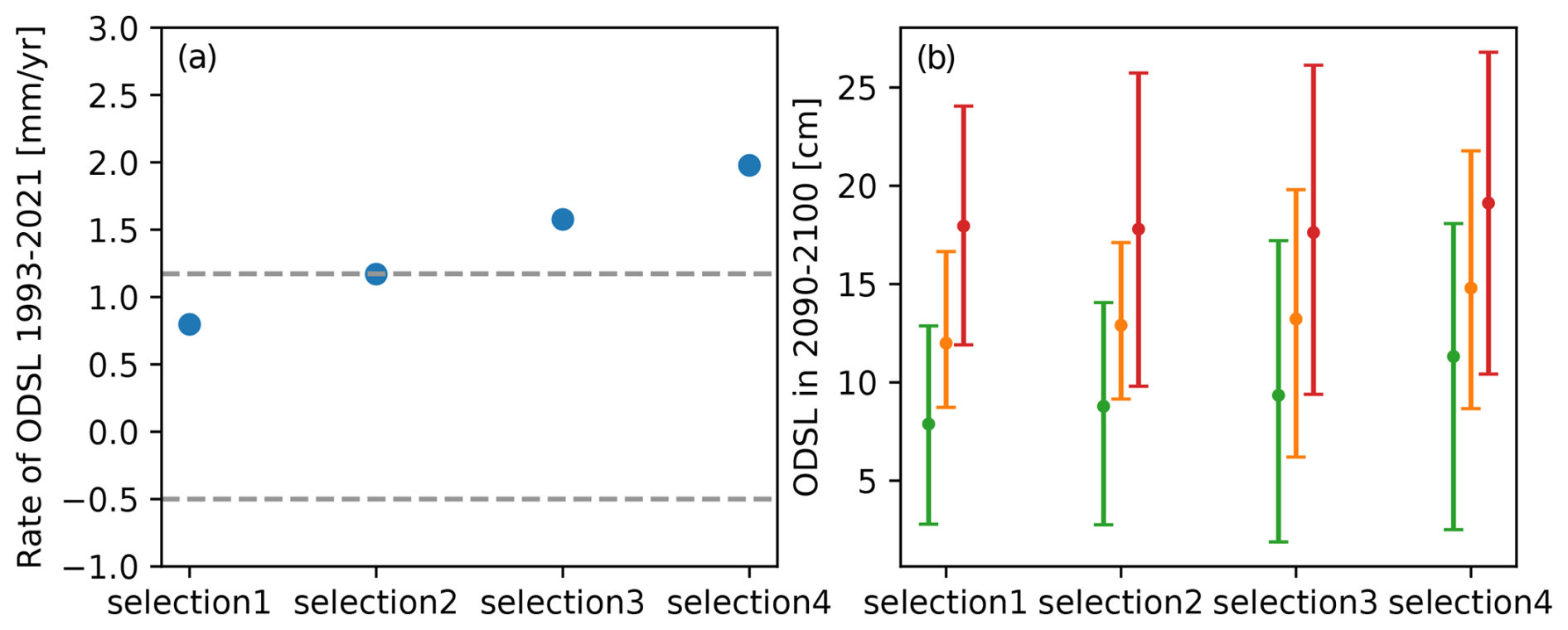
Figure 4Panel (a) shows the ensemble average rate of ODSL for the period 1993–2021 (mm yr−1) for the four CMIP6 model selections. The horizontal dashed lines represent the upper and lower values from observational estimates. Panel (b) shows the height of ODSL (mean and 17th–83rd percentile range) over the period 2090–2099 compared to the reference period 1986–2005. The three emission scenarios are shown for each selection: SSP1-2.6 (green), SSP2-4.5 (orange), and SSP5-8.5 (red).
We now compare selection 2 and 4 in more detail with time series (Fig. 5). The difference is larger for SSP1-2.6 than for SSP5-8.5. This is consistent with the fact that for CMIP6 the correlation between rates over the period 1993–2021 and the height at the end of the century is larger for low emission scenarios. For SSP1-2.6 in 2090–2099, the projection for the ensemble of all models is 12 cm with 17th and 83rd percentiles [2–20], while it is 9 [2–14] cm for the model selection. The influence of model selection is especially large for the 83rd percentile.
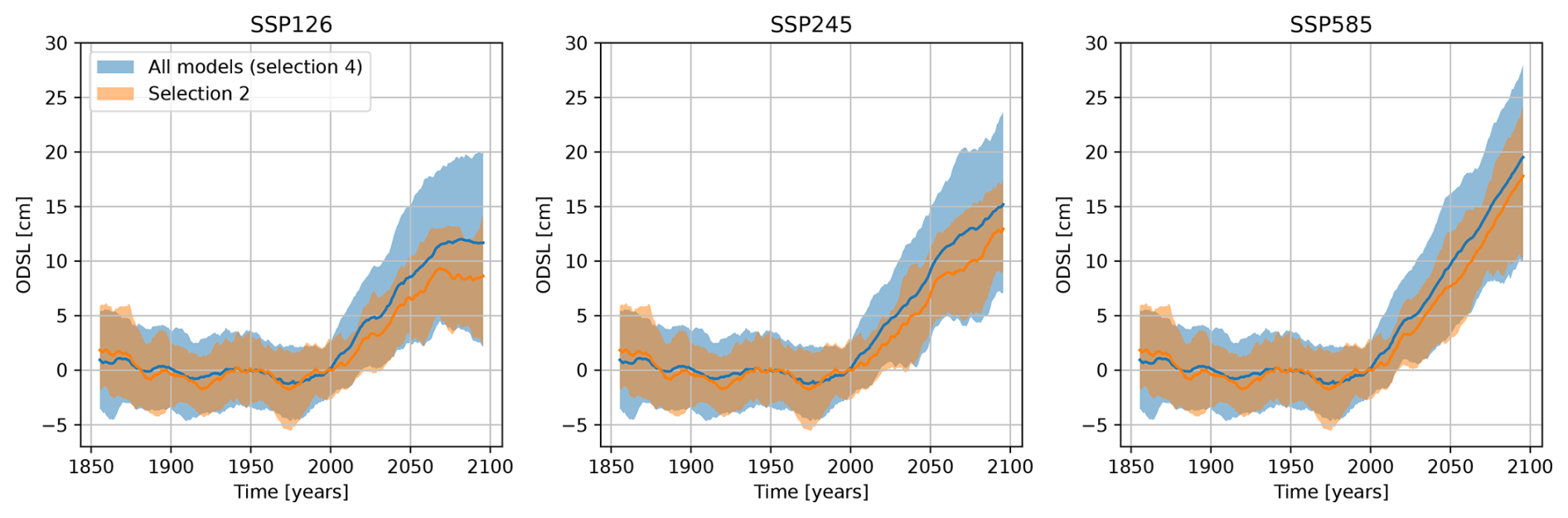
Figure 5Time series of ODSL for the full CMIP6 model ensemble (blue) and for the selection of 13 plausible models based on observations (selection 2, orange). A running average of 10 years is applied. The means and 17th to 83rd percentile ranges are shown.
While ODSL from CMIP models is used extensively for sea-level projections (Church et al., 2013; Fox-Kemper et al., 2021), there are many limitations that need to be kept in mind. Since a dynamical Greenland ice sheet is not yet included in standard AOGCMs, the influence of freshwater from Greenland melt on ODSL changes are not included in our results. Those effects are both direct and indirect. Fresh water is less dense than ocean water, and therefore it raises ODSL locally. The important indirect effect is through a slowdown of the AMOC. The combination of both effects was estimated to be around 5 cm in the North Sea for the 21st century in the Community Earth System Model (Slangen and Lenaerts, 2016). Based on this study, a rough high-end estimate of Greenland melt influence on ODSL for the period 1993–2021 is 0.5 mm yr−1. Since many CMIP6 models already overestimate ODSL, adding this effect would bring them even further from the observational range.
Another physical process missing in the CMIP models is the nodal cycle, with a period of 18.6 years, which was shown to influence steric sea level in the extended Bay of Biscay region and sea level along the western European coast (Bult et al., 2024). Since the period considered here (1993–2021) starts at a low point of the nodal cycle effect on sea level, it could have contributed to 0.16 mm yr−1 ODSL change in the observations. This is a relatively small influence compared to the broad range of uncertainty that we consider, but including this effect in the CMIP models would make them even further from the observed range.
While we consider the gravitation, rotation, and viscoelastic deformation of changes in mass distribution resulting from land ice melt, changes in land water storage, and GIA in the sea-level budget, we do not consider the self-attraction and loading effect of ODSL itself. This effect is present in the observational range but not in the CMIP models. It was estimated to be around 10 % of ODSL in the North Sea (Richter et al., 2013). Again, this effect is relatively small compared to the ranges we have investigated in this study, but taking it into account would make ODSL changes 10 % larger in CMIP models and bring them further from the observations.
The horizontal resolution and related coarse bottom topography of CMIP models is also a limitation. For the North Sea, a particularly important feature is the English Channel. In a downscaling of a model with a closed English Channel, Hermans et al. (2020) showed that ODSL changes are reduced by around 10 cm with a proper representation of the English Channel. However, in the CMIP6 ensemble there is no difference in the mean ODSL change in models with open and closed English Channel. More research is needed on the influence of potential systematic biases due to the coarse resolution of the ocean model part of AOGCMs.
We found a large overestimation of ODSL change in CMIP6 compared to observations over the period 1993–2021. We estimate this overestimation to be about a factor of 3, with a large uncertainty, using the centre of the observational range and the CMIP6 ensemble mean. A few processes might be contributing to this overestimation. First, there is an overestimation of climate sensitivity in the CMIP6 ensemble mean (Zelinka et al., 2020). Second, the poleward bias of maximum westerly winds in the North Atlantic in CMIP6 models was associated with a larger ODSL rise (Lyu et al., 2020). Third, in CMIP6 models the AMOC reaches a maximum in the 1980s followed by a sharp decrease which was not there in CMIP5 and does not seem to be in proxy reconstructions either (Weijer et al., 2020). This could be due to an overestimated sensitivity to aerosol forcing (Robson et al., 2022). A fourth process can be inferred from the results of Jesse et al. (2024). In that study ODSL changes in the North Sea from CMIP models are fitted with a multilinear regression model with global surface air temperature and the AMOC as regressors. On the one hand, we find that CMIP6 models with an overestimated rate of ODSL according to selection 2 have a sensitivity to AMOC change that is 2 times larger than those that are in the plausible range. One sverdrup of AMOC decrease at 35° N results in 2 cm of ODSL rise instead of 1 cm. On the other hand, those models have a sensitivity to global surface air temperature that is half of that of the plausible models; for example, 1 °C warming results in 1.4 cm ODSL rise instead of 2.7 cm. The higher sensitivity of ODSL to AMOC in some CMIP models was explained by the location of deep convection in the North Atlantic (Jesse et al., 2024). In models with a deep convection mostly in the Greenland Sea, a reduced AMOC will raise sea level in the North Sea more than in models with a deep convection in the Irminger Sea or Labrador Sea. A fifth potential explanation for the overestimation of ODSL by CMIP6 is that internal variability would have played a role in slowing down sea-level rise during the period 1993–2021. This could be argued for the period 1993–2012 based the results of Richter et al. (2017), who showed that CMIP5 models are able to produce the same pattern of ODSL change as observed in the North Atlantic but not necessarily for the same period. So far, no study has shown that this was the case for the longer period 1993–2021.
The large range of the ODSL trend from observations (−0.5 to 1.2 mm yr−1) also shows the difficulty in estimating this quantity from observations, especially for shelf seas. The three methods we used have important limitations. Using ODSL as the unknown in the sea-level budget makes its estimation dependent on being able to quantify all other components of the budget with a good accuracy. Using the steric sea level in the deep ocean relies on the questionable assumption that there is no horizontal pressure gradient between the deep ocean and the shelf. Bingham and Hughes (2012) suggest that choosing regions closer to the coast and less deep integration results in better correlation between steric sea level and coastal sea level at an inter-annual timescale. However, we look at a longer timescale, so it is not clear how their conclusion applies to our study. We look at the difference in Fig. A1 between an integration down to 500 and 2000 m. The results show that for both IAP and EN4 the choice of integration down to 500 m would result in a smaller rate of steric sea level rise and would not change the range we have now for the observed ODSL rate. Ocean reanalyses have the potential to solve those issues and be the best tool to diagnose ODSL along the shelf but still suffer from issues like drifts and biases due to air–sea fluxes, ocean mixing errors, coarse model resolution, or the assimilation of observations (Dangendorf et al., 2021).
We have used the period 1993–2021 (29 years) to select models, the longest period for which satellite altimetry is available. For selection 2 we found that 13 models were selected. For shorter periods the number of models selected is larger because the uncertainty in computing the rate of sea-level rise from both observations and models is larger. For the periods 1993–2007 (15 years), 1993–2012 (20 years), and 1993–2017 (25 years), the numbers of models selected are 24, 19, and 15 respectively. Out of a total of 26 models, the model selection also depends on the exact period used. For example, while 15 models are selected for the period 1993–2017, for the period 1997–2021, which is also 25 years, only 12 models are selected. One model has a rate that is too low to be selected, the same for both periods. The number of models with a rate that is too high is 10 for 1993–2017 and 13 for 1997–2021 with 9 overlapping models.
Given the complexity of ODSL changes, the physical limitations and biases of AOGCMs discussed above, and the different goals of projections, it is difficult to say which one of the four selections presented here should be used. On the one hand we argue that, in the absence of a good understanding of natural variability of sea level in the North Sea, making projections of ODSL with models that are far away from the observational range as in selections 3 and 4 reduces the trust in the projections (Wang et al., 2021). Therefore, we advise most users of sea level projections to use method 1 or 2. On the other hand, AOGCMs could be selected because of compensating biases. For example, they could have the right past ODSL rate for the wrong reason and therefore do not provide better projections. Additionally, for users of sea-level projections who are risk-averse, the risk of not selecting models that could provide important information about the future and underestimating future ODSL as a result is not acceptable. In that case, selection 3 or 4 would be better suited. In any case, more work needs to be done to understand and evaluate AOGCMs over multidecadal periods, which is less than the typical centennial timescale they are usually used for.
This study focused on the coast of the Netherlands, which is part of the North Sea. However, the method could be more broadly applied. Given the smoothness of mean ODSL projections from CMIP models, we would expect similar results for the whole western European coast. For other regions around the world, the results will be different, but the method we developed here would also apply. Estimating ODSL from observations would be easier in places with a narrower shelf; the uncertainty related to physical mechanisms transforming the steric sea-level change from the deep ocean to manometric sea-level change on the shelf would be reduced (Bingham and Hughes, 2012). The satellite data that we use to estimate ODSL changes are available everywhere around the world, but the number of good-quality, continuous tide gauge measurements is exceptional along the Dutch coast.
To improve projections of ODSL changes for the coast of the Netherlands based on CMIP6 AOGCMs, we looked at the potential for the rate of change for past periods to inform about the height at the end of the century. We found that rates computed over the period 1993–2021 correlate significantly with height at the end of the century. However, correlation coefficients are around 0.4 to 0.6, depending on the CMIP version and the emission scenario, showing that different processes also play a role in driving the spread of ODSL height at the end of the century.
We then estimated ODSL change for the period 1993-2021 with three different methods. The first method assumes that ODSL is the difference between observed sea level and the sum of all known contributors to sea-level rise, e.g. ice sheets, glaciers, land water storage, global steric sea level, and glacial isostatic adjustment. We applied this method to both relative sea level from tide gauges and geocentric sea level from satellite altimetry. In the second method we computed regional steric sea-level change in two regions of the deep ocean outside of the North Sea: the extended Bay of Biscay and the Norwegian Sea. In the third method we used sea-level data from an ocean reanalysis that does not assimilate satellite altimetry data. These three methods provide seven estimates of ODSL rates of change during the period 1993–2021. Based on these estimates we defined a broad range of plausible values: [−0.5, 1.2] mm yr−1.
This range was compared to the rates of CMIP6 models from which the influence of local wind variability was removed. We found that 4 to 16 models simulate a rate that falls above this range depending on how the uncertainty in the rate of AOGCM is considered. We define four selection methods ranging from a very strict method that requires that the rate of an AOGCM falls in the observational range without considering the uncertainty in the rate estimation (selection 1) to using all AOGCMs (selection 4). Selecting models results in a lower ensemble mean and narrower uncertainty ranges at the end of the century. The difference is largest for the low emission scenario SSP1-2.6 for which the median and 83rd percentiles are reduced by about 25 % in selection 2 compared to using all AOGCMs. We argue that using a strict selection method (selection 1 or 2) is better for most users except for risk-averse users who could consider selection 3 or 4. We discussed a few reasons that could explain the large overestimation of many models. An overestimation of the sensitivity of the local ODSL changes to AMOC changes seems to be playing an important role.
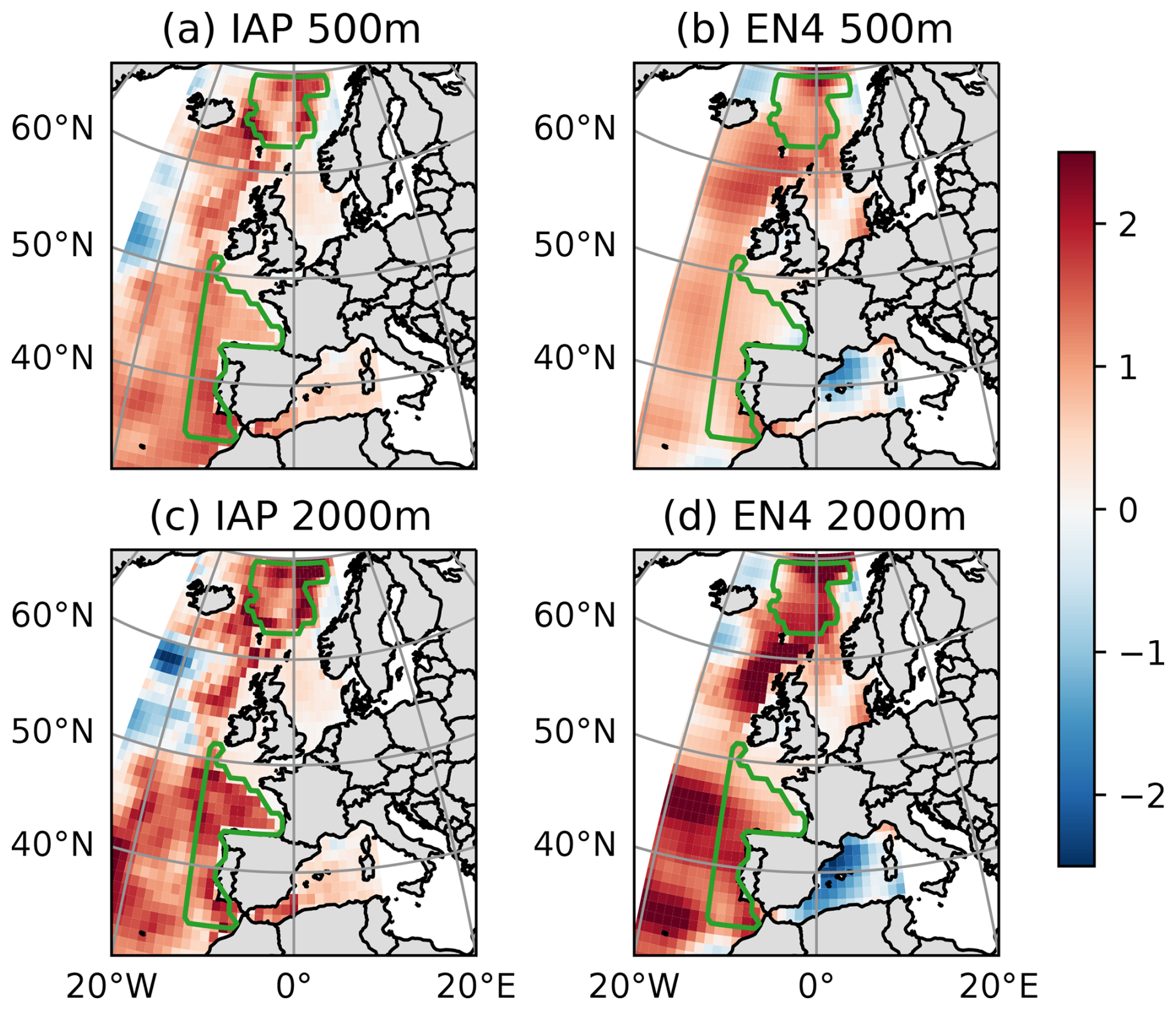
Figure A1Maps of rate of vertically integrated steric sea-level change in mm yr−1 from the surface to 500 m depth (a, b) and from the surface to 2000 m depth (c, d): (a, c) is for IAP and (b, d) for EN4. Green contours indicate the Norwegian Sea and the extended Bay of Biscay regions.
The EN.4.2.2 data were obtained from https://www.metoffice.gov.uk/hadobs/en4/ (Met Office, 2025) and have a British Crown copyright, Met Office, provided under a non-commercial government licence (http://www.nationalarchives.gov.uk/doc/non-commercial-government-licence/version/2/, last access: 11 July 2025). To compute ocean density, we used the GSW-Python toolbox at https://teos-10.github.io/GSW-Python/install.html (TEOS-10 developers, 2025). The budget data from Frederikse et al. (2020a) can be downloaded at https://doi.org/10.5281/zenodo.3862995 (Frederikse et al., 2020b). The ICE6G data are available at https://www.atmosp.physics.utoronto.ca/~peltier/data.php (Peltier, 2025). The ERA5 data are available from the Climate Data Store at https://doi.org/10.24381/cds.f17050d7 (Hersbach et al., 2023). The code developed to compute the sea-level budget is available on Zenodo at https://doi.org/10.5281/zenodo.14046697 (Le Bars, 2024). The SODA 3.4.2 data can be found at https://dsrs.atmos.umd.edu/DATA/soda3.4.2/REGRIDED/ocean/ (Carton et al., 2025). The code developed to analyse the SODA data is available on Zenodo at https://doi.org/10.5281/zenodo.15854062 (Keizer, 2025). The output from CMIP6 climate models is available from the Earth System Grid Federation (ESGF) CMIP6 search interface (https://esgf-node.ipsl.upmc.fr/search/cmip6-ipsl/, Earth System Grid Federation, 2025). The code developed to compute the wind influence on CMIP6 ODSL is available on Zenodo at https://doi.org/10.5281/zenodo.15854069 (Keizer, 2025b). The code developed for the data analysis and figure production is available on Zenodo at https://doi.org/10.5281/zenodo.15799703 (Le Bars, 2025) under the GPL-3.0 licence.
DLB and SD conceptualized the study. DLB and IK performed the data analysis. DLB wrote the first draft. All authors contributed to the preparation of the final draft.
The contact author has declared that none of the authors has any competing interests.
Publisher's note: Copernicus Publications remains neutral with regard to jurisdictional claims made in the text, published maps, institutional affiliations, or any other geographical representation in this paper. While Copernicus Publications makes every effort to include appropriate place names, the final responsibility lies with the authors.
We would like to thank Franka Jesse for providing the regression coefficient data from Jesse et al. (2024). This study was part of the development of the new KNMI'23 sea-level scenarios for the coast of the Netherlands. We thank the two anonymous reviewers for their comments that considerably improved this work.
This publication was supported by the Knowledge Programme Sea Level Rise, which received funding from the Dutch Ministry of Infrastructure and Water Management, and PROTECT, which received funding from the European Union's Horizon 2020 research and innovation programme (grant no. 869304) (PROTECT contribution number 157).
This paper was edited by Meric Srokosz and reviewed by two anonymous referees.
Bingham, R. J. and Hughes, C. W.: Local diagnostics to estimate density-induced sea level variations over topography and along coastlines: topography and sea level, J. Geophys. Res.-Oceans, 117, C01013, https://doi.org/10.1029/2011JC007276, 2012.
Bulgin, C. E., Mecking, J. V., Harvey, B. J., Jevrejeva, S., McCarroll, N. F., Merchant, C. J., and Sinha, B.: Dynamic sea-level changes and potential implications for storm surges in the UK: a storylines perspective, Environ. Res. Lett., 18, 044033, https://doi.org/10.1088/1748-9326/acc6df, 2023.
Bult, S. V., Le Bars, D., Haigh, I. D., and Gerkema, T.: The Effect of the 18.6-Year Lunar Nodal Cycle on Steric Sea Level Changes, Geophys. Res. Lett., 51, e2023GL106563, https://doi.org/10.1029/2023GL106563, 2024.
Calafat, F. M., Chambers, D. P., and Tsimplis, M. N.: Mechanisms of decadal sea level variability in the eastern North Atlantic and the Mediterranean Sea, J. Geophys. Res.-Oceans, 117, C09022, https://doi.org/10.1029/2012JC008285, 2012.
Camargo, C. M. L., Riva, R. E. M., Hermans, T. H. J., Schütt, E. M., Marcos, M., Hernandez-Carrasco, I., and Slangen, A. B. A.: Regionalizing the sea-level budget with machine learning techniques, Ocean Sci., 19, 17–41, https://doi.org/10.5194/os-19-17-2023, 2023.
Carton, J. A., Chepurin, G. A., and Chen, L.: SODA3: A New Ocean Climate Reanalysis, J. Climate, 31, 6967–6983, https://doi.org/10.1175/JCLI-D-18-0149.1, 2018.
Carton, J. A., Chepurin, G. A., and Chen, L.: SODA 3.4.2 ocean reanalysis, Department of Atmospheric and Oceanic Science at the University of Maryland [data set], https://dsrs.atmos.umd.edu/DATA/soda3.4.2/REGRIDED/ocean/, last access: 2 July 2025.
Cheng, L., Trenberth, K. E., Fasullo, J., Boyer, T., Abraham, J., and Zhu, J.: Improved estimates of ocean heat content from 1960 to 2015, Sci. Adv., 3, e1601545, https://doi.org/10.1126/sciadv.1601545, 2017.
Church, J. A., Clark, P. U., Cazenave, A., Gregory, J. M., Jevrejeva, S., Levermann, A., Merrifield, M. A., Milne, G. A., Nerem, R. S., Nunn, P. D., Payne, A. J., Pfeffer, W. T., Stammer, D., and Unnikrishnan, A. S.: Sea Level Change, in: Climate Change 2013: The Physical Science Basis, Contribution of Working Group I to the Fifth Assessment Report of the Intergovernmental Panel on Climate Change, edited by: Stocker, T. F., Qin, D., Plattner, G.-K., Tignor, M., Allen, S. K., Boschung, J., Nauels, A., Xia, Y., Bex, V., and Midgley, P. M., Cambridge University Press, Cambridge, UK and New York, NY, USA, https://doi.org/10.1017/CBO9781107415324.026, 2013.
Dangendorf, S., Frederikse, T., Chafik, L., Klinck, J. M., Ezer, T., and Hamlington, B. D.: Data-driven reconstruction reveals large-scale ocean circulation control on coastal sea level, Nat. Clim. Change, 11, 514–520, https://doi.org/10.1038/s41558-021-01046-1, 2021.
DeConto, R. M., Pollard, D., Alley, R. B., Velicogna, I., Gasson, E., Gomez, N., Sadai, S., Condron, A., Gilford, D. M., Ashe, E. L., Kopp, R. E., Li, D., and Dutton, A.: The Paris Climate Agreement and future sea-level rise from Antarctica, Nature, 593, 83–89, https://doi.org/10.1038/s41586-021-03427-0, 2021.
Earth System Grid Federation: ESGF MetaGrid, Earth System Grid Federation [data set], https://esgf-node.ipsl.upmc.fr/search/cmip6-ipsl/, last access: 2 June 2025.
Fox-Kemper, B., Hewitt, H. T., Xiao, C., Aðalgeirsdóttir, G., Drijfhout, S. S., Edwards, T. L., Golledge, N. R., Hemer, M., Kopp, R. E., Krinner, G., Mix, A., Notz, D., Nowicki, S., Nurhati, I. S., Ruiz, L., Sallée, J. B., and Slangen, A. B. A.: Ocean, Cryosphere and Sea Level Change, in: Climate Change 2021: The Physical Science Basis, Contribution of Working Group I to the Sixth Assessment Report of the Intergovernmental Panel on Climate Change, edited by: Masson-Delmotte, V., Zhai, P., Pirani, A., Connors, S. L., Péan, C., Berger, S., Caud, N., Chen, Y., Goldfarb, L., Gomis, M. I., Huang, M., Leitzell, K., Lonnoy, E., Matthews, J. B. R., Maycock, T. K., Waterfield, T., Yelekçi, O., Yu, R., and Zhou, B., Cambridge University Press, https://doi.org/10.1017/9781009157896.011, 2021.
Frankcombe, L. M. and Dijkstra, H. A.: Coherent multidecadal variability in North Atlantic sea level, Geophys. Res. Lett., 36, L15604, https://doi.org/10.1029/2009GL039455, 2009.
Frederikse, T., Riva, R., Kleinherenbrink, M., Wada, Y., van den Broeke, M., and Marzeion, B.: Closing the sea level budget on a regional scale: Trends and variability on the Northwestern European continental shelf, Geophys. Res. Lett., 43, 10864–10872, https://doi.org/10.1002/2016GL070750, 2016.
Frederikse, T., Landerer, F., Caron, L., Adhikari, S., Parkes, D., Humphrey, V. W., Dangendorf, S., Hogarth, P., Zanna, L., Cheng, L., and Wu, Y.-H.: The causes of sea-level rise since 1900, Nature, 584, 393–397, https://doi.org/10.1038/s41586-020-2591-3, 2020a.
Frederikse, T., Landerer, F., Caron, L., Adhikari, S., Parkes, D., Humphrey, V. W., Dangendorf, S., Hogarth, P., Zanna, L., Cheng, L., and Wu, Y.-H.: Data supplement of “The causes of sea-level rise since 1900”, Zenodo [data set], https://doi.org/10.5281/zenodo.3862995, 2020b.
Good, S. A., Martin, M. J., and Rayner, N. A.: EN4: Quality controlled ocean temperature and salinity profiles and monthly objective analyses with uncertainty estimates, J. Geophys. Res.-Oceans, 118, 6704–6716, https://doi.org/10.1002/2013JC009067, 2013.
Gouretski, V. and Reseghetti, F.: On depth and temperature biases in bathythermograph data: Development of a new correction scheme based on analysis of a global ocean database, Deep-Sea Res. Pt. I, 57, 812–833, https://doi.org/10.1016/j.dsr.2010.03.011, 2010.
Gregory, J. M., Griffies, S. M., Hughes, C. W., Lowe, J. A., Church, J. A., Fukimori, I., Gomez, N., Kopp, R. E., Landerer, F., Cozannet, G. L., Ponte, R. M., Stammer, D., Tamisiea, M. E., and van de Wal, R. S. W.: Concepts and Terminology for Sea Level: Mean, Variability and Change, Both Local and Global, Surv. Geophys., 40, 1251–1289, https://doi.org/10.1007/s10712-019-09525-z, 2019.
Hall, A., Cox, P., Huntingford, C., and Klein, S.: Progressing emergent constraints on future climate change, Nat. Clim. Change, 9, 269–278, https://doi.org/10.1038/s41558-019-0436-6, 2019.
Hermans, T. H. J., Tinker, J., Palmer, M. D., Katsman, C. A., Vermeersen, B. L. A., and Slangen, A. B. A.: Improving sea-level projections on the Northwestern European shelf using dynamical downscaling, Clim. Dynam., 54, 1987–2011, https://doi.org/10.1007/s00382-019-05104-5, 2020.
Hersbach, H., Bell, B., Berrisford, P., Biavati, G., Horányi, A., Muñoz Sabater, J., Nicolas, J., Peubey, C., Radu, R., Rozum, I., Schepers, D., Simmons, A., Soci, C., Dee, D., and Thépaut, J.-N.: ERA5 monthly averaged data on single levels from 1940 to present, Copernicus Climate Change Service (C3S) Climate Data Store (CDS) [data set], https://doi.org/10.24381/cds.f17050d7, 2023.
Hinkel, J., Church, J. A., Gregory, J. M., Lambert, E., Le Cozannet, G., Lowe, J., McInnes, K. L., Nicholls, R. J., Pol, T. D., and Wal, R.: Meeting User Needs for Sea Level Rise Information: A Decision Analysis Perspective, Earth's Future, 7, 320–337, https://doi.org/10.1029/2018EF001071, 2019.
Hobbs, W., Palmer, M. D., and Monselesan, D.: An Energy Conservation Analysis of Ocean Drift in the CMIP5 Global Coupled Models, J. Climate, 29, 1639–1653, https://doi.org/10.1175/JCLI-D-15-0477.1, 2016.
Holt, J., Hyder, P., Ashworth, M., Harle, J., Hewitt, H. T., Liu, H., New, A. L., Pickles, S., Porter, A., Popova, E., Allen, J. I., Siddorn, J., and Wood, R.: Prospects for improving the representation of coastal and shelf seas in global ocean models, Geosci. Model Dev., 10, 499–523, https://doi.org/10.5194/gmd-10-499-2017, 2017.
Hughes, C. W., Fukumori, I., Griffies, S. M., Huthnance, J. M., Minobe, S., Spence, P., Thompson, K. R., and Wise, A.: Sea Level and the Role of Coastal Trapped Waves in Mediating the Influence of the Open Ocean on the Coast, Surv. Geophys., 40, 1467–1492, https://doi.org/10.1007/s10712-019-09535-x, 2019.
Huthnance, J., Hopkins, J., Berx, B., Dale, A., Holt, J., Hosegood, P., Inall, M., Jones, S., Loveday, B. R., Miller, P. I., Polton, J., Porter, M., and Spingys, C.: Ocean shelf exchange, NW European shelf seas: Measurements, estimates and comparisons, Prog. Oceanogr., 202, 102760, https://doi.org/10.1016/j.pocean.2022.102760, 2022.
Jesse, F., Le Bars, D., and Drijfhout, S.: Processes explaining increased ocean dynamic sea level in the North Sea in CMIP6, Environ. Res. Lett., 19, 044060, https://doi.org/10.1088/1748-9326/ad33d4, 2024.
Keizer, I.: Long-Term Wind Influence on Sea-Level Change Along the Dutch Coast, Utrecht University, https://studenttheses.uu.nl/handle/20.500.12932/560 (last access: 3 July 2025), 2022.
Keizer, I.: iris-keizer/ROMS-project: ROMS-project, Zenodo [code], https://doi.org/10.5281/zenodo.15854062, 2025a.
Keizer, I.: iris-keizer/Thesis-KNMI: Thesis-KNMI, Zenodo [code], https://doi.org/10.5281/zenodo.15854069, 2025b.
Keizer, I., Le Bars, D., de Valk, C., Jüling, A., van de Wal, R., and Drijfhout, S.: The acceleration of sea-level rise along the coast of the Netherlands started in the 1960s, Ocean Sci., 19, 991–1007, https://doi.org/10.5194/os-19-991-2023, 2023.
Landerer, F. W., Jungclaus, J. H., and Marotzke, J.: Regional Dynamic and Steric Sea Level Change in Response to the IPCC-A1B Scenario, J. Phys. Oceanogr., 37, 296–312, https://doi.org/10.1175/JPO3013.1, 2007.
Le Bars, D.: Uncertainty in Sea Level Rise Projections Due to the Dependence Between Contributors, Earth's Future, 6, 1275–1291, https://doi.org/10.1029/2018EF000849, 2018.
Le Bars, D.: Dlebars/SLBudget: First Release, Zenodo [data set], https://doi.org/10.5281/zenodo.14046697, 2024.
Le Bars, D.: KNMI-sealevel/Obs_ODSL_Netherlands: First release, Zenodo [code], https://doi.org/10.5281/zenodo.15799703, 2025.
Le Cozannet, G., Nicholls, R., Hinkel, J., Sweet, W., McInnes, K., Van de Wal, R., Slangen, A., Lowe, J., and White, K.: Sea Level Change and Coastal Climate Services: The Way Forward, J. Mar. Sci. Eng., 5, 49, https://doi.org/10.3390/jmse5040049, 2017.
Lyu, K., Zhang, X., and Church, J. A.: Regional Dynamic Sea Level Simulated in the CMIP5 and CMIP6 Models: Mean Biases, Future Projections, and Their Linkages, J. Climate, 33, 6377–6398, https://doi.org/10.1175/JCLI-D-19-1029.1, 2020.
Lyu, K., Zhang, X., and Church, J. A.: Projected ocean warming constrained by the ocean observational record, Nat. Clim. Change, 11, 834–839, https://doi.org/10.1038/s41558-021-01151-1, 2021.
Met Office: EN4: quality controlled subsurface ocean temperature and salinity profiles and objective analyses, Met Office [data set], https://www.metoffice.gov.uk/hadobs/en4/, last access: 2 July 2025.
Millero, F. J., Feistel, R., Wright, D. G., and McDougall, T. J.: The composition of Standard Seawater and the definition of the Reference-Composition Salinity Scale, Deep-Sea Res. Pt. I, 55, 50–72, https://doi.org/10.1016/j.dsr.2007.10.001, 2008.
Peltier, W. R.: ICE-6G dataset, University of Toronot [data set], https://www.atmosp.physics.utoronto.ca/~peltier/data.php, last access: 2 July 2025.
Peltier, W. R., Argus, D. F., and Drummond, R.: Space geodesy constrains ice age terminal deglaciation: The global ICE-6G_C (VM5a) model: Global Glacial Isostatic Adjustment, J. Geophys. Res.-Solid, 120, 450–487, https://doi.org/10.1002/2014JB011176, 2015.
Richter, K., Riva, R. E. M., and Drange, H.: Impact of self-attraction and loading effects induced by shelf mass loading on projected regional sea level rise: shelf mass loading and sal effects, Geophys. Res. Lett., 40, 1144–1148, https://doi.org/10.1002/grl.50265, 2013.
Richter, K., Øie Nilsen, J. E., Raj, R. P., Bethke, I., Johannessen, J. A., Slangen, A. B. A., and Marzeion, B.: Northern North Atlantic Sea Level in CMIP5 Climate Models: Evaluation of Mean State, Variability, and Trends against Altimetric Observations, J. Climate, 30, 9383–9398, https://doi.org/10.1175/JCLI-D-17-0310.1, 2017.
Robson, J., Menary, M. B., Sutton, R. T., Mecking, J., Gregory, J. M., Jones, C., Sinha, B., Stevens, D. P., and Wilcox, L. J.: The Role of Anthropogenic Aerosol Forcing in the 1850–1985 Strengthening of the AMOC in CMIP6 Historical Simulations, J. Climate, 35, 6843–6863, https://doi.org/10.1175/JCLI-D-22-0124.1, 2022.
Slangen, A. B. A. and Lenaerts, J. T. M.: The sea level response to ice sheet freshwater forcing in the Community Earth System Model, Environ. Res. Lett., 11, 104002, https://doi.org/10.1088/1748-9326/11/10/104002, 2016.
TEOS-10 developers: Python implementation of the Thermodynamic Equation of Seawater 2010, gsw [code], https://teos-10.github.io/GSW-Python/install.html, last access: 2 July 2025.
van der Linden, E. C., Le Bars, D., Lambert, E., and Drijfhout, S.: Antarctic contribution to future sea level from ice shelf basal melt as constrained by ice discharge observations, The Cryosphere, 17, 79–103, https://doi.org/10.5194/tc-17-79-2023, 2023.
Vries, H. de, Katsman, C., and Drijfhout, S.: Constructing scenarios of regional sea level change using global temperature pathways, Environ. Res. Lett., 9, 115007, https://doi.org/10.1088/1748-9326/9/11/115007, 2014.
Wang, J., Church, J. A., Zhang, X., and Chen, X.: Reconciling global mean and regional sea level change in projections and observations, Nat. Commun., 12, 990, https://doi.org/10.1038/s41467-021-21265-6, 2021.
Weijer, W., Cheng, W., Garuba, O. A., Hu, A., and Nadiga, B. T.: CMIP6 Models Predict Significant 21st Century Decline of the Atlantic Meridional Overturning Circulation, Geophys. Res. Lett., 47, e2019GL086075, https://doi.org/10.1029/2019GL086075, 2020.
Woodworth, P. L.: A Note on the Nodal Tide in Sea Level Records, J. Coast. Res., 28, 316–323, https://doi.org/10.2112/JCOASTRES-D-11A-00023.1, 2012.
Zelinka, M. D., Myers, T. A., McCoy, D. T., Po-Chedley, S., Caldwell, P. M., Ceppi, P., Klein, S. A., and Taylor, K. E.: Causes of Higher Climate Sensitivity in CMIP6 Models, Geophys. Res. Lett., 47, e2019GL085782, https://doi.org/10.1029/2019GL085782, 2020.