Synoptic patterns associated with high-frequency sea level extremes in the Adriatic Sea

This study focuses on the classification of synoptic conditions leading to episodes of extreme high-frequency (HF) sea level oscillations in the Adriatic Sea (Mediterranean). Two types of extreme episodes were obtained from sea level time series measured at six tide gauge stations: (i) HF extremes, extracted from HF components (periods shorter than 2 h) of sea level time series and defined as periods in which the HF component was above a threshold value, and (ii) compound extremes, extracted from residual (de-tided) time series and defined as periods in which both HF and residual components were above their respective thresholds. Characteristic synoptic situations preceding both types of extremes were determined using the k-medoids clustering method applied on the ERA5 reanalysis data (mean sea level pressure, temperature at 850 hPa, and geopotential height of 500 hPa level). The structural similarity index measure (SSIM) was used as a distance metric. The data were divided into a training set (from the start of measurements to the beginning of 2018) and a testing set (from the beginning of 2018 to the end of 2020). For each station, the k-medoids method was used to obtain first two and then three clusters with characteristic synoptic patterns called “medoids”. Two distinct patterns related to HF and compound extremes were identified at all stations: (i) a “summer-type” pattern, characterised by a non-gradient mean sea level pressure, warm air advection from the south-southwest at 850 hPa, and the presence of a jet stream at the 500 hPa height, with all three conditions previously found to favour the development of meteorological tsunamis (i.e.  the strongest of atmospherically triggered HF sea level oscillations); (ii) a “winter-type” pattern, characterised by pronounced mean sea level pressure gradients favouring winds that induce storm surges, a colder low troposphere, and the presence of a jet stream at the 500 hPa level. Including the third cluster in the analysis led to the extraction of either a novel “bora-type” pattern, involving strong northeast winds at the Bakar and Rovinj stations, or an additional cluster with a medoid that represents the refinement of summer- or winter-type patterns. The extracted medoids of clusters were used to label all days of the testing period. It was shown that HF or compound episodes recorded in the testing period mostly appeared during synoptic situations that highly resembled extracted medoids. The potential of using the k-medoids method for forecasting HF sea level oscillations is discussed.

1 Introduction

Sea level variability manifests itself on timescales from seconds to millennia and on spatial scales from a centimetre to the global scale (Pugh and Woodworth, 2014). In this paper, we focus on high-frequency sea level oscillations (also referred to as a short-period oscillations), which occur on temporal scales of a few minutes to a few hours and on spatial scales of a few kilometres to hundreds of kilometres. These oscillations, which include free and forced long ocean waves (Pugh and Woodworth, 2014), edge waves (Ursell, 1952), and seiches (Rabinovich, 2009), can be atmospherically triggered, but they can also be associated with tsunamis of seismic, landslide, and/or volcanic origin (Pugh and Woodworth, 2014).

Herein, we study only atmospherically triggered high-frequency sea level oscillations, the strongest of which are often referred to as meteorological tsunamis (or “meteotsunamis”) (Monserrat et al., 2006). Meteotsunamis are generated by atmospheric pressure (and wind) disturbances that propagate over the open sea and transfer energy to the ocean through a process first described by Joseph Proudman (Proudman, 1929) and later termed “Proudman resonance” by Mirko Orlić (Orlić, 1980). Such atmospheric disturbances are often related to atmospheric gravity waves (e.g. Monserrat and Thorpe, 1996), but they can also be due to convective pressure jumps (Jansà et al., 2007; Belušić et al., 2007), derechos (Šepić and Rabinovich, 2014), and squall lines preceding cold fronts (Pellikka et al., 2022). Intense high-frequency sea level oscillations can also be triggered by a wind blowing over a bay, lake, or some other limited area (Wilson, 1972).

Many meteotsunamis (i.e. individual events of the most extreme atmospherically triggered high-frequency sea level oscillations) have been analysed in detail – through theoretical studies, atmospheric and ocean data analysis, and numerical modelling (see Monserrat et al., 2006, and Rabinovich, 2020, for extensive lists of research on the strongest known events). However, statistical analyses of high-frequency sea level oscillations are not as numerous. Using the NOAA dataset, Bechle et al. (2016) and Dusek et al. (2019) performed the first comprehensive statistical analyses of sea level extremes occurring at periods shorter than 6 h along the Great Lakes and the US East Coast regions, respectively, with both studies revealing that these oscillations can pose a significant risk to the coastal area. Šepić et al. (2015a) used the UNESCO Sea level Monitoring Facility database (https://www.ioc-sealevelmonitoring.org/, last access: 10 January 2025), which contains data measured with a 1–15 min time step, to analyse high-frequency sea level oscillations in the Mediterranean Basin and relate them to the prevailing atmospheric conditions. The work of Šepić et al. (2015a) was subsequently expanded upon by Vilibić and Šepić (2017) and Zemunik et al. (2022a, b), who estimated the global distribution of high-frequency sea level oscillations, including estimations of their variances, typical ranges, seasons, and other relevant characteristics. Analyses described in the listed papers were all performed on high-pass-filtered sea level series (cut-off periods of 2 or 6 h, depending on a study); thus, the authors only assessed the relevance of high-frequency sea level oscillations. However, recent research has shown that high-frequency sea level oscillations often accompany lower-frequency (periods longer than a few hours) extreme sea level events, for example storm surges, and that they can contribute significantly to total sea level height during such events (e.g. Ruić et al., 2023). Sea level oscillations that have periods shorter than 2 min (shortest period resolved with 1 min measurements), such as wind waves and swells (periods of a few seconds to tens of seconds) and infragravity waves (periods of tens of seconds to ∼300 s) (Bertin et al., 2018; Dodet et al., 2019) can also contribute significantly to sea level extremes. However, due to the limitations of the available sampling rate (1 min), the contribution of wind waves, swells, and shorter-period infragravity waves (T<2 min) to extremes is not considered in this paper.

Some examples of events in which extreme sea levels and flooding were caused by the joint effect of a storm surge and high-frequency sea level oscillations include the following: Storm Gudrun in the Baltic Sea (Suursaar et al., 2006), Storm Gloria in the western Mediterranean (Pérez-Gómez et al., 2021), typhoons Lionrock and Jebi on the coasts of Japan (Heidarzadeh and Rabinovich, 2021), Typhoon Maysak in Korea and the Sea of Japan (Medvedev et al., 2022), and Typhoon Songda and the related extratropical cyclones in British Columbia and Washington State (Rabinovich et al., 2023).

The Adriatic Sea might be especially prone to the occurrence of sea level extremes due to the joint impacts of longer- and shorter-period processes, as it is a location in which both storm surges and meteotsunamis can be particularly strong (Vilibić et al., 2017; Pérez-Gómez et al., 2022). Additionally, longer-period processes, such as variability driven by planetary atmospheric waves (10–100 d), the seasonal cycle, interannual and decadal variability, and mean sea level rise, all contribute to the sea level extremes in the Adriatic Sea (Ferrarin et al., 2022; Šepić et al., 2022; Orlić and Pasarić, 2024). Analyses of hourly sea level series measured at six Adriatic tide gauge stations with more than 60 years of data revealed that storm surges and tides contribute the most to positive extremes over the northern Adriatic Sea, whereas longer-period sea level changes become more important over the middle and southern Adriatic Sea, with oscillations at periods of 10–100 d, 6 h–10 d (storm surges), and tides contributing, on average, equally to positive extremes (20 %–30 % each) (Šepić et al., 2022). The reason why tidal oscillations and storm surges are most important in the northern Adriatic is the pronounced south–north gradient of the heights of tides and storm surges in the Adriatic Sea (Šepić et al., 2022), with spring tides having amplitudes of more than 60 cm and storms surges reaching sea level heights above 70 cm in the northern Adriatic (Šepić et al., 2022).

Recently, Ruić et al. (2023) made another step forward by analysing the contribution of high-frequency sea level oscillations (T<2 h) to total sea level extremes in the Adriatic Sea (Fig. 1). The authors analysed 1 min sea level measurements from 18 tide gauge stations, with the 6 longest records having ∼17 years of data, and they showed that high-frequency sea level oscillations can give rise to extreme sea levels in the Adriatic Sea, both independently – meaning that the extreme sea level height is due to the high-frequency component only – and in combination with low-frequency oscillations (T>2 h) – meaning that the extreme sea level height is due to the combined effect of low-frequency oscillations (T>2 h), such as storm surges, and high-frequency oscillations (T<2 h). In their discussion, the authors note a distinct seasonal distribution of the strongest high-frequency sea level oscillation, leading them to suggest that these oscillations are likely linked to specific synoptic weather patterns. The extraction of synoptic patterns related to the extreme high-frequency oscillations in the Adriatic Sea is the topic of our work.

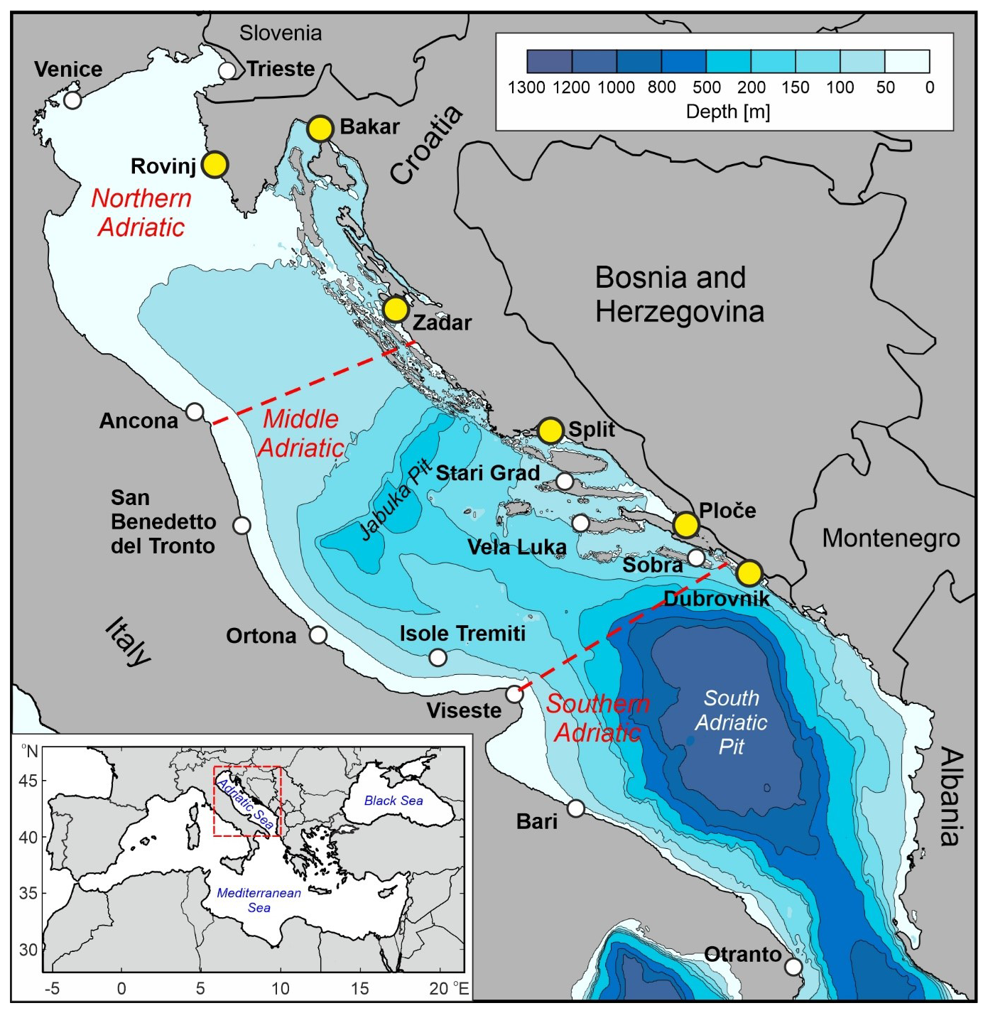
Figure 1 The bathymetry, locations, and names of tide gauge stations (circles) used in Ruić et al. (2023). Coloured yellow circles mark the tide gauges analysed in this paper. Publisher's remark: please note that the above figure contains disputed territories.

Numerous studies, particularly for the Mediterranean, have shown that the strongest atmospherically induced high-frequency sea level oscillations generally occur when distinct synoptic conditions prevail over the area. The pioneering studies go back to Ramis and Jansà (1983) for the Balearic Islands and to Hodžić (1988) for the Adriatic Sea. The characteristic conditions over the Mediterranean include a three-layer troposphere with a well-mixed, warm, and moist shallow surface layer extending to an altitude of ∼900 hPa. This layer is overlain by a temperature inversion, followed by a deeper layer, which is warm and dry in its lowest part but whose temperature decreases with a high rate and whose humidity and wind speed increase with altitude, possibly leading to conditionally or dynamically unstable mid- and upper-troposphere layers. On the horizontal scale, a low-pressure trough is often found to the west of the area where high-frequency sea level oscillations occur; warm air is advected from the southwest at altitudes higher than 900 hPa; and the front side of a deep upper-level trough, associated with strong mid- and upper-troposphere southwesterly winds, is located over the area. In the following decades, other authors documented similar favourable synoptic conditions for the Balearic Islands, the Adriatic Sea, and other Mediterranean locations (Jansà et al., 2007; Vilibić and Šepić, 2009; Šepić et al., 2009, 2015a, b). However, more recent research has shown that Mediterranean meteotsunamis also appear under different synoptic conditions, i.e. in situations dominated by deep extratropical cyclones that can, via the joint effect of a pressure drop and onshore winds, generate storm surges (Ferrarin et al., 2021; Šepić and Orlić, 2024). The extraction of synoptic patterns leading to strong high-frequency sea level oscillations has also been carried out for a couple of other worldwide locations using mostly subjective (visual) techniques (e.g. the Great Lakes coast – Bechle et al., 2016; the Baltic Sea – Pellikka et al., 2022). At these locations, several characteristic synoptic patterns have been recognised.

We aspire to classify and separate synoptic situations that lead to episodes of extreme high-frequency sea level oscillations from those leading to episodes of simultaneous extreme high- and low-frequency sea level oscillations, all for the Adriatic Sea. As already noted, our work builds on the paper by Ruić et al. (2023). Herein, we analyse the synoptic patterns that prevailed in the atmosphere during ∼300 episodes of high-frequency sea level extremes extracted by Ruić et al. (2023) from ∼16–18 years of 1 min sea level measurements at six Adriatic Sea tide gauges. We perform the classification by applying the k-medoids clustering method (Kaufmann and Rousseeuw, 1990) to the ERA5 reanalysis fields (Hersbach et al., 2020). The k-medoids algorithm, which groups objects to a predetermined number of clusters using a selected distance metric (in our case, the structural similarity index measure – SSIM), is explained in more detail in Sect. 2. The remainder of the paper is structured as follows: Sect. 2 outlines the materials and methods utilised; in Sect. 3, results are presented; and in Sect. 4, the discussion and conclusions are given.

2 Materials and methods

Ruić et al. (2023) analysed sea level series measured with a 1 min time step at 18 tide gauge stations located along the eastern and western coasts of the Adriatic Sea (Fig. 1). The length of the time series was 3–17.9 years. Prior to the analyses, the authors performed rigorous quality control of all sea level series, removing all non-physical spikes and outliers. Following this, the authors de-meaned and de-tided the series. The series were de-tided using the MATLAB T Tide package (Pawlowicz et al., 2002), with the tidal signal estimated for the seven constituents that are traditionally used for the Adriatic Sea tidal analyses, namely, K1, O1, P1, K2, S2, M2, and N2 (Kesslitz, 1919). Afterwards, the residual sea level series (the series without the tidal components and with subtracted mean values) were filtered with a 2 h Kaiser–Bessel window (Thomson and Emery, 2014), resulting in the formation of high-frequency (HF, T<2 h) and low-frequency (LF, T>2 h) series. The authors defined extremes on HF series using the peak-over-threshold method, defining all points in the HF time series that are above the 99.993 percentile threshold as extremes. These extremes were called “high-frequency” extremes (“HF extremes”, from this point on). Additionally, the authors noticed that there are situations in which HF extremes occur within ±24 h of extremes of residual series (termed “residual extremes” in Ruić et al., 2023), with the latter defined as periods when the residual sea level surpasses its 99.85 percentile. Herein, we term these “joint” events “compound extremes”. For both types of extremes (HF and compound), to ensure the independence of events, a condition was set that all points which surpass the percentile thresholds and appear within a 3 d window represent the same extreme episode. The tables of extreme episodes are available as datasets through Ruić et al. (2025a). As an example, in Fig. 2, we show one HF extreme and one compound extreme measured at the Bakar tide gauge (Fig. 1).

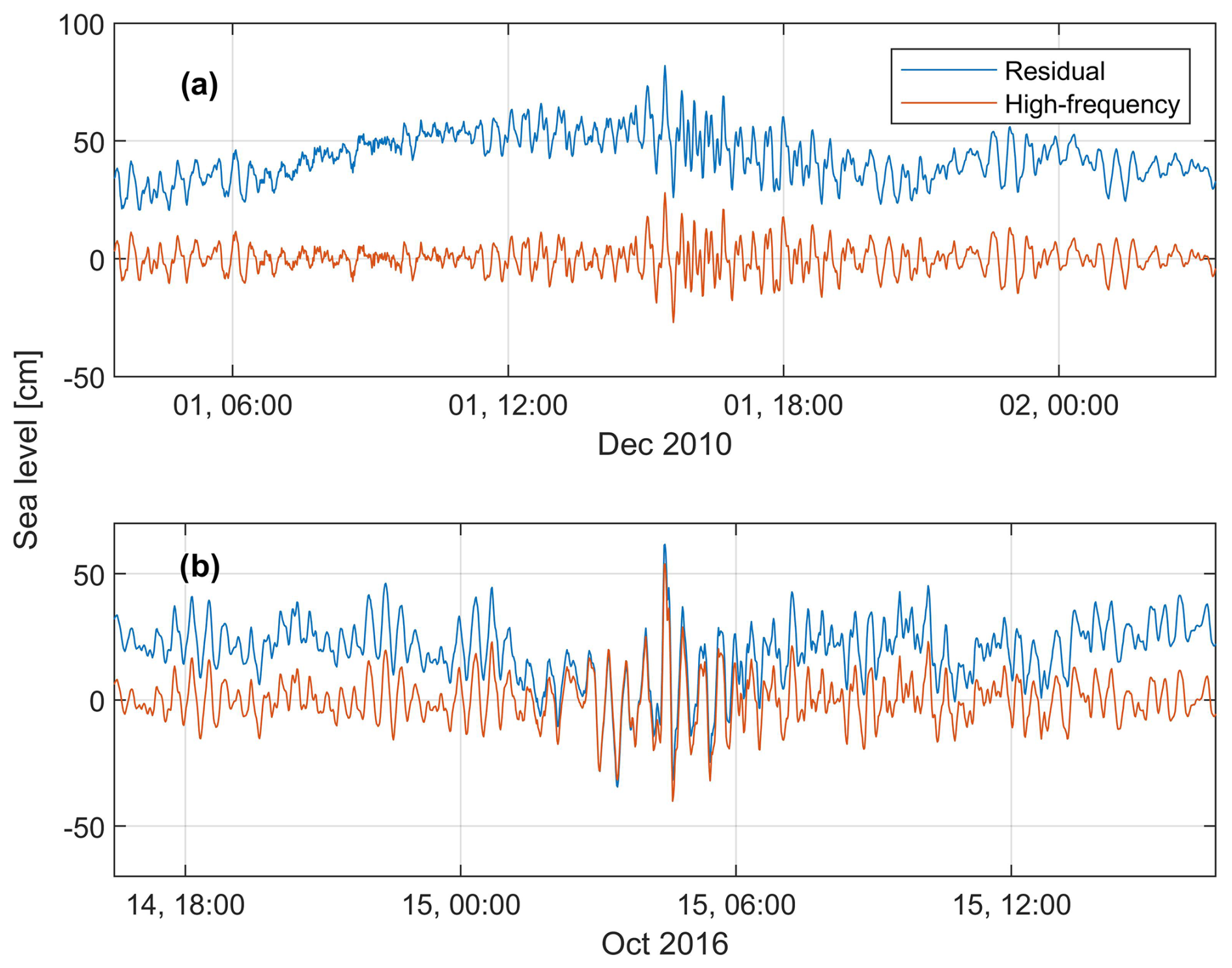
Figure 2 The (a) compound extreme that took place on 1 December 2010 and (b) HF extreme that took place on 15 October 2016, both at the Bakar tide gauge station.

In this paper, we classify synoptic situations that govern the appearance of HF and compound extremes at 6 tide gauge stations (out of 18 stations used by Ruić et al., 2023). These six stations (Rovinj, Bakar, Zadar, Split, Ploče, and Dubrovnik; Fig. 1) have the longest time series (16.4–17.9 years) and are evenly spread along the eastern coast of the Adriatic Sea. Unfortunately, time series measured at tide gauges located along the western Adriatic Sea have durations that are too short (from 6 to 10 years) to allow for the extraction of a sufficient number of extreme episodes to apply clustering methods. For the selected six stations, information on the HF and compound extremes (date, heights of residual, and the HF and LF component, for each event) was extracted from the paper or from data used by Ruić et al. (2023). Basic properties of HF and compound extremes at each station are listed in Table 1.

Table 1 The locations of tide gauges, the length of time series (in years), the percentile thresholds (in cm) for defining HF and compound extremes, and the number of both types of episodes (HF and compound) in the respective training and testing periods.

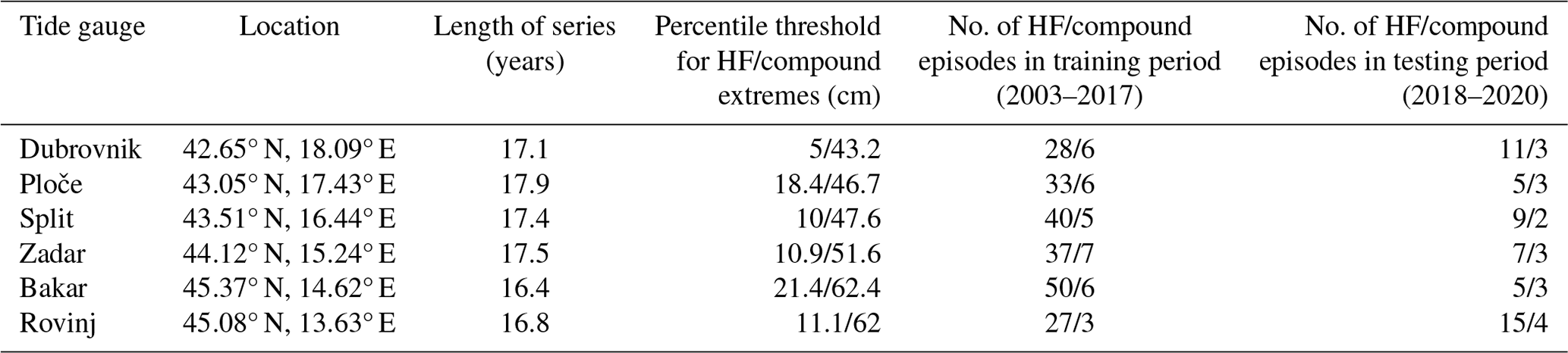
The data availability period was divided into two parts: the training and testing periods. The training period spanned from the start of the measurement (which was slightly different for each tide gauge – 1 January 2003 at the earliest and 19 June 2003 at the latest) until 31 December 2017, and the testing period spanned from 1 January 2018 until 31 December 2020.

Classification of synoptic conditions was performed by applying the k-medoids clustering method to the ERA5 reanalysis data (Hersbach et al., 2020; Copernicus Climate Change Service, 2017). After initial tests with a wider range of variables, we focused on the following: (i) mean sea level pressure (MSLP), (ii) temperature at 850 hPa, and (iii) geopotential height of 500 hPa. Herein, we note that favourable conditions for the generation of strong high-frequency sea level oscillations can usually be detected in spatial fields of these synoptic variables (e.g. Jansà et al., 2007; Vilibić and Šepić, 2009; Šepić et al., 2015b). The variables were downloaded for the area of the Adriatic Sea (approximate area shown in Fig. 1) for 12:00 UTC of the days of the training period on which HF or compound extremes occurred and for 12:00 UTC of each day of the testing period.

For each ERA5 variable, means and standard deviations of each month were calculated using the ERA5 data for the whole period (from 2003 until 2021). Synoptic data corresponding to each HF and compound extreme of the training set and to each day of the testing set were then normalised by subtracting the monthly mean and dividing the resulting series by the monthly standard deviation. Normalisation was done for each variable separately. All normalised variables (MSLP, temperature at 850 hPa, and geopotential height at 500 hPa) were concatenated to form a single vector (called a data point) for each day of the training period on which a HF or a compound extreme occurred as well as for each day of the testing period, and they can be accessed through Ruić et al. (2025a). Characteristic synoptic clusters were then obtained by applying the k-medoids algorithm on all vectors from the training period. Clustering is normally done by first selecting a number of clusters (n) and then iteratively evaluating the similarity of input vectors to each other. The process of evaluating is repeated until n input vectors (i.e. n vectors of synoptic variables related to one of the HF or compound extremes) most alike all of the other input vectors within a cluster are found. The vectors that are most alike all of the others inside a cluster (one per cluster) are called “medoids”, and these medoids basically represent normalised synoptic situations (MSLP, temperature at 850 hPa, and geopotential height of 500 hPa) on one of the training set days.

To determine medoids and to group all input vectors into clusters, we used the structural symmetry index measure (SSIM) as a distance metric. The SSIM was calculated as in Wang et al. (2004). If we take, for example, temperature and look at two different days on which a HF extreme occurred, setting x to be the vector of temperature for the first date and y to be the vector of temperature for the second date, the SSIM value (for temperature) is computed as follows:

$$\begin{array}{}\text{(1)}& \text{SSIM}(\mathit{x},\mathit{y})={\displaystyle \frac{(\mathrm{2}{\mathit{\mu }}_x{\mathit{\mu }}_y+c_{\mathrm{1}})(\mathrm{2}{\mathit{\sigma }}_{xy}+c_{\mathrm{2}})}{({\mathit{\mu }}_x^{\mathrm{2}}+{\mathit{\mu }}_y^{\mathrm{2}}+c_{\mathrm{1}})({\mathit{\sigma }}_x^{\mathrm{2}}+{\mathit{\sigma }}_y^{\mathrm{2}}+c_{\mathrm{2}})}},\end{array}$$

where μ_x and μ_y are the respective mean values of x and y (in our case, both equal to zero, as the series were normalised), σ_x and σ_y are their respective variances, and σ_xy is the covariance. Herein, c₁ and c₂ are the stabilisation coefficients that are necessary in situations in which the denominator (without c₁ and c₂) in Eq. (1) is close to zero. The stabilisation coefficients are computed as $c_{\mathrm{1},\mathrm{2}}=(K_{\mathrm{1},\mathrm{2}}L{)}^{\mathrm{2}}$, where L is the dynamic range of pixel values and K_1,2 are small (≪1) constants (see Wang et al., 2004, for further details on the computation of C_1,2, dynamical range, and K_1,2). The SSIM between two data points (vectors of synoptic variables) is calculated as the average of SSIM for temperature, mean sea level pressure, and geopotential height. This average SSIM is referred to as the SSIM value between two data points. These SSIM values, between all pairs of dates in the training set, are then passed as the distance matrix to the k-medoids algorithm. From that distance matrix, the method chooses the n medoids as the days with the maximal similarities to all other days.

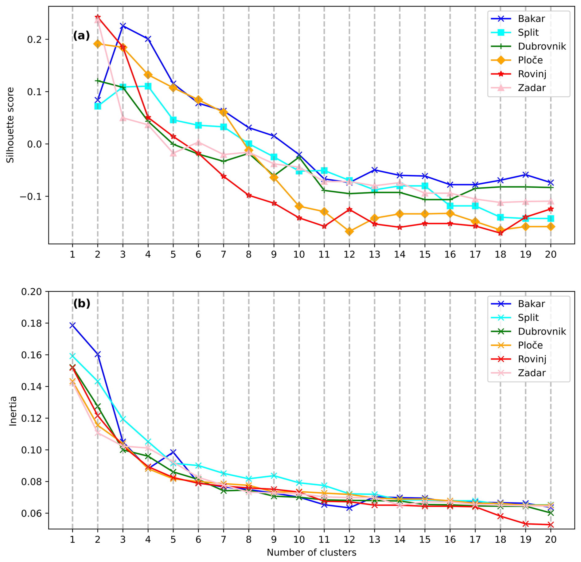
Figure 3 The (a) silhouette and (b) elbow methods for determining the optimal number of clusters. Each colour in the plots represent a different tide gauge station, as shown in the legend.

The silhouette and elbow methods were used to determine the optimal number of clusters for each station. The silhouette method is used to assess the quality of the preformed clustering depending on the number of clusters (Rousseeuw, 1987). For each data point in each cluster, the average SSIM value is calculated between that point and all other data points in that cluster (denoted as a). Then, for the same data point, the average SSIM value between that point and all other data points in the next-nearest cluster is calculated (denoted as b). The value of the silhouette score is then given by the following: $(\mathit{b}-\mathit{a})/max(\mathit{a},\mathit{b})$. Higher values indicate better matching of a data point to its assigned cluster and worse matching to the neighbouring cluster. A total silhouette score is obtained by estimating the mean value of all silhouette scores.

Another way of assessing the optimal number of clusters is the elbow method (Kodinariya and Makwana, 2013). The sum of squares of the SSIM values (called inertia here) is computed between each data point and the assigned medoid, within each cluster. Adding more clusters results in a decrease in inertia. If there are, for example, n characteristic situations, the inertia will become drastically smaller after these n situations are extracted. Once these situations are found, the increase in cluster number does not contribute significantly to a further reduction in the inertia value.

Figure 3 shows the results of applying the silhouette and elbow methods to our dataset. The silhouette method (Fig. 3a) shows that, for most stations, the highest scores are achieved when two to four clusters are used, with the optimal cluster number being the one with the highest silhouette score. For Rovinj, Zadar, Ploče, and Dubrovnik, the highest score is obtained when two clusters are used; for Bakar, the use of three clusters is the best choice; and for Split, the choice of three or four clusters gives approximately the same score. As for the elbow method, we are looking for a point at which the inertia value is low and at which the addition of new clusters does not decrease the inertia value significantly. For all of our stations, the elbow point is located somewhere between two and five clusters (Fig. 3b). Given the results of the silhouette and elbow methods, we have chosen to apply the k-medoids method by setting the number of clusters first to two and then to three; we then compare the results obtained with these two choices. The code used can be accessed at Ruić et al. (2025b).

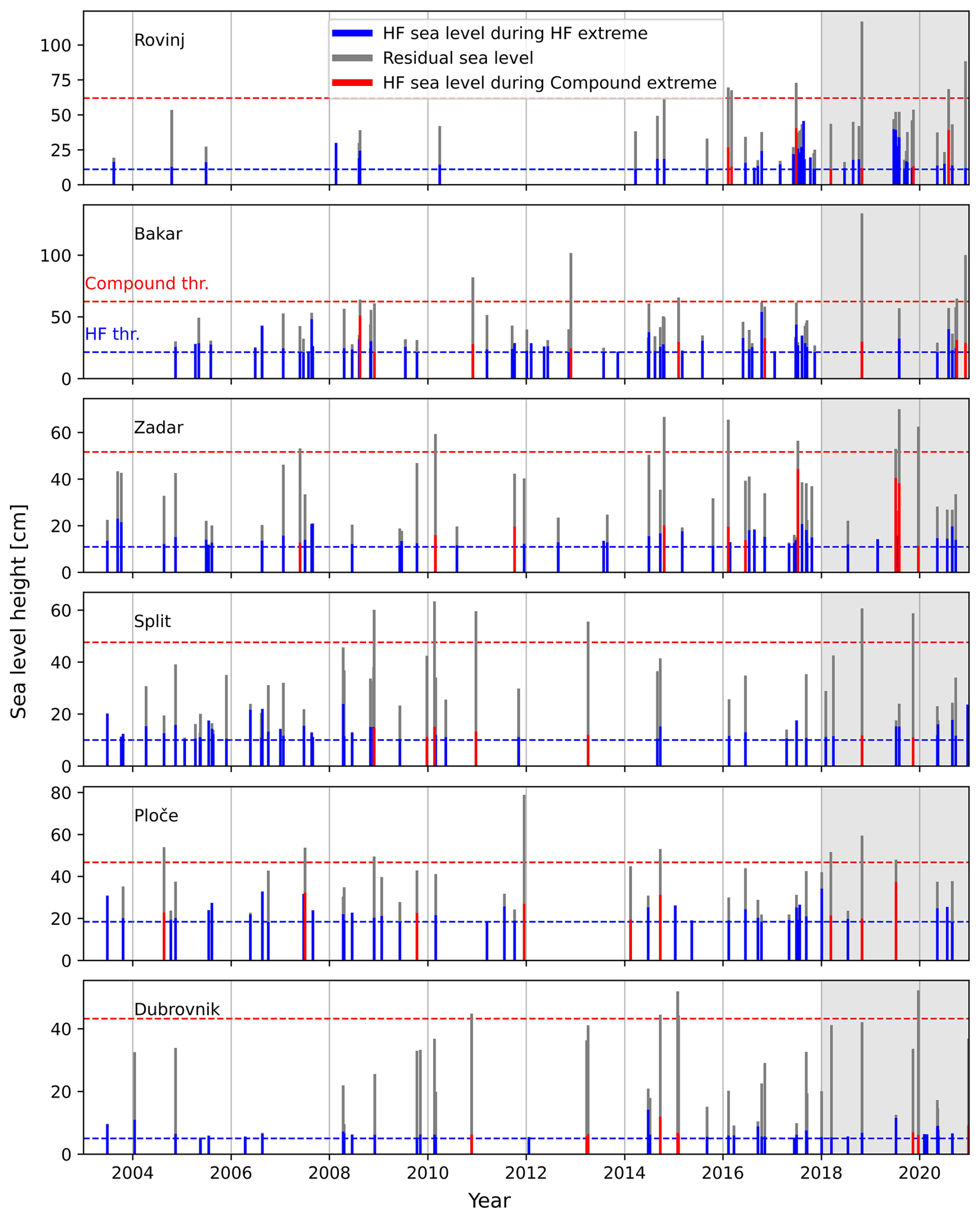
Figure 4 Temporal distribution of high-frequency sea level extremes at six tide gauge stations. Blue bars denote the HF sea level during HF extremes, red bars denote the HF sea level during compound extremes, and grey bars denote the residual sea levels for both types of extremes. The grey shaded area (2018–2021) marks the testing period, whereas the white area (2003–2018) marks the training period. The dashed red line marks the threshold of the residual sea level height for the definition of a compound extreme, while the dashed blue line marks the threshold of the HF sea level height for the definition of HF extremes.

3 Results

3.1 HF and compound extremes

As already stated, we differentiate two types of extreme episodes (previously extracted by Ruić et al., 2023): (1) HF extreme episodes, in which high-frequency sea level oscillations reached extreme values, and (2) compound extreme episodes, in which both high-frequency and residual series reached extreme values. The yearly distribution and heights of both types of extremes are shown in Fig. 4. At some tide gauges, e.g. Bakar and Zadar, events are evenly distributed through the years. At other stations, e.g. Rovinj, events are more abundant in one period (2016–2021) and are rare in other periods (2004–2014). In this specific case (Rovinj station), the change in the frequency of the appearance of HF episodes is probably due to the changes to the station's stilling well in 2016 and 2017: the connecting pipe first broke during a storm in 2016 and was then replaced with a new connecting pipe of a different shape and different attenuation properties (compared to the original pipe) in 2017. Both changes likely resulted in weaker damping of the high-frequency oscillations in the stilling well. Despite the changes, we retain events from Rovinj in our analysis because (i) more than half of the episodes detected during the 2016–2021 period in Rovinj are also recorded on other tide gauges and (ii) the results obtained for Rovinj station are in line with the results obtained for other tide gauge stations.

It can also be noticed that some events were captured at only one tide gauge station, whereas others were captured at multiple tide gauges; for instance, the compound extreme event on 29–30 October 2018 was recorded at the Rovinj, Bakar, Split, Ploče, and Dubrovnik stations.

The maximum sea level of HF and compound extremes is strongly dependent on the station, as is the contribution of the HF component to the total level. At Dubrovnik (the station with the weakest HF signal), the maximum residual sea level during HF extremes ranges from 5 to 52 cm, whereas at Bakar (the station with the strongest residual signal), the maximum residual sea level during HF extremes ranges from 4 to 134 cm (Fig. 4). The contribution of the HF component ranges from 5 to 14 cm at Dubrovnik and from 21.4 to 54 cm at Bakar. The residual sea level height during compound extremes ranges from 34 to 52 cm at Dubrovnik and from 58 to 134 cm at Bakar, with a contribution of the HF component from 6 to 12 cm at Dubrovnik and from 24 to 51 cm at Bakar. In Rovinj, Bakar, Zadar, and Ploče, the HF component occasionally contributed more than 50 % to compound extremes. On the other hand, at the Split and Dubrovnik stations, this contribution was lower than 30 % for all joint episodes.

The monthly distribution of two types of extreme episodes is shown in Fig. 5. At Rovinj and Zadar, there is a clear seasonal signal, with most of the HF extremes recorded from June to October. A similar distribution is present for Ploče and Bakar, although with comparable number of events in May as well. In Split, HF extremes peak from April to June and then again in August and November. At Dubrovnik, the number of HF extremes is even throughout the year, although an exceptionally low number of HF extremes are registered in August; this contrasts with most other stations, at which the highest number of events is registered in August. Regarding compound extremes, these events are clearly more abundant at the Bakar, Split, and Dubrovnik stations in the colder part of the year (October–December, with fewer events in January–April), in line with the known distribution of storm surges (Lionello et al., 2012; Ruić et al., 2023). At the Rovinj, Zadar, and Ploče stations, the seasonal distribution of compound extremes is not as pronounced. However, it should be noted that compound extremes at these three stations are occasionally dominantly due to the HF component; i.e. during certain episodes, the HF component is almost high enough to represent a compound extreme (even without an exceptionally high LF component) (Fig. 4). If we were to omit such episodes from compound extremes, the compound extremes would be most abundant in colder part of the year at Rovinj, Zadar, and Ploče as well (not shown).

Figure 5 Monthly distribution of the HF (orange bars) and compound (blue bars) extremes at six tide gauge stations, estimated for the entire period of measurements (2003–2021).

The different seasonal distributions of HF and compound extremes hint at the fact that there are at least two different synoptic situations that can produce strong HF oscillations, one associated with summertime conditions (presumably similar to “summer-type” or “good-weather” meteotsunami-favourable synoptic situations, as described in Rabinovich, 2020; Pellikka et al., 2022; and Lewis et al., 2023) and another associated with fall/winter conditions (presumably similar to “winter-type” or “bad-weather” meteotsunami synoptic situations, as also described in Rabinovich, 2020; Pellikka et al., 2022; and Lewis et al., 2023).

3.2 Characteristic synoptic patterns

De-normalised medoids, i.e. representative situations for each cluster, are presented in Figs. 6–8 (in panel (a) for a choice of two clusters and in panel (b) for a choice of three clusters in each figure). Medoids are shown for Bakar, Split, and Dubrovnik, which are selected as representative stations for the northern, middle, and southern Adriatic, respectively. Characteristic medoids for the other three stations (Rovinj, Zadar, and Ploče) are given in the Supplement (Figs. S1–S3). In all plots, the MSLP is shown in the first row, temperature at 850 hPa is shown in the second row, geopotential height of 500 hPa is shown in the third row, and box plots of the HF and LF sea level heights for episodes assigned to each cluster are shown in the fourth row.

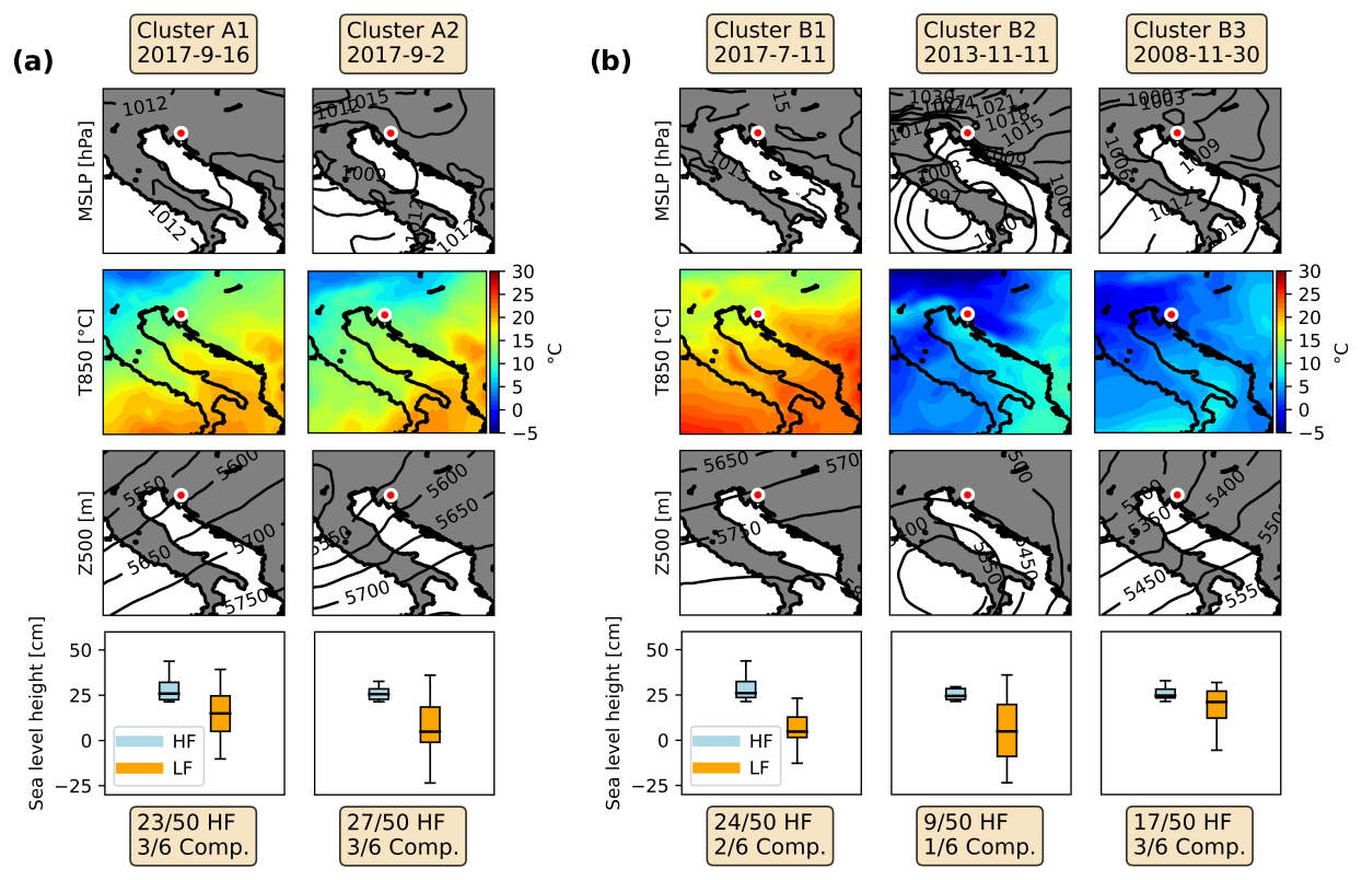
Figure 6 Medoids for a choice of (a) two and (b) three clusters for Bakar. The first three rows show the MSLP, temperature at 850 hPa (T850), and geopotential height of 500 hPa (Z500), respectively. The fourth row shows box plots of the HF (blue box) and LF (orange box) sea level heights during HF and compound extremes. The dates of medoids are given at the top of each column, and the location of the Bakar tide gauge is marked with a circle. Additionally, at the bottom of each column, the numbers of HF and compound extremes grouped in each cluster are given.

Figure 6 shows the results of the k-medoids clustering for Bakar. In accordance with the results shown in Fig. 3, the optimal number of clusters for the classification of the synoptic situations related to Bakar HF and compound extremes is three. The comparison with the medoids obtained for a choice of two clusters justifies this assessment. A choice of two clusters results in two similar medoids, whereas a choice of three clusters produces three different synoptic situations. Focusing firstly on a choice of two clusters, the medoid of the first cluster (Cluster A1) had a uniform (non-gradient) MSLP field over the Adriatic, while the Cluster-A2 medoid was characterised by weak MSLP gradients over the Adriatic Sea favouring a weak southeasterly sirocco wind. Gradients were due to a closed low located over the Gulf of Genoa. The two medoids differed less at the higher levels. The temperature fields, for both dates, revealed an inflow of warm air from the southwest in the low troposphere (850 hPa), while the parallel isohypses indicated that strong southwesterly mid-tropospheric winds (jet stream) were blowing at a height of 500 hPa. Both the jet stream and the inflow of warm air are known precursors to the generation of intense HF sea level oscillations in the Mediterranean (e.g. Šepić et al., 2015a). The similarity of both medoids is again confirmed by the box plots shown in the fourth row of Fig. 6a, where the distributions of the HF and LF sea level heights during extreme events associated with a specific cluster are given. These distributions are alike for both clusters, and a similar number of HF extremes and a same number of compound extremes are grouped into each of the two clusters.

For a choice of three clusters, the first medoid (Cluster B1) is like the two medoids obtained for a choice of two clusters. This refers to both the synoptic situation and the distribution of the HF and LF sea level heights during extremes. The Cluster-B2 medoid, on the other hand, represents a new synoptic situation. The surface situation, with an extratropical cyclone centred over the Tyrrhenian Sea, favoured northeasterly to northerly winds over the northern Adriatic (i.e. bora; Grisogono and Belušić, 2009); bora wind, which is characteristic of the Adriatic Sea, has, to the best of our knowledge, not previously been associated with intense HF sea level oscillations. At 850 hPa, a west–east temperature gradient was evident, while a closed low was located over the Tyrrhenian Sea at 500 hPa, resulting in ∼10 m s⁻¹ easterly winds over the northern Adriatic. The third medoid (Cluster B3) shows a situation in which the MSLP distribution favoured southeasterly sirocco wind and likely the development of a storm surge in the northern Adriatic. At 850 hPa, there was an inflow of warmer air from the southwest, while isohypses were densified and oriented in a way that implies the blowing of strong mid-tropospheric southwesterly winds at 500 hPa. Choosing three clusters (instead of two) resulted in clearer separation of episodes according to the maximum sea level height of the LF component: the median sea level heights and the number of compound extremes are largest for Cluster B3, indicating that this cluster represents situations favourable for the development of compound extremes (with high contributions from both the HF and LF components).

In summary, for the Bakar station, three distinct types of synoptic condition that favour intense HF oscillations (the strongest being meteotsunamis) can be distinguished: (i) the classic summer-type medoid (clusters A1, A2, and B1), similar to the Mediterranean meteotsunami-favourable patterns (Jansà et al., 2007; Šepić et al., 2015a); (ii) the bora-type medoid (Cluster B2); and (iii) the storm-surge medoid or winter-type pattern (Cluster B3).

Switching our attention to the middle Adriatic, Fig. 7 shows the medoids obtained for the Split station for a choice of two and three clusters. As shown in Fig. 3, the optimal number of clusters for Split is three; however, we already obtain separation of the HF and compound extremes with two clusters. Clusters A1 and A2 show two synoptic situations that differ at all studied levels. At the surface layer, both MSLP fields suggest the presence of a cyclonic pattern over the Mediterranean. However, isobars of the Cluster-A1 median were oriented in a way that led to southeasterly to easterly winds over the southern and middle Adriatic and to northeasterly winds over the northern Adriatic Sea, whereas isobars of the Cluster-A2 median were oriented in a way that led to southeasterly sirocco winds over the entire Adriatic Sea (with southeasterly winds being favourable with respect to an increase in the LF component). At 850 hPa, a northeast–southwest temperature gradient was evident over the Adriatic for Cluster A1, whereas a northwest–southeast gradient was evident for Cluster A2. The isohypses for both clusters revealed that strong mid-tropospheric winds were blowing in both situations. However, the isohypses (and related winds) were orientated differently, with west-northwesterly winds in Cluster A1 and southwesterly in Cluster A2. The box plot distributions of the HF and LF sea level heights (fourth row in Fig. 7a) show that the median of the LF sea level heights was larger in Cluster A2 and that all compound extremes were grouped in Cluster A2.

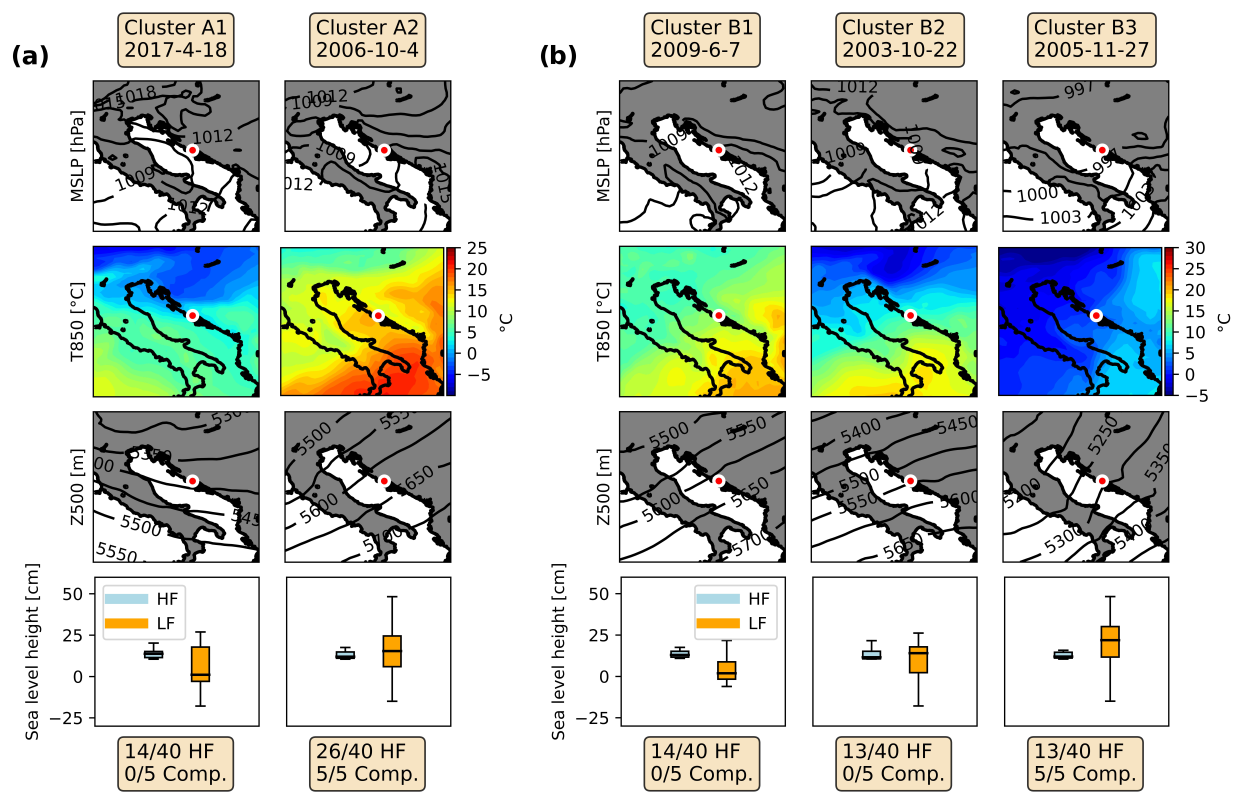
Figure 7 Medoids for the choice of (a) two and (b) three clusters for Split. The first three rows show the MSLP, temperature at 850 hPa (T850), and geopotential height of 500 hPa (Z500), respectively. The fourth row shows box plots of the HF (blue box) and LF (orange box) heights during HF extremes assigned to each medoid. The dates of medoids are given at the top of each column, and the location of the Split tide gauge is marked with a circle. Additionally, at the bottom of each column, the numbers of HF and compound extremes labelled in each cluster are given.

Looking at the three-cluster choice (Fig. 7b), the first two medoids (clusters B1 and B2) appear to be like the previously described summer-type medoid extracted for Bakar (Cluster B1; Fig. 6b). However, the MSLP isobars of the Cluster-B2 medoid reveal presence of southeasterly winds over the southern and middle Adriatic, leading to higher LF values at the Split tide gauge. The medoid of Cluster B3 resembles the winter-type medoid extracted for Bakar (Cluster B3; Fig. 6b). Thus, unsurprisingly, out of all of the HF episodes, those with the highest LF values were grouped in Cluster B3, as were all compound extremes.

In summary, two characteristic synoptic situations and one transitional synoptic situation for the generation of strong HF oscillations in Split were extracted: one which is related to the summer-type (meteotsunami) pattern (Cluster B1); one which is related to the winter-type (storm-surge) pattern (Cluster B3); and one “transitional” pattern, which has characteristics of both the summer-type (temperature field at 850 hPa) and winter-type (MSLP distribution) patterns (Cluster B2).

For the southern Adriatic, medoids for a choice of two or three clusters are shown for the Dubrovnik station (Fig. 8). Focusing on panel (a), we can see that the medoids for clusters A1 and A2 both have uniform (non-gradient) MSLP fields over the Adriatic Sea. At 850 hPa, the medoid of Cluster A1 shows the advection of warm air from the southwest, whereas a north–south temperature gradient was present over the area for the medoid of Cluster A2. Isohypses at 500 hPa had different orientations for clusters A1 and A2 (third row in Fig. 8a), with southwesterly flow favoured in Cluster A1 and westerly to west-northwesterly flow favoured in Cluster A2. The two medoids are clearly separated by the contribution of the LF component to extremes. The LF component was significantly higher for events belonging to Cluster A2. Additionally, five out of six compound extremes were grouped in Cluster A2.

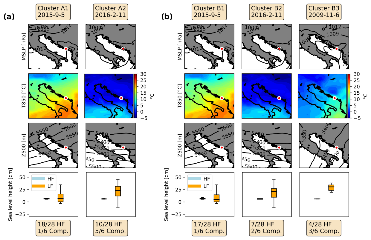
Figure 8 Medoids for the choice of (a) two and (b) three clusters for Dubrovnik. The first three rows show the MSLP, temperature at 850 hPa (T850), and geopotential height of 500 hPa (Z500), respectively. The fourth row shows box plots of the HF (blue box) and LF (orange box) heights during HF extremes assigned to each medoid. The dates of medoids are given at the top of each column, and the location of the Dubrovnik tide gauge is marked with a circle. Additionally, at the bottom of each column, the numbers of HF and compound extremes labelled in each cluster are given.

Looking at Fig. 8b, in which the medoids for a choice of three clusters are shown, we can see that the first two medoids (clusters B1 and B2) are the same as the medoids for a choice of two clusters. This indicates that these two medoids represent the training set of events so well that even an increase in cluster number does not lead to their change. The third medoid (Cluster B3) had a low-pressure centre located over the middle Adriatic, resulting in alongshore and onshore winds at the Dubrovnik coast. At 850 hPa, there was again the advection of warm air from the southwest, while isohypses were oriented in a southwest–northeast direction at 500 hPa, with southwesterly winds with speeds of ∼30 m s⁻¹ blowing over the southern Adriatic (not shown). The box plot distribution of the HF and LF sea level heights during the extremes reveals that Cluster B3 contains episodes with the highest LF signal. This cluster has the least HF extremes (4 out of 28) attributed to it but the most compound extremes (3 out of 6).

In summary, there are three characteristic situations for occurrence of strong HF oscillations in Dubrovnik: (i) a classic summer-type pattern (clusters A1 and B1), (ii) a transitional-type pattern (Cluster B2), and (iii) a winter-type pattern (clusters A2 and B3).

Characteristic medoids for the other three stations, Rovinj, Zadar, and Ploče, are given in the Supplement. At these three stations, the obtained medoid patterns can be classified as follows: (i) a summer-type pattern (uniform MSLP, the advection of warm air from the southwest in the lower troposphere and strong southwesterly winds in the mid-troposphere, and a lower LF component), (ii) a winter-type pattern (MSLP gradients favouring sirocco winds, which can induce storm surges; colder lower troposphere and strong southwesterly winds in the mid-troposphere; and a higher LF component and more compound extremes), (iii) a transitional-type pattern (at Zadar and Ploče), and (iv) a bora-type pattern (in Rovinj).

Figure 9 shows, separately for a choice of two or three clusters, the monthly distributions of the number of HF and compound extremes within different clusters. Starting with a choice of two clusters, at the Rovinj, Zadar, Ploče, and Dubrovnik stations, the medoids associated with Cluster A1 are more common in the summer months (June–August), whereas the medoids associated with Cluster A2 are more common in the colder part of the year. This agrees with the summer-type vs. winter-type classification. At Bakar and Split, clusters A1 and A2 appear almost evenly throughout the year, confirming that a choice of two clusters did not result in the optimal extraction of synoptic situations at these two stations.

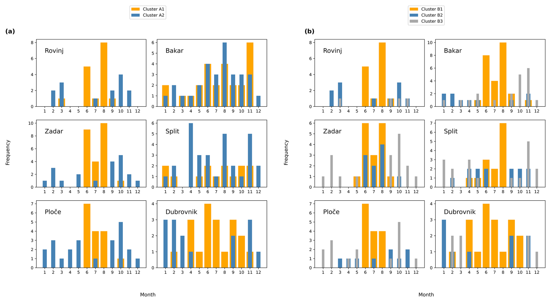
Figure 9 Monthly distribution of cluster labels for each event in the training part of the dataset.

Changing the cluster number from two to three (Fig. 9b), we now notice that summer-type (Cluster B1) and winter-type (Cluster B3) clusters are separated at all stations. The second cluster (Cluster B2), on the other hand, (i) represents a refinement of either the summer-type cluster (in Zadar) or (ii) the winter-type cluster (Ploče and Dubrovnik), (iii) introduces a new (also winterish, peaking in January and February) bora synoptic situation (Rovinj and Bakar; Figs. 6b and S1), or (iv) is now associated with spring and autumn events (Split).

Observed seasonal distributions are in line with what is known regarding the climatology of weather patterns over Croatia: calm weather conditions are predominant in summer, extratropical cyclones leading to storm surges peak in autumn but also happen in winter (December–February) (Lionello et al., 2012), and bora conditions peak in winter (i.e. December–February) but can also happen in autumn (Poje, 1992).

3.3 Testing period

After classifying the HF and compound extremes from the training dataset into their representative clusters, we tested the classification by feeding the k-medoids algorithm with input vectors (data points) corresponding to selected synoptic variables of 1096 d of the testing period (days from 1 January 2018 until 31 December 2020). For each day of the testing period, for each station, and for a choice of two or three clusters, daily synoptic situations (concatenated to vectors consisting of normalised fields of the MSLP, temperature at 850 hPa, and geopotential height of 500 hPa for 12:00 UTC of each day) were compared to characteristic medoids (as extracted from the training period; Figs. 6–8 and S1–S3). Each day of the testing period was assigned to one of the clusters, depending on the SSIM value, i.e. the difference in the synoptic situation of that day and the synoptic situation of representative medoids, with the primary aim of checking whether SSIM values were higher on days in which HF or compound extremes were registered (higher SSIM values suggest higher similarity between fields) than on random days.

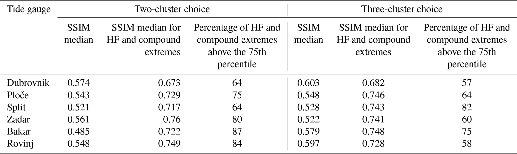
Box plots of the resulting SSIM distributions for each day, cluster, and station of the testing period are shown in Fig. 10. In all plots, black dots represent SSIMs for days of the testing period on which an extreme HF or compound event occurred (based on data used by Ruić et al., 2023). As can be seen in Fig. 10, most SSIM values were above the 75th percentile value (upper edge of boxes) during HF and compound extremes of the testing period, and all (but four) values were above the median value of their respective medoid. At some stations, a choice of two clusters (vs. three clusters) resulted in a better classification of events in the testing period. This holds for Zadar and Rovinj, where both the SSIM median of HF and compound extremes and the percentage of events with an SSIM above the 75th percentile decreased when we increased the number of clusters from two to three (Table 2). At other stations (Dubrovnik, Ploče, and Bakar), the SSIM median increased (implying better classification), but the percentage of events with an SSIM above the respective 75th percentile decreased (implying worse classification) when we increased the number of clusters. Finally, increasing the number of clusters is clearly beneficial for the Split station, where both the SSIM median and the percentage of events with an SSIM above the corresponding 75th percentile increased when we increased the number of clusters.

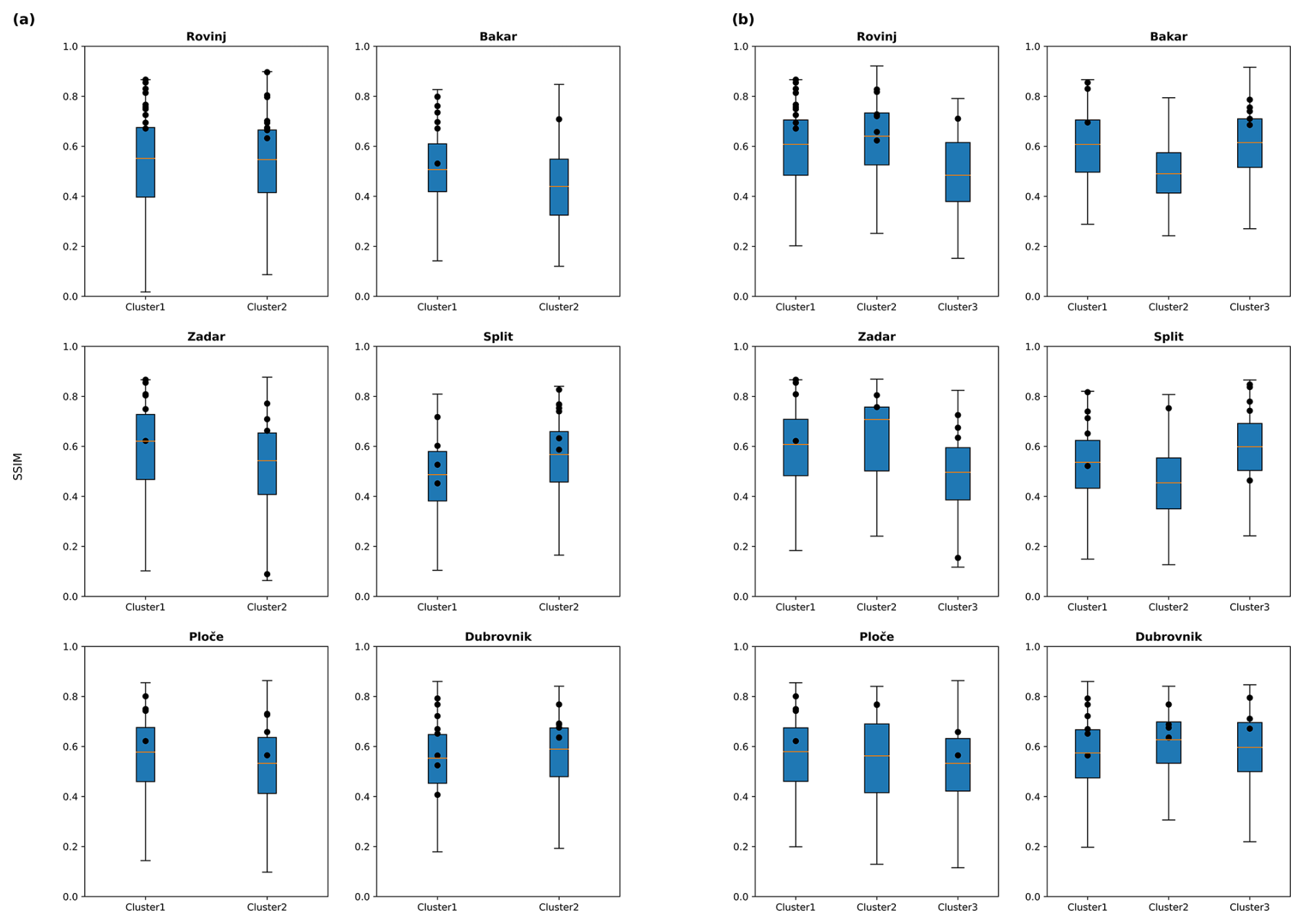
Figure 10 Box plots of the SSIM values for each day of the testing period, depending on the assigned cluster. Plots are given for each station for a choice of (a) two and (b) three clusters. Black dots indicate the dates of the testing period that contain episodes of extreme HF oscillations (both HF and compound extremes). With respect to the box plots, orange lines denote median values; the upper and lower edges of the blue boxes denote the 75th and 25th percentile values, respectively; and whiskers denote the minimum and maximum values.

Table 2 Values of the SSIM median for all days of the testing period (regardless of the cluster to which these days were assigned), the SSIM median of all episodes of HF and compound extremes, and the percentage of all HF and compound extremes above the corresponding 75th percentile, for a choice of two (left) and three (right) clusters.

At Zadar there is one episode that could be considered an “outlier” (Fig. 10). Regardless of the number of clusters, this episode “scores” very low. The related synoptic situation was characterised by exceptionally strong sirocco winds blowing over Zadar, a uniform temperature field at 850 hPa, and a closed low over the Ionian Sea that was detectable at 500 hPa, differing significantly from extracted Zadar medoids (Fig. S2).

It is important to note here that the number of events per station in the testing periods ranges from 5 to 15 for HF extremes and from 2 to 4 for compound extremes (Table 1) and that longer period measurements would be beneficial for obtaining more robust statistics.

3.4 Method selection

There are many methods available for clustering data, such as k-means, self-organising map (SOM), and k-medoids techniques. We have chosen k-medoids with the SSIM as the distance measure. In this section, we clarify our reasoning with respect to the choice made.

To find characteristic synoptic fields that are related to certain process (in this case, intense HF sea level oscillations), both subjective and objective approaches can be implemented. Subjective approaches require an observer who manually classifies the synoptic situations based on previous experience and gained knowledge (which can be solely manual, as in Muller, 1977, or manual after some programming filter, as in Sheridan, 2002). This approach is useful for a qualitative analysis and has already been applied to the problem at hand by researchers such as Ramis and Jansà (1983), Šepić et al. (2015a), Bechle et al. (2016), and Pellikka et al. (2022). However, this approach becomes more difficult and time-consuming as the dataset gets larger. A possible solution to this is to use mathematical methods for classification (i.e. an objective approach) that diminish the mentioned issues. The most popular methods for classification are k-means clustering, SOMs, and the herein-presented k-medoids method, all of which have been used to classify various problems in atmospheric physics, such as North Atlantic climate variability (Reusch et al., 2007), synoptic- and local-scale wind patterns in Tyrrhenian coastal area (Di Bernardino et al., 2022), and the reconstruction of ocean surface temperature and salinity (Elken et al., 2019). Additionally, empirical orthogonal function (EOF) analysis and principal component analysis (PCA) have been used by various authors, both independently and as dimensionality reduction techniques that precede one of the cluster methods (Philippopoulos et al., 2014; Gao et al., 2019).

The k-means and SOM classification methods are known to generate good results, but they have some underlying problems that need to be kept in mind. Firstly, the centres of clusters are mean values of each cluster element, potentially clouding the physical processes that are driving the events in each cluster and resulting in a loss (due to averaging) of some valuable information about the synoptic situation. The commonly used distance metric in k-means and SOM is the Euclidian distance. This distance metric takes point-to-point distances and, thus, occasionally leads to misleading results; for example, a pressure low separated by only a few points in two events will sometimes result in a large Euclidian distance, although the two situations are physically very similar (we are more interested in the gradients associated with the low than in the exact value of the low). Moreover, regarding this particular problem, a low number of events in the training set (from 30 to 56 – sum of HF and compound; Table 1) can represent a problem for k-means and SOM algorithms. These issues can be somewhat overcome by using different normalisation methods on the input data that help to improve the results (Milligan and Cooper, 1988). An extra problem arises when the input data are chosen to be a compound of different variables. This enlarges the dimensionality of input data and requires a lot more events for SOM and k-means to be trained effectively (Wang et al., 2019).

The issue of large dimensionality and a small number of training events can be somewhat resolved by using the k-medoids algorithm, which chooses specific events (medoids) rather than average values, to represent clusters. The k-medoids method allows for a better representation of the physical process that are in the background of each event and that can be better understood by examining the characteristic medoid (Winderlich et al., 2024). The problem of the distance metric is amended by using the structural similarity index measure (SSIM). This measure treats input fields as images (Hoffmann et al., 2021) and ensures that similar synoptic situations get grouped accordingly.

To test which of the three above-mentioned methods (k-means, SOM, or k-medoids) is optimal for our problem, we used all three separately to find clusters of the training set and then to label (associate them with a cluster) all days in the testing period (comparison of the three methods is shown in Fig. 11 for Bakar). For the k-means and SOM methods, the Euclidian distance was used as a distance metric, whereas the SSIM method was used for k-medoids. In Fig. 12, black dots represent days during the testing period on which an extreme (HF or compound) event occurred. The y axis shows the normalised distances; i.e. the smaller the value, the closer (more similar) the day to its cluster centre (for SOM and k-means) or to its medoid (for k-medoids). We notice that almost all events (black dots) happen when the normalised distance is small for the k-medoids method, in comparison to the other two methods, regardless of the number of clusters. For the k-means method, regardless of the choice of two or three clusters, the events occur with no clear connection to the normalised distance. The same thing can be said for the SOM method: for one cluster, events happened when the normalised distance was extremely large and when it was extremely small. Conclusively, we can say that, out of the three tested methods, k-medoids works the best in our situation.

4 Discussion

Traditionally, HF sea level extremes in the Adriatic (and similarly in the Mediterranean) have been associated with a single synoptic pattern characterised by a non-gradient (uniform) pressure field over the Adriatic, an inflow of warm air from the southwest in the lower troposphere, and the presence of the front side of a deep trough (with strong southwesterly winds over the Adriatic) in the middle and high troposphere (Jansà et al., 2007; Vilibić and Šepić, 2009; Šepić et al., 2009, 2015a, b). The work presented here led to the detection of a similar pattern (Cluster B1; Figs. 6–8 and S1–S3) that was mostly associated with HF extremes that occurred from June to September (Fig. 9); we labelled this synoptic situation the “summer-type” pattern. However, we detected at least one or, at some stations, two additional synoptic patterns that were clearly different from the summer-type pattern and that were present over the Adriatic during other HF and compound extremes. The second distinct pattern (Cluster B3; Figs. 6–8 and S1–S3) was characterised by pronounced MSLP gradients over the Adriatic, leading to strong southeasterly winds at the surface, an inflow of warm air in the lower troposphere (with the atmosphere generally cooler than during summer events), and (again) the presence of the front side of a deep trough in the middle and upper troposphere. This pattern was mostly assigned to HF and compound extremes that occurred during colder half of the year (Fig. 9); thus, we labelled it the “winter-type” pattern. Summer- and winter-type patterns mostly differed at the surface, whereas they were more similar at higher altitudes. The differences in surface weather were reflected in differences in the LF component of sea level. The summer-type pattern, for which there were no strong MSLP gradients or winds, was associated with average or slightly higher than average background (LF) sea level heights (fourth row in Figs. 6–8 and S1–S3). On the other hand, the winter-type pattern, for which the MSLP was lower than average with pronounced gradients and for which we noted strong southeasterly winds, was associated with above average background (LF) sea levels (fourth row in Figs. 6–8 and S1–S3). The distinction also resulted in the summer-type pattern being more typical of HF extremes and the winter-type pattern being more typical of compound extremes. The herein-extracted winter-type pattern is clearly similar to a storm-surge-favourable pattern, as recognised for the Adriatic Sea by researchers such as Lionello et al. (2012). Finally, we also extracted an additional synoptic pattern (Cluster B2; Figs. 6–8 and S1–S3). At most of the stations, this is a transitional-type pattern and presents a refinement of either the summer- or winter-type pattern. However, at the Bakar and Rovinj stations, the additional pattern (Cluster B2; Figs. 6 and S1) described a new situation with pronounced MSLP gradients and moderate to strong northeasterly winds (i.e. bora, Grisogono and Belušić, 2009) blowing over the area, suggesting that additional, previously unrecognised, types of weather systems may lead to strong HF sea level oscillations along some coastal stretches.

The extraction of two additional synoptic patterns related to HF sea level oscillations represents a novelty of our work, as only the summer-type pattern has been recognised as characteristic for the occurrence of HF sea level oscillations in the Adriatic and Mediterranean Sea to date (aside from a few recent exceptions, such as Pérez-Gómez et al., 2021, and Ferrarin et al., 2021). We particularly stress the recognition of the winter-type pattern that is often found over the area during compound extremes, i.e. sea level extremes in which both the HF and LF components (the latter usually as a storm surge) contribute jointly to the overall height of the extreme. The importance of evaluating the HF sea level oscillations when assessing the total flood heights during a storm surge has only recently been acknowledged (Pérez-Gómez et al., 2021; Heidarzadeh and Rabinovich, 2021; Medvedev et al., 2022; Rabinovich et al., 2023), and our work represents an important contribution to such an assessment by confirming that HF sea level extremes can occur during synoptic situations that favour the development of storm surges. Furthermore, local bathymetry, the shape of the harbour/bay, its Q factor, and the orientation of the harbour/bay entrance all play an important role in determining the final height of HF sea level oscillations (Rabinovich, 2009). Ruić et al. (2023) classified the Adriatic Sea tide gauge stations in three groups depending on the contribution of HF oscillations to extremes: Group 1 contained stations at which HF oscillations were least important, Group 2 contained stations at which HF oscillations were moderately important, and Group 3 contained stations at which HF oscillations were most important. Ruić et al. (2023) note that Group-1 stations are mostly located along the open coast, Group-2 stations are located within wide bays and channels or within bays and channels that are protected from incoming long ocean waves by islands and peninsulas, and Group-3 stations are located in bays with large Q factors or within narrow channels. Three of the stations considered in this paper fall into Group 1 (Rovinj, Split, and Dubrovnik), while three fall into Group 2 (Bakar, Zadar and Ploče). Unfortunately, no stations from Group 3 had a sufficiently long data series for the analysis carried out herein.

Although the primary aim of our work was to extract and classify synoptic patterns characteristic of HF and compound extremes in the Adriatic Sea, our results raise an important question regarding the applicability of the k-medoids algorithm to forecasting HF and compound extremes. The evaluation of synoptic fields with the aim of forecasting “rissagas” (local name for meteotsunamis) has been done for the Balearic Islands since 1985 (Jansà and Ramis, 2021) and has been based on the premise that the greater the similarity (visually assessed) of the forecasted synoptic fields to the rissaga-favourable synoptic situation, the higher the probability of a strong meteotsunami. Šepić et al. (2016) suggested a method for quantifying the Balearic rissaga forecast by proposing a meteotsunami synoptic index that associates the average height of short-period sea level oscillations in Ciutadella (Balearic Islands) to a linear combination of selected synoptic variables (e.g. wind speed and direction in the low and mid-troposphere and gradients of MSLP and temperature). Both the probabilistic forecast (Jansà and Ramis, 2021) and meteotsunami index (Šepić et al., 2016) have proven successful with respect to predicting “no-rissaga/rissaga” conditions (if there is no favourable synoptic pattern, there will be no rissaga; if there is a pattern, there could be a rissaga), but both have been less successful with respect to predicting rissaga strength. Additionally, both are strictly related to one characteristic synoptic situation.

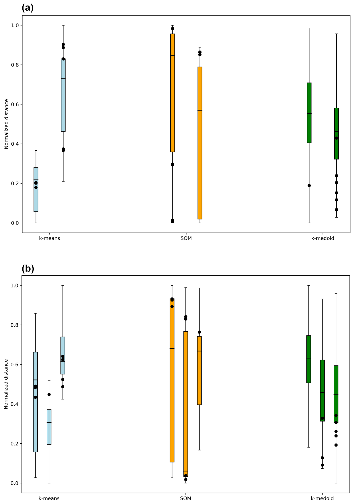
Figure 11 Box plots of normalised distances between each day of the testing period and the assigned cluster for a choice of (a) two and (b) three clusters. Black dots represent the days in the testing period on which HF or compound extreme events occurred. The analysis was carried out for three methods, k-means, SOMs, and k-medoids, for the Bakar tide gauge.

Unfortunately, when it comes to forecasts, our k-medoids classification algorithm suffers from the same problems as the two methods applied to the Balearic Islands. Ideally, we would say that HF sea level oscillations will be greatly amplified when the synoptic situation over an area is such that it strongly resembles one of the herein-extracted synoptic patterns. However, as Figs. 10 and 11 reveal, we are still a long way from reaching this conclusion. At most stations, most of the extremes during the test periods did occur at times when the synoptic conditions were similar to the extracted patterns (SSIM above the 75th percentile). However, there are obviously many other days on which the synoptic conditions were similar to the extracted patterns but on which HF or compound extremes were not registered. It seems that our analysis once again confirms the conclusions of Šepić et al. (2016): the presence of favourable synoptic conditions is a necessary but insufficient condition for the strong amplification of HF sea level oscillations, as synoptic maps “miss” the mesoscale atmospheric disturbances that generate intense HF sea level oscillations.

Nevertheless, the k-medoids classification method could be used to complement other methods for forecasting extreme HF sea level oscillations. For example, in situations where one of the specific patterns is observed/predicted (i.e. in situations where there is a high SSIM score between the predicted synoptic field and one of our clusters), additional attention could be paid to higher-resolution atmospheric and ocean models (as described, for example, in Denamiel et al., 2019, and Mourre et al., 2021), neural network methods (e.g. Vich and Romero, 2021), and real-time air pressure and sea level measurements (e.g. Marcos et al., 2009). Here, we stress that it is precisely the combination of different elements (synoptic assessment, high-resolution modelling, and real-time measurements) that has been recognised as a necessity for the development of an efficient system for monitoring and forecasting meteorological tsunamis (as the most destructive type of atmospherically triggered HF sea level oscillations) (Vilibić et al., 2016).

5 Conclusion

In summary, the main conclusions of our analysis are as follows:

1. Two characteristic synoptic patterns related to HF and compound extremes, a summer-type and a winter-type pattern, were identified.

2. The summer-type synoptic pattern is characterised by a relatively uniform MSLP field over the Adriatic Sea, an inflow of warm air from the southwest in the lower troposphere, and the presence of the front side of a deep trough (with strong southwesterly winds over the Adriatic) in the middle and high troposphere.

3. The winter-type synoptic pattern is characterised by pronounced MSLP gradients over the Adriatic Sea, leading to strong southeasterly winds at the surface, an inflow of warm air in the lower troposphere (with the atmosphere generally cooler than during summer events), and (again) the presence of the front side of a deep trough in the middle and upper troposphere.

4. The third extracted pattern either represents (i) a refinement of the summer- or winter-type pattern or (ii) a completely new synoptic situation.

5. At Bakar and Rovinj, the third pattern is characterised by pronounced MSLP gradients, leading to bora wind.

6. The k-medoids method is a valuable tool for the classification of synoptic patterns, especially when paired with the SSIM as the distance metric.

7. Favourable synoptic conditions represent necessary but insufficient conditions for the appearance of extreme HF events.

8. The prediction of intense HF extremes is not feasible with this framework (using only the k-medoids method), but the general probability of the occurrence of a HF extreme can be given according to the general similarity of a given synoptic situation to the characteristic medoids. Combining the k-medoids classification with high-resolution atmospheric/ocean models, neural network approaches, and real-time observations could improve the accuracy of forecasts of HF sea level oscillations.

9. Finally, increasing the sampling rate of the tide gauges could be useful, as it would allow for the assessment of the contribution of sea level oscillations with an even shorter period (e.g. wind waves, swells, and infragravity waves) to total sea level extremes.